Article

Impact of Pseudo-Stochastic Pulse and Phase Center Variation on Precision Orbit Determination of Haiyang-2A from Experimental HY2 Receiver GPS Data

1
College of Geodesy and Geomatics, Shandong University of Science and Technology, Qingdao 266590, China
2
National Satellite Ocean Application Service, Ministry of Natural Resources, Beijing 100081, China
3
School of Land Science and Technology, China University of Geosciences (Beijing), Beijing 100083, China
4
Land Satellite Remote Sensing Application Center, Ministry of Natural Resources, Beijing 100048, China
*
Author to whom correspondence should be addressed.
Remote Sens. 2024, 16(8), 1336; https://doi.org/10.3390/rs16081336
Submission received: 4 March 2024 / Revised: 8 April 2024 / Accepted: 9 April 2024 / Published: 10 April 2024
(This article belongs to the Special Issue Space-Geodetic Techniques II)

Abstract

:
Haiyang-2A (HY-2A) is the first marine dynamic environment satellite established by China, which has made significant contributions to the marine scientific research field. It carries the satellite-based GPS receiver named HY2, which was independently developed by China. It is an experimental satellite-borne GPS receiver for low earth orbit satellites, and during its operational period in orbit, the satellite-borne GPS data are not made accessible to the public. Therefore, this paper assesses the quality of HY-2A satellite-borne GPS data based on indicators such as satellite visibility, multipath effect, and ionospheric delay. The results indicate that the data acquired by the HY2 receiver are of high quality. The precise orbit determination (POD) uses the reduced-dynamic (RD) method. The adjustment effects of the pseudo-stochastic pulse time interval and a priori sigma on POD are analyzed, and the antenna phase center variation (PCV) is estimated using the direct method and residual method. Furthermore, this paper investigates the impact of PCV models with different resolutions (10° × 10° and 5° × 5°) on satellite orbit determination. To evaluate the orbit precision, three methods are used for validation, including carrier phase residual analysis, external precise science orbit (PSO) validation, and SLR three-dimensional (3D) validation, respectively. The results indicate that the highest orbit precision is achieved when the pseudo-stochastic pulse time interval is configured to 15 min, with the a priori sigma of 1 × 10⁻⁸ m/s2. The orbit carrier phase residuals reach the millimeter level. The 10° × 10°PCV model was estimated using the direct method and residual method, respectively; the root mean square of the external orbit validation for both methods show a millimeter-level improvement. The results obtained from the direct method and residual method are comparable. The resolution is increased from 10° to 5°, and the improvement in orbital precision is relatively small. The results obtained from the SLR 3D validation are consistent with those from the external PSO validation. The experimental results contribute valuable information for the POD of the HY2 series satellites.

1. Introduction

The Haiyang-2A (HY-2A) is the first marine dynamic environment monitoring satellite established by China, and it was successfully launched at the Taiyuan Launch Center in Shanxi Province on 16 August 2011. Its launch propelled China’s marine dynamic monitoring into the forefront of international advancement [1]. The HY-2A satellite has a mass of 1575 kg and operates in a sun-synchronous orbit with an inclination angle of 99.34°, which includes two orbit stages. In the first stage, the HY-2A orbits at an altitude of 971 km and has an orbit revisit period of 14 days. In the second stage, the HY-2A satellite’s orbit altitude is increased to 973 km, and the revisit period is adjusted to 168 days. [2]. The HY-2A satellite ended its observation mission in December 2021, surpassing its designed lifespan of 3 years. The main application goal of the HY-2A is to monitor and detect the marine dynamic environmental parameters, continuously monitor the marine surface wind field, marine surface height field, marine gravity field, marine circulation, and other important marine parameters. Its appearance improves the catastrophic marine state prediction level and provides measured data for marine scientific research and global climate change [3]. In order to complete the comprehensively observe the ocean’s dynamic environment and consider the complexity and interaction of ocean phenomena, the HY-2A is equipped with four kinds of microwave remote sensors for synchronous observation, including the radar altimeter, microwave scatterometer, microwave radiometer, and calibration radiometer. Currently, China has launched the HY-2B, HY-2C, and HY-2D satellites, ushering in the era of a three satellite constellation. The precise orbit determination (POD) of the HY-2A satellite has provided valuable information for the HY2 series satellites.
Since the launch of the TOPEX/Poseidon satellite, the demand for altimetry satellite missions has greatly boosted the development of POD technology [4]. And the data provided by these missions now serve as benchmarks for studying marine level change. Altimetry satellites measure the marine surface height through radar altimeters. Cazenave et al. [5] found that the average rate of sea level rise from 1993 to 2019 was 3.15 ± 0.3 mm/y, and the increase in acceleration was 0.10 ± 0.04 mm/y. It can be seen that the altimetry satellite has a high requirement on the satellite orbit precision (especially the radial precision).
The HY-2A satellite is the first satellite of China with high orbit precision requirements, which is equipped with independent a Doppler Orbitography and Radiopositioning Integrated by Satellite (DORIS) receiver, a Satellite Laser Ranging (SLR) receiver, and the experimental satellite-based Global Positioning System (GPS) receiver named HY2 which was independently developed by China. These devices ensure that radial orbit precision reaches the centimeter level. DORIS is a satellite tracking system developed in conjunction by the Centre National d’Etudes Spatiales (CNES), Groupe de Recherche de Géodésie Spatiale (CRGS), and the Institut Géographique National (IGN), capable of global tracking observation. The DORIS precision tracking system of the HY-2A satellite cooperated with France, and the existing HY-2A data products were all based on the DORIS orbit determination results. CNES released precision orbit products to the National Satellite Ocean Application Server (NSOAS) through FTP. Currently, SLR is the most reliable method for low earth orbit (LEO) satellite observation [6], which is widely used for orbit determination and validation. However, due to the high speed and low orbit of LEO satellites, ground tracking stations were limited by a short continuous observation time and the great influence of the external environment, resulting in less SLR data for LEO satellites [7]. In addition, SLR range validation provides only distance errors, lacking evaluation in the radial (R), transverse (T), and normal (N) directions for orbit precision. Kong et al. [8] used joint orbit determination with DORIS and SLR data, analyzing the impact of different weight combinations of the two datasets on orbit precision. Zhou et al. [9] used joint orbit determination with GPS, DORIS, and SLR data, which demonstrates the significant stability in orbit precision through the combination of multiple observation datasets. Zhu et al. [10] used DORIS data in the RINEX 3.0 format for the POD of the HY-2A, and the results showed that the radial orbit precision was better than 2 cm. The data used in the above research are mainly DORIS and SLR and analyzing the POD using satellite-borne GPS data is also one of the main orbit determination strategies of the HY-2A.
The satellite-borne GPS POD technique involves the use of the satellite-borne GPS receiver to receive satellite data, so as to achieve LEO POD [11]. Compared with SLR and DORIS, orbit determination using satellite-borne GPS data has become a widely used LEO orbit determination technology due to its advantages of high precision, real-time capability, stability, low cost, and systematicity [12]. The GPS POD methods can be divided into the kinematic method, dynamical method, and reduced-dynamic (RD) method. The kinematics method does not rely on any mechanical model, and its orbit is completely calculated from the satellite-borne GPS data [13]. Therefore, the kinematics method requires high quality satellite-borne GPS data. The dynamic method is used to establish the motion equation of the satellite through the mechanical model, which takes into account the influence of various disturbance factors on the satellite orbit. However, the dynamic method uses a large amount of data for calculation and requires a high accuracy of the mechanical model [14]. The RD method introduces pseudo-stochastic pulse parameters into the orbit determination process to eliminate unaccounted perturbations and mechanical model errors [15]. The RD method of orbit determination combines the dynamic method and kinematic method, makes full use of satellite-borne data and the dynamic model, and improves the precision of orbit determination [16].
The RD method has been successfully applied to LEO satellites such as the CHAMP [17], GRACE [18], SWARM [19], and HY-2A satellites [20] and achieved centimeter level orbit precision. However, pseudo-stochastic pulse a priori values in the above research are set based on empirical knowledge, lacking an in-depth exploration of the regulating effect of pseudo-stochastic pulse on orbit precision. The HY2 receiver of the HY-2A is the first application in China, which is an experimental satellite-borne GPS receiver that uses non-coded tracking technology. It can track GPS signals at L1 and L2 frequencies and achieve centimeter level orbit precision. Lin et al. [21] and Guo et al. [22] used satellite-borne GPS data from the HY-2A satellite for POD, achieving an orbit precision better than 3 cm. However, the above research selected satellite-borne GPS data from the on-orbit testing period after the HY-2A satellite’s launch, and did not use observation data from its substantive operational period. Additionally, errors caused by the ionosphere during orbit determination can be corrected by the model [23]. However, remaining errors such as multipath and antenna phase center variation (PCV) are difficult to eliminate by combining observation; the PCV is also one of the errors that must be considered in LEO POD [24].
The main purpose of this paper is to evaluate the performance of the experimental HY2 receiver independently developed by China and analyze the effects of pseudo-stochastic pulse parameters and the PCV model on the HY-2A POD. The other parts of this paper are arranged as follows. In Section 2, the pseudo-stochastic pulse model, RD method of POD, and the PCV model are introduced in detail, as well as the RD orbit determination strategy. In Section 3, the performance of the HY2 receiver is evaluated in terms of satellite visibility, multipath effects, ionospheric delay, and rate of change of ionospheric delay. Then, the effect of the pseudo-stochastic pulse a priori sigma and time intervals on orbit precision is analyzed. The carrier phase residual evaluates the internal precision of the track. The PCV model with different resolutions (10° × 10°, 5° × 5°) was estimated by the direct method and residual method, respectively, in the course of orbit determination, and the orbit precision was checked using a carrier phase residual analysis, external precise science orbit (PSO) validation, and SLR three-dimensional (3D) validation. Then, the results and prospects are discussed in Section 4. Finally, the conclusions are presented.

2. Model and Strategies

2.1. Pseudo-Stochastic Pulse Model

Stochastic pulse is an instantaneous velocity change in a pre-determined direction at a certain epoch. In the orbit determination process, one or a group of stochastic pulses are usually added over a period of time, so it is called a pseudo-stochastic pulse. At epoch t i , a velocity change quantity a i is pre-determined in the direction e ( t i ) , and the pulse parameter p i is obtained as follows [25]:
p i = a i δ ( t t i ) e ( t )
where δ ( t t i ) = 1 , t = t i 0 , t t i .
The a priori weight of the pulse parameter p i is expressed as follows:
w a i = σ 0 2 σ a i 2
where σ 0 2 denotes the unit weight variance, and σ a i 2 denotes the variance of the stochastic pulse parameters.
The magnitude of the a priori weight w a i influences the computation of the parameters to be estimated. w a i decreases with the increase in σ a i 2 . When w a i is small, the stochastic pulse can absorb significant mechanical model errors. When w a i is large, the mechanical model is more accurate. The corresponding variational equation is as follows:
Y ¨ a i = A Y a i + δ ( t t i ) e ( t )
where Y a i denotes the linear combination of the partial derivatives of the six orbital roots of the initial epoch, and A denotes the corresponding coefficient matrix.

2.2. Reduced-Dynamic Method

In an inertial coordinate system, only considering the significant influences on orbit such as gravitational forces from celestial bodies, N-body perturbations, solar radiation pressure, and earth tidal perturbations [26], the equation of satellite motion can be obtained by applying Newton’s second law as follows:
r ¨ = G M r 3 r + f ( t 1 , r , r ˙ , q 1 , q d )
where r , r ˙ , r ¨ represents the position vector, velocity vector, and acceleration vector of the satellite, respectively. The initial condition is r ( k ) ( t 0 ) = r ( k ) ( a , e , i , Ω , ω , T 0 ) , k = 0 , 1 , and ( a , e , i , Ω , ω , T 0 ) corresponds to the six initial orbit parameters at epoch t 0 . q 1 , q n are unknown mechanical parameters that cannot be represented by the mechanical model, to be solved as a parameter for estimation. G M is the gravitational constant of earth. r is the radius of the orbit.
At first, the prior orbit r 0 ( t ) and the prior parameters p i 0 are given. The core of POD is the continuous improvement of the orbit. The least square method is used to solve the satellite-borne dual-frequency observations and other relevant parameters at the same time to obtain the improved value of the prior orbit parameter p i 0 , so as to correct the initial orbit and obtain the precise orbit:
r ( t ) = r 0 ( t ) + i = 1 n r 0 ( t ) p i ( p i p i 0 )
where p i represents orbit parameters.
The RD method introduces a pseudo-stochastic impulse parameter to add geometric information to the dynamic model and uses a time interval and a priori sigma for dynamic regulation, so as to select the optimal weight in the geometric information and dynamic information. The best advantage of introducing the pseudo-stochastic pulse parameter into the RD orbit determination is that the pseudo-stochastic pulse parameter can effectively absorb the dynamic model error and the error not modeled, so as to effectively improve the precision of the RD orbit determination.

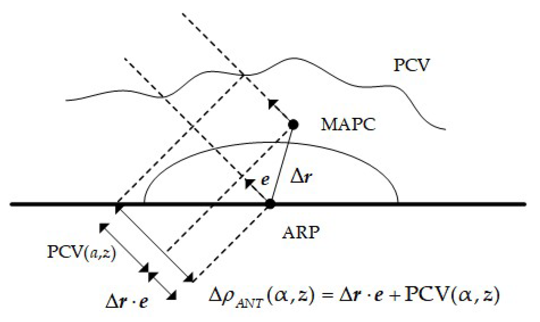
2.3. Antenna Phase Center Variation Model

The phase center variation (PCV) of the receiver is mainly related to the azimuth angle α and altitude angle z of the observed GPS satellite; then, the equivalent range error Δ ρ A N T ( α , z ) caused by the correction of the phase center of the HY-2A satellite receiver antenna can be expressed as follows:
Δ ρ A N T ( α , z ) = Δ r e + PCV ( α , z )
where Δ r is the phase center offset (PCO) of the receiver antenna, which is the deviation vector between the mean antenna phase center (MAPC) and the antenna reference point (ARP), usually represented as a three-dimensional constant offset. PCV ( α , z ) represents the PCV correction value; e is the unit vector of the incident direction of the satellite signal, as shown in Figure 1.
For the PCO and PCV, ground calibration values are usually used as prior values, which are corrected during orbit determination [27]. In this paper, the PCO prior information obtained from the ground is regarded as a fixed value, with a focus on analyzing the impact of the PCV on the HY-2A POD.
The representation of the PCV model includes spherical harmonic functions and piecewise linear functions [28]. Spherical harmonic functions provide a clear physical interpretation of the PCV but involve a larger computational load. In contrast, the piecewise linear function model is widely used because of its small computation and easy implementation. In this paper, the piecewise linear function method is chosen to represent the PCV model. It involves dividing the model based on elevation angle and azimuth angle into a grid and utilizing bilinear interpolation to calculate the corresponding PCV for a given elevation and azimuth angles. Assuming the four sought-after grid points are labeled as ( α i , z j ) , ( α i + 1 , z j ) , ( α i , z j + 1 ) , and ( α i + 1 , z j + 1 ) , as shown in Figure 2, the PCV value of point P in this grid is obtained through bilinear interpolation, expressed as follows:
PCV ( α , z ) = α α i α i + 1 α i [ PCV ( α i + 1 , z ) PCV ( α i , z ) ] + PCV ( α i , z )
PCV ( α i + 1 , z ) = z z j z j + 1 z j [ PCV ( α i + 1 , z j + 1 ) PCV ( α i + 1 , z j ) ] + PCV ( α i + 1 , z j )
PCV ( α i , z ) = z z j z j + 1 z j [ PCV ( α i , z j + 1 ) PCV ( α i , z j ) ] + PCV ( α i , z j )
where PCV ( α i , z j ) is the sought-after PCV parameter ( i = 1 , 2 , , m ; j = 1 , 2 , , n ) , and the values of m and n are dependent on the grid resolution.

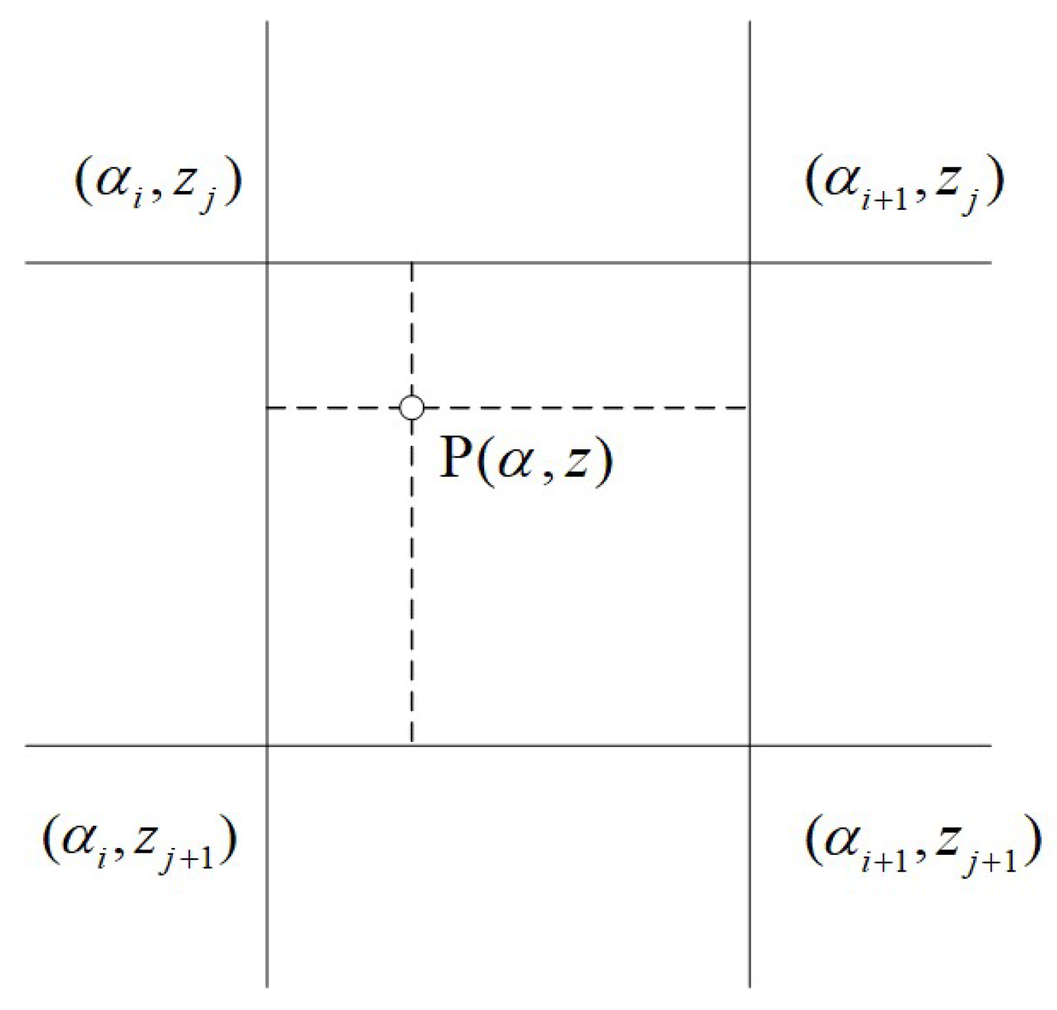
2.4. Methods for Estimating the Phase Center Variation Model

The main methods for the PCV estimation of LEO satellites include the direct method and residual method. The direct method [29] involves introducing the unknown parameter PCV into the orbit determination observation equation and solving it simultaneously with other parameters to be estimated.
The pseudo-range and carrier phase observations of the two frequencies of L1 and L2 received by the HY-2A constitute the ionosphere-free combination, respectively. The observation equation can be expressed as follows:
P = A y + B p + C d t r + ε P Φ = A y + B p + C d t r + D a + ε Φ
where P is the pseudo-range ionosphere-free combination observation vector; Φ is the carrier phase ionosphere-free combination observation value; and y = a , e , i , Ω , ω , T 0 , a 0 , , a n T is the vector of six orbit parameters and empirical acceleration parameters to be estimated. A is the corresponding coefficient matrix; p is the PCV parameter vector; B is the corresponding coefficient matrix; d t r is the receiver clock bias parameter; C is the corresponding coefficient matrix; a is the ionosphere-free combination ambiguity parameter vector; D is the corresponding coefficient matrix; and ε P and ε Φ are the observation noises for the pseudo-range and carrier phase, respectively.
During PCV estimation, parameters such as satellite clock bias and ambiguity can be pre-eliminated before the parameter estimation [30]. According to the least squares principle, the normal equations containing orbit, empirical acceleration, and PCV parameters can be obtained as follows:
N x = U
where x = y p T ; N = H T Q - 1 H is the coefficient matrix of the normal equations; U = H T Q - 1 L is the free term vector of the normal equations; H is the design matrix corresponding to orbit parameters, empirical acceleration parameters, and PCV parameters; Q 1 is the corresponding weight matrix; and L is the corresponding constant term matrix.
The residual method [31] involves modeling the carrier phase residuals of different elevations and azimuth angles after precise orbit determination. The PCV value at a grid point is obtained by averaging the carrier phase-residuals in the small neighborhood around the grid point:
Δ PCV ( e ) = PCV true ( e ) PCV mode ( e )
where PCV true ( e ) is the true PCV model, PCV mode ( e ) is the employed PCV model, and Δ PCV ( e ) denotes the difference between them, representing the unmodeled error.
This error is directly reflected in the carrier phase observation residuals after orbit determination:
Δ PCV ( e ) Δ ( L IF Z IF )
where L IF represents the ionosphere-free combination observation and Z IF represents the model value after correcting for remaining errors (excluding PCV).
The use of the residual method in actual orbit determination is influenced by factors such as satellite clock bias and ambiguity parameters. Therefore, it is necessary to eliminate the influence of these errors through multiple iterations. Generally, three to five iterations are required to achieve convergence [32].
In this paper, the carrier phase residual of RD orbit determination from the satellite-borne GPS data of HY-2A satellite for 31 days from day of year (DOY) 191 to 221 in 2013 is used to estimate the 10° × 10° and 5° × 5° PCV model. In the process of POD using the PCV model estimated with the residual method, three iterations are performed to reach convergence.

2.5. Reduced-Dynamic Orbit Determination Strategies of HY-2A

In this study, the satellite-borne GPS observation data of the HY-2A from DOY 191 to 221 in 2013 are selected for POD (sampling interval 1 s), and the orbit arc length was 24 h. Based on the Bernese 5.2 platform, precise ephemeris and satellite clock products provided by CODE are used for RD orbit determination and for finding the best pseudo-stochastic pulse parameters. Five solutions are designed to determine the orbit of the HY-2A. Solution 1 involves RD orbit determination without estimating the PCV model. Solution 2 uses the direct method to estimate a 10° × 10° PCV model for RD orbit determination. Solution 3 uses the direct method to estimate a 5° × 5° PCV model for RD orbit determination. Solution 4 uses the 10° × 10° PCV model estimated using the residual method for RD orbit determination. Solution 5 uses the 5° × 5° PCV model estimated using the residual method for RD orbit determination. The orbit precision is evaluated by three methods, including carrier phase residual analysis, external PSO validation, and SLR 3D validation, respectively. Table 1 details the mechanical model, observation model, and estimated parameters used in the RD POD of the HY-2A.

3. Result and Analysis

3.1. Quality Analysis of Satellite-Borne GPS Observations

In this section, the satellite-borne GPS data from DOY 203 to 209 in 2013 are selected for the data quality analysis. And the performance of the experimental receiver is evaluated by satellite visibility, multipath effect, ionospheric delay, and rate of change of ionospheric delay.

3.1.1. Satellite Visibility

Satellite visibility is the number of satellites tracked by the receiver at the same epoch, which can indicate the performance of the receiver in tracking GPS satellites. Figure 3 depicts the distribution characteristics of the number of satellites observed by the HY-2A satellite’s receiver from DOY 203 to 209 in 2013. As can be seen from Figure 3, only 0.31% of epochs observe three or fewer GPS satellites, and more than 99.69% of the epochs can observe four or more GPS satellites. Additionally, more than 98.67% of epochs can observe five or more GPS satellites, and 91.68% of epochs can observe six or more GPS satellites. Furthermore, 72.79% of epochs can observe seven or more GPS satellites. It can be seen that the HY-2A satellite can track more than six satellites most of the time. On average, 7.7 GPS satellites are observed per epoch, which provides a substantial amount of observation data for orbit determination.

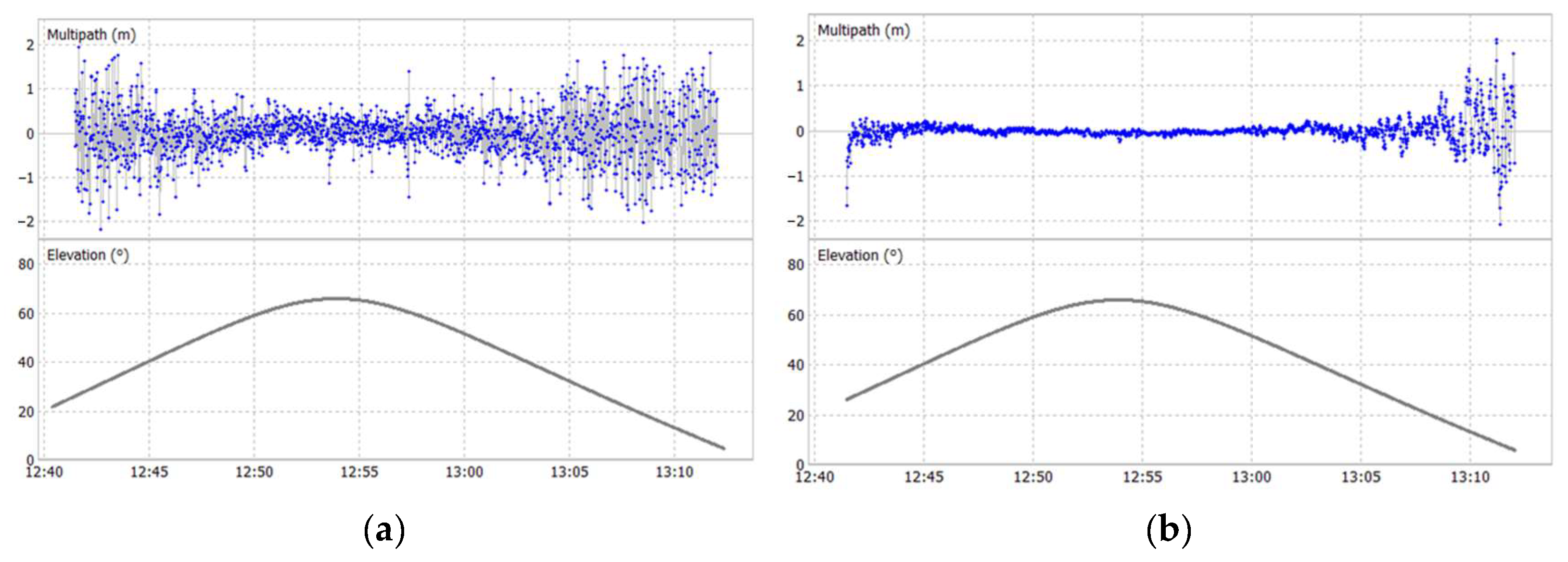
3.1.2. Multipath Effect

In GPS measurements, the signal (direct wave) received by the receiver from the satellite will be affected by the signal (reflected wave) reflected by the reflector, which will cause the observation values to deviate from the true values and introduce a multipath delay error [38]. The o/slps represents the ratio of the observed epoch of satellite-borne GPS data over a period of time to the epoch of the cycle slips. The cycle slip ratio of ground static observation data is generally greater than 200. However, due to the high-speed motion of the satellite-borne receiver, significant variations in ionospheric delay between adjacent epochs and environmental factors during operation can lead to GPS signal loss and more cycle slips. When the cycle slip is smaller, the cycle slip ratio is larger, so the observation quality is better. The data completeness rate is the ratio of the actual epochs observed by the satellite to the theoretical epochs over a period, and the data utilization rate is the ratio of epochs with complete observations to all observed epochs. The data completeness rate and utilization rate reflect the performance and availability of the satellite-borne receiver in acquiring data.
Table 2 summarizes the quality assessment results of the HY-2A satellite-borne observations. It evident from Table 2 that the mean root mean square (RMS) values of the L1 multipath error (MP1) is 42.4 cm, the mean RMS values of the L2 multipath error (MP2) is 32.7 cm, the mean cycle slip ratio is 45, and the data completeness rate and utilization rate are 98.19% and 93.56%, respectively.
Figure 4a,b illustrate the relationship between multipath effects and elevation angle for the L1 and L2 bands of the G03 satellite on DOY 203 in 2013. It can be seen from Figure 4 that the lower the elevation angle, the greater the multipath error. Additionally, the impact of low-elevation angles on MP1 is more significant. It is evident that during the initial and final stages of signal reception, the fluctuation of MP1 is noticeably greater than that of MP2. In the middle stage of signal reception, when the elevation angle is higher, both MP1 and MP2 values become smaller and more stable. Figure 4a shows the multipath error for the L1 band of G03 satellite, with MP1 fluctuating in the range of −2 to 2 m. When the satellite elevation angle is greater than 40°, the multipath error is small and smooth. On the contrary, MP1 fluctuates more significantly. Figure 4b displays the multipath error for the L2 band of G03 satellite, exhibiting larger fluctuations at the beginning of observations collection after the receiver locks onto the GPS satellite signal, which normalizes after a brief period. When the elevation angle is greater than 30°, MP2 consistently fluctuates in the range of −0.5 to 0.5 m.

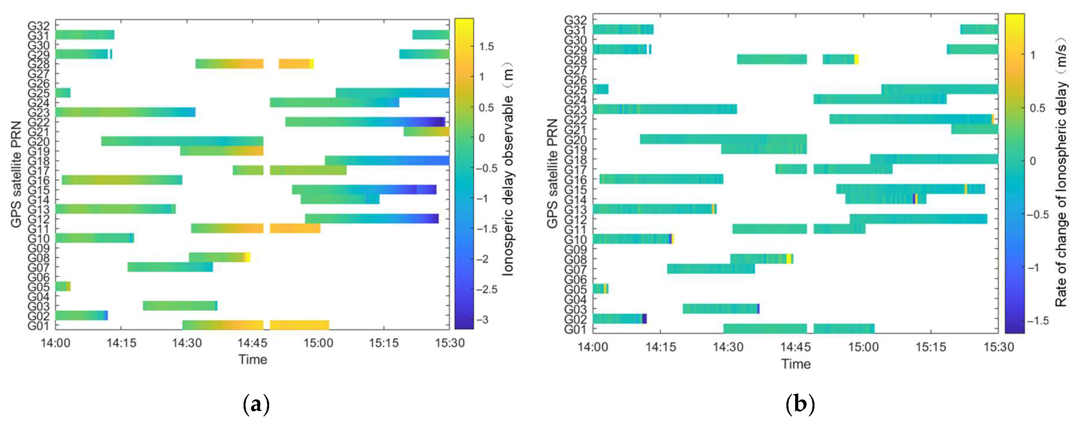
3.1.3. Ionospheric Delay and Rate of Change of Ionospheric Delay

When the satellite signal passes through the ionosphere, it is influenced by free ions and electrons, causing changes in propagation speed and path, thus affecting the signal propagation time. Therefore, the geometric distance between the satellite signal transmitter and the receiver will produce errors. When the propagation paths are the same, combining dual-frequency carrier observations allows for the determination of ionospheric delays I ion , 1 and I ion , 2 for the L 1 and L 2 bands [39]:
I ion , 1 = f 2 2 f 1 2 f 2 2 ( λ 1 N 1 λ 2 N 2 + M 1 M 2 ) = f 2 2 f 1 2 f 2 2 ( L 1 L 2 ) I ion , 2 = f 1 2 f 1 2 f 2 2 ( λ 1 N 1 λ 2 N 2 + M 1 M 2 ) = f 1 2 f 1 2 f 2 2 ( L 1 L 2 )
where L 1 and L 2 are carrier phase observations, f i represents carrier frequencies of L i , λ i represents wavelengths of L i , N i represents integer ambiguities of L i , and M i is the multipath error of L i , where i = 1, 2.
The rate of change of ionospheric delay is the variation of ionospheric delay per unit time. It can be obtained by differencing the ionospheric delays between two consecutive epochs as follows:
I O D 1 = I i o n , 1 j I i o n , 1 j 1 t j t j 1 I O D 2 = I i o n , 2 j I i o n , 2 j 1 t j t j 1
where I O D 1 and I O D 2 represent the ionospheric delay rate of L1 and L2, respectively, and t j represents the epoch j .
IOD indicates the activity level of the ionosphere. When the sampling interval is short and no cycle slips occur, the rate of change in ionospheric delay will be small. When IOD is >4 m/min, it can be considered that the ionosphere has undergone slips. In this paper, the cycle slip is differentiated by dual-frequency GPS carrier observation data. Figure 5a,b, respectively, show the ionospheric delay and the rate of change in ionospheric delay from 14:00 to 15:30 on DOY 203 in 2013. In Figure 5a, it can be found that the residual error of G01, G11, and G28 satellites is large from 14:30 to 15:00. The residual is large for satellites G12, G15, G18, and G22 in the range of 15:15 to 15:30. The residuals of other satellite observations are generally at a low level. In Figure 5b, brief abrupt changes in the rate of change in ionospheric delay (green to dark blue or yellow) at the end of the G02, G03, G08, G10, G13, G14, G22, and G28 satellites’ observation period can be observed, and this phenomenon is caused by the discontinuity or abnormal values of the carrier phase observations [40].

3.2. Impact of Pseudo-Stochastic Pulse on Reduced-Dynamic Orbit Determination

In the orbit determination process of the low-orbit satellite, the time intervals and a priori sigma of the pseudo-stochastic pulse are usually set according to experience. This study used different pseudo-stochastic pulse priors in the orbit determination process, and the results obtained were compared with the PSO provided by CNES. The PSO is determined using a combination of DORIS and GPS data, achieving an orbit precision of 2 to 3 cm [41]. In this experiment, the satellite-borne GPS data on DOY 204 in 2013 was selected; according to the HY-2A satellite’s orbital period (approximately 104 min), the time intervals are set to 6 min, 15 min, 30 min, and 60 min. The a priori sigma of R, T, and N components decreases gradually from the order of 1 × 10⁻⁴, specifically, 1 × 10⁻⁴ m/s2, 1 × 10⁻⁵ m/s2, 1 × 10⁻⁶ m/s2, 1 × 10⁻⁷ m/s2, 1 × 10⁻⁸ m/s2, and 1 × 10⁻⁹ m/s2. Table 3 shows the RMS values of the HY-2A for different pseudo-stochastic pulse time intervals and a priori sigma compared with the PSO.
In the process of LEO POD, although the perturbation force model can be used to express the perturbation force of the satellite to a certain extent, such as the non-central gravity of the Earth and the atmospheric drag, there are still some deviations in the perturbation force model [42] Therefore, the pseudo-random pulse parameter is introduced into the LEO POD to compensate the deviation of the mechanical model. Moreover, according to the characteristics of different satellites, the optimal pseudo-random pulse prior value of each satellite is different, considering the satellite altitude, perturbation model, and observation data quality.
From Table 3, at all-time intervals, when the a priori sigma is 1 × 10⁻⁸ m/s2, the orbit determination precision is the highest.
The influence of the change in the a priori sigma on the orbit precision is analyzed when the time interval is fixed. At the same time interval, when the a priori sigma ranges from 1 × 10⁻⁴ m/s2 to 1 × 10⁻⁷ m/s2, the orbit precision does not show significant variations. However, when the a priori sigma is further reduced to 1 × 10⁻⁸ m/s2, a noticeable improvement in mutual comparison precision is observed. Both the RMS values of R and 3D directions are minimized, indicating the highest orbit precision. Especially in the embodiment of the radial accuracy, the orbital precision has been significantly improved. For HY-2A satellite, the precision of the radial orbit is particularly important, and it affects the reliability of the altimetry task. Therefore, the reasonable selection of the optimal pseudo-stochastic pulse a priori value is very important for LEO POD. When the a priori sigma is further reduced from 1 × 10⁻⁸ m/s2 to 1 × 10⁻⁹ m/s2, there is a decline in orbit precision.
The influence of the change in the time intervals on the orbit precision is analyzed when the a priori sigma is fixed. It is observed that larger pseudo-stochastic pulse time intervals (30 and 60 min) result in poorer orbit precision. This is because the pseudo-pulse parameters are set too little, resulting in many unmodeled errors that cannot be effectively absorbed. Conversely, when the pseudo-pulse time interval is set to 6 min, the orbit precision also decreases, which may be due to the instability of orbit determination caused by too many pseudo-stochastic pulse parameters.
In conclusion, this study selects a pseudo-stochastic pulse time interval of 15 min and a priori sigma of 1 × 10⁻⁸ m/s2 for the experiment.

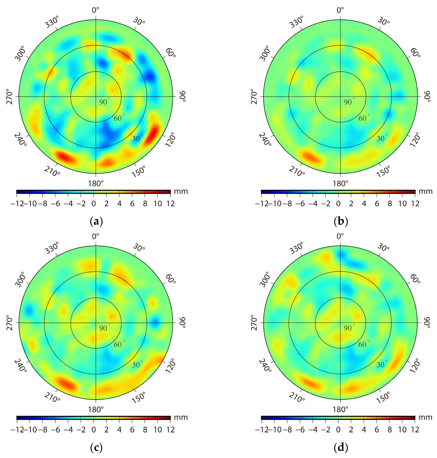
3.3. Estimation of the PCV Model

Figure 6 shows the 10° × 10° and 5° × 5° PCV models of HY-2A estimated using the direct method and residual method, respectively. From Figure 6, it is observed that the characteristics of the direct method and residual method for estimating the PCV model are as follows:
(1)
The direct method treats the PCV of grid points as an unknown parameter to be solved in the observation equation, resulting in a more detailed PCV estimation, and thus the estimated PCV map shows a spotted distribution. The residual method estimates the PCV by averaging the carrier phase residuals within the grid interval, resulting in similar PCV values for adjacent grid points and a mostly striped distribution in the PCV map.
(2)
The larger PCV values of the PCV model estimated using the direct method and residual method are all distributed within the low elevation grid space. This is mainly because the observation data are affected by the multipath effect at low altitude angles, which leads to poor observation data quality.
(3)
There is a significant decrease in the PCV value when the resolution of the PCV model estimated using the direct method is increased from 10° to 5°. This is because the increase in parameters makes the PCV model more refined; on the contrary, the improvement of resolution has relatively little effect on the residual method to estimate the PCV model.

3.4. Analysis of Orbit Precision for HY-2A

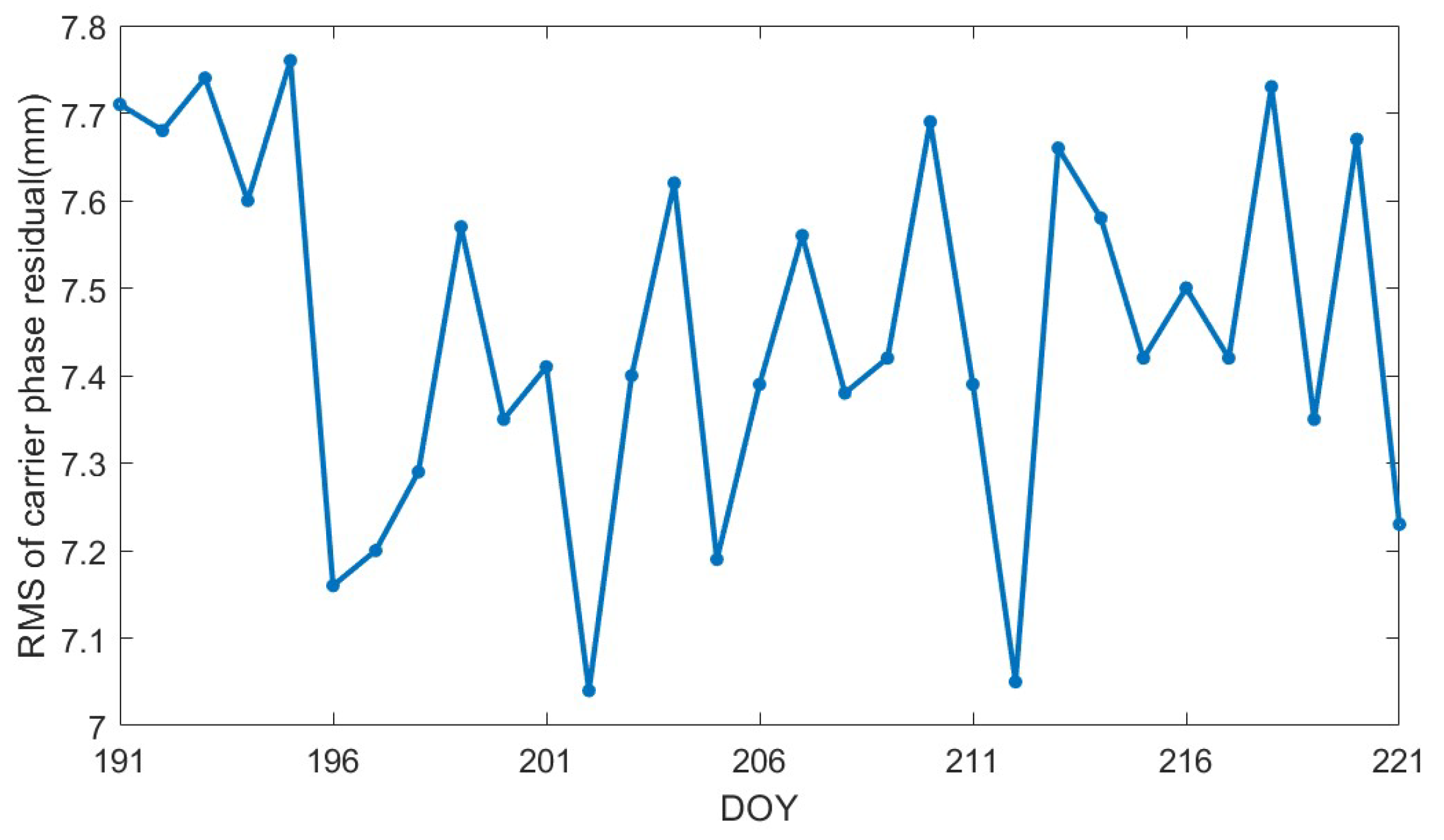
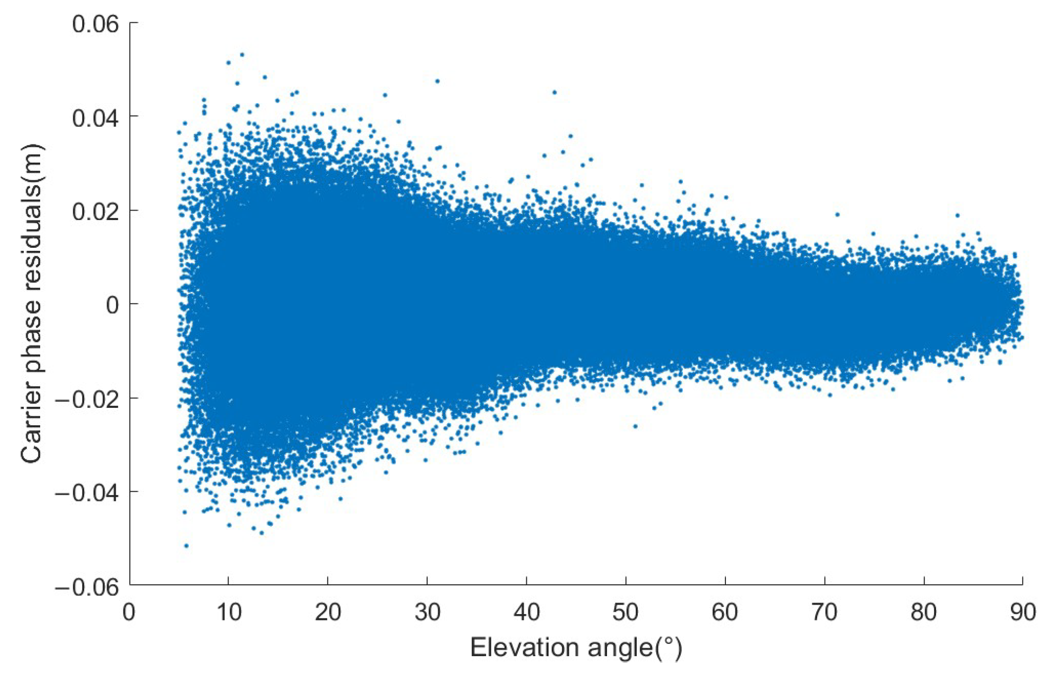
3.4.1. Carrier Phase Residuals Analysis

The carrier phase residual is one of the important indexes of orbit determination, which reflects the degree of fit between the observed data and the mechanical model used in orbit determination and the actual flight situation of the satellite. The quality of observation data, arc length of orbit determination, and parameters to be obtained are all important factors affecting the carrier phase residual [43]. The smaller the RMS value of carrier phase residuals, the higher the internal precision.
Figure 7 shows the RMS of carrier phase residuals for 31 days from DOY 191 to 221 in 2013 after selecting the optimal pseudo-stochastic pulse a priori values. From Figure 7, the RMS of the carrier phase residuals of a single day is in the range of 7.04 to 7.76 mm, and the fluctuation range is only 0.72 mm, with an average RMS value of 7.46 mm. The experimental results show that the mechanical model adopted in orbit determination is consistent with the actual situation. And the data obtained by the HY2 receiver is stable.
The specific sequence of the carrier phase residuals changing with elevation angle is illustrated in Figure 8; it can be observed that when the elevation angle is less than 20°, the carrier phase residuals are relatively large. The reason for this is the low elevation angle, which leads to the poor quality of observations. The carrier phase residuals for the HY-2A satellite fluctuated from −51.59 mm to 53.03 mm over the 31 days. Approximately 99.26% of the carrier phase residuals are distributed within the range of −25 mm to 25 mm, and the overall fluctuation is smooth, which indicates that the orbit determination strategy used in the course of orbit determination is reliable.

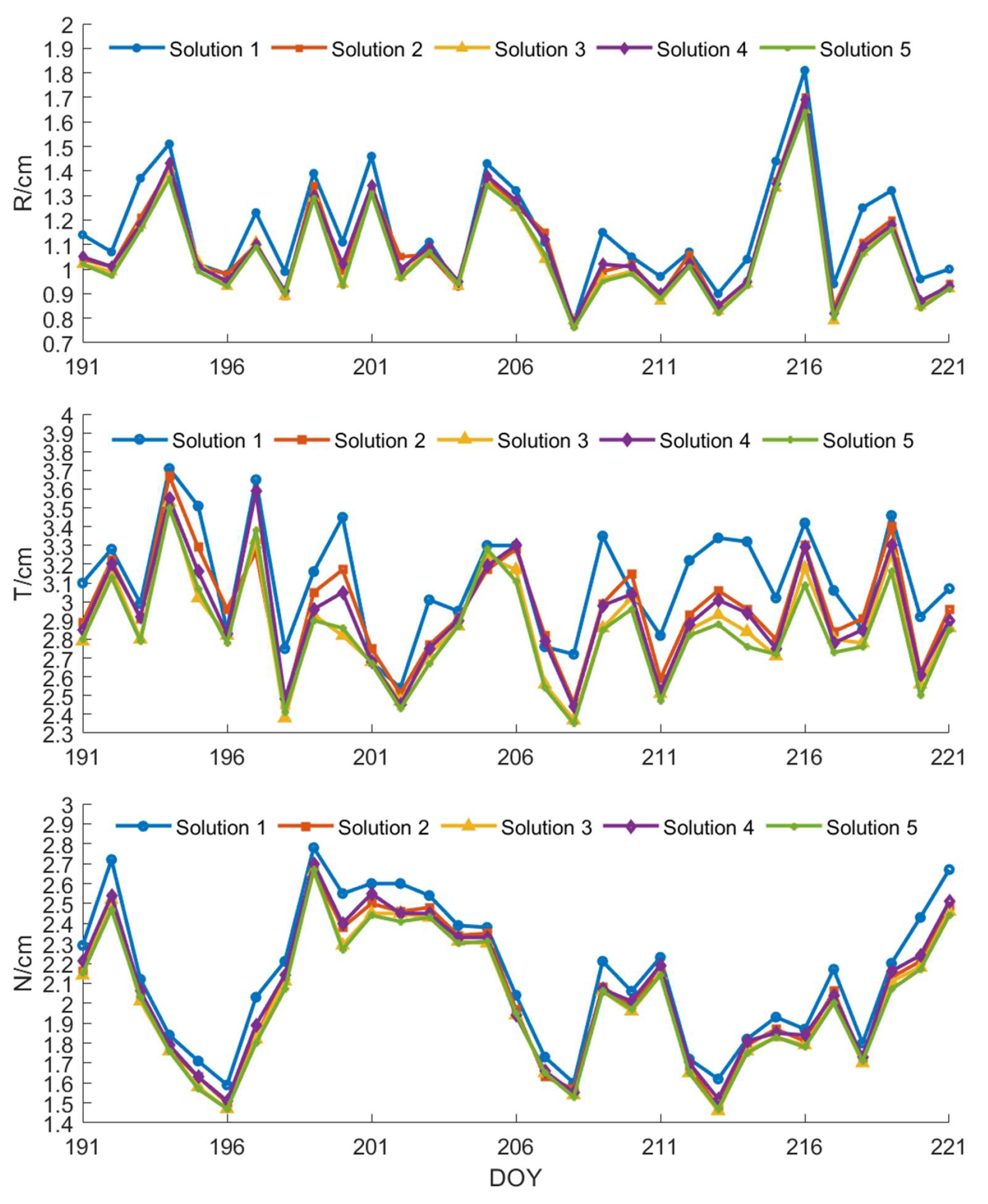
3.4.2. Comparison with Precision Science Orbits

The PSO provided by CNES is used as the reference orbit to evaluate the RD orbit precision of the HY-2A obtained in this experiment. Due to the fact that the orbit solution strategy and data provided by CNES are different from those in this study, it can be used for external validation. The precise orbit provided by CNES is referenced to International Atomic Time (TAI), while the standard orbit time system calculated in this experiment is based on GPS time (GPST) [44]. Therefore, it is necessary to pretreat the PSO in advance to unify the time system of the RD orbit. Figure 9 shows the RMS values in the R, T, and N directions of the residual difference between the RD orbit and the PSO of the HY-2A. Detailed statistical results can be found in Table 4.
As shown in Table 4, the orbit precision has been improved to different degrees after adding the PCV model. When the orbit is determined by Solution 1, the mutual comparison RMS values of the RD orbit with respect to the PSO in the R, T, N, and 3D directions are 1.15, 3.12, 2.14, and 3.96 cm, respectively. For Solution 2, compared to Solution 1, the RMS values for R, T, N, and 3D directions orbit comparisons decreased by 0.06, 0.14, 0.10, and 0.20 cm, respectively. For Solution 3, compared to Solution 1, the RMS values for R, T, N, and 3D directions orbit comparisons decreased by 0.09, 0.24, 0.13, and 0.29 cm, respectively. For Solution 4, compared to Solution 1, the RMS values for R, T, N, and 3D directions orbit comparisons decreased by 0.08, 0.17, 0.09, and 0.23 cm, respectively. Lastly, for Solution 5, compared to Solution 1, the RMS values for R, T, N, and 3D directions orbit comparisons decreased by 0.09, 0.27, 0.14, and 0.32 cm, respectively. The orbit precision of R, T, N, and 3D directions is significantly improved after adding the PCV model, and the PCV model of the HY-2A improves the precision of the poor tangential orbit more. The precision improvement brought by the improvement of PCV resolution is also higher in the tangential direction. The improvement in orbit precision brought by the increase in resolution is far less than the improvement after the addition of PCV model.
As shown in Figure 9, from an overall perspective, the RMS sequences of the R and N directions orbit residuals of the five solutions appear relatively smooth. However, the T direction orbit RMS value is a slightly larger fluctuation. The reason for this could be that the weak geometric constraints in the T direction are susceptible to large model errors [45]. The PCV models estimated using the direct method and residual method contribute to an improvement in orbit precision. The precision of the PCV models obtained from the direct method and residual method are comparable. The improvement of PCV model resolution has a greater effect on tangential orbit precision. When the resolution is increased from 10° to 5°, the orbit determination precision is further improved, but the improvement is small.

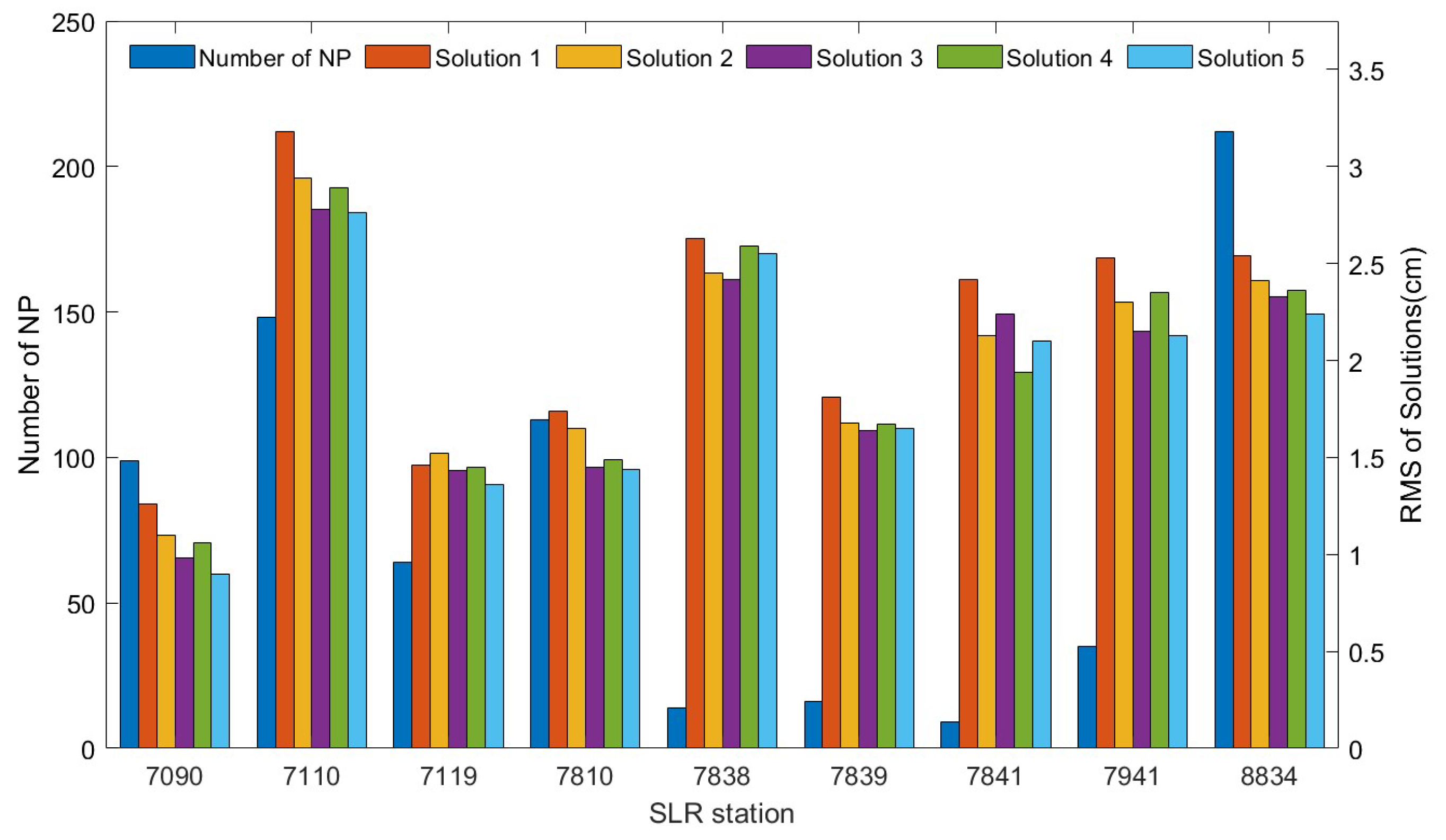
3.4.3. SLR 3D Validation

SLR data has extremely high precision, with a single ranging precision of better than 1 cm. At present, it is the most reliable method of tracking observation and LEO POD [6]. The SLR data for the HY-2A is supplied by the International Laser Ranging Service (ILRS) [46]. The SLR range validation involves comparing the distance between the station and the satellite obtained by SLR with the distance obtained by orbit determination.
During the period of DOY 191 to 221 in 2013, there were 12 SLR stations tracked by the HY-2A and 744 NP data were obtained. Among them, 7403, 7406, and 7825 stations were excluded due to poor quality or a small amount of observation data, with an exclusion rate of 4.70%. The remaining 709 NP data points were used for calculations, and the SLR orbit validation residuals were summarized. Figure 10 shows the NP data and RMS values of SLR station validation residuals for five solutions within 31 days. It can be seen that the 8834 station provided the most NP data, with 212 NP data points, accounting for 29.90% of the total data. When Solution 1 is used, the SLR range validation residual RMS value is 2.54 cm, which is improved by 0.13, 0.21, 0.18, and 0.30 cm, as compared with Solution 2, Solution 3, Solution 4, and Solution 5, respectively. The 7110 station obtained the poorest precision. When Solution 1 is used, the SLR range validation residual RMS value is 3.18 cm, which is improved by 0.24, 0.40, 0.29, and 0.42 cm, as compared with Solution 2, Solution 3, Solution 4, and Solution 5, respectively. The 7838, 7839, and 7841 stations provide relatively little NP data, and the improvement in the resolution of the PCV model is not obvious to the orbit precision. Overall, the majority of the stations achieved RMS values less than 3 cm, which meets the expected requirements.
SLR range validation only provides the range error and cannot evaluate orbit precision from the R, T, or N directions. Therefore, this paper improves on SLR range validation by transforming the one-dimensional SLR residuals into residual components in the R, T, and N directions. This is achieved by projecting the RTN unit vector onto the line-of-sight unit vector e. The unit vector formula e is as follows:
e = ( r R ) r R
where e is the line-of-sight unit vector, r is the satellite position, and R is the station position.
The specific implementation steps of SLR 3D validation are as follows:
(1)
Convert the PSO provided by CNES to the Bernese standard orbit format and convert it to a 1s sampling interval.
(2)
Calculate the station coordinates to the current epoch and transform the position and velocity of the HY-2A, along with the current epoch station coordinates, to the J2000 inertial system.
(3)
According to the time corresponding to each residual in the SLR residual file, the position and velocity of the HY-2A in the J2000 inertial system at that time and the station coordinates of that day are extracted.
(4)
The position and velocity of the HY-2A and the position of the station are converted from the J2000 inertial system to the position in the RTN coordinate system, and then the unit vector of the three directions of RTN is calculated according to Equation (16). Finally, the RTN residual component can be obtained by multiplying each SLR residual.
Table 5 shows the RMS values of the SLR validation residual components and distance residuals within 31 days. It can be seen that the precision is highest in the R direction, followed by the N direction, and the T direction. When Solution 1 was selected, the RMS values of the R, T, and N directions residual components of SLR 3D validation are 1.12 cm, 1.88 cm, and 1.29 cm, respectively. And the distance residual is 2.54 cm. When the PCV model resolution is increased from 10° to 5° using the direct method, the orbit precision in the R, T, and N directions is increased by 2.86%, 2.30%, and 2.50%, respectively. When the PCV model resolution is increased from 10° to 5° using the residual method, the orbit precision in the R, T, and N directions is increased by 1.90%, 2.96%, and 2.52%, respectively. The precision of PCV estimated using the direct method and residual method with different resolutions is improved, and the results are consistent with those obtained by the comparison of PSO provided by CNES.

4. Discussion

The HY-2A is China’s first marine dynamic environment monitoring satellite, and it has made great contributions to the successful launch and operation of HY2 series satellites. In order to ensure the smooth operation of the altimetry mission, it is equipped with the DORIS receiver, SLR receiver, and satellite-based GPS receiver. The performance of the receiver is mainly reflected in the data quality, which is one of the important factors affecting the orbit determination result. The HY2 receiver of the HY-2A is the first application in China. The quality of signals received by the HY2 receiver during in-orbit operation is analyzed from several indexes, which can provide a scientific basis for the subsequent development of satellite-borne GPS receivers.
In this paper, the impact of pseudo-random pulse and PCV model on the POD of the HY-2A is analyzed. In the process of RD orbit determination, the goal is to reasonably determine the pseudo-stochastic pulse time interval and a priori reasonably for different satellites. In most of the existing studies, the pseudo-stochastic parameters are determined by prior hypothesis or practical experience. The experiment found that the pseudo-stochastic pulse a priori value has a certain regulation effect on LEO POD. In addition, the CNES precision science orbit is selected as a reference to consider the R, T, N, and 3D directional precision. The error implied by the reference base itself is ignored, and the results are more convincing in later experiments using higher precision orbits or experiments using SLR.
Also, the PCV cannot be ignored in LEO POD. It is found that the PCV model estimated by the direct method is similar to that estimated by the residual method through the external PSO validation and SLR 3D validation, and the improvement in resolution has limited improvement on orbit precision. The 5° × 5°PCV grid model can meet most of the needs of POD [47], which also provides a reference for follow-up research. At the same time, the SLR 3D validation converts the distance residual into the residual in the direction of RTN, making the check results more intuitive and reliable, and can also be used for orbit checks of other satellites to enrich the orbit check system.

5. Conclusions

In this paper, TEQC is used to evaluate the quality of HY-2A satellite-borne GPS data from the satellite visibility, multipath effect, and ionospheric delay. The HY-2A satellite can observe 7.7 GPS satellites per epoch on average, and other indicators are normal. The result demonstrates that the experimental HY2 receiver, which was independently developed by China, has good signal capture performance. The regulating effect of pseudo-stochastic pulse a priori values on orbit precision was analyzed. The orbit precision of the HY-2A is the best when the pseudo-stochastic pulse time interval is 15 min, and the a priori sigma is 1 × 10⁻⁸ m/s2. The PCV models with different resolutions (10° × 10°, 5° × 5°) are estimated using the direct method and residual method, respectively, and introduced into the RD orbit determination process. The orbit obtained using the 10° × 10° PCV model and the 5° × 5° PCV model are more accurate than those without considering the PCV model. The carrier phase residual shows that the precision of inner coincidence has reached the centimeter level. The result of the external PSO validation and SLR 3D validation show that the influence of PCV on orbit determination results must be considered in the process of LEO POD. After adding the 5° × 5° PCV model using the residual method, the orbit precision in R, T, N, and 3D directions, compared with PSO, is improved by 8.49%, 9.47%, 7%, and 8.79%, respectively. And the results of SLR 3D validation are consistent with those obtained by the comparison of PSO provided by CNES.
According to the experimental results, the experimental HY2 receiver of the HY-2A can be applied to the mission of LEO POD. Although the pseudo-stochastic pulse can dynamically regulate the orbit precision, its regulation ability is limited. To obtain a high-precision orbit, it is not enough to only optimize the pseudo-stochastic pulse; in addition, various mechanical models and high-precision observation data need to be refined. The PCV is also one of the errors that must be considered in the process of POD; the orbit precision is further improved when the resolution is increased from 10° to 5°. The relevant experiments of the HY-2A can provide a useful reference for the POD of HY2 series satellites.

Author Contributions

Conceptualization, writing—original draft preparation, writing—review and editing, and methodology, J.G. and Y.W.; validation, Y.W. and S.Y.; formal analysis, X.C., Y.J., H.G. and X.L.; resources, Y.J.; data curation, H.G. and X.L.; funding acquisition, J.G. All authors have read and agreed to the published version of the manuscript.

Funding

The authors thank the National Satellite Ocean Application Center for providing data support. The study is partially supported by the National Natural Science Foundation of China (grant Nos. 42274006 and 42174041).

Data Availability Statement

Our sincere thanks go to the National Satellite Ocean Application Center for providing satellite-borne GPS data for HY-2A, CODE for providing GPS satellite orbits, clocks, and Earth rotation parameters, and the ILRS for providing SLR station data and SLR tracking data.

Conflicts of Interest

The authors declare no conflicts of interest.

References

  1. Yang, B.H. Constructing China’s ocean satellite system to the capability of ocean environment and disaster enhance monitoring. Chinese Space Sci. Technol. 2011, 31, 8. [Google Scholar]
  2. Zhang, Q.; Zhang, J.; Zhang, H.; Wang, R.; Jia, H. The study of HY2A satellite engineering development and in-orbit movement. Eng. Sci. 2013, 80, 12–18. [Google Scholar]
  3. Lin, M.S.; Zhang, Y.G.; Yuan, X.Z. The development course and trend of ocean remote sensing satellite. Haiyan Xuebao 2015, 37, 1–10. [Google Scholar]
  4. Cerri, L.; Berthias, J.; Bertiger, W.; Haines, B.; Lemoine, F.; Mercier, F.; Ries, J.C.; Willis, P.; Zelensky, N.; Ziebart, M. Precision orbit determination standards for the Jason series of altimeter missions. Mar. Geod. 2010, 33, 379–418. [Google Scholar] [CrossRef]
  5. Cazenave, A.; Hamlington, B.; Horwath, M.; Barletta, V.R.; Benveniste, J.; Chambers, D.; Döll, P.; Hogg, A.E.; Legeais, J.F.; Merrifield, M.; et al. Observational requirements for long-term monitoring of the global mean sea level and its components over the altimetry era. Front. Mar. Sci. 2019, 6, 582. [Google Scholar] [CrossRef]
  6. Guo, J.Y.; Wang, Y.C.; Shen, Y.; Liu, X.; Sun, Y.; Kong, Q.L. Estimation of SLR station coordinates by means of SLR measurements to kinematic orbit of LEO satellites. Earth Planets Space 2018, 70, 201. [Google Scholar] [CrossRef]
  7. Zhou, C.C.; Zhong, S.M.; Peng, B.B.; Ou, J.K.; Zhang, J.; Chen, R.J. Real-time orbit determination of Low Earth orbit satellite based on RINEX/DORIS 3.0 phase data and spaceborne GPS data. Adv. Space Res. 2020, 66, 1700–1712. [Google Scholar] [CrossRef]
  8. Kong, Q.L.; Guo, J.Y.; Sun, Y.; Zhao, C.M.; Chen, C.F. Centimeter-level precise orbit determination for the HY-2A satellite using DORIS and SLR tracking data. Acta Geophys. 2017, 65, 1–12. [Google Scholar] [CrossRef]
  9. Zhou, X.H.; Wang, X.H.; Zhao, G.; Zhao, G.; Peng, H.L.; Wu, B. The precise orbit determination for HY2A satellite using GPS, DORIS and SLR data. Geomat. Inf. Sci. Wuhan Univ. 2015, 40, 1000–1005. [Google Scholar]
  10. Zhu, J.; Wang, J.; Chen, J.; He, Y. Centimeter precise orbit determination for HY-2 via DORIS. J. Astronaut. 2013, 34, 163–169. [Google Scholar]
  11. Zhao, X.L.; Zhou, S.S.; Ci, Y.; Hu, X.G.; Cao, J.F.; Chang, Z.Q.; Tang, C.P.; Guo, D.N.; Guo, K.; Liao, M. High-precision orbit determination for a LEO nanosatellite using BDS-3. GPS Solut. 2020, 24, 102. [Google Scholar] [CrossRef]
  12. Kang, Z.; Tapley, B.D.; Bettadpur, S.; Ries, J.C.; Nagel, P.; Pastor, R. Precise orbit determination for the GRACE mission using only GPS data. J. Geod. 2006, 80, 322–331. [Google Scholar] [CrossRef]
  13. Švehla, D.; Rothacher, M. Kinematic positioning of LEO and GPS satellites and IGS stations on the ground. Adv. Space Res. 2005, 36, 376–381. [Google Scholar] [CrossRef]
  14. Mao, X.Y.; Arnold, D.; Girardin, V.; Villiger, A.; Jäggi, A. Dynamic GPS-based LEO orbit determination with 1 cm precision using the Bernese GNSS Software. Adv. Space Res. 2020, 67, 788–805. [Google Scholar] [CrossRef]
  15. Zhang, B.B.; Wang, Z.; Zhou, L.; Feng, J.; Qiu, Y.; Li, F. Precise orbit solution for swarm using space-borne GPS data and optimized pseudo-stochastic pulses. Sensors 2017, 17, 635. [Google Scholar] [CrossRef] [PubMed]
  16. Hwang, C.; Tseng, T.-P.; Lin, T.; Švehla, D.; Schreiner, B. Precise orbit determination for the FORMOSAT-3/COSMIC satellite mission using GPS. J. Geod. 2009, 83, 477–489. [Google Scholar] [CrossRef]
  17. Ijssel, J.; Visser, P.; Rodriguez, P. Champ precise orbit determination using GPS data. Adv. Space Res. 2003, 31, 1889–1895. [Google Scholar] [CrossRef]
  18. Xia, Y.W.; Liu, X.; Guo, J.Y.; Yang, Z.M.; Qi, L.H.; Ji, B.; Chang, X.T. On GPS data quality of GRACE-FO and GRACE satellites: Effects of phase center variation and satellite attitude on precise orbit determination. Acta Geod. Geophys. 2020, 56, 93–111. [Google Scholar] [CrossRef]
  19. Jäggi, A.; Dahle, C.; Arnold, D.; Bock, H.; Meyer, U.; Beutler, G.; van Den Ijssel, J. Swarm kinematic orbits and gravity fields from 18 months of GPS data. Adv. Space Res. 2016, 57, 218–233. [Google Scholar] [CrossRef]
  20. Guo, J.; Zhao, Q.; Guo, X.; Liu, X.; Liu, J.; Zhou, Q. Quality assessment of onboard GPS receiver and its combination with DORIS and SLR for Haiyang 2A precise orbit determination. Sci. China Earth Sci. 2015, 58, 138–150. [Google Scholar] [CrossRef]
  21. Lin, M.S.; Wang, X.H.; Peng, H.L.; Zhao, Q.L.; Li, M. Precise orbit determination technology based on dual-frequency GPS solution for HY-2 satellite. Eng. Sci. 2014, 16, 97–101. [Google Scholar]
  22. Guo, J.; Zhao, Q.L.; Li, M.; Hu, Z.G. Centimeter level orbit determination for HY2A using GPS data. Geomat. Inf. Sci. Wuhan Univ. 2013, 38, 52–55. [Google Scholar]
  23. Guo, J.Y.; Qi, L.H.; Liu, X.; Chang, X.T.; Ji, B.; Zhang, F.Z. High-order ionospheric delay correction of GNSS data for precise reduced-dynamic determination of LEO satellite orbits: Cases of GOCE, GRACE, and SWARM. GPS Solut. 2023, 27, 13. [Google Scholar] [CrossRef]
  24. Montenbruck, O.; Garcia-Fernandez, M.; Yoon, Y.; Schön, S.; Jäggi, A. Antenna phase center calibration for precise positioning of LEO satellites. GPS Solut. 2009, 13, 23–34. [Google Scholar] [CrossRef]
  25. Beutler, G.; Brockmann, E. Extended orbit modeling techniques at the CODE processing center of the international GPS service for geodynamics (IGS): Theory and initial results. Manuscr. Geod. 1994, 19, 367–386. [Google Scholar]
  26. Vaclavovic, P.; Dousa, J. G-Nut/Anubis: Open-Source Tool for Multi-GNSS Data Monitoring with a Multipath Detection for New Signals, Frequencies and Constellations. In Gravity, Geoid and Earth Observation; Springer: Cham, Switzerland, 2015; Volume 143, pp. 775–782. [Google Scholar]
  27. Liu, M.M.; Yuan, Y.B.; Ou, J.K.; Chai, Y.J. Research on attitude models and antenna phase center correction for Jason-3 Satellite orbit determination. Sensors 2019, 19, 2408. [Google Scholar] [CrossRef] [PubMed]
  28. Schmid, R.; Rothacher, M.; Thaller, D.; Steigenberger, P. Absolute phase center corrections of satellite and receiver antennas. GPS Solut. 2005, 9, 283–293. [Google Scholar] [CrossRef]
  29. Jäggi, A.; Dach, R.; Montenbruck, O.; Hugentobler, U.; Bock, H.; Beutler, G. Phase center modeling for LEO GPS receiver antennas and its impact on precise orbit determination. J. Geod. 2009, 83, 1145–1162. [Google Scholar] [CrossRef]
  30. Tian, Y.G.; Hao, J.M. Swarm satellite antenna phase center correction and its influence on the precision orbit determination. Acta Geod. Cartogr. Sin. 2016, 45, 1406–1412. [Google Scholar]
  31. Gu, D.; Lai, Y.; Liu, J.; Ju, B.; Tu, J. Spaceborne GPS receiver antenna phase center offset and variation estimation for the Shiyan 3 satellite. Chin. J. Aeronaut. 2016, 29, 1335–1344. [Google Scholar] [CrossRef]
  32. Mao, X.; Visser, P.N.A.M.; van den IJssel, J. Impact of GPS antenna phase center and code residual variation maps on orbit and baseline determination of GRACE. Adv. Space Res. 2017, 59, 2987–3002. [Google Scholar] [CrossRef]
  33. Pavlis, N.K.; Holmes, S.A.; Kenyon, S.C.; Factor, J.K. The development and evaluation of the Earth Gravitational Model 2008 (EGM2008). J. Geophys. Res. Solid Earth 2012, 117, B04406. [Google Scholar] [CrossRef]
  34. Ivantsov, A.V. Dynamical model of motion for asteroids based on the DE405 theory. Kinemat. Phys. Celest. Bodies 2007, 23, 65–69. [Google Scholar] [CrossRef]
  35. Luzum, B.; Petit, G. The IERS conventions (2010): Reference systems and new models. Proc. Int. Astron. Union 2012, 10, 227–228. [Google Scholar] [CrossRef]
  36. Rim, H.J. TOPEX Orbit Determination Using GPS Tracking System. Ph.D. Thesis, University of Texas at Austin, Austin, TX, USA, 1992. [Google Scholar]
  37. Lyard, F.H.; Allain, D.J.; Cancet, M.; Carrère, L.; Picot, N. FES2014 global ocean tide atlas: Design and performance. Ocean Sci. 2021, 17, 615–649. [Google Scholar] [CrossRef]
  38. Schreiter, L.; Montenbruck, O.; Zangerl, F.; Siemes, C.; Arnold, D.; Jäggi, A. Bandwidth correction of Swarm GPS carrier phase observations for improved orbit and gravity field determination. GPS Solut. 2021, 25, 70. [Google Scholar] [CrossRef] [PubMed]
  39. Estey, L.H.; Meertens, C.M. TEQC: The Multi-Purpose Toolkit for GPS/GLONASS Data. GPS Solut. 1999, 3, 42–49. [Google Scholar] [CrossRef]
  40. Hwang, C.; Tseng, T.-P.; Lin, T.-J.; Švehla, D.; Hugentobler, U.; Chao, B.F. Quality assessment of FORMOSAT-3/COSMIC and GRACE GPS observables: Analysis of multipath, ionospheric delay and phase residual in orbit determination. GPS Solut. 2009, 14, 121–131. [Google Scholar] [CrossRef]
  41. Arnold, D.; Montenbruck, O.; Hackel, S.; Sośnica, K. Satellite laser ranging to low Earth orbiters: Orbit and network validation. J. Geod. 2018, 93, 2315–2334. [Google Scholar] [CrossRef]
  42. Männel, B.; Rothacher, M. Geocenter variations derived from a combined processing of LEO- and ground-based GPS observations. J. Geod. 2017, 91, 933–944. [Google Scholar] [CrossRef]
  43. Guo, J.Y.; Wang, G.Z.; Guo, H.Y.; Lin, M.S.; Peng, H.L.; Chang, X.T.; Jiang, Y.M. Validating precise orbit determination from Satellite-Borne GPS data of Haiyang-2D. Remote Sens. 2022, 14, 2477. [Google Scholar] [CrossRef]
  44. Guo, H.Y.; Guo, J.Y.; Yang, Z.M.; Wang, G.Z.; Qi, L.H.; Lin, M.S.; Peng, H.L.; Ji, B. On Satellite-Borne GPS data quality and reduced-dynamic precise orbit determination of HY-2C: A case of orbit validation with onboard DORIS data. Remote Sens. 2021, 13, 4329. [Google Scholar] [CrossRef]
  45. Hu, Z.G.; Zhao, Q.L.; Guo, J.; Liu, J.N. Research on Impact of GPS phase center variation on precise orbit determination of low earth orbit satellite. Acta Geod. Cartogr. Sin. 2011, 40, 34–38. [Google Scholar]
  46. Pearlman, M.; Degnan, J.; Bosworth, J. The international laser ranging service. Adv. Space Res. 2002, 30, 135–143. [Google Scholar] [CrossRef]
  47. Yuan, J.; Zhao, C.; Wu, Q. Phase center offset and phase center variation estimation in-flight for ZY-3 01 and ZY-3 02 space-borne GPS antennas and the influence on precision orbit determination. Acta Geod. Cartogr. Sin. 2018, 47, 672–682. [Google Scholar]
Figure 1. Schematic diagram of the receiver antenna phase center correction.
Remotesensing 16 01336 g001
Figure 2. Schematic diagram of PCV grid linear interpolation of HY-2A.
Remotesensing 16 01336 g002
Figure 3. Number of satellites observed per epoch of HY-2A.
Remotesensing 16 01336 g003
Figure 4. Multipath effects and elevation angle changes for G03 satellite in L1 (a) and L2 (b).
Remotesensing 16 01336 g004
Figure 5. Ionospheric delay (a) and rate of change of ionospheric delay (b) of HY-2A.
Remotesensing 16 01336 g005
Figure 6. PCV model of HY-2A. (a) 10° × 10° PCV model using direct method; (b) 5° × 5° PCV model using direct method; (c) 10° × 10° PCV model using residual method; (d) 5° × 5° PCV model using residual method.
Remotesensing 16 01336 g006
Figure 7. RMS of carrier phase residuals of HY-2A within 31 days.
Remotesensing 16 01336 g007
Figure 8. Carrier phase residual sequence within 31 days.
Remotesensing 16 01336 g008
Figure 9. Line chart of RMS of the reduced-dynamic orbit and precision science orbit comparison in different solutions within 31 days.
Remotesensing 16 01336 g009
Figure 10. NP data and RMS of SLR station range validation residuals.
Remotesensing 16 01336 g010
Table 1. Reduced-dynamic orbit determination strategy of HY-2A.
Model/ParametersDescription
Mechanical modelGlobal gravity feld modelEGM2008 [33], 120 × 120
N-bodyJPL DE405 [34]
Solid earth tidesIERS2010 [35]
Solar radiation pressureBox-Wing [36]
Ocean tidesFES2004 [37]
Observation modelGPS dataUndifferenced ionosphere-free phase and code (interval 1 s)
GPS orbitsPost-processed precise orbit provided by CODE
GPS clockPost-processed precise clock corrections provided by CODE (time interval 30 s)
POD arc length24 h
SLRNormal Point (NP) data provided by ILRS
Attitude modelProvided by the NSOAS
GPS Satellite antenna phase modelPCV.I08
HY-2A PCVCalibrations in orbit
Elevation cutoff
Estimated parametersInitial state of orbit segment3-D inertial system position and velocity
Receiver clock offsetEpoch estimation
AmbiguityEach satellite, each observation arc, float solution
R, T, N empirical forceEstimated every 240 min
Pseudo-stochastic pulse priori sigma1 × 10−4 m/s2, 1 × 10⁻⁵ m/s2, 1 × 10⁻⁶ m/s2, 1 × 10⁻⁷ m/s2, 1 × 10⁻⁸ m/s2, 1 × 10⁻⁹ m/s2
Pseudo-stochastic pulse time interval6 min, 15 min, 30 min, 60 min
Table 2. Quality assessment statistics of HY-2A.
DOYMP1 RMS (cm)MP1 RMS (cm)O/slipCompleteness RateUtilization Rate
20341.031.14195.40%94.12%
20438.931.04599.55%93.97%
20544.332.13998.31%93.02%
20644.534.04699.25%93.51%
20741.332.54295.05%93.58%
20841.730.84499.84%93.70%
20940.932.04999.95%93.02%
Mean42.432.74598.19%93.56%
Table 3. RMS values of different pseudo-stochastic pulse time intervals and priori sigma deviations compared with precision science orbits (cm).
Priori Sigma (m/s2)Direction of
Orbit Comparison
Time Interval/min
6153060
1 × 10⁻⁴R0.960.960.960.97
T3.012.992.993.04
N2.432.432.442.42
3D3.993.973.974.00
1 × 10⁻⁵R0.970.970.960.96
T2.962.982.973.02
N2.442.422.432.41
3D3.963.963.963.98
1 × 10⁻⁶R0.960.960.970.97
T3.023.002.993.01
N2.422.412.412.42
3D3.993.963.973.98
1 × 10⁻⁷R0.950.950.960.96
T2.982.962.982.98
N2.432.422.412.41
3D3.953.943.963.96
1 × 10⁻⁸R0.930.930.940.94
T3.012.952.952.97
N2.392.392.412.43
3D3.943.913.933.95
1 × 10⁻⁹R0.950.940.950.95
T3.023.013.003.01
N2.422.402.432.43
3D3.993.963.983.99
Table 4. RMS of reduced-dynamic orbit and precision science orbit comparison in different solutions within 31 days (cm).
SolutionsRTN3D
Solution 11.153.122.143.96
Solution 21.092.962.043.76
Solution 31.062.882.013.67
Solution 41.072.952.053.73
Solution 51.062.852.003.64
Table 5. RMS of SLR 3D validation residuals components and distance residuals within 31 days (cm).
SolutionsRTNRes
Solution 11.121.881.292.54
Solution 21.081.781.232.41
Solution 31.051.741.202.35
Solution 41.071.741.222.38
Solution 51.051.691.192.32
Disclaimer/Publisher’s Note: The statements, opinions and data contained in all publications are solely those of the individual author(s) and contributor(s) and not of MDPI and/or the editor(s). MDPI and/or the editor(s) disclaim responsibility for any injury to people or property resulting from any ideas, methods, instructions or products referred to in the content.

