Abstract
Speckle noise and the spatial resolution of the Sentinel−1 Synthetic Aperture Radar (SAR) image can cause significant difficulties in the detection of small objects, such as small ships. Therefore, in this study, the Polarimetric Combination-based Ship Detection (PCSD) approach is proposed for enhancing small ship detection performance, which combines three different characteristics of polarization: newVH, enhanced VH, and enhanced VV. Employing the Radar Cross Section (RCS) value in three stages, the newVH was utilized to detect Automatic Identification System (AIS) -ships and small ships. In the first step, the adaptive threshold (AT) method was applied to newVH with a high RCS condition (>−10.36 (dB)) for detecting AIS-ships. Secondly, the first small ship target was detected with the maximum suppression of false alarms by using the AT with a middle RCS condition (>−16.98 (dB)). In the third step, a candidate group was identified by applying a condition to the RCS values (>−23.01 (dB)), where both small ships and speckle noise were present simultaneously. Subsequently, the enhanced VH and VV polarizations were employed, and an optimized threshold value was selected for each polarization to detect the second small ship while eliminating noise pixels. Finally, the results were evaluated using the AIS and small fishing vessel tracking system (V-Pass) based on the detected ship positions and ship lengths. The average matching results from 26 scenes in 2022 indicated a matching rate of over 86.67% for AIS-ships. Regarding small ships, the detection performance of PCSD was 42.27%, which was over twice as accurate as the previous Constant False Alarm Rate (CFAR) ship detection model. As a result, PCSD enhanced the detection rate of small ships while maintaining the capacity for detecting AIS-equipped ships.
1. Introduction
Synthetic Aperture Radar (SAR) satellites employ coherent microwave sensors to capture the earth’s surface, and SAR data are widely utilized for ocean surveillance. The key advantages of SAR satellites lie in their ability to capture images with high resolution under various lighting conditions (day–night imaging capability) and their ability to penetrate through clouds, which makes them exceptionally valuable for versatile marine surveillance fields. The marine surveillance fields include the detection and tracking of marine vessels and marine pollutants such as oil spills, macroalgal blooms, etc. In the case of tracking maritime vessel activities, the Automatic Identification System (AIS) is widely recognized as a major Vessel Monitoring System (VMS); nevertheless, its coverage is limited, rendering it challenging to gather comprehensive ship surveillance data. Therefore, SAR-based ship detection can aid in this traditional ship monitoring system. Despite their many benefits, SAR data nevertheless have certain drawbacks, such as a significant discontinuity in monitoring and speckle noise. While a target such as a ship with a high backscattering value might be promptly detected, a ship with a low backscatter value might be challenging to distinguish from a speckle noise with a similar value [1]. Therefore, to improve the performance of SAR-sensor-based ship detection, windowing-based target detection techniques and artificial intelligence technologies like deep learning (DL) methods are being widely used. In particular, Convolutional Neural Networks (CNNs) and CNN-based object detection approaches are useful ways to analyze images and extract features, making them suitable for studies related to the detection of marine vessels.
Several experimental studies have been conducted to detect ships from the SAR data on the basis of the Region-based CNN (RCNN), Single Shot Multi Box Detector (SSDD), and You Only Look Once (YOLO) algorithms, which are frequently used as part of object detection [2,3,4,5]. In particular, Ref. [6] attempted to develop a DL algorithm for detecting small targets as an experimental challenge. However, the results appeared to have limited applicability due to the insufficient quantity and quality of the dataset. These deficiencies were addressed by generating a ship detection dataset utilizing long-term data from a variety of SAR platforms [7,8,9]. Although the models developed here strengthened the dataset’s reliability, they needed to account for the polarimetric characteristics provided by SAR microwaves since they analyzed SAR satellites using only basic input images, which represents the simplest approach to managing the data for DL applications. The second approach, which is the most widely used windowing-based ship detection method, employs a Constant False Alarm Rate (CFAR) detector to detect targets with higher backscattering values than their surroundings [10]. In particular, Ref. [11] proposed an optimal ship detection approach to detect ships from Sentinel−1 images on the basis of various CFAR methods and parameter adjustments. Furthermore, before implementing CFAR, several techniques have been proposed to either eliminate noise or improve the input data so that they can be used for ship detection, hence enabling the detection of a specific ship [1,12,13]. However, since this approach overlooks polarimetric characteristics as well, noise in the image itself may result in false ship detection. To overcome this, a ship detection method was proposed on the basis of CFAR that considers the specialized characteristics of various SAR sensors. Specifically, since multiple polarizations are typically provided in SAR, it is feasible to generate a new polarized image through a transformation that can be used to detect ships or analyze the cross-correlation of polarizations by combining two or more polarized images instead of just one [14,15,16,17,18,19]. Furthermore, Ref. [20] reduced the number of false positives caused by azimuth ambiguity by employing the helix scattering approach. However, since these studies deal with a limited number of sample ships in a particular region, they are often considered unreliable. In addition, to enhance the ship detection performance, Ref. [21] used the dual-polarized Sentinel−1 image and proposed a method for reducing false alarms by combining the co- and cross-polarized images. Ref. [22] provided a good ship detection performance for each dual-pol after comparing a significant number of ship detection results with AIS. However, its detection capabilities for small ships remain limited as it is solely studied for AIS.
As a result, a ship detection algorithm designed for a particular ship type was proposed, which included selecting a specific small ship as a target along with employing CFAR and different polarizations [23,24,25]. Furthermore, Refs. [26,27] prepared test vessels, such as thin inflated rubber ships and refugee vessels, directly and proposed an optimal vessel detection method for multiple satellite platforms. However, as the satellite platforms and polarization images differ, an optimal coefficient setting was required for application to this study. Thus, by combining multiple polarization images and using an adaptive threshold approach, this study proposed a method to improve the detection performance of small ships.
Our contributions include the following:
- Both polarizations (VH and VV) of Seninel−1 SAR’s were used to generate three new polarimetric images that were denoted as newVH, enhanced VH, and enhanced VV, and a vessel detection approach was independently applied to these three images. We proposed a method to separately detect the AIS-ships and the first SM-ships (small ships) from the newVH image by selecting two distinct threshold conditions, and then using the adaptive threshold method. Afterwards, a threshold condition was employed in the newVH to detect the candidate small ships. To detect the remaining small ships (second SM-ships) from the candidates, an optimal individual threshold was applied to the enhanced VH and enhanced VV images independently which eliminate the noise from the candidates. As a result, small ships with a low false positive rate were detected individually, while a high detection performance for AIS-ships was also maintained.
- The results of the ship detection were compared with ship information from the AIS/V-pass (small fishing vessel tracking system) ground truth, and long-term data were also employed to provide highly reliable assessment information. Additionally, by improving the AIS/V-Pass ship location information and compensating for the azimuth shifting phenomenon that occurs in satellites, the matching accuracy was improved.
The remaining sections of this article are organized as follows:
In Section 2, the spatial area of the study and the satellite images, AIS, V-Pass information, and environmental data used in this study are presented. Additionally, satellite image preprocessing, AIS/V-Pass vessel information correction, and small vessel detection enhancement methods are explained in detail. Section 3 presents example results for one test set and ship detection application and evaluation results for the entire period. Section 4 includes a discussion of the results along with the outcomes from the other methods. And finally, Section 5 presents the conclusion of this work.
2. Materials and Methods
2.1. Study Area and Data
In this study, Sentinel−1 Ground Range Detected High Resolution (GRDH) images and AIS and V-Pass data were used. Sentinel−1 images were utilized for ship detection purposes, which are publicly available and obtained from the Copernicus website (https://scihub.copernicus.eu/, accessed on 3 March 2023), while AIS and V-pass were used to evaluate the detection results. Sentinel−1 dual-polarized images are considered to be high-resolution images with resolutions of 10 m and are widely used to detect various marine phenomena, such as ship detection, and they are also used for observational research [28,29]. Until 2021, Sentinel−1A and Sentinel−1B operated simultaneously, collecting data once a week in the research area. However, in 2022, only Sentinel−1A provided images due to the ageing of Sentinel−1B and the scheduled replacement in 2024, resulting in image acquisition every two weeks.
According to International Maritime Organization (IMO) standards, AIS, one of the VMS, must be installed on ships weighing more than 300 tons. On the other hand, V-Pass, developed by the Coast Guard of Korea, is installed on small fishing boats of 300 tons or less to monitor the small vessels that are not covered by AIS [30]. The two collection devices mentioned above were established and are being operated in real-time by the Korea Institute of Ocean Science and Technology (KIOST) in Yeongdo, Busan [31,32]. The receiving range of the vessel information is roughly 35 km [33], and it is collected every 1 to 3 min, depending on the sea conditions and the vessel gathering status. The vessel information comprises position, speed, course, and length. The research area is depicted in Figure 1. The transmitting range of the AIS that was used for evaluation was taken into consideration, which is why the Busan region was selected as the research area.
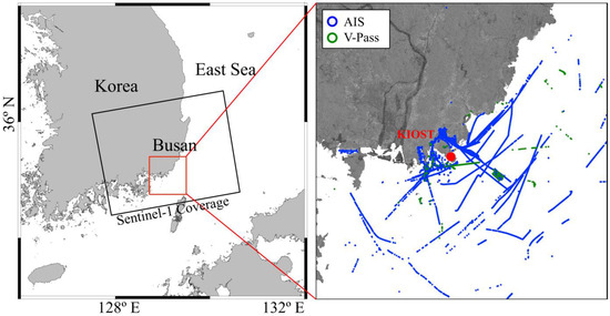
Figure 1.
Boundary of Sentinel−1 image (black rectangle) and study area (red rectangle) covering the Busan port (left). Ship trajectories from AIS (Automatic Identification System) and V-Pass (Small Fishing Vessel Tracking System) are displayed on the Sentinel−1 image obtained on 6 July 2022 (right). The trajectory data represents routes before and after 30 min of the Sentinel−1 image’s acquisition time (09:23:19 UTC).
All Sentinel−1 images of Busan from 1 January to 31 December 2022, were included in the dataset for ship detection. The total number of ships reported by AIS/V-Pass at each acquisition time is depicted in Table 1, and the total number of Sentinel−1 image was confirmed to be 26.

Table 1.
List of Sentinel−1 image used in this study with total number of ships observed by AIS/V-Pass during each data acquisition.
Additionally, to depict the wave trend at the ship position, meteorological modeling data for the study region were obtained from the Korea Operational Oceanographic System (KOOS), which include wave height and wind information. The data are provided in near real time at high resolution of up to 300 m at hourly intervals [34].
2.2. Methodology
Figure 2 depicts a schematic representation of the ship detection process from the Sentinel−1 multi-polarized data, where the results of ship detection were validated against the ship information obtained from the AIS/V-Pass data. Before applying the ship detection algorithm, radiometric terrain correction of the Sentinel−1 image was performed. Afterwards, according to the distinct characteristics of each image, a land masking map was generated by integrating satellite images with the ENC data. To improve the ship detection result, three new polarimetric images—newVH, enhanced VH, and enhanced VV—were created. Employing a global threshold poses challenges to detecting both AIS-ships and SM-ships. As a result, visual inspection was conducted for each image, and different thresholds for each ship target (AIS, V-Pass) were selected based on trial-and-error analysis. In the newVH image, multiple thresholding conditions were given for distinctly detecting the AIS-ships, first SM-ships and candidate SM-ships. Afterwards, enhanced VH and enhanced VV images were employed to detect the second SM-ships by conducting the filtering operation from the candidates, which contains both SM-ships and noise. Each detected ship chip image was utilized to calculate the ship length, which was then used for matching. The results of the ship detection were then evaluated. Based on the satellite acquisition time, the AIS/V-Pass location’s Dead Reckoning (DR) was determined, and the course and speed were interpolated. Furthermore, the azimuth shifting phenomenon—which results from the ship’s course and speed differing from that of the Sentinel−1 satellite platform—was taken into consideration when updating the position information of the ship. Finally, the proposed method’s ability to detect ships from Sentinel−1 was evaluated by comparing the results with AIS/V-Pass data, considering ship location and length.
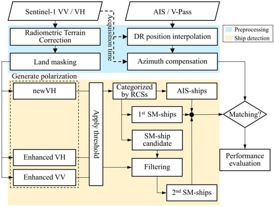
Figure 2.
Overall workflow for the ship detection and validation. Here, AIS = Automatic Identification System, V-Pass = Small Fishing Vessel Tracking System, DR = Dead Reckoning, RCS = Radar Cross Section, and SM-ships = Small-ships.
2.2.1. Pre-Processing
Radiometric Terrain Correction
Gamma software (version updated in December 2021), offering faster and more diverse SAR image optimizations than Sentinel Application Platform (SNAP) software (version 9.0.0) [35], was utilized for pre-processing, followed by obtaining a Digital Elevation Model (DEM) which matched the satellite image’s dimensions using the orbit file, performing calibration with the Look Up Table (LUT), and obtaining the final pre-processed image through geocoding combined with terrain correction.
Land Masking
The land masking procedure was accomplished using the Korea Hydrographic and Oceanographic Administration’s (KHOA) ENC-based land area map (LNDARE). By incorporating LNDARE-based coastline data and SAR satellite images, a dynamic land masking map generation method was proposed [36]. In this study, the land masking method was modified to correspond with Sentinel−1 SAR (Figure 3). Initially, image scaling based on histograms was used to improve land area detection, followed by finding the representative threshold value in the image corresponding to the LNDARE, and generating a potential land map. Then, the noise-removed land map was regenerated using canny edge detection, morphological functions, and median filtering, and converted into the polygon data format. Finally, these labeled polygon land data were compared with LNDARE, and if there was overlapping between the two datasets, the final land masking object was confirmed.
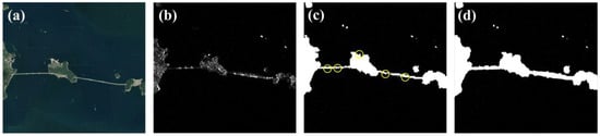
Figure 3.
Illustration of the land masking near Busan Newport. (a) Recent land area in a Google Earth image; (b) Land area in Sentinel−1 VH image; (c) Traditional land masking results with false detection (yellow circle); (d) Land masking results in this study after using the dynamic land masking method [33].
DR Position Interpolation
To compensate for the shortcomings of the AIS/V-Pass data caused by equipment failure [37], interpolation of the DR position was conducted [38]. The ship position, Speed Over Ground (SOG), and Course Over Ground (COG) before and after 30 min from Sentinel−1 acquisition time (SARt) were first extracted from the ship information. Subsequently, the ship data for AISt−1 and AISt+1 were obtained, which were closest to SARt, and the difference between the two times was computed as Δt = (SARt − AISt). However, if even one ship’s data do not exist within 30 min, then the DR position was calculated based on three cases. In the first case, the DR position was determined if only AISt−1 existed, and in the second case, the reverse DR position was determined if only AISt+1 existed. In the third case, the interpolated DR position was determined if both AISt−1 and AISt+1 were present. And then, SOG and COG were interpolated using Δt, respectively.
Azimuth Compensation
To address the Doppler effect [11,39,40], azimuth compensation was performed by using metadata from the Sentinel−1 image and ship information from AIS/V-Pass [41]. Sentinel−1 metadata were utilized to extract the azimuth direction (θsat), azimuth velocity (Vsat), and slant range (Rslant), while in situ data (AIS/V-Pass) were used to obtain the ship heading (θship) and ship velocity (Vship). Then, the direction of movement and the distance of movement were obtained using two formulas, which were required for azimuth shifting: firstly, radial velocity Rv = (Vship ∙ cos (θsat – θship + 2/π)), and secondly, azimuth ship distance δ = ((Rv/Vsat) ∙ Rslant). Then, Rv and δ were used to compute new coordinates that were moved from the original AIS and V-Pass coordinates, and azimuth compensation was completed.
2.2.2. Polarimetric Combination-Based Ship Detection (PCSD)
The ship detection technique proposed in this study has two distinctive features. First, rather than simply using the VV and VH polarizations provided by Sentinel−1, three distinct polarimetric images were generated and utilized. Among them, one polarized image was the combination of co- and cross-polarization, denoted as newVH. Second, independent polarimetric images were employed to reduce the false detection rate of SM-ships and AIS-ships. Algorithm 1 depicts the entire pseudocode for Polarimetric Combination-based Ship Detection (PCSD). In the first step, ship detection essentially involves comparing the target cells and training cells of CFAR and identifying pixels that surpass a specific threshold as targets. The mean and standard deviation were summed together to obtain the representative value of the training cell (AT). In the second step, three distinct forms of polarization were generated: newVH, enhanced VH, and enhanced VV. According to Ref. [21], newVH can eliminate Radio Frequency Interference (RFI) noise produced by VV, and is thus effective for detecting large ships. Furthermore, through real small-scale experiments, enhanced VH and enhanced VV were recognized as polarizations that can minimize noise [26,27]. However, this study adopted a modified threshold for small ship detection in Sentinel−1 image because the tested satellite platform and polarization are different from Sentinel−1. Step 3 included employing the newVH image to detect AIS-ships. To specifically detect AIS-ships, AT was applied only when the pixel value exceeded −10.36 (dB). Afterwards, SM-ships were detected by combining the results from newVH, enhanced VH, and enhanced VV polarization. The challenge with SM-ship detection was that the false detection rate increased when the SM-ship was identified as having a low RCS. SM-ship detection thus involved two different approaches. First, SM-ships were detected by adjusting the threshold to −16.98 (dB), which was the lowest possible level of false positives even in cases where SM-ships were detected correctly, and the results were denoted as first SM-ships. Secondly, distinct thresholds were utilized in enhanced VH and enhanced VV to detect different SM-ship positions since newVH alone generated a lot of noise when it was over −23.01 (dB). Afterwards, masking was performed, and the pixel location where the SM-ship detection candidates from three polarizations intersected was selected as the second SM-ships. Lastly, both the SM-ships detection results were combined to obtain the final SM-ship detection location.
| Algorithm 1: Ship detection method | |
| 1 | Input: , |
| Parameters (Target); Average of [x y] window size (Background); Standard deviation of [x y] window size , , , ; Threshold value for , , E, | |
| 2 | (Adaptive Threshold) |
| 3 | (newVH) |
| 4 | |
| 5 | |
| 6 | Function AIS-ships detection Obtain the data size of I: [Row, Col] ← size () p ← NVH (Row, Col) for pixel p ← 1 to I do if then ← Apply to Mask (, Land) Labeled ship object polygons from Derived centroid position from each polygon Output AIS-ships position |
| 7 | Function SM-ships detection Obtain the data size of I: [Row, Col] ← size () h ← (Row, Col) v ← (Row, Col) p ← NVH (Row, Col) for pixel h,v,p ← 1 to I do if then ← Apply to else if then ← Apply to ← Apply to ← Apply to ← merge () Mask (, ) then Mask (, ) then Mask (, ) then Mask (, Land) Labeled ship object polygons from Derived centroid position from each polygon Output AIS-ships and SM-ships position |
Two types of polarization images are provided by Sentinel−1: vertical waves transmitted and vertical waves received (VV polarization) and vertical waves transmitted and horizontal waves received (VH polarization). Depending on the polarization, different information can be obtained with varied features. For instance, a VH polarized image is considered to be better for detecting ships since wind-generated waves have less impact on the polarization [42,43]. However, human activities such as radio, mobile communication, television, and other satellites may result in RFI and azimuth smearing in SAR images (Figure 4a,c). To address this issue, Ref. [21] developed a new polarization technique called dual-pol, which was generated through the combination of VH and VV polarization and employed for ship detection. Using the methodology from previous research, newVH polarization was created in this study to suppress the azimuth smearing issue and RFI which result in the false positive detection of ships. Considering VH polarization as a base, which is effective for ship detection, this new polarization utilizes the adjusted VV polarization intensity values if the difference between the two polarizations is more than 6.53 (dB) (Algorithm 1: NVH). Figure 4b,d shows newVH images generated by combining the two polarizations that appear to successfully eliminate the azimuth smearing and RFI observed in Figure 4a,c.
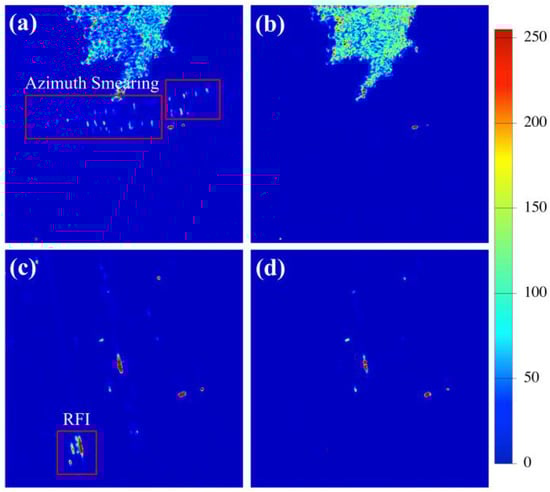
Figure 4.
Comparison between the Sentinel−1 VV and newVH pseudocolor images. (a,c) Display the VV polarization image; (b,d) Represent the same area in newVH polarization. Red rectangles indicate the noises caused by azimuth smearing and RFI (radio frequency interference) in VV polarization. For better visualization, the (dB) value was stretched from 0 to 255.
An illustration of AIS-ships detection utilizing AT (Algorithm 1) and the threshold value (Tat) with newVH as the input data is displayed in Figure 5. Among the two AIS-ships depicted in Figure 5e, the bottom ship measured 188 m in length and 30 m in width. The RCS (dB) in the Sentinel−1 image was measured to be as high as 28.27 (dB). The upper vessel, a general cargo ship, had a maximum RCS of −7.75 (dB) and measured 87 m in length and 30 m in width. These two ships masked the relevant pixel when a pixel with the criteria of being greater than −10.36 (dB) in newVH and having a threshold (Tat) of 25 or higher for AT met the requirements at the same time. Thus, it is apparent that only AIS-ships—aside from V-Pass—were detected (Figure 5e).
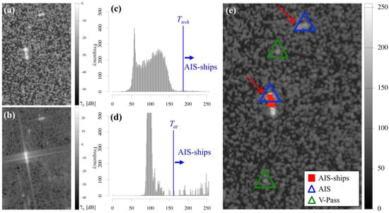
Figure 5.
Visualization of the approach for AIS-ships detection. (a,b) Display the ships in the Sentinel−1 VH and VV polarized image, respectively; (e) Shows the newVH image with the AIS-ship detection results (red rectangle pointed out with red arrow) along with the AIS (blue triangle) and V-Pass (green triangle) data; Histogram (c) represents the threshold value (Tnvh) applied in newVH; Histogram (d) represent the threshold value (Tat) from the AT. When both threshold conditions were satisfied the pixels were detected as AIS-ships (red rectangle) which also matched with the AIS (blue triangle) data. For a better understanding, the (dB) value was stretched from 0 to 255. Here, AIS = Automatic Identification System, and V-Pass = Small Fishing Vessel Tracking System.
Similar to the AIS-ships detection technique, the first step in the SM-ship detection process was performed with AT and Tat and the outcome was denoted as the first SM-ship. The threshold range for newVH and Tat was adjusted differently to detect the SM-ship, in contrast to the specifications for AIS-ships. While Tat was adjusted to be greater than 21, the threshold values for newVH ranged from greater than −16.98 (dB) to −10.36 (dB) or less. When both conditions were satisfied simultaneously, it was detected as an SM-ship using the identical approach. Figure 6 displays the threshold range of SM-ships and the detection result. After conducting the first step of the SM-ship detection method, three ships were detected (Figure 6b), and the ship on the upper side was concurrently identified as both an AIS-ship and an SM-ship. Therefore, the masking process was carried out for this ship to obtain only the SM-ships. As demonstrated in Figure 6c, the two ships that were successfully detected as ships had maximum RCS values that were −12.59 (dB) for the upper SM-ship and −12.37 (dB) for the bottom SM-ship. The first approach for detecting SM-ships searches for vessels with comparatively high RCS, regardless of their size, to avoid false positives from occurring beyond the detection target.
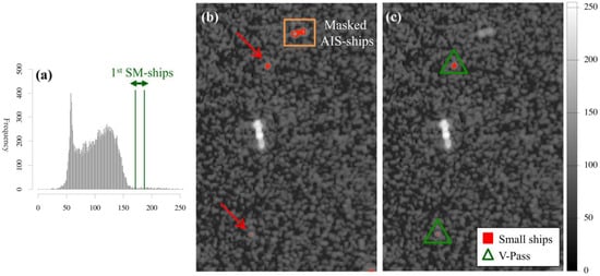
Figure 6.
Illustration of the first SM-ships detection phase from newVH image after the detection of AIS-ships (Figure 5). Histogram (a) represent the threshold range for the first SM-ships within the overall distribution of newVH; (b) displays the detection result (red rectangle pointed out with red arrow) after the thresholding operation; (c) represent the first SM-ships detection result (red rectangle) that matched with the V-Pass (green triangle) after removing the AIS-ships with amber rectangle in (b). For better understanding, the (dB) value was stretched from 0 to 255. Here, SM-ships = Small ships, AIS = Automatic Identification System, and V-Pass = Small Fishing Vessel Tracking System.
SM-ships with low RCS were the focus of the second stage of the SM-ship detection approach. However, false detections may increase as the target’s RCS lowers because speckle noise, which is simultaneously detected due to multiple factors like waves, can have an RCS similar to that of an SM-ship. As a result, rather than using a single polarization and method, we employed an approach that could reduce false positives by applying threshold values with different characteristics. Similar to the first SM-ship detection process, initially AT and Tat were employed, and the most suitable threshold parameters for the smallest ship were used in order to detect the candidate SM-ships. The threshold for newVH ranged from greater than −23.01 (dB) to −16.98 (dB) or less, while the Tat was greater than 7. However, within the threshold range, a considerable amount of noise also remained along with the candidate SM-ship targets. Therefore, to reduce these interferences, enhanced VH and enhanced VV—each with distinct characteristics—were applied for a second and third time. The SM-ships with low RCS were detected in the enhanced VH image by adjusting the threshold (Tevh) between −97.96 (dB) and −90.41 (dB). Similarly, the enhanced VV image’s threshold (Tevv) was set between −57.96 (dB) and −49.59 (dB). Although the threshold values of these two enhanced images were negative, the threshold values displayed here are rescaled from negative to 0 and maximum to 255.
Figure 7 illustrates the process of detecting a low RCS SM-ship, with an RCS as low as −22.01 (dB), in a Region of Interest (ROI) covering approximately 300 m 300 m, centered on the SM-ship’s location. Furthermore, the range of each threshold was stretched to visually depict the detection tendency of each polarization within an ROI characterized by a short spatial distance. In newVH, five clustered pixels were initially assembled, and the ship was detected (Figure 7k). Additionally, one noise was eliminated using Tat and AT. Through the enhanced VH ship identification results, one more noise was eliminated. At last, the last two noises were eliminated using enhanced VV, resulting in only a final few little ship pixels in the center (Figure 7n).
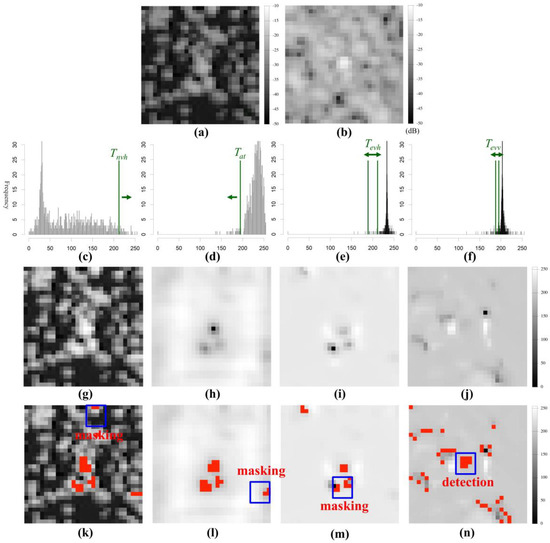
Figure 7.
Visualization of the second SM-ships (small ships) detection phase from the multiple polarization images within a region of interest (300 m 300 m). (a,b) Display the Sentinel−1 VH and VV images, respectively; Histogram (c) represent the threshold (Tnvh) within the newVH distribution, and (d) shows the threshold value (Tat) from the distribution of AT to detect the candidate SM-ships; Histogram (e) shows the range of threshold (Tevh) from enhanced VH, and (f) displays the threshold range (Tevv) of enhanced VV for detecting the SM-ships; (g–j) Represent the newVH, AT, enhanced VH, and enhanced VV after scaling the (dB) value from 0 to 255. (k–n) Show the detected pixels (red color) from each polarization images after the thresholding, respectively. The images display the step by step procedure of eliminating noise by using masking (blue rectangle), from the first detection (k) with 5 clustered pixels which form the newVH to the final clustered pixel detection (n). For a better understanding, the (dB) value was stretched from 0 to 255.
Contrary to Figure 7, Figure 8 shows an example of applying narrower minimum and maximum thresholds for each polarization in a larger ROI of 2 km 2 km. The threshold value that may detect the features of the SM-ship was biased more to one side in Figure 8c,d due to the large range of the ROI, and the threshold’s range was limited in Figure 8e,f. It can be observed that the four ship detection positions appeared differently when the threshold value was selected to be as similar as possible for SM-ships in each polarization. Since the characteristics of the images were diverse, it can be decided that false positives could be efficiently eliminated, as shown by each distribution graph.
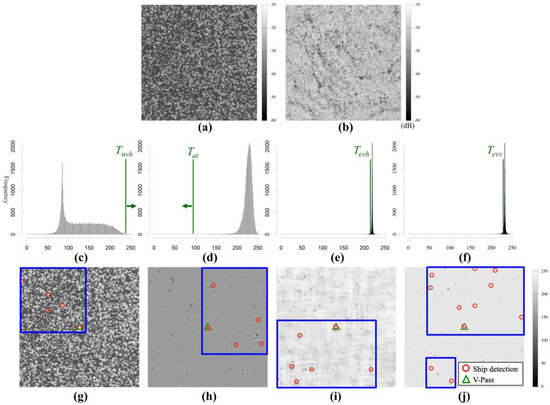
Figure 8.
Illustration of the second SM-ships detection phase from the multiple polarization images within a larger region of interest (2 km 2 km). (a,b) Show the Sentinel−1 VH and VV images, respectively; Histogram (c) represents the threshold (Tnvh) within the newVH distribution; Histogram (d) shows the threshold value (Tat) from the distribution of AT to detect the candidate SM-ships; Histogram (e) shows the range of threshold (Tevh) from enhanced VH; Histogram (f) displays the threshold range (Tevv) of enhanced VV for detecting the SM-ships. (g–j) Show the detected ship position (red circle) and detection area (blue rectangle) from the newVH, AT, enhanced VH, and enhanced VV, respectively, and the position was generated by centroid function using geometry coordinate of boundary from each clustered pixel, which was masked from polarization images after thresholding. The tendency of the detected position from each polarization images was different according to characteristic of polarization, and but one small ship at center point (green triangle) from V-Pass could be detected from all polarization. For a better understanding, the (dB) value was stretched from 0 to 255. Here, SM-ships = Small ships, and V-Pass = Small Fishing Vessel Tracking System.
2.2.3. Matching
This study’s methodology may cause false positives in the case of some large ships’ detection. Considering the bulk carrier’s design from the ship type information obtained by AIS, this ship structure has an elevated slope at only a specific location, such as bow anchor storage and the stern bridge. However, the middle location for bulk cargo storage has practically no inclination. Due to the ship’s structure, the bow and stern usually possess high RCS values, while the middle portion of the ship typically has low RCS values, resulting in it being detected as two small ships. To deal with this issue, this study proposed a technique to eliminate the probable false alarms. The first step was to cluster areas within 300 m of the previous vessel detection location to identify candidates for possible false alarms. After that, a ship chip image was created with the locations of each chosen candidate at its center. The ship chip image was binarized using an RCS threshold of 0.02, noise was eliminated using morphology operations, and the ship detection positions were reproduced based on the number of vectorized polygons. The maximum RCS value of SM-ships—obtained with the aid of V-Pass information—was used to establish the RCS standard.
The procedure for estimating a detected vessel’s length is referred to as ship discrimination, and the ship length determined in the following way was utilized to improve matching accuracy. The ship’s border for calculating ship length was established by applying sobel edge detection to the ship chip image. The detected ship’s position and length were compared to the ship’s position and length observed in AIS and V-Pass (Figure 9a). The ship was considered matched if the comparison results between the two observations met all of the requirements. However, as AIS was the only source of ship length information (Figure 9b), the discriminating procedure was limited to AIS, and V-Pass ships were matched to 20 m SM-ships.
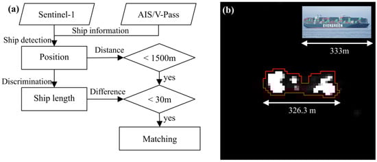
Figure 9.
Illustration of the ship discrimination approach for matching the detected ships with the ground truth. (a) Displays the workflow to discriminate the detected ship and match with the ground truth from AIS/V-Pass; (b) Shows a container ship detected from Sentinel−1 and discriminated based on the length (326.3 m) which matched with the ground truth length (333 m) obtained from the AIS. Here, AIS = Automatic Identification System, and V-Pass = Small Fishing Vessel Tracking System.
3. Results
In this section, the results of the detection of ships with the proposed method and their evaluation are depicted, where AIS and V-Pass were used as the validation data to evaluate the vessel detection results. The six evaluation items—AISmr, AISfr, SMmr, SMfr, AISMmr, and AISMfr—were used to assess the detection performance. AISmr (the matching ratio) is a coefficient that shows how successfully the AIS vessel was detected. The performance increases as it approaches 100. Then, AISfr (the false alarm ratio) indicates the number of false alarms that have happened, and the performance increases as it gets closer to 0. Similarly, the evaluation items SMmr and SMfr were used to display the small ship detection performance. Moreover, AISMmr and AISMfr are evaluation items that combine both AIS and V-Pass.
Furthermore, a comparative evaluation of the performance was conducted using the methodology of this study in conjunction with two representative previous ship detection studies. The first one was the Image Contrast Enhancement (ICE) method, which followed the approach proposed by Ref. [1] and considered the characteristics of the study area to improve ship detection performance for AIS-ships and reduce false positives as much as possible (Figure 10: ICE). The second approach used CFAR, and Ref. [21] employed an adaptive threshold for each detection target after dividing the detection target’s RCS into four levels to detect AIS-ships in the research area (Figure 10: ATM-CFAR). Figure 10 compares the locations of SM-ships using two ship detection methods, ICE and ATM-CFAR, applied to Sentinel−1 image captured on 6 April 2022. Examining the Busan Port anchorage sea area on the left side of the image, where AIS vessels were primarily located, it appears that vessel detection was successful using both methods. However, in the orange square area on the right side of the image (Figure 10), located in the open sea near Busan Port, it was observed that most SM-ships were not detected. In the research area, the AISmr’s performance in ICE-based vessel detection was 84.96% (113 ships detected out of 133 AIS ships), while the SMmr’s performance was only 10.53% (two ships detected out of nineteen V-Pass ships). Consequently, it can be concluded that detecting SM-ships was nearly impossible. On the other hand, ATM-CFAR exhibited a high AISmr performance at 91.73% (122 ships detected out of 133 AIS), and SMmr’s performance was 31.58% (six ships detected out nineteen 19 V-Pass ships), showing an improvement over ICE.
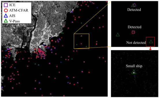
Figure 10.
Results of ship detection after applying the image contrast enhancement (ICE) and ATM-Constant false alarm rate (ATM-CFAR) approaches to scene no. 7 (6 April 2022). The detected positions of AIS-ships using ICE (purple rectangle) and ATM-CFAR (red circle) were highly matched with the AIS (blue triangle) while the V-Pass (green triangle) indicates that the small ships were not detected by these two methods. Here, AIS = Automatic Identification System, and V-Pass = Small Fishing Vessel Tracking System.
3.1. Test Result
The results of AIS-ship detection for scene no. 7 are displayed in Figure 11. There were 133 AIS ships total in that area, of which 152 AIS-ships were detected and 125 were matched. Hence, the calculated AISmr was 93.99%, and the calculated AISfr was 17.76%. The Busan Port ROI area’s detection results are displayed in Figure 11c. Reefer, tanker, general cargo, and other types of vessels were among those detected; the length of the vessels was determined to be between 57 and 126 m. Therefore, it can be verified that these ships were successfully detected.
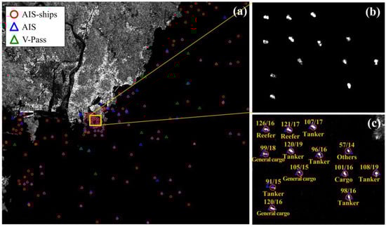
Figure 11.
Detection results for the AIS-ships (a) in scene no. 7 after applying the proposed method. (b) Display binarized image with 0 (black pixel) and 1 (white pixel) for the detected AIS-ships within the amber rectangle; (c) Shows the matching result of detected AIS-ships’ position (red circle) with the AIS (blue triangle) data; In addition, (c) represent the detail information on the ship type and length obtained from the AIS. Most of the V-Pass ships (green triangle) remain without matching (a). Here, AIS = Automatic Identification System, and V-Pass = Small Fishing Vessel Tracking System.
Figure 12 displays the results of the SM-ship detection using only newVH, and Figure 13 illustrates the findings of the SM-ship detection utilizing three polarization images concurrently. A total of 19 SM-ships were observed (V-Pass), 61 SM-ships were detected, and 12 SM-ships were matched. In the first step of detection, 57 SM-ships were detected, with nine matches and a detection rate of 15.79% (SM1mr). The RCS of the matched SM-ships ranged from −10.36 (dB) (S7) to −16.77 (dB) (S4). While the detection rate of the first step was low, visual confirmation revealed that other detected SM-ships that were not matched also corresponded to actual SM-ships. In the second step of detection, four SM-ships were detected, with three matches, resulting in an SM2mr of 75%. This indicates the accurate identification of low-RCS ships without false positives. The RCS of the matched SM-ships ranged from −19.50 (dB) (S10) to −22.01 (dB) (S12). Combining the results from both the first and second detections, the final SMmr was calculated to be 63.16%.
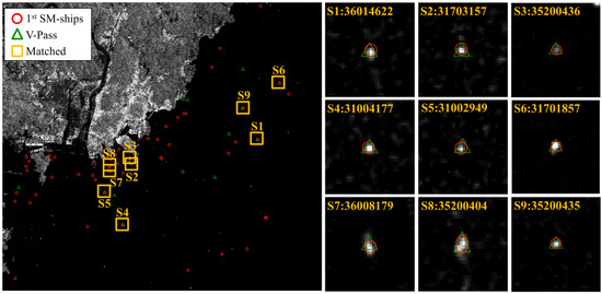
Figure 12.
Detection results for first small ships (SM-ships) in the newVH image (scene no. 7). Red circle indicates the detected position of first SM-ships, green triangle represents the V-Pass and amber rectangle display the matching results. The ID and shape of each matched image are displayed in the right. Here, V-Pass = Small Fishing Vessel Tracking System.
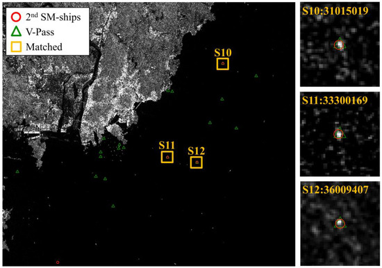
Figure 13.
Detection results for second small ships (SM-ships) in multiple polarization (scene no. 7). Red circle indicates the detected position of second SM-ships, green triangle represents the V-Pass and amber rectangle display the matching results. The ID and shape of each matched image are displayed in the right. Here, V-Pass = Small Fishing Vessel Tracking System.
The PCSD results from this study were compared with the detection results of the ICE and ATM-CFAR methods, which are recognized for their higher AIS-ship detection capabilities (Table 2). The AISmr exhibited either a higher or equivalent performance compared to ICE and ATM-CFAR. However, the AISfr of this method demonstrated a lower false positive rate compared to the other two methods. The results obtained from PCSD’s SMmr indicated a considerable improvement in SM-ship detection capability, exceeding the results of the other two methods by more than two times. When considering AISMmr and AISMfr, which represent the overall detection results combining AIS and V-Pass, they exhibited better performances than the ATM-CFAR model.
Table 2.
The performance of ship detection using three distinct vessel detection models in scene no. 7.
3.2. Model Comparison for Entire Dataset
Figure 14 displays the results of using the three models on 26 scenes acquired in 2022. However, scene number 10 was not included in the calculation of the detection rate and false detection rate since it only contained information about two vessels that was retrieved from AIS/V-Pass, causing uncertainties regarding the reliability of the information. Figure 14a depicts that the PCSD’s average AISmr was 86.67%, around 2% higher than the ATM-CFAR (84.92%). In addition, in the PCSD, the AISfr was 33.86%, and the false positive rate was over 10% lower than that of the ICE model (46.48%). Hence, PCSD was found to be more accurate for AIS-ship detection than the other two methods, with a higher detection rate and a lower false detection rate.
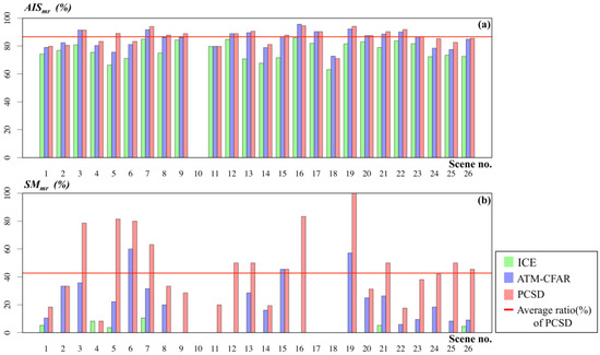
Figure 14.
Comparison graph illustrating the performance of three different ship detection models for the year 2022 (26 scenes). (a) Represents the matching ratio for AIS-ships; (b) Displays the matching ratio for the small ships. Here, AIS = Automatic Identification System, SM = Small ships, ICE = Image Contrast Enhancement, ATM-CFAR = ATM-Constant False Alarm Rate.
Figure 14b showed that, with an SMmr of 42.72%, PCSD achieved a detection rate twice as high as ATM-CFAR (18.53%), indicating that small ships surpassed AIS-ships in terms of detection rate. Furthermore, in scene 19, a detection rate of 100% was achieved with seven out of seven V-Pass ship detections, while scene 16 attained a detection rate of 83% with five out of six V-Pass vessel detections. These results revealed that a high performance can be achieved even with a small number of ships. Moreover, in scene 5, a detection performance of 81% was achieved with 22 detected ships out of 27 V-Pass ships, demonstrating a high performance even in scenarios with numerous ships. Additionally, there were 10 scenes with a final detection rate exceeding 50%. In addition, it can be assumed that the significant deviation observed in the overall detection rate might be attributed to the presence of certain small ships constructed from materials challenging to detect in the Sentinel−1 image or error’s occurred during V-Pass transmission.
To visualize and compare the different model’s performances, the Receiver Operator Characteristics (ROC) classification scheme was used. Generally, the ROC curve plots the True Positive Rate (TPR) on the Y-axis against the False Positive Rate (FPR) on the X-axis at various threshold settings. The Area Under the Curve (AUC) represents the size and quantitatively estimates the model’s performance [26]. In this study, the matching rate was used as a substitute for the TPR, while the false alarm rate was used as a substitute for the FPR. The AUC values calculated for AIS-ships using ICE, ATM-CFAR, and PCSD methods were 0.95, 0.96, and 0.95, respectively (Figure 15(a-1)–(a-3)). The results indicate that there was not a significant difference in performance among the three models, and performance was not dependent on the specific model used. In addition, a high performance is demonstrated with an AUC of 90 or higher. Moreover, Figure 15b illustrates an ROC graph calculated for SM-ships, demonstrating that the performance of PCSD (0.89) exceeds that of other models (0.76).
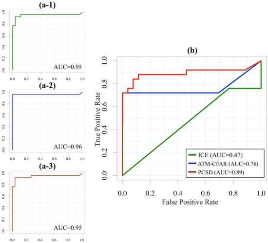
Figure 15.
Comparison of ship detection models: Receiver Operator Characteristics (ROC) curves for (a-1) ICE, (a-2) ATM-CFAR, (a-3) PCSD based on AIS-ships and (b) SM-ships. Here, AIS = Automatic Identification System, SM = Small ships, ICE = Image Contrast Enhancement, ATM-CFAR = ATM-Constant False Alarm Rate, PCSD = Polarimetric Combination-based Ship Detection.
Moreover, statistical tests were utilized to compare the performance of the three different models across the 26 scenes, using four performance indices (AISmr, AISfr, SMmr, SMfr). Therefore, the Mann–Whitney U-test and the Kruskal–Wallis H-test were used with the significant level of 0.05 [44,45]. In the Mann–Whitney U-test, the p-values for almost all indices were calculated to be less than 0.001, with the exception of the index comparing AISmr with ATM-CFAR and PCSD, which exceeded 0.05. In the Kruskal–Wallis H-test, all indices yielded values less than 0.05 (p-value), indicating their passing. Thus, no significant difference was found among the three models.
4. Discussion
4.1. Wave Height Distribution at Detected Ship Position
In SAR images, marine environmental factors such as eddies, internal waves, swells, and strong waves result in high scattering characteristics. Furthermore, since the scattering characteristics of SM-ships resemble those of waves, the performance of ship detection may be diminished during bad weather conditions [11]. In this study, the trend of the occurrence of waves within the study area was identified by analyzing speckle noise in the marine environment, particularly in Sentinel−1 images. Figure 16a displays the wave height across the study region along with the detected ship position. Moreover, Figure 16b–d illustrate graphs for wave height distribution and the number of detected ships for one year (2022).
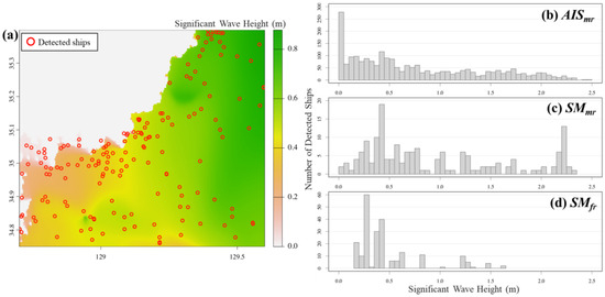
Figure 16.
Visualization of wave height across the study area. (a) Displays detected ships’ location (red circle) and significant wave height (m) for scene no. 7 (6 April 2022). (b–d) Depict the distribution of ship numbers corresponding to wave height, matched with AIS-ships, SM-ships, and false detection in SM-ships, respectively, for the year 2022. Here, AIS = Automatic Identification System, and SM = Small ships.
Firstly, it can be seen that AIS-ships were extensively distributed in areas of the sea characterized by low wave heights (Figure 16b). This phenomenon is attributed to the prevalence of large ships awaiting anchorage in regions where wave influence is minimal, which is consistent with the nature of the study’s sea area. Additionally, a significant number of SM-ships were detected at relatively low wave heights, with a decrease observed in the number of detected ships as the wave height approached or exceeded approximately 1 m. However, when the wave height exceeded 2 m, there was an increase in the number of detections for SM-ships (Figure 16c), although this phenomenon appears to be influenced by each backscattering characteristic of individual small ship or regional factors. Figure 16d depicts the distributions of SM-ships in areas where false detections occurred. Few false detections were observed at the high wave heights (>1 m), while the number of false detections was higher at low wave heights. Since the wave height data are modeled rather than measured, their reliability is not absolute. Therefore, analyzing wave effects should consider the scattering characteristics of individual ships and regional factors.
4.2. Comparison with DL Based Ship Detection
To identify dark fishing activity using SAR imagery, the Defense Innovation Unit (DIU) and Global Fishing Watch (GFW) have initiated an international competition. This competition employs modern machine learning (ML), deep learning (DL), and traditional computer vision approaches with the xView3-SAR dataset, comprising nearly 1000 analysis-ready SAR images from the Sentinel−1 satellite [46]. Among the proposed approaches, two DL models with high accuracy, DL-1: Selim_sef and DL-2: BloodAxe, were applied to the study region and then compared with PCSD (Figure 17). The DL models are accessible to everyone as open-source code (https://github.com/DIUx-xView, accessed on 3 March 2023), and they were installed using a Docker file. Geometric correction was subsequently applied to the results of the DL model to facilitate comparison. When a Sentinel−1 GRDH image is input, DL models provide candidate vessel detection locations and vessel/fishing status for each location. Then, these outputs could be compared with the AIS-ships and SM-ships detection results of this study.
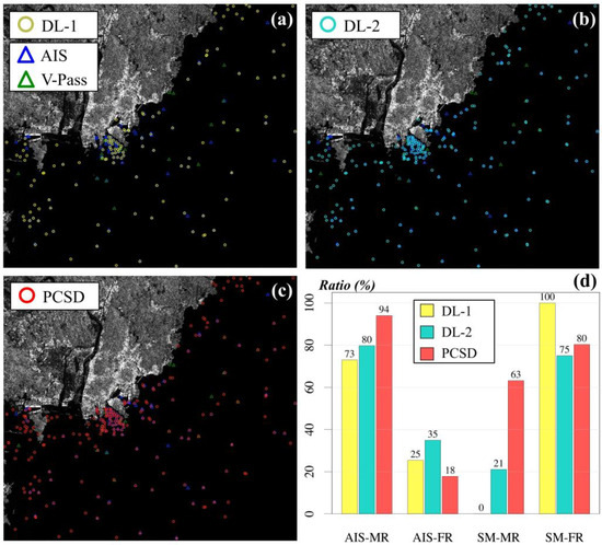
Figure 17.
Ship detection results and comparison graph using multiple DL model approaches for Scene no. 7 (6 April 2022). (a–c) Display the detected ships’ position using DL-1 (yellow circle), DL-2 (cyan circle) and PCSD (red circle) models, respectively, including AIS-ships and SM-ships. (d) Shows matching and false alarm ratio from AIS, and V-pass among the three different models. Here, DL = deep learning, AIS = Automatic Identification System, V-Pass = Small Fishing Vessel Tracking System, SM = Small ships, PCSD = Polarimetric Combination-based Ship Detection.
Figure 17 depicts the detection performance of the DL models and PCSD applied to scene no. 7. Considering the results of AISmr, the DL-1 and DL-2 models achieved accuracies of 72.93% and 79.70%, respectively, which were both significantly lower than ICE (84. 96%). Furthermore, the AISfrs of the DL-1 and DL-2 models were 25.38% and 34.90%, respectively. As a result, the detection performance of AISmr for the DL models was lower than that of the PCSD (17.76%), with a high number of false positives indicating poor overall detection performance for AIS-ships. In the case of SMmr, the DL-2 model detected only four out of nineteen V-pass ships, while the DL-1 model failed to detect any ships. Specifically, although two SM-ships were detected in the DL-1 model, neither of them matched V-pass, resulting in an SMfr of 100%. Conversely, the DL-2 model achieved a detection rate of 75% and performed relatively better in terms of SMfr compared to PCSD (80.33%). However, the detection performance itself is limited, as only four vessels out of nineteen were matched (sixteen detections).
In general, deep learning models are significantly influenced by the trends observed in the training dataset. The training datasets utilized for the deep learning models in this study were predominantly derived from European waters and the west coast of Africa. Therefore, an assumption can be made that the AIS vessels and their distinct characteristics observed in the study area will differ considerably. Additionally, V-Pass is a small-boat tracking system exclusively used in Korea, and it is anticipated to differ fundamentally from the fishing boat types identified in AIS. To ensure better performance using deep learning, it is believed that long-term data collection in the research area, the creation of a customized dataset, and the development of a tailored model will be required.
5. Conclusions
Ship detection employing SAR imagery has been widely considered as a major research topic in the field of maritime surveillance. However, speckle noise and other typical interferences in SAR data result in false ship detections. In particular, the detection of small vessels with low RCS exhibited a considerable potential for generating false-positive detections. Thus, to reduce false positives, we suggested an SM-ship detection approach in this study, and assessed the results after applying the method to 26 scenes. The conclusions of the study are as follows:
Two distinct strategies for ship detection were implemented by separating the AIS-ship threshold from the SM-ship threshold. Consequently, emphasis was given to enhancing the SM-ship detection performance while maintaining the high detection accuracy of the AIS-ships. For this purpose, three different polarizations—newVH, enhanced VH, and enhanced VV—were generated, and the SM-ship detection results from these polarizations were combined to remove the pixels that generate false positive alarms.
Utilizing ship data from AIS/V-Pass, the ship detection results were validated. To improve the ground truth’s reliability, ship information was updated through the DR interpolation and azimuth compensation approaches. By utilizing 26 scenes acquired in 2022, it was found that the average detection rate for AIS-ships was over 85%, and the detection rate for SM-ships was over 42%. Furthermore, the highest detection performance reached 100% in scene 19, with seven ships detected out of a total of seven V-Pass ships. In addition, a detection rate exceeding 50% was achieved in 10 scenes. Finally, the detection performance for AIS-ships remained consistent with that of other models designed for AIS, while the detection performance for SM-ships was improved by more than double compared to other models.
Author Contributions
Conceptualization, D.-W.S., C.-S.Y. and S.J.K.C.; methodology, D.-W.S., C.-S.Y. and S.J.K.C.; software, D.-W.S. and C.-S.Y.; validation, D.-W.S. and C.-S.Y.; formal analysis, D.-W.S. and C.-S.Y.; investigation, D.-W.S., C.-S.Y. and S.J.K.C.; resources, D.-W.S. and C.-S.Y.; data curation, D.-W.S.; writing—original draft preparation, D.-W.S. and S.J.K.C.; writing—review and editing, D.-W.S., C.-S.Y. and S.J.K.C.; visualization, D.-W.S. and C.-S.Y.; supervision, C.-S.Y.; project administration, C.-S.Y.; funding acquisition, C.-S.Y. All authors have read and agreed to the published version of the manuscript.
Funding
This research received no external funding.
Data Availability Statement
The Sentinel−1 images used in this study are openly available on the Copernicus Open Access Hub website (https://scihub.copernicus.eu/). The AIS/V-pass and environmental data will be made available on request.
Acknowledgments
This research work was supported by the projects ‘Remote Sensing Surveillance System for Supporting Illegal, Unreported and Unregulated (IUU) Fishing Control Activities’ funded by the Ministry of Foreign Affairs, Republic of Korea.
Conflicts of Interest
The authors declare no conflicts of interest.
References
- Jeong, J.; Yang, C.-S. Automatic image contrast enhancement for small ship detection and inspection using RADARSAT-2 Synthetic Aperture Radar data. Terr. Atmos. Ocean. Sci. 2016, 27, 463–472. [Google Scholar] [CrossRef][Green Version]
- Kang, M.; Ji, K.; Leng, X.; Lin, Z. Contextual region-based convolutional neural network with multilayer fusion for SAR ship detection. Remote Sens. 2017, 9, 860. [Google Scholar] [CrossRef]
- Nie, G.-H.; Zhang, P.; Niu, X.; Dou, Y.; Xia, F. Ship detection using transfer learned Single Shot Multi Box Detector. ITM Web Conf. 2017, 12, 01006. [Google Scholar] [CrossRef]
- Zhao, J.; Zhang, Z.; Yu, W.; Truong, T.-K. A cascade coupled convolutional neural network guided visual attention method for ship detection from SAR images. IEEE Access 2018, 6, 50693–50708. [Google Scholar] [CrossRef]
- Chang, Y.-L.; Anagaw, A.; Chang, L.; Wang, Y.C.; Hsiao, C.-Y.; Lee, W.-H. Ship detection based on YOLOv2 for SAR imagery. Remote Sens. 2019, 11, 786. [Google Scholar] [CrossRef]
- Gui, Y.; Li, X.; Xue, L.; Lv, J. A scale transfer convolution network for small ship detection in SAR images. In Proceedings of the 2019 IEEE 8th Joint International Information Technology and Artificial Intelligence Conference (ITAIC), Chongqing, China, 24–26 May 2019. [Google Scholar] [CrossRef]
- Wang, Y.; Wang, C.; Zhang, H.; Dong, Y.; Wei, S. A SAR dataset of ship detection for deep learning under complex backgrounds. Remote Sens. 2019, 11, 765. [Google Scholar] [CrossRef]
- Zhang, T.; Zhang, X.; Ke, X.; Zhan, X.; Shi, J.; Wei, S.; Pan, D.; Li, J.; Su, H.; Zhou, Y.; et al. LS-SSDD-v1.0: A deep learning dataset dedicated to small ship detection from large-scale Sentinel-1 SAR images. Remote Sens. 2020, 12, 2997. [Google Scholar] [CrossRef]
- Zhang, T.; Zhang, X.; Li, J.; Xu, X.; Wang, B.; Zhan, X.; Xu, Y.; Ke, X.; Zeng, T.; Su, H.; et al. SAR Ship Detection Dataset (SSDD): Official release and comprehensive data analysis. Remote Sens. 2021, 13, 3690. [Google Scholar] [CrossRef]
- Crisp, D.J. The State-of-the-Art in Ship Detection in Synthetic Aperture Radar Imagery; DSTO Information Sciences Laboratory: Edinberg, Australia, 2004. [Google Scholar]
- Jeon, H.-K. Faster SAR Ship Detection Based on Stepwise Threshold Method. Ph.D. Thesis, University of Science and Technology, Daejeon, Republic of Korea, August 2023. [Google Scholar]
- Kwon, S.J.; Shin, S.W. Study on the ship detection method using SAR imagery. J. Korean Soc. Geospat. Inf. Sci. 2009, 17, 131–139. [Google Scholar]
- Li, N.; Pan, X.; Yang, L.; Huang, Z.; Wu, Z.; Zheng, G. Adaptive CFAR method for SAR ship detection using intensity and texture feature fusion attention contrast mechanism. Sensors 2022, 22, 8116. [Google Scholar] [CrossRef]
- Chen, J.; Chen, Y.; Yang, J. Ship detection using polarization cross-entropy. IEEE Geosci. Remote Sens. 2009, 6, 723–727. [Google Scholar] [CrossRef]
- Brekke, C.; Anfinsen, S.N.; Larsen, Y. Subband extraction strategies in ship detection with the subaperture cross-correlation magnitude. IEEE Geosci. Remote Sens. 2013, 10, 786–790. [Google Scholar] [CrossRef]
- Yin, J.; Yang, J. Ship detection by using the M-Chi and M-Delta decompositions. In Proceedings of the 2014 IEEE Geoscience and Remote Sensing Symposium, Quebec City, QC, Canada, 13–18 July 2014. [Google Scholar] [CrossRef]
- Wang, W.; Ji, Y.; Lin, X. A novel fusion-based ship detection method from Pol-SAR images. Sensors 2015, 15, 25072–25089. [Google Scholar] [CrossRef] [PubMed]
- Zhang, J.; Xing, M.; Sun, G.-C.; Li, N. Oriented gaussian function-based box boundary-aware vectors for oriented ship detection in multiresolution SAR imagery. IEEE Trans. Geosci. Remote Sens. 2022, 60, 5211015. [Google Scholar] [CrossRef]
- Gao, G.; Yao, L.; Li, W.; Zhang, L.; Zhang, M. Onboard information fusion for multi satellite collaborative observation: Summary, challenges, and perspectives. IEEE Geosci. Remote Sens. Mag. 2023, 11, 40–59. [Google Scholar] [CrossRef]
- Wei, J.; Zhang, J.; Huang, G.; Zhao, Z. On the use of cross-correlation between volume scattering and helix scattering from polarimetric SAR data for the improvement of ship detection. Remote Sens. 2016, 8, 74. [Google Scholar] [CrossRef]
- Bae, J.; Yang, C.-S. A method to suppress false alarms of Sentinel-1 to improve ship detection. Korean J. Remote Sens. 2020, 36, 535–544. [Google Scholar] [CrossRef]
- Pelich, R.; Chini, M.; Hostache, R.; Matgen, P.; Lopez-Martinez, C.; Nuevo, M.; Ries, P.; Eiden, G. Large-scale automatic vessel monitoring based on dual-polarization Sentinel-1 and AIS data. Remote Sens. 2019, 11, 1078. [Google Scholar] [CrossRef]
- Hwang, S.I.; Ouchi, K. A new technique for the improved accuracy of small ship detection by Synthetic Aperture Radar imagery. In Proceedings of the 2009 International Symposium on Antennas and Propagation (ISAP 2009), Bangkok, Thailand, 20–23 October 2009. [Google Scholar]
- Liu, G.; Zhang, X.; Meng, J. A small ship target detection method based on polarimetric SAR. Remote Sens. 2019, 11, 2938. [Google Scholar] [CrossRef]
- Zhang, T.; Yang, Z.; Gan, H.; Xiang, D.; Zhu, S.; Yang, J. PolSAR ship detection using the joint polarimetric information. IEEE Trans. Geosci. Remote Sens. 2020, 58, 8225–8241. [Google Scholar] [CrossRef]
- Lanz, P.; Marino, A.; Brinkhoff, T.; Köster, F.; Möller, M. The InflateSAR campaign: Testing SAR vessel detection systems for refugee rubber inflatables. Remote Sens. 2021, 13, 1487. [Google Scholar] [CrossRef]
- Lanz, P.; Marino, A.; Simpson, M.D.; Brinkhoff, T.; Köster, F.; Möller, M. The InflateSAR campaign: Developing refugee vessel detection capabilities with polarimetric SAR. Remote Sens. 2023, 15, 2008. [Google Scholar] [CrossRef]
- Štepec, D.; Martinčič, T.; Skočaj, D. Automated System for Ship Detection from Medium Resolution Satellite Optical Imagery. In Proceedings of the OCEANS 2019 MTS/IEEE SEATTLE, Seattle, WA, USA, 27–31 October 2019. [Google Scholar] [CrossRef]
- Wang, Y.; Wang, C.; Zhang, H. Combining a Single Shot Multibox Detector with transfer learning for ship detection using Sentinel-1 SAR images. Remote Sens. Lett. 2018, 9, 780–788. [Google Scholar] [CrossRef]
- Jeon, H.-K.; Han, J.R. Random forest classifier-based ship type prediction with limited ship information of AIS and V-Pass. Korean J. Remote Sens. 2022, 38, 435–446. [Google Scholar] [CrossRef]
- Kim, T.-H.; Jeong, J.; Yang, C.-S. Construction and operation of AIS system on Socheongcho Ocean Research Station. J. Coast. Disaster Prev. 2016, 3, 74–80. [Google Scholar] [CrossRef]
- Jeong, J.; Kim, T.-H.; Yang, C.-S. Construction of real-time remote ship monitoring system using Ka-band payload of COMS. Korean J. Remote Sens. 2016, 32, 323–330. [Google Scholar] [CrossRef][Green Version]
- Shin, D.-W.; Yang, C.-S.; Harun-Al-Rashid, A. Prediction of longline fishing activity from V-Pass data using Hidden Markov model. Korean J. Remote Sens. 2022, 38, 73–82. [Google Scholar] [CrossRef]
- Lee, D.Y.; Park, K.S.; Shi, J. Establishment of an operational oceanographic system for regional seas around Korea. Ocean Polar Res. 2009, 31, 361–368. [Google Scholar] [CrossRef][Green Version]
- Navacchi, C.; Cao, S.; Bauer-Marschallinger, B.; Snoeij, P.; Small, D.; Wagner, W. Utilising Sentinel-1’s orbital stability for efficient pre-processing of radiometric terrain corrected gamma nought backscatter. Sensors 2023, 23, 6072. [Google Scholar] [CrossRef]
- Yang, C.-S.; Park, J.-H.; Rashid, A.H.-A. An improved method of land masking for Synthetic Aperture Radar-based ship detection. J. Navig. 2018, 71, 788–804. [Google Scholar] [CrossRef]
- Harati-Mokhtari, A.; Wall, A.; Brooks, P.; Wang, J. Automatic Identification System (AIS): Data reliability and human error implications. J. Navig. 2007, 60, 373–389. [Google Scholar] [CrossRef]
- Chaturvedi, S.K.; Yang, C.-S.; Ouchi, K.; Shanmugam, P. Ship recognition by integration of SAR and AIS. J. Navig. 2012, 65, 323–337. [Google Scholar] [CrossRef]
- Guide to Sentinel-1 Geocoding. Sentinel-1 Mission Performance Center. 2022. Available online: https://sentinel.esa.int/documents/247904/3976352/Guide-to-Sentinel-1-Geocoding.pdf/e0450150-b4e9-4b2d-9b32-dadf989d3bd3 (accessed on 25 November 2023).
- Song, J.; Kim, D.-J.; Kang, K.-M. Automated procurement of training data for machine learning algorithm on ship detection using AIS information. Remote Sens. 2020, 12, 1443. [Google Scholar] [CrossRef]
- Ouchi, K. Principles of Synthetic Aperture Radar for Remote Sensing; Tokyo Denki University Press: Tokyo, Japan, 2009. [Google Scholar]
- Vachon, P.W.; Wolfe, J. C-band cross-polarization wind speed retrieval. IEEE Geosci. Remote Sens. Lett. 2011, 8, 456–459. [Google Scholar] [CrossRef]
- Hannevik, T.N.A.; Eldhuset, K.; Olsen, R.B. Improving Ship Detection by Using Polarimetric Decompositions. FFI-Rapport 2015/01554. Available online: https://publications.ffi.no/en/item/improving-ship-detection-by-using-polarimetric-decompositions (accessed on 10 November 2023).
- Mann, H.B.; Whitney, D.R. On a test of whether one of two random variables is stochastically larger than the other. Ann. Math. Statist. 1947, 18, 50–60. [Google Scholar] [CrossRef]
- Kruskal, W.H.; Wallis, W.A. Use of ranks in one-criterion variance analysis. J. Am. Stat. Assoc. 1952, 47, 583–621. [Google Scholar] [CrossRef]
- Paolo, F.; Lin, T.T.T.; Gupta, R.; Goodman, B.; Patel, N.; Kuster, D.; Kroodsma, D.; Dunnmon, J. xView3-SAR: Detecting Dark Fishing Activity Using Synthetic Aperture Radar Imagery. Adv. Neural Inf. Process. Syst. 2022, 35, 37604–37616. [Google Scholar] [CrossRef]
Disclaimer/Publisher’s Note: The statements, opinions and data contained in all publications are solely those of the individual author(s) and contributor(s) and not of MDPI and/or the editor(s). MDPI and/or the editor(s) disclaim responsibility for any injury to people or property resulting from any ideas, methods, instructions or products referred to in the content. |
© 2024 by the authors. Licensee MDPI, Basel, Switzerland. This article is an open access article distributed under the terms and conditions of the Creative Commons Attribution (CC BY) license (https://creativecommons.org/licenses/by/4.0/).