1. Introduction
Remote sensing is a focal area of research that profoundly impacts various positive aspects of human life, including environmental monitoring, urban planning, and disaster management. Advancements in remote sensing technologies, particularly satellite imagery, have transformed our ability to observe and understand the Earth’s geographical features. However, the effectiveness of remote sensing applications often depends on the quality and consistency of satellite images, which can vary significantly across different spectral bands and sensors. Satellite images captured under different environmental conditions or with various sensors exhibit inherent feature variations, leading to domain differences [
1]. These variations are particularly noticeable across different multispectral bands, where each band captures specific wavelength ranges on the electromagnetic spectrum. Such domain variability constitutes significant challenges for machine learning and deep learning models in classification and semantic segmentation tasks. These models are sensitive to variations in the input data distribution, which can lead to decreased performance and generalizability [
2]. Deep learning methods utilized for the detailed analysis and interpretation of satellite images are particularly susceptible to performance degradation due to domain variability. For instance, a semantic segmentation model trained on satellite images from one spectral band or sensor configuration may underperform when applied to images from a different spectral band or sensor, even if the underlying geographical features and structures are similar [
3]. Similarly, models trained on satellite images from one spectral configuration may perform poorly for classification tasks when applied to data from a different spectral range, even if the essential geographical attributes remain the same [
4]. This issue manifests in the domain adaptation problem, which aims to adapt models to perform well across varying domains [
5,
6,
7,
8].
The recent literature has explored various approaches to tackle the domain adaptation challenge with generative adversarial networks (GANs), highlighting their growing significance as a tool in this area [
9,
10,
11]. In the field of remote sensing, the recent literature, including Benjdira et al. [
12] and Zhao et al. [
13], has reported the implementation of GANs to generate target domain images from source domain images, effectively bridging the gap between different domains and enhancing model performance on tasks like semantic segmentation. However, while many studies have concentrated on strengthening downstream tasks such as segmentation or classification, the essential initial step of generating high-quality satellite images across multispectral bands or color channels has yet to be sufficiently addressed.
Considering this, our present work takes a step back to emphasize the generation aspect, which has implications for domain adaptation, a concept illustrated in
Figure 1. The diagram is divided into two segments, separated by dotted lines. The upper segment conceptually explores the rationale behind generating satellite images across spectral bands. This exploration envisions future initiatives to harness this capability, potentially enhancing the adaptability and performance of deep learning models across various domains. This segment does not delve into specific deep learning tasks but rather serves as a conceptual reasoning of addressing domain variability challenges.
The lower segment of the figure directly addresses our primary objective, i.e., to generate a satellite image
in a target spectral band
B from an original image
in a source spectral band
A. For illustrative clarity, in
Figure 1,
P denotes a hypothetical deep learning model. Suppose
P is trained with a dataset from
to convert satellite images into expected images (Output 1). Considering that
and
share identical underlying structures and classes, ideally, feeding
into model
P should yield the same result as
. However, discrepancies in color or spectral composition may lead to divergent results (Output 2), as depicted by the red arrow in the figure. To prevent this divergence, the first step would be generating image
from
with a generative model. As shown in the figure, a generator
M integrated with an encoder–decoder architecture as shown in the figure can be trained on the source domain
to generate images corresponding to the target domain
. Upon successful training, selecting an image
to perform a deep learning task, for instance, allows the generation of
, mirroring the spectral band of
. The resultant image
can then be processed with model
P to achieve the desired outcome, as illustrated by yellow-colored arrows in the diagram.
Continuing, we propose a GAN architecture integrated with contrastive learning, specifically designed to generate realistic-looking satellite images across multispectral bands, motivated by the work of Han et al. [
14]. By focusing on generating high-quality, cross-domain satellite images, our approach addresses the inherent channel variability and lays a foundation for subsequent domain adaptation applications.
2. Related Work
Domain shift or variation has been an enduring problem in the remote sensing domain. Various models have identified and addressed several related issues, yet some aspects of domain variation still require further exploration and solutions. The domain variability problem in satellite images can be traced back to the work of Sharma et al. [
15] in 2014. Sharma et al. tackled the challenge of land cover classification in multitemporal remotely sensed images, mainly focusing on scenarios where labeled data are available only for the source domain. This situation is complicated by variability arising from atmospheric and ground reflectance differences. To address this, they employed an innovative approach using ant colony optimization [
16] for cross-domain cluster mapping. The target domain data is overclustered in their method and then strategically matched to source domain classes using algorithms inspired by ant movement behavior. In the same year, Yilun Liu and Xia Li developed a method to address a similar challenge of insufficient labeled data in land use classification due to domain variability in satellite images [
17]. Using the TrCbrBoost model, their approach harnessed old domain data and fuzzy case-based reasoning for effective classifier training in the target domain. This technique demonstrated significant improvement in classification accuracy, highlighting its effectiveness in overcoming the constraints of domain variability. Similarly, Banerjee and Chaudhuri addressed the problem of unsupervised domain adaptation in remote sensing [
18], focusing on classifying multitemporal remote sensing images with inherent data overlapping and variability in semantic class properties. They introduced a hierarchical subspace learning approach, organizing source domain samples in a binary tree and adapting target domain samples at different tree levels. The method proposed by Banerjee and Chaudhuri demonstrated enhanced cross-domain classification performance for remote sensing datasets, effectively managing the challenges of data overlapping and semantic variability [
18].
Building on previous advancements in domain adaptation to address domain variability for remote sensing, Postadjian et al.’s work addressed large-scale classification challenges in very high resolution (VHR) satellite images, considering issues such as intraclass variability, diachrony between surveys, and the emergence of new classes not included in predefined labels [
19]. Postadjian et al. [
19] utilized deep convolutional neural networks (DCNNs) and fine-tuning techniques to adapt to these complexities, effectively handling geographic, temporal, and semantic variations. Following the innovative approaches in domain adaptation to address domain variability, Hofman et al. uniquely applied the CycleGAN [
20] network technique to generate target domain images to bridge domain gaps [
21]. This approach, leveraging cycle-consistent adversarial networks, enhances the adaptability of deep convolutional neural networks across varied environmental conditions and sensor bands, facilitating effective domain adaptation in unsupervised adaptation tasks, such as classification and semantic segmentation of roads, effectively overcoming pixel-level and high-level domain shifts.
Building on the momentum in addressing domain variability with generative adversarial networks, Zhang et al.’s work addressed the challenge of adapting neural networks to classify multiband SAR images [
22]. This work by Zhang et al. [
22] integrated adversarial learning in their proposed MLADA method to align the features of images from different frequency bands in a shared latent space. This approach effectively bridged the gap between bands, demonstrating how adversarial learning can be strategically used to enhance the adaptability and accuracy of neural networks in multiband SAR image classification [
22]. Similarly, a methodology proposed by Benjdira et al. focused on improving the semantic segmentation of aerial images through domain adaptation [
12]. This work utilized a CycleGAN-inspired adversarial approach, similar to the method employed by Hofman et al. [
21]. However, the approach by Benjdira et al. is distinguished by integrating a U-Net model [
23] within the generator. This adaptation enables the generation of target domain images that more closely resemble those of the source domain, effectively reducing domain shift related to sensor variation and image quality. Their approach demonstrated substantial improvement in segmentation accuracy across different domains, underscoring the potential of GANs to address domain adaptation challenges in aerial imagery segmentation. Along with this, to address a similar kind of domain variability, Tasar et al. introduced an innovative data augmentation approach, SemI2I, that employed generative adversarial networks to transfer the style of test data to training data, utilizing adaptive instance normalization and adversarial losses for style transfer [
24]. The approach, highlighted by its ability to generate semantically consistent target domain images, has outperformed existing domain adaptation methods, paving the way for more accurate and robust segmentation models with the generative adversarial mechanism in varied remote sensing environments.
Expanding on the work to address domain variability in remote sensing, another work by Tasar et al. [
25] effectively harnessed the power of GANs to mitigate the multispectral band shifts between satellite images from different geographic locations. Through ColorMapGANs, this work adeptly generated training images that were semantically consistent with original images yet spectrally adapted to resemble the test domain, substantially enhancing the segmentation accuracy. This intelligent use of GANs demonstrates their growing significance in addressing complex domain adaptation challenges in the remote sensing field. Consequently, Zhao et al. introduced an advanced method to minimize the pixel-level domain gap in remote sensing [
13]. The ResiDualGAN framework incorporates a resizing module and residual connections into DualGAN [
26] to address scale discrepancies and stabilize the training process effectively. Demonstrating its efficacy, the authors showcased significant improvements in segmentation accuracy on datasets collected from the cities of Potsdam and Vaihingen, open-source remote sensing semantic segmentation datasets [
27], proving that their approach robustly handles the domain variability and improves cross-domain semantic segmentation with a generative adversarial model. In the current literature on remote sensing, GANs and image-to-image translation mechanisms [
20,
26,
28,
29] have been promising in solving the domain variation problem. Since the translation of images from the source domain to the target domain is one of the fundamental building blocks in solving the domain variability problem, we present a GAN model inspired by the work of Han et al. [
14]. Han et al. presented an interesting approach for mapping two domains using generators within a GAN model, uniquely employing an unpaired fashion without a cyclic procedure. This approach demonstrates that reverse mapping between domains can be learned without relying on the generated images, leading to nonrestrictive mapping, in contrast to the restrictive mapping approach presented by Zhu et al. [
20]. Expanding on nonrestrictive mapping, our model integrates contrastive learning in a GAN with two generators and aims to perform better than well-established GAN models by generating realistic satellite images from one multispectral band to another. This capability is applicable for image generation and potentially beneficial for domain adaptation tasks.
3. Materials and Methods
This study aims to generate satellite images from one multispectral band mode to another, a process that can potentially help in domain adaptation within remote sensing. For this purpose, we conducted a thorough review of available datasets and selected an open-source dataset available from the ISPRS 2D Open-Source benchmark [
27], which has been frequently utilized in recent domain adaptation research [
12,
13]. This collected dataset includes different multispectral bands. For our analysis, we focused on two subsets: one from Potsdam City, with a pixel resolution of 5 cm and comprising the RGB (red, green, blue) spectral bands, and another from Vaihingen City, characterized by a 9 cm pixel resolution and including the IRRG (infrared, red, green) bands.
We consider two domains of satellite images,
and
, where the underlying features of an image
and an image
vary based on different multispectral bands. This scenario is formalized as the input domain
and the target domain
, where
and
represent the number of channels in each domain, respectively. Given sets of unpaired satellite images from these domains, we aim to generate a new image
from an input image
in domain
, such that
closely follows the true data distribution of domain
. We aim to accomplish this by constructing two mapping functions,
and
, such that
:
and
:
, where
S denotes a set of satellite images from the respective input domains. In this study, these two mapping functions,
and
, are demonstrated as two generators, to which there are two corresponding discriminators,
and
, as shown in
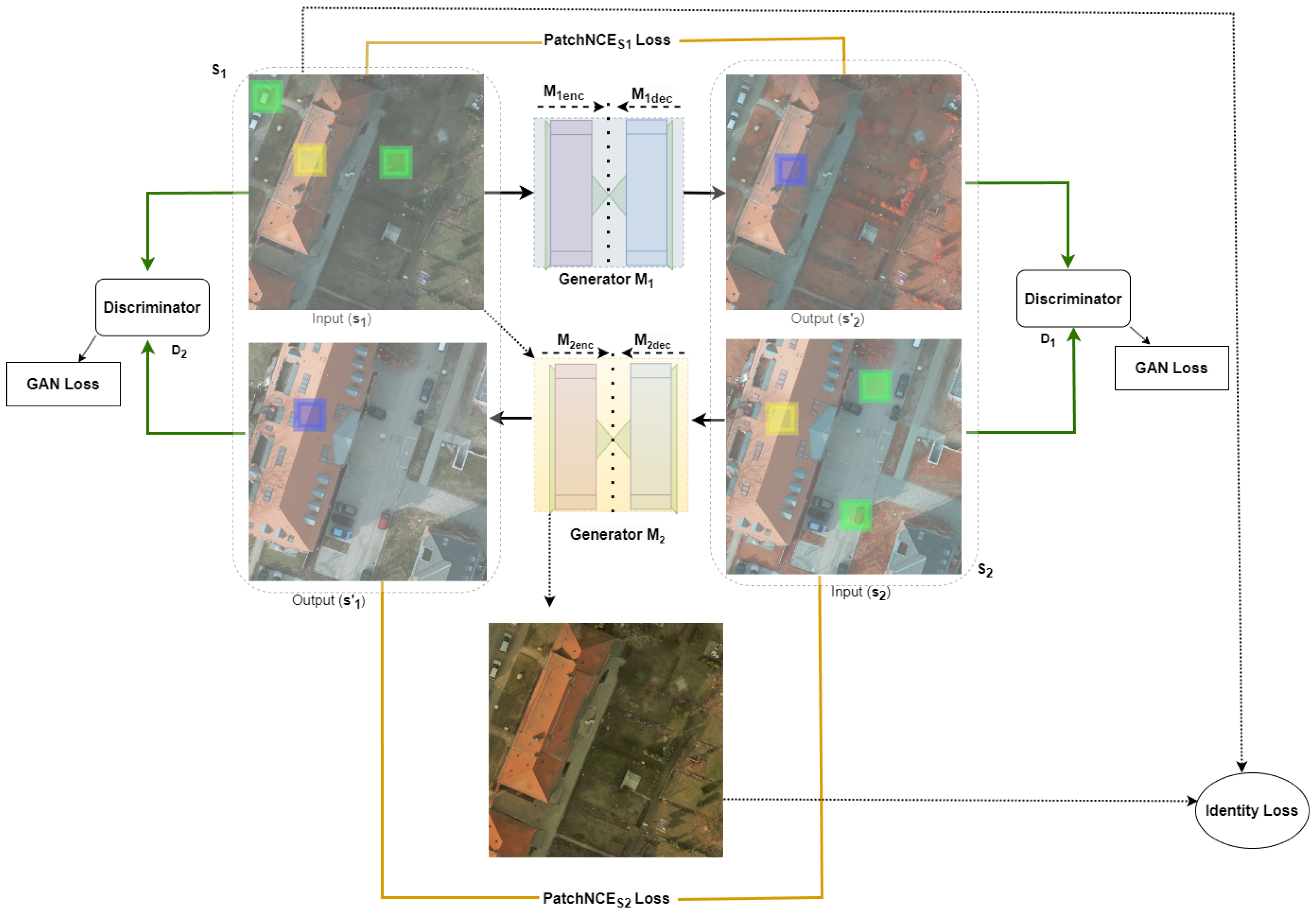
Figure 2.
3.1. Efficient Mapping with Generators
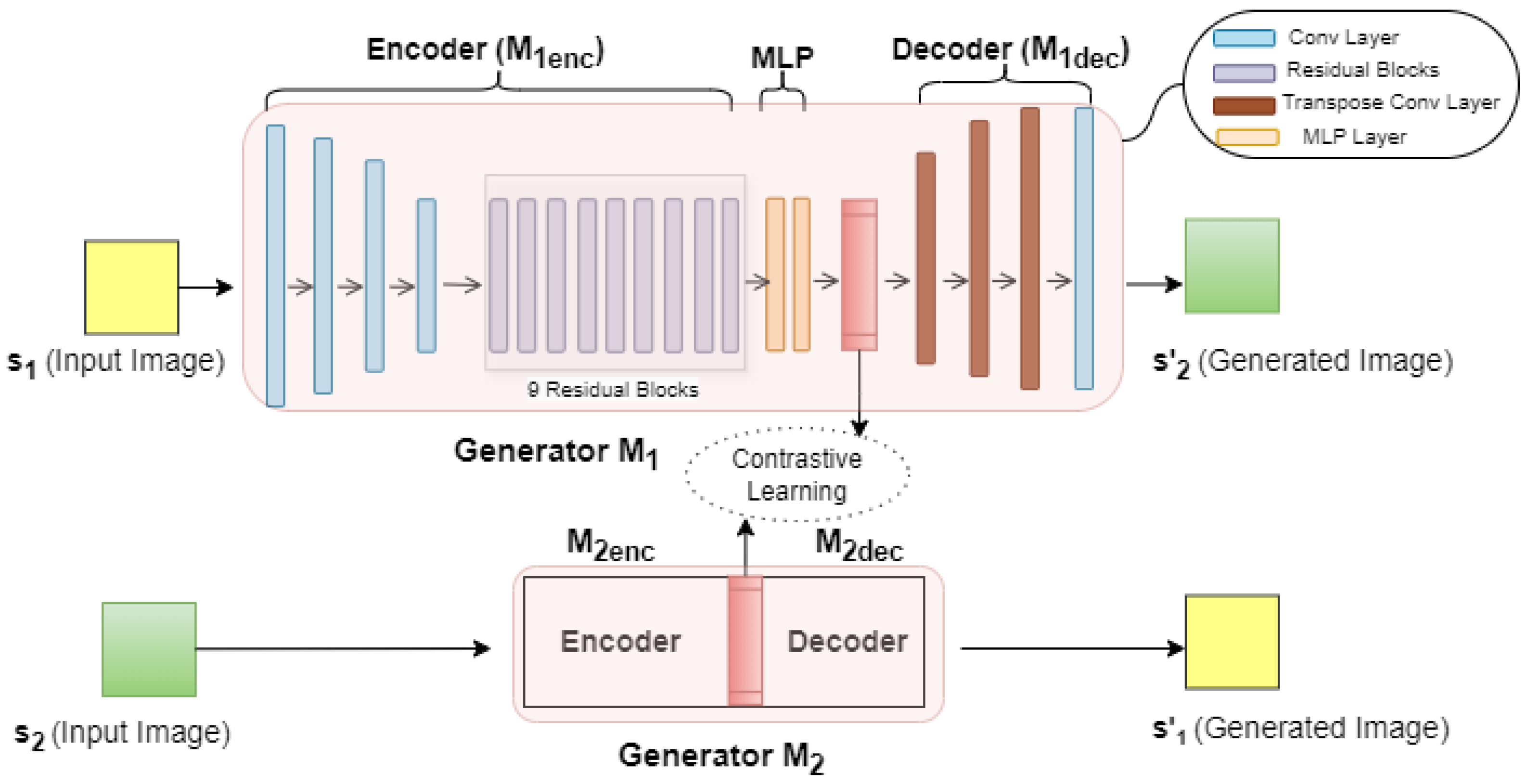
In the present work, each generator comprises an encoder-decoder architecture (as shown in
Figure 3), drawing inspiration from CUT [
28] and DCLGAN [
14] to generate designated satellite images. For each mapping and to better utilize the features in satellite images, we extract features from
encoder layers and propagate them to a two-layer MLP network (
and
), as performed in SimCLR [
30].
3.1.1. ResNet-Based Generator
The generators employed in this work are based on a ResNet architecture, as depicted in
Figure 3, which has been proven successful in various generative models [
31]. This choice is integral for synthesizing satellite images within our generative adversarial network (GAN) framework. The generator is designed to capture and translate the complex spatial and textural information in satellite images into corresponding images of different multispectral band representations. Motivated by [
20], each generator integrates nine residual blocks to help the encoding and decoding processes. These blocks enable the model to handle complex features essential for high-quality satellite images.
3.1.2. Encoder and Decoder Architecture
Building upon the initial framework, where the two mapping functions are represented as generators and , to which two corresponding discriminators, and , are assigned, we delve deeper into the architecture of these generators. Each generator consists of an encoder and a decoder component. The encoders, and , are used to capture and compress the spectral features of the satellite images from their respective domains. This is achieved by extracting features from layers of the encoder, as previously mentioned, which are then propagated to a two-layer MLP network to enhance feature utilization and facilitate effective domain translation.
The decoders,
and
(illustrated in
Figure 3), are responsible for reconstructing the image in the new domain while preserving spatial coherence and relevant features. They take the encoded features and, through a series of transformations, generate the output image that corresponds to the target domain. This process ensures that the translated images maintain the target domain’s essential characteristics while reflecting the source domain’s content.
With this procedure, the encoder and decoder collaborate within each generator to facilitate a robust and efficient translation between the multispectral bands of satellite images.
3.2. Discriminator Architecture
Discriminators are crucial for the adversarial training mechanism within the GAN framework. Our model incorporates two discriminators, and , each corresponding to generators, and , respectively. These discriminators distinguish between authentic satellite images and those synthesized by their respective generators. Their primary role is to provide critical feedback to the generators, driving them to produce more accurate and realistic translations of satellite images.
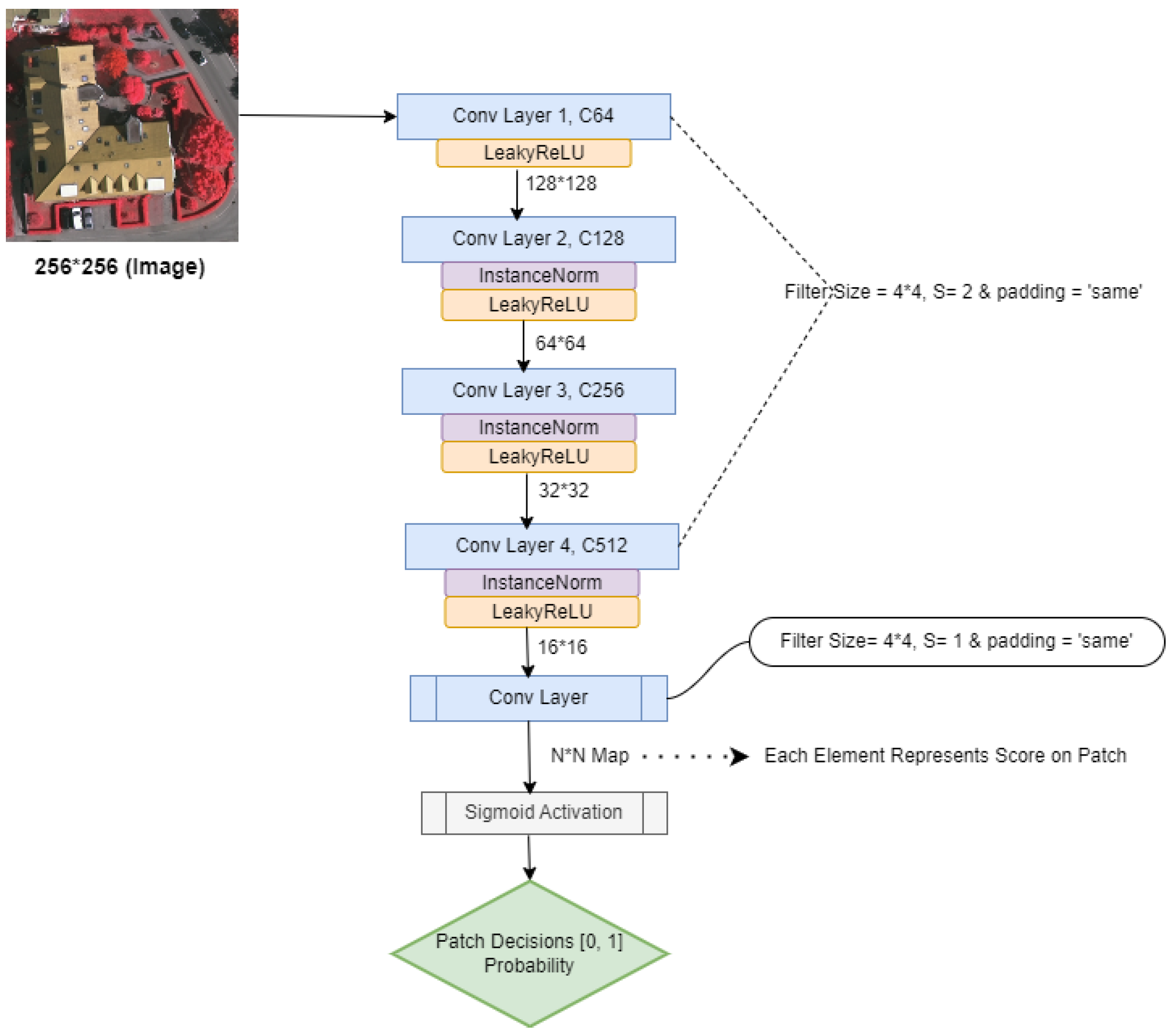
Our architecture employs a PatchGAN [
32] discriminator, chosen for its effectiveness in generative tasks. The architecture of the discriminator is depicted in
Figure 4. Unlike traditional discriminators that assess the authenticity of an entire image, PatchGAN divides the image into smaller
patches and evaluates the realism of each patch individually. The size of each patch,
p, is selected to be less than or equal to the height
H of the image, ensuring that each patch is reasonably sized to maintain a balance between training efficiency and feature learning. All the patches are processed through various convolution layers (depicted with blue-colored rectangles in
Figure 4, with deeper layers having an increasing number of filters. These convolution layers build up to a final convolution layer that assigns scores, indicating whether each patch is real or fake. The scores assigned to all patches by the discriminator are then aggregated to determine the overall authenticity of the image. This approach guides the generator in refining its output and facilitates the production of high-quality, realistic textures and patterns at the patch level.
Furthermore, we utilize instance normalization over batch normalization, as illustrated with purple-colored rounded rectangles in the diagram, a decision aligned with the best practices in image-to-image translation tasks [
20,
26,
28]. The integration of instance normalization contributes to the stability and performance of the model, particularly in the context of diverse and variable satellite imagery.
3.3. Contrastive Learning in the Present Work
Recently, contrastive learning has significantly advanced unsupervised learning in image processing, often outperforming conventional methods in scenarios with limited data [
30,
33]. It identifies negative and positive pairs and maximizes the mutual information relevant to the target objective.
3.3.1. Mutual Information Maximization
In our satellite image translation task, we devise an efficient method to maximize the mutual correlation between corresponding segments of the input and generated images across different multispectral bands. Specifically, a patch representing a particular land feature in the input image from domain
should be strongly associated with the corresponding element in the generated image in domain
, as shown in
Figure 2, where images
and
display the same building roof structure, highlighted with yellow and blue square patches, respectively. This approach ensures that relevant geographical and textural information is preserved and accurately represented in the translated images.
In the general procedure of the contrastive learning mechanism, we strategically select an anchor feature
, extracted from
(as shown in
Figure 2, highlighted with a blue-colored square), and a corresponding positive feature
, extracted from
(as shown in
Figure 2, depicted with a yellow-colored square), where
K represents the feature space dimensionality. Additionally, we sample a set of negative features
, with each
, from
. These negative features are drawn from different locations within the same image from which the corresponding
p was specified (depicted with green-colored squares in
Figure 2). All these features are represented as vectors and normalized with
-normalization [
34]. Subsequently, we construct an
-way classification task. In this task, the model evaluates the similarity between an anchor and various positive or negative elements. We direct the model to adjust the scale of these similarities using a temperature parameter,
= 0.07, before converting them into probabilities [
28]. This temperature scaling fine-tunes the model’s confidence in its predictions, facilitating a more effective learning process through the contrastive mechanism. After establishing this setup for normalization and predictions, we compute the probability that the positive element is more aligned to the anchor than any negative element. This probability is obtained using a cross-entropy loss, expressed mathematically as
where
denotes the cosine similarity between
a and
p, calculated as
[
30]. Through this loss equation, we effectively maximize the mutual correlation between matching segments, ensuring that the translation between multispectral bands of satellite images retains high fidelity and relevance.
3.3.2. PatchNCE Loss Mapping of Two Domains of Satellite Images
Utilizing the encoders and from the generators and , we extract features from the satellite images in domains and , respectively. For each domain, features are extracted from selected layers of the respective encoder and then propagated through a two-layer MLP network. This process results in a stack of feature layers , where each represents the output of the l-th selected layer after processing through the MLP network. Specifically, for an input image from domain , the feature stack can be represented as , where denotes the output of the l-th layer of encoder , and represents the corresponding MLP processing for that layer. Similarly, for domain , the feature stack is obtained using encoder and its corresponding MLP layers, which is given by , where is a generated image.
Our framework defines spatial locations within a layer to refer to distinct areas in the generated feature maps. Each spatial location is associated with a specific region of the input image, as determined by the network’s convolutional operations. We denote the layers by and the spatial locations within these layers by , where represents the total number of spatial locations in layer l. We then define an anchor patch and its corresponding positive feature as and all other features (the “negatives”) as , where denotes the number of feature channels in each layer, and Y represents the conceptual set containing all possible indices of these spatial locations within a layer.
By obtaining insights from CUT [
28] and DCLGAN [
14], the present work incorporates patch-based PatchNCE loss that aims to align analogous patches of input and output satellite images across multiple layers. For the mapping
, the PatchNCE loss is expressed as
Similarly, for the reverse mapping
, we utilized similar PatchNCE loss:
Through these formulations, the PatchNCE losses effectively encourage the model to learn translations that maintain the essential characteristics and patterns of the geographic features in satellite images, ensuring that the translated images retain the contextual and spectral integrity necessary for accurate interpretation and analysis.
3.4. Adversarial Loss
The present work utilizes an adversarial loss function to ensure the generation of realistic-looking satellite images from one domain to another based on different multispectral bands [
35]. The objective is to maintain balanced training of the generator and the discriminator to produce satellite images in the target domain that are indistinguishable from ground-truth satellite images. The discriminator learns to differentiate between the original and synthetic satellite images. The training is guided by the adversarial loss function with backpropagation and iterative updates of the layers’ weights in the model. Each generator,
and
, has a corresponding discriminator,
and
, respectively, ensuring a targeted adversarial relationship. The GAN loss for each generator–discriminator pair can be formulated as
In these equations,
and
represent the discriminator’s decision for ground-truth satellite images,
and
, respectively.
and
are the images generated from the input satellite images
and
that should hypothetically correspond to
and
, respectively. Real satellite images form
and
distributions from each domain. The generators
and
aim to minimize these losses, while the discriminators
and
aim to maximize them [
35]. Hence, the given loss function is termed adversarial, as the given generator and discriminator compete to get better and produce visually promising satellite images.
3.5. Identity Loss
Identity loss with mean squared error (MSE) is implemented to preserve the essential characteristics of the input image when it already belongs to the target domain. This approach ensures the generator minimizes alterations when the input image exhibits the target domain’s characteristics. Specifically, in our satellite image translation task, when generator is trained to convert an image from domain to an equivalent image in domain , it should ideally introduce minimal changes if an image from is provided as input. This strategy encourages the generator to maintain the identity of the input when it aligns with the target domain.
Mathematically, the identity loss for generator
when an image from
is fed as input using MSE can be expressed as
where
denotes the squared L2 norm, representing the sum of the squared differences between the generated and input images. A similar identity loss is applied for generator
when an image from
is fed:
Total identity loss, combining the contributions from both generators, is given as
Although we experimented with identity loss using the L1 norm, i.e., mean absolute error (MAE), we found that the L2 norm provided better results in our model. Therefore, we chose to utilize the L2 norm for identity loss. In practice, identity loss aids in stabilizing the training of the generators by ensuring they do not introduce unnecessary changes to images that already possess the desired characteristics of the target domain. This concept, inspired by the work of Zhu et al. [
20], is particularly beneficial in maintaining the structural and spectral integrity of satellite images during the translation process.
3.6. Final Objective
Our satellite image generation framework is depicted in
Figure 2. In our framework, the objective is to generate images that are not only realistic but also maintain a correspondence between patches in the input and output images. To achieve our goal, we integrate the combination of the GAN loss, PatchNCE loss, and identity loss to have our final loss function, which is given as
5. Discussion
In selecting datasets available from [
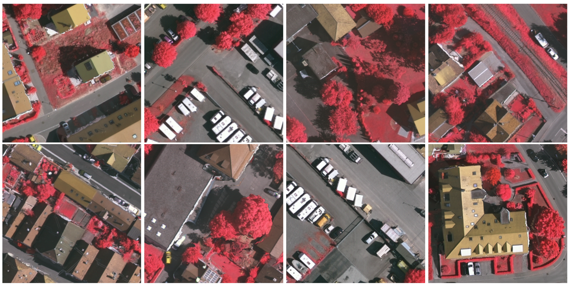
27], our goal was to generate satellite images with IRRG color composition similar to those collected from Vaihingen City (example images are shown in
Figure 7) by training the model on satellite images with RGB color composition collected from Potsdam City (images are shown in
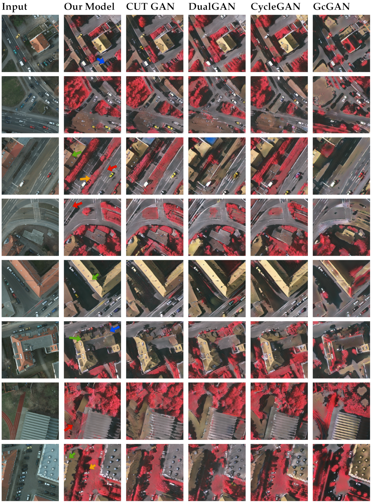
Figure 5 in the first column, i.e., Input). These two datasets generally have similar underlying features, such as buildings and roads, but the images in the input and target domains do not have one-to-one correspondence as they are taken from two different locations. During this, our training approach yielded promising results in image generation, as demonstrated in
Figure 5.
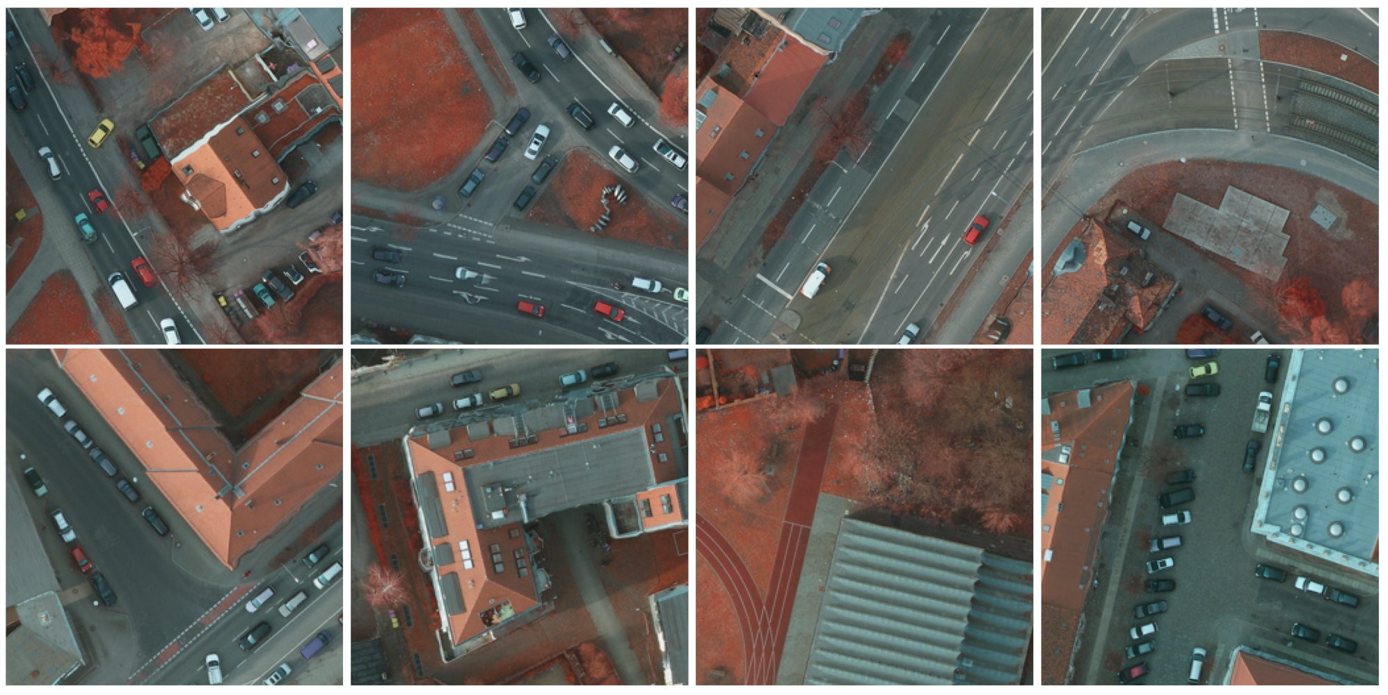
For the evaluation metrics SSIM, PSNR, and RMSE, it is generally necessary to have the exact generated image corresponding to the input image and the exact ground-truth image for the input image. Since the Potsdam and Vaihingen datasets are collected from two different cities, if the input image
A is from Potsdam and the target image
B is from Vaihingen, the ground truth image should maintain the underlying structure of
A but adopt the color composition of
B to align with our work of transferring between two different multispectral bands. The Potsdam dataset provides corresponding IRRG images for each RGB image; hence, during the calculation of SSIM, PSNR, and RMSE, we used related Potsdam IRRG color composition images (as shown in
Figure 8) as ground truth for each corresponding generated image.
Similarly, as observed in
Figure 5, the generated images exhibit a color composition similar to the target dataset, i.e., IRRG color composition satellite images from Vaihingen City, as shown in
Figure 7, aligning with our primary objective of replicating the target spectral characteristics. The presence of diverse objects such as buildings, cars, houses, and roads complicates the clear differentiation between the successes and failures of our model, especially in focusing on specific details. Upon detailed examination, we identified certain areas where our model outperforms or falls short compared to other models, as indicated by arrows in various colors. Specifically, as seen in
Figure 5 in rows 3, 5, 6, and 8, our model exhibits marginally better performance in preserving the structural details of certain parts of the roofs on houses and buildings, depicted with green-colored arrows. Furthermore, our model more effectively retains white-colored road markings, another underlying structure, as indicated by red-colored arrows in rows 3, 4, and 7. Additionally, in rows 1 and 6, our model effectively prevents inappropriate color generation, such as on cars and roofs, as highlighted by blue-colored arrows. Although these improvements are subtle, they underline the model’s enhanced capability to prevent inaccurate color generation.
There are, however, some deficiencies in our model, such as the incorrect generation of red color on roads, particularly in row 3, as indicated by a yellow-colored arrow. It is worth mentioning that all comparative models exhibit this same misrepresentation, suggesting that the flaw may be attributed to an imbalance in the dataset. Similarly, our model incorrectly merges black-colored cars with shadows, as depicted by yellow-colored arrows in row 8, a problem also common among the other models. This issue may be attributed to either dataset imbalance or the presence of shadows in the input images. Again, the same observation can be seen with all other models, showing the same performance of blending those cars into the shadow. This failure may also be attributable to the imbalanced dataset or shadows in the input images. An interesting observation was made on GcGAN [
29] regarding the retainment of specific structures. Despite inaccurately generating red color on roofs of buildings and houses, it successfully retained white-colored road markings similar to our results, where other models failed.
6. Conclusions
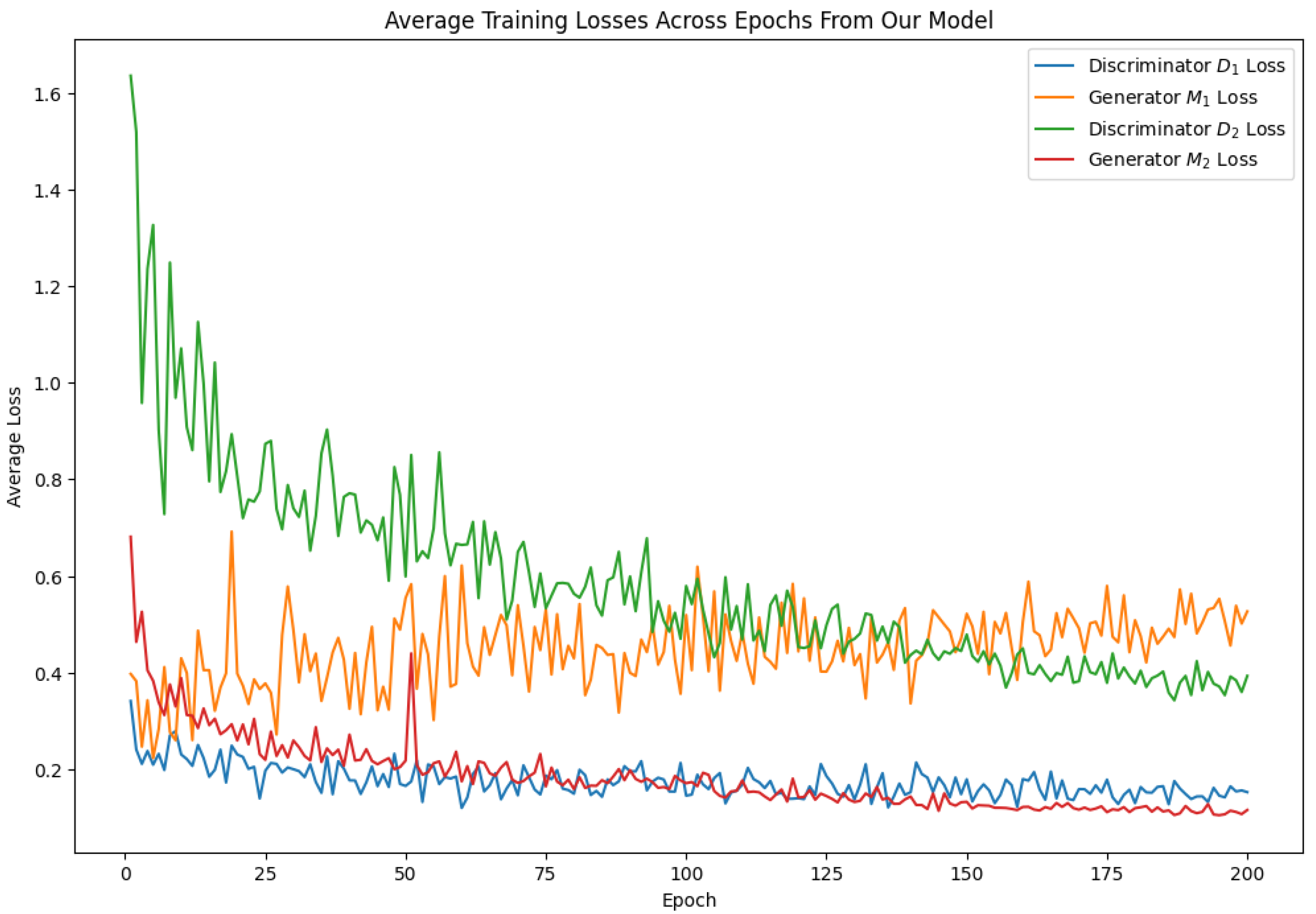
Satellite imagery, characterized by its diverse spectral bands, inherently exhibits domain variability that significantly impacts the performance of various analytical models. In response to this challenge, our work introduced an approach that leverages the capabilities of generative adversarial networks (GANs) combined with contrastive learning. Specifically, the present work incorporates a dual translating strategy, ensuring that each translation direction uses original images from the respective domains ( and ) rather than relying on previously generated images, maintaining the integrity and quality of the translation process. Our model effectively translates images across multispectral bands by integrating adversarial mechanisms between generators and discriminators, maximizing mutual information among important patches and utilizing identity loss with mean squared error (MSE). The quantitative results, as evidenced by metrics such as SSIM, PSNR, and RMSE, alongside qualitative visualization, demonstrate that our model performs better than well-established methods, including CycleGAN, CUT, DualGAN, and GcGAN. Furthermore, for training over 200 epochs, our model requires a comparable amount of time, around eleven hours, similar to that of the other models except for GcGAN, which took only nine hours to train but obtained a significantly lower SSIM value of 0.5786 compared to our model’s 0.7888. These findings highlight the practicability of our model in generating high-quality satellite images. These images accurately reflect the desired spectral characteristics while retaining important underlying structures, highlighting advancements in remote sensing applications.
It is important to note that the present work integrates a GAN model to generate satellite images across different multispectral bands. While our current work focuses on image generation, the natural progression is to extend these capabilities to domain adaptation applications in several subdomains of remote sensing. We aim to explore various fields within and beyond remote sensing, applying our model to generate images that can then be used with developed models like U-Net for semantic segmentation and other tasks where domain variability is a significant challenge. By continuing to refine and apply our model, we hope to contribute to advancing remote sensing techniques and the broader field of image processing.


