Abstract
The polar regions of Mars, including the South and North Poles, are crucial for studying Martian climate and geological history, as they contain the largest reservoir of subsurface water ice. This study introduces a new approach for reflector detection, which includes radargram denoising to effectively enhance the signal of underground reflectors, peak detection to extract the positions of subsurface stratification from the radar echoes, and peak points connection to form continuous layers. The mapped enhancement denoising process involves a linear brightness adjustment and a fourth-order diffusion equation to enhance the signal of the subsurface layers for effective detection. The subsurface detection extracts the surface and subsurface peak points based on a peak detection algorithm, while using locally window-enhanced peak filtering and Kullback–Leibler (KL) divergence mapping to filter out non-stratified peak points. Finally, the layered connection process uses the proximity parameter to connect peak points in the same layer. Applied to multiple SHARAD (Shallow Radar) images at the Martian poles, this algorithm demonstrated a false detection rate below 5%. Compared to other methods, this method has a missed detection rate of less than 5% and, additionally, exhibits fewer discontinuities in layer connectivity. Therefore, this algorithm shows exceptional proficiency and applicability in analyzing the complex subsurface structures of the Martian polar regions.
1. Introduction
The subsurface stratifications in Martian polar regions contain vital information about ancient Martian climates and the developments of the planet’s environmental conditions [1]. Compared to other regions on Mars, the polar regions experience lower temperatures, making the ice layers there more likely to preserve ancient information without being disrupted by heat. Additionally, the polar regions exhibit less geological activity, resulting in a relatively stable stratigraphy. This stability enhances the likelihood of preserving intact subsurface layers, aiding scientists in their research on the ancient Martian environment. In modern geophysical and planetary science, radar subsurface detection has become a critical technology for revealing the structure and characteristics of subsurface layers. A subsurface radar emits a high-frequency electromagnetic wave toward the Martian surface. When the electromagnetic wave encounters the surface of Mars, some energy is reflected, while the rest continues to propagate through the subsurface media. The transmission, reflection, and attenuation of energy depends on the wavelength of the electromagnetic wave and the electrical parameter of the Martian soil. Electromagnetic waves will be reflected and transmitted again at the different underground interfaces, allowing the radar to distinguish different geological layers, such as sedimentary layers, bedrock, porous rocks with water ice, and those without water ice. Two important parameters, the depth (or thickness) of the subsurface layers and the dielectric constant of each layer, can be derived from Martian subsurface radar data. The subsurface depth helps to study the lithospheric characteristics, ice thickness, Martian climate, and geological evolution. The dielectric constant indicates the physical properties of the material comprising the layer, such as the presence of water ice.
To date, three radar sounders have imaged the Martian subsurface: the Mars Advanced Radar for Subsurface and Ionosphere Sounding (MARSIS) [2] on European Space Agency’s Mars Express, the Shallow Radar (SHARAD) [3] on NASA’s Mars Reconnaissance Orbiter, and the Mars Orbiter Subsurface Investigation Radar (MOSIR) [4] on China’s Tianwen-1 mission. This study utilized orbital data from SHARAD, which aims to map Martian subsurface interfaces to a depth of several hundred meters at selected sites and search for information about the subsurface ice layers, rocks, and potentially meltwater. SHARAD operates at a central frequency of 20 MHz, with a range resolution of 15 m (in free space), an along-track resolution of 0.3–1 km, and a cross-track resolution of 3–7 km. Existing data and results show that SHARAD can detect kilometers-thick, ice-rich polar deposits. Its primary advantage lies in its excellent vertical resolution, enabling it to map fine stratigraphic structures and reveal more details of polar layered deposits.
The abundance of radar sounder data and the need for precise information about subsurface reflectors necessitate the development of automated techniques for extracting information from radargrams. Currently, automatic extraction techniques are still in their early stages. The existing methods have some limitations, including an insufficient ability to deal with complex formation structures, an insufficient ability to identify weak reflectors, and the influence of noise. In this study, we propose an effective algorithm for automatically detecting subsurface reflectors in radargrams. The method consists of two parts: mapped enhancement denoising and reflector detection. In the preprocessing steps, we use a fourth-order diffusion model based on the AOS (additive operator splitting) operator for noise reduction [5], which outperforms traditional methods such as Gaussian filters and BM3D filters [6]. The reflector detection employs peak detection based on KL divergence maps and threshold processing, addressing the high complexity and inability to detect weak reflective layers of previous methods, and its accuracy has been verified.
The structure of this article is as follows: Section 2 introduces the current research status of the automatic detection of underground reflectors in radargrams. Section 3 describes the automatic detection algorithms, including the mapped enhancement denoising and the reflector extension, and verifies their accuracy and effectiveness, comparing them with other algorithms. Section 4 verifies the accuracy of the algorithm in this article and conducts a quantitative and a qualitative indicator analysis. Section 5 summarizes this article and explores the applications and future development directions of automatic detection algorithms. The data in this paper were provided by PD4 (Planetary Data System Release 4) radargrams from SHARAD.
2. Background
2.1. Principles of Radar Underground Detection
According to terrain data obtained from MOLA (Mars Orbiter Laser Altimeter) [7], the NPLDs (North Polar Layered Deposits) of Mars have a similar overall morphology and thickness to SPLDs (South Polar Layered Deposits). Both NPLDs’ and SPLDs’ geological units are roughly circular, with a diameter of approximately 1000 km and a maximum relief of approximately 3.5 km relative to the surrounding terrain [8,9]. Using MOLA data to estimate the total volume of polar layered deposits, the result suggests they are equivalent to a global geological layer 16–22 m thick. Multiple orbit images show that the PLDs consist of geological layers with varying reflectivity, and the inconsistency in reflectivity between layers is believed to be caused by different ice–dust mixtures.
Among the methods for investigating Martian structures and properties, radar can obtain detailed physical information about Martian stratigraphy, reflectivity, surface morphology, and dielectric constants. Radar detectors emit electromagnetic waves that penetrate the Martian surface, and capture reflections from subsurface interfaces of different subsurface media. These reflected waves carry rich information, revealing specific underground characteristics such as the thickness of rock layers, the location of fractures, or the presence of water. This method essentially uses differences in the physical properties of media for detection.
As shown in Figure 1, electromagnetic waves emitted by the antenna undergo their first reflection upon reaching the Martian surface. At time , the radar receives a strong reflected echo, where represents the satellite’s height above the Martian surface and is the speed of light in a vacuum. A portion of the electromagnetic waves transmits into the Martian crust and continues to propagate at a reduced speed (where is the refractive index of the medium, related to the real part of the medium’s dielectric constant , and ). If a subsurface layer with a discontinuous dielectric constant exists at depth d beneath the surface, electromagnetic wave reflection and transmission will occur again. The secondary reflected echo will penetrate the first layer of medium and be received by the radar, producing an echo signal at the delay , which is much weaker than the surface echo. The polar regions of Mars have many layered structures. By analyzing this layered information, we can determine the number and depth of reflectors underground in the polar region, and infer the dielectric constant of widely distributed underground materials. These data are crucial for the three-dimensional reconstruction of the underground structure in the Martian polar region. Therefore, accurately extracting underground stratification information is crucial for a deeper understanding of the geological structure and environmental history of Mars.
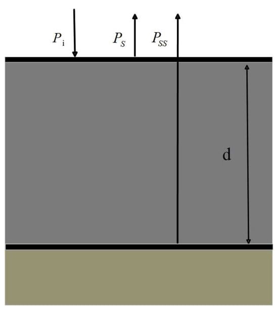
Figure 1.
Radar transmitting electromagnetic wave schematic diagram subscripts. is the incident power, and denote the surface and subsurface reflected power, respectively.
2.2. Current Status of Subsurface Information Extraction Technology
Current research on subsurface layer extraction mainly focuses on stratified regions of Earth and Mars, and can be categorized into two types. The first type involves statistical and machine learning methods. Ref. [10] used the Viterbi Algorithm (VA) for multi-layer boundary detection in Earth’s Ground-Penetrating Radar (GPR) data. However, the VA has its limitations because it assumes that layer boundaries always start from the leftmost side of the radargram. For Martian radargrams, layer boundaries might only span a small portion of the image. Additionally, the VA may struggle with local irregularities or nonlinear features in radargrams. In contrast, Ref. [11] employed the Markov-chain Monte Carlo method (MCMC) for inferring layer boundaries. The MCMC is an iteration-based algorithm that gradually approaches the target distribution through repeated sampling processes. For Mars’s complex subsurface stratification, the convergence speed is slow. Ref. [12] suggested using Hidden Markov Models (HMMs) to model the radar responses of layer boundaries, and used the VA for the automated detection of layer boundaries in radargrams. However, in HMMs, each state (such as the presence or absence of layer boundaries) is associated with the reflected signals. Weak reflective layers with a lower signal strength may have lower corresponding observational probabilities, resulting in lower transitional probabilities in these areas. Therefore, this algorithm might not accurately identify weak reflective layers.
The second type encompasses signal processing and image processing methods. Ref. [13] combined the Continuous Wavelet Transform (CWT) and the DBSCAN clustering algorithm for three-dimensional reconstruction of subsurface reflectors in the Promethei-Lingula region. This technique is primarily suited for areas where reflectors are more dispersed. The radargram images of Martian Polar Layered Deposits (PLDs) indicate frequent and closely packed reflectors, so this method is less appropriate. Martian subsurface detection based on the Steger algorithm [14] can detect layers with a small spacing. It essentially involves the detection of curves by extracting center lines based on pixel values. The signal strength of the weak reflection layer is usually very low, close to the level of background noise, making it difficult to distinguish from noise. The accuracy and connectivity of reflector detection still need to be improved. In the following section, a new algorithm will be proposed to accurately extract the stratification of Martian polar regions.
3. Automatic Detection Algorithm
Figure 2 shows a flowchart of the proposed automatic detection algorithm. It consists of two main parts: mapped enhancement denoising and subsurface reflector detection. Finally, the peak points of the detected underground layers are connected into continuous layers using proximity checks.
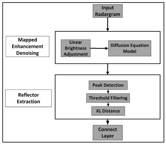
Figure 2.
Flowchart of the automatic method for Martian subsurface reflector detection.
3.1. Mapped Enhancement Denoising
This step aims to diminish the background noise in the radargrams and enhance the signature of linear features, preparing for subsequent subsurface reflector detection with the mapped enhancement denoising algorithm. It consists of two parts, the linear brightness adjustment based on image histogram peaks, and the image denoising and edge enhancement based on fourth-order partial differential equations using AOS operators [15].
3.1.1. Linear Brightness Adjustment
To enhance the contrast of radargrams, it is necessary to perform a brightness adjustment. The input radar backscatter power map is linearly normalized to the range of 01~255, which makes radargrams easier to observe and analyze. It is logarithmically processed according to (1) to expand the contrast between the light and dark areas in the radargram.
The following linear mapping effectively removes non-zero values by mapping them to the appropriate range.
where is the mapping slope, which defines the proportional relationship between the input and output values. It is computed as
The percentile in (3) is the peak value of the distribution histogram of the current image’s pixel values, that is, the most frequently occurring pixel value. In (2), is the mapping intercept, used to adjust the baseline in the mapping process, and is computed as
The radargrams of orbit 00505101 and orbit 00520501 were used to evaluate the effect of the linear brightness adjustment. The standard deviation is an important indicator for measuring the distribution range of image pixel values. A higher standard deviation usually means that the image has a higher contrast. Figure 3b,d show the processed images, while Figure 3a,c show them after a linear brightness adjustment, with a significant increase in the standard deviation and contrast compared to before processing.
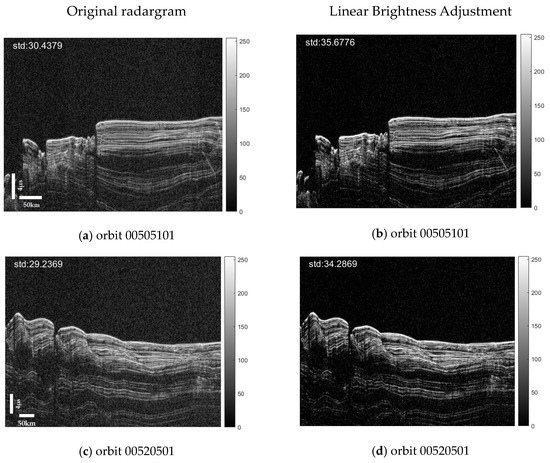
Figure 3.
Results of linear brightness adjustment.
3.1.2. Denoising of Radargrams
- (A)
- Denoising Algorithm based on Fourth-order diffusion equation
Before detecting the subsurface layers, a fourth-order partial differential equation (PDE) diffusion model was used for image denoising to eliminate the influence of random noise in radargrams on underground layered signals. If the radargram is treated as a two-dimensional function, , the noise is irregular fluctuations superimposed on the image function. By choosing an appropriate PDE model to describe this fluctuation, we can “diffuse” or “smooth” these irregularities while preserving the main features of the image, such as edges and textures. The diffusion equation is expressed as
where represents the image intensity, is the iteration time, and is a nonlinear diffusion function that depends on image gradients . is a Gaussian smoothing kernel and is the standard deviation that controls the degree of smoothness.
Equation (5) contains two independent partial differential operators in the x and y directions. Thus, a parallel splitting method [16] based on the additive operator splitting (AOS) [15] is used to divide the two-dimensional diffusion process into two independent processes: row diffusion and column diffusion [17]. The discrete iterative equations are as follows:
where and represent the results of row diffusion (horizontal direction) and column diffusion (vertical direction) in the n + 1 iteration, respectively, and represent the row and column indices, respectively, represents the time step, and are discrete second-order derivative operators, and and are diffusion coefficients related to the image gradient.
where represents the convolution of a Gaussian filter with image , and represents an infinitely small positive number, which is used to prevent the denominator from being 0. and are the local characteristic function of images in horizontal (X direction) and vertical (Y direction) directions, expressed as
Finally, the two diffusion results are averaged as to ensure that diffusion effects in each direction are appropriately considered. Since and are symmetric positive definite operators, the AOS operator is unconditionally stable. For each time step, (6) is performed iteratively until the image change between adjacent iterations is less than a certain threshold.
- (B) Denoising Results
This part will demonstrate the results with the above denoising algorithm based on the fourth-order diffusion equation, and quantitatively discuss the performance of the algorithm. The average variance was evaluated for images without layered information, while the average contrast was evaluated for images containing underground layers. The average contrast was measured using two statistical indicators: the grayscale co-occurrence matrix (GLCM) and contrast [18]. GLCM is a statistical method used to analyze texture features in images, which indicates the spatial relationship between grayscale values in the image. The contrast quantifies the local changes between grayscale levels, expressed as
where represents the frequency or probability of a pixel with grayscale value appearing next to the pixel with grayscale value at a specified distance and direction. N is the number of grayscale levels. This formula calculates the square of the difference in grayscale values between pixel pairs, weighted by their frequency of occurrence. is the square of the difference in pixel intensity values between and (the greater the difference, the higher the contrast). It examines the frequency at which a pair of pixels appears together in a specific direction and distance. A high contrast means significant grayscale changes, which are usually associated with clear textures or edges.
We performed the denoising process on the radargram of orbit 00505101 as shown in Figure 4a. The upper blue box outlines the non-layered region for the computation of average variance, which included random noise, as shown in Figure 4a. Figure 4b shows that the average variance rapidly decreased in the first eight iterations and then stabilized, indicating that the denoising level in this region was gradually converging [19]. Therefore, in terms of denoising, for the first eight iterations the noise continued to decrease, and the noise level tended to stabilize after eight iterations. Figure 4c shows that the average contrast value decreased by more than 50% after seven iterations. If the iterations continued, the layered information would be lost [18], which would further affect the accuracy of the subsurface reflector detection. Therefore, in this study, the number of iterations was set to seven.
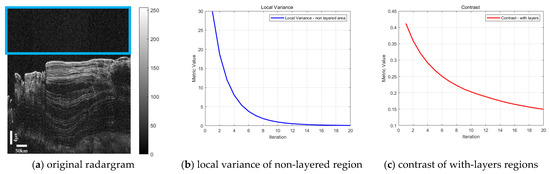
Figure 4.
The variation curve of variance and contrast with iteration (orbit 00505101). The metric values in (b,c) are the values of the local variance and the contrast. The upper blue box outlines the non-layered region for the computation of average variance.
Based on the runtime and image quality, it is necessary to choose an appropriate number of iterations. The unified selection of iteration times for this study was seven. The final preprocessed image is shown in Figure 5, taking orbit 00505101 and orbit 00221401 as examples, and they of the NPLDs and the SPLDs, respectively. Among them, (a) and (d) are the original graphs, (b) and (e) are the graphs after linear brightness adjustment, and (c) and (f) are the partial enlarged images after seven iterations of the fourth-order partial differential diffusion equation. It can be observed that the noise in (b) and (e) was significantly removed, while in (c) and (f) there was a further removal of the noise while image details were maintained.
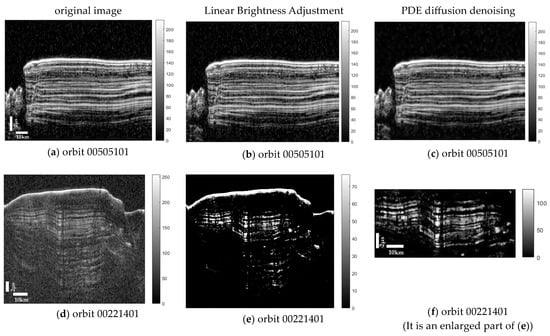
Figure 5.
The preprocessed results step by step for SHARAD radargrams of different orbits.
3.1.3. Performance Evaluation of Denoising Process
The SSIM (Structural Similarity Index Measure) is now used as one of the indicators to evaluate the denoising performance of fourth-order PDE diffusion, expressed as [20]
where , are the original image and the processed image, respectively. is the luminance matrix, is the contrast matrix, and is the structure matrix. These matrixes are expressed as follows:
where , are pixel mean values of each image; , are the pixel standard deviations; and is the covariance of the two images.
We used the clutter simulation images of orbit 00505101 and orbit 00520501 as original noise free images, and added random Gaussian noise to obtain noisy images (https://ode.rsl.wustl.edu/mars/datasets, accessed on 9 September 2023). Both BM3D filters and fourth-order PDE diffusion were used for image denoising. The evaluation indicators included the SSIM (Structural Similarity Index Measure), the PSNR (Peak Signal-to-Noise Ratio), and the time consumption. The results are shown in Table 1, which indicated that the fourth-order diffusion equation based on the AOS operator had a better denoising effect than BM3D filter. In addition, the time consumption of PDE diffusion denoising was also lower.

Table 1.
Comparison of SSIM, PSNR, and running time of orbit 00505101 and orbit 00520501.
3.2. Reflector Extration
- (a)
- Peak detection
In geological or geophysical data, the boundary of layers is usually manifested as a sudden change in signal intensity. Peak detection helps identify these mutation points and determine the position of layers. Therefore, peak detection can be used to extract peak points below the surface echo, and then locate the hierarchical positions.
The radar emits broadband electromagnetic wave signals along the orbit and receives the scattered echoes from the Martian surface and underground interface to form radargrams. The maximum power of each echo typically comes from the surface. Considering the continuity of the surface, determining the position of surface echoes in radargrams should consider the following two scenarios. (1) If the position of the maximum value in the current sequence differs by less than five pixels from the surface position detected in the previous sequence, the position of this maximum value is the right position of the surface echo. This situation may occur in areas with relatively flat terrain, with no significant terrain undulations or other surface features such as large rocks, ravines, or potholes. (2) If the position of the maximum value in the current sequence differs by more than five pixels from the surface position detected in the previous sequence, the first point with an intensity greater than five times the average value of the sequence is the position of the surface echo. This situation may occur in areas with complex terrain or significant topographic changes such as steep slopes, cliffs, large rocks, or other surface structures. These terrain features may cause significant changes in the position of the maximum value of radar echoes.
After finding the location indicating the echo based on the above method, the peak detection function was used to find some peaks of each echo sequence. Figure 6 is an example of peak detection below the surface echo, which represents frames 707, 768, 867, and 1048 of orbit 00505101.
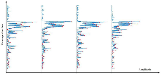
Figure 6.
Example of peak extraction. Red dots indicate detected peaks.
Since the subsurface radar antenna on the orbiter detects changes in dielectric properties, any change in ground composition will yield a strong return. As the peak points extracted in the above steps were all peak points below the surface, both layered and non-layered peak points were extracted. Therefore, further screening was needed to reduce the non-layered peak points. The next step involves threshold filtering of the detected peak points beneath the surface layer. For each radar echo sequence , (12) is used to compute the local coefficients, which is the relative intensity of a numerical change within a local window.
where the local window is set to 30 [21]. The peak detection function is used to detect the peak of the sequence C. For the detected peak values, the standard deviation is calculated as the threshold to remove false peaks. The filtered results of Figure 6 are shown in Figure 7, which indicates that the peak points extracted underground were screened.

Figure 7.
After threshold filtering. Red dots indicate detected peaks.
- (b) Feature extraction
In addition to the subsurface stratification, the peaks extracted from the above process include non-stratified points. In this session, the KL (Kullback–Leibler) divergence graph is used to further refine and filter out these non-stratified peak points. KL divergence is a method for measuring the difference between two probability distributions [22].
In this application, it is used to detect anomalies or features in images. The calculation of involves the KL distance between the actual distribution S of amplitude within an overlapping sliding window of size and the theoretical distribution of the fitted non-layered region within the window. A higher KL divergence value indicates a greater difference between the actual distribution S and the non-layered region distribution N. According to [23], the gamma distribution is most suitable for describing the characteristics of radar signals, so samples of different target categories (such as non-layered and layered areas) can be modeled using the gamma distribution. Therefore, the gamma distribution was used for fitting S and N.
The KL divergence value for each pixel in the image was calculated to assess its similarity to the surrounding pixels. In this paper, the KL divergence was computed as
where represents the pixel value of the row and column in the sliding window, and represents the probability of the gamma distribution followed by pixel values within a local window of centered on . represents the probability of the non-layered region distribution being in the same window. In this study, in the non-layered region and in the underground layers were both considered as gamma distributions, and the probability density function of the gamma distributions is expressed as
where is the random variable and is the gamma function. The parameters and are the shape and scale parameters, respectively. They were calculated based on the geometric and arithmetic mean of the pixel values within the window as
where is the di-gamma function and is the mean in the local window . The size of the window was determined based on the empirical spatial distribution of Martian subsurface features [23]. Generally, the subsurface features have a broader distribution or continuity in the azimuthal direction, i.e., the horizontal direction, where changes are gradual. To capture this horizontal continuity or change, a larger azimuthal window is needed. On the other hand, the subsurface features in the vertical or range direction may change abruptly, such as transitioning from one ice layer to another, or to bedrock. Hence, in the range direction, i.e., the vertical direction, changes are steep. These abrupt changes do not require a large window to capture them as they are spatially confined. In this paper, the window size was set to based on our experience.
In order to calculate the scale parameter α and shape parameter β of the non-layered region, which is always distributed at the top of the input radargram, the samples from 0 to the first echo of the surface reflection need to be extracted. Thus, the sample numbers of each A-scan channel were
where is the index of the surfaced echo, is the tolerance value for the first echo detection, and is the number of columns in the original radargram. In this study, was set to 15 based on our experience.
The KL divergence of S and N was then computed. The higher the KL divergence value, the greater the difference between the actual distribution S and the non-layered area distribution N, indicating a greater likelihood of being a layered area. Based on the final KL value, a threshold process generates a binary encoded map to determine the presence of subsurface reflectors, as per Equation (17). Through some experiments, we determined the threshold as 50, and Figure 8 shows the binary encoded map.
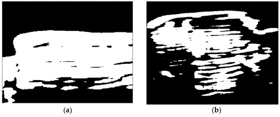
Figure 8.
KL map of orbit 00505101 (a) and orbit 00221401 (b).
Figure 8 shows the KL map of orbit 00505101 and orbit 00221401. Their original radargrams are shown in Figure 5. Thus, the KL map can particularly highlight the region with underground structures. Finally, the detected peak points were multiplied by the KL map, as shown in Figure 9.
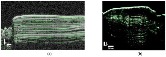
Figure 9.
Peak detection result of orbit 00505101 (a) and orbit 00221401 (b).
Figure 9 shows the results of peak detection in orbit 00505101 and orbit 00221401. The green color marks the location of the detected peak point. It can be seen from Figure 9 that the specific location of the peak point can be well detected for tight layers, and the location of layers can also be detected in some deeper areas.
- (c)
- Connecting peak points
The final step involves processing the coordinate set of the peak matrix into multiple layers, using proximity checks to determine if the points are in the same layer. We calculate the Euclidean distance of all detected peak points. If the distance is less than , they are in the same layer. is related to the frequency and bandwidth of SHARAD, expressed as Equation (18) [12,24].
where is the ceil operator. For SHARAD, the sampling frequency = 26.67 MHz, the bandwidth , and the SNR is approximately 17 dB [25]. Thus, the proximity . The final connected result of Figure 9 is shown in Figure 10.
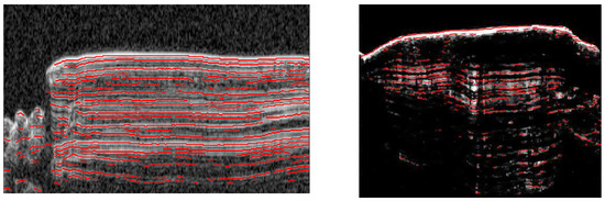
Figure 10.
Orbit 00505101 peak point connection.
4. Performance Analysis
4.1. Calculation of Missed Detection Rate and False Detection Rate
When evaluating the accuracy of subsurface reflector detection algorithms, it is common to use datasets with known labels for validation [26]. However, this method was not applicable due to the lack of standard labeled data for Martian polar subsurface layers. Another evaluation method involves assessing algorithm performance based on the number of extracted layers [12,27], but this approach is not suitable for algorithms based on peak detection. For peak detection algorithms, more appropriate evaluation criteria include detection accuracy, peak recognition ability, and false alarm rate. Therefore, using visual identification to evaluate the number of detected peak points offers a more precise way to differentiate between missed and falsely detected peaks, providing a more accurate method of assessment.
Therefore, to verify the accuracy in this study, visual identification results were used. For visual identification we used Adobe Illustrator 2021 software to meticulously annotate and evaluate inspection points to verify their accuracy. Here, the evaluation metric is not based on the number of detected layers, but on the count of peak points. The false detection rate and the missed detection rate were used for the evaluation [28].
where represents the number of false peak points, is the count of accurately detected peak points, and is the count of missed peak points.
Figure 11 shows the detection results of three SHARAD radargrams, where Figure 11a,b are NPLDs, and Figure 11c shows SPLDs. The basal unit structure of the Martian North Pole generally exhibits some ambiguous areas on the radargrams, such as the bottom region of Figure 11a,b. These basal structures are not the stratified structure, and this algorithm accurately neglected them. Some missed detections of deeper layers, marked in the red box, were mainly due to the lower SNR (signal-to-noise ratio), and some false detections of shallow layers, marked in the blue box, were mainly due to the smaller interval. The interlayer spacing in the image was minimized to an interval of approximately five pixels. Moreover, Figure 11c indicates that both the miss rate and false detection rate in the SPLDs region were higher than in the NPLDs region. The reason is that SHARAD images of the SPLDs often display near-surface scattering phenomena, creating a diffuse, fog-like appearance that obscures the underlying reflective stratified layers [29]. Additionally, the radar attenuation losses in the SPLDs were significantly greater than those in the NPLDs [29], resulting in large areas of white, blurred brightness in the images, as in Figure 12. In terms of peak detection, the lower signal-to-noise ratio (SNR) in the SPLDs was due to a problem with the orbital data [30], which in turn led to increased missed and false detection rates.
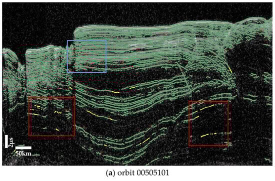
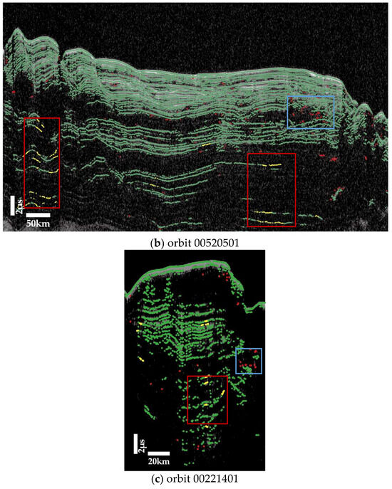
Figure 11.
Visual identification and verification using Adobe Illustrator. The yellow marks represents the peak point of missed detections, while the red marks represents the peak point of false detections.
Figure 12.
Orbit 00221401. The red box represents the detection area.
Table 2 shows the detection accuracy parameters of three SHARAD radargrams. The missed detection rate and false detection rate were both below 5%. For the NPLDs with a small interlayer spacing, the missed detection rate and false detection rate were very low, with a miss rate of less than 1%. Compared with the extraction results of the NPLDs, the missed detection rate and false detection rate of the extraction results of the SPLDs were increased, but both were below 5%. Therefore, the threshold processing showed excellent performance in terms of reflector detection. This method demonstrates significant adaptability, accurately identifying the position of strata in each column of the image, and maintaining a consistent detection capability even with increasing depth. In addition, its high sensitivity makes it particularly suitable for identifying complex underground formations. It effectively distinguishes and identifies subtle hierarchical differences, even in radargrams with a very small interlayer spacing.
Table 2.
Accuracy of the proposed technique for three regions.
4.2. Comparative Analysis of Reflection Detection Results with Other Literature
Figure 13 shows a comparison of the detection results of orbit 00520501 and orbit 00528401 with our algorithm and [12]. The extracted layers with our algorithm are clearer, and show a good improvement in the continuity between layers.
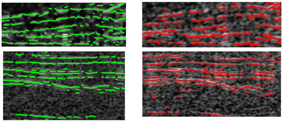
Figure 13.
Comparison of the subsurface layer with different algorithms. The left is the algorithm of this paper and the right is the algorithm of Ref. [12]. The above row is orbit 00520501, and the bottom row is orbit 00528401.
In addition, the algorithm described in this paper and the algorithm of [13] were applied to the NPLDs orbit 00520501 and the SPLDs orbit 00221401. The comparative results in Figure 14 indicate that the algorithm presented in this paper could detect more layers.
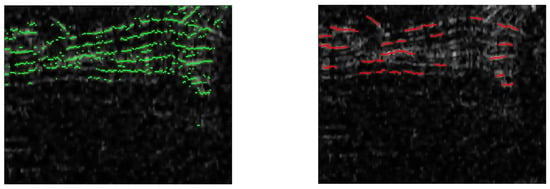
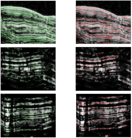
Figure 14.
Extract comparison with different algorithms. The left is the algorithm of this paper and the right is the algorithm of Ref. [13]. The rows from top to bottom are orbit 00520501, orbit 00520501, orbit 00221401, and orbit 00221401.
Moreover, since the wavelet transform algorithm in [13] is based on wavelet transform peak detection, Table 3 presents the comparison results, indicating that compared to [13], the algorithm in this paper performs better in terms of the missed detection rate, but is slightly inferior in terms of the false detection rate. Although a lower missed detection rate is often accompanied by a higher false detection rate, this phenomenon may be due to the preprocessing step not completely removing the noise without stratification.
Table 3.
Comparison of detection results with [13].
The above comparison of images and quantitative evaluation metrics demonstrates the effectiveness of our new algorithm. (1) Through threshold filtering, it retains valid peak points and discards most non-stratified peaks, thereby enhancing the accuracy. (2) Unlike traditional line detection methods, such as the Steger algorithm [27], this algorithm is based on peak detection, allowing it to identify weak reflective layers. (3) As shown in Figure 13, there is an improvement in continuity compared to [12]. (4) Compared with [13], the missed detection rate decreased significantly.
To test the applicability of this algorithm in other regions of Mars, two orbiter’s radargram images in mid-latitude areas were tested. Figure 15a shows the detection result of orbit 00320802 in Mars’s Zephyria Planum [17], and Figure 15b shows the detection result of orbit 00320802 in the Elysium–Utopia Region [31,32]. The assessment explicitly excluded areas with more ambiguous subsurface structures. Although there were some false detections at the locations indicated by the arrows, the subsurface layers were still accurately detected, as shown in the Figure 15. This demonstrates the algorithm’s applicability and value in non-polar regions of Mars.
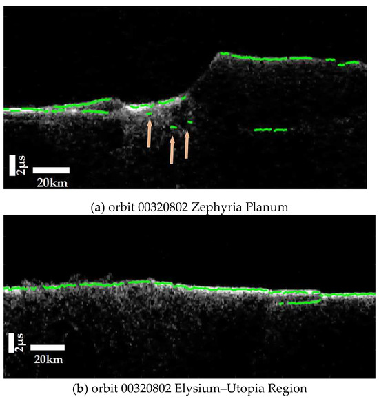
Figure 15.
The extractions from Zephyria Planum and Elysium–Utopia Region. The arrows mark the false detections.
5. Conclusions
This paper developed an automatic algorithm for detecting subsurface layers using SHARAD images, especially for the detection of dense stratification at different depths in Martian polar regions. The main contribution of this article is the development of a peak extraction method based on threshold processing, which is used to effectively detect underground reflectors in radar echo signals. Firstly, this method is particularly suitable for identifying complex underground structures. By combining the threshold processed peak with the extracted features, it not only exhibits high adaptability to different geological structures, but also has extremely high sensitivity to weak signals. Secondly, combining the steps of mapped enhancement denoising and peak detection in this algorithm, it can accurately identify the positions of underground layers, and can even detect weak reflectors in deep areas or dense layers with small interlayer spacing. In addition, the strata detected using this method exhibit better continuity horizontally. Overall, the use of this algorithm has improved the overall performance and accuracy of radargrams in revealing underground structures.
Author Contributions
Conceptualization and methodology, H.Y.; validation and writing, X.S.; supervision, H.Y. All authors have read and agreed to the published version of the manuscript.
Funding
This work was funded by the National Natural Science Foundation of China No. 62271152.
Data Availability Statement
The original data presented in the study are openly available in SHARAD data at https://ode.rsl.wustl.edu/mars/datasets, accessed on 9 September 2023.
Conflicts of Interest
The authors declare no conflicts of interest.
References
- Cutts, J.A. Nature and origin of layered deposits of the Martian polar regions. J. Geophys. Res. 1973, 78, 4231–4249. [Google Scholar] [CrossRef]
- Picardi, G.; Biccari, D.; Cicchetti, A.; Seu, R.; Plaut, J.J.; Johnson, W.T.K.; Jordan, R.L.; Gurnett, D.A.; Orosei, R.; Zampolini, E.M. Mars Advanced Radar For Subsurface And Ionosphere Sounding (MARSIS). Planet. Space Sci. 2003, 52, 149–156. [Google Scholar] [CrossRef]
- Seu, R.; Phillips, R.J.; Biccari, D.; Orosei, R.; Masdea, A.; Picardi, G.; Safaeinili, A.; Campbell, B.A.; Plaut, J.J.; Marinangeli, L.; et al. SHARAD sounding radar on the Mars Reconnaissance Orbiter. J. Geophys. Res. 2007, 112. [Google Scholar] [CrossRef]
- Fan, M.; Lyu, P.; Su, Y.; Du, K.; Zhang, Q.; Zhang, Z.; Dai, S.; Hong, T. The Mars Orbiter Subsurface Investigation Radar (MOSIR) on China’s Tianwen-1 Mission. Space Sci. Rev. 2021, 217, 8. [Google Scholar] [CrossRef]
- Wen, Y.; Sun, J.; Guo, Z. A new anisotropic fourth-order diffusion equation model based on image features for image denoising. Inverse Probl. Imaging 2022, 16, 895–924. [Google Scholar] [CrossRef]
- Dabov, K.; Foi, A.; Katkovnik, V.; Egiazarian, K.O. Image Denoising by Sparse 3-D Transform-Domain Collaborative Filtering. IEEE Trans. Image Process. 2007, 16, 2080–2095. [Google Scholar] [CrossRef]
- Smith, D.E.; Zuber, M.T.; Frey, H.V.; Garvin, J.B.; Head, J.W.; Muhleman, D.O.; Pettengill, G.H.; Phillips, R.J.; Solomon, S.C.; Zwally, H.J.; et al. Mars Orbiter Laser Altimeter: Experiment summary after the first year of global mapping of Mars. J. Geophys. Res. 2001, 106, 23689–23722. [Google Scholar] [CrossRef]
- Byrne, S. The Polar Deposits of Mars. Annu. Rev. Earth Planet. Sci. 2009, 37, 535–560. [Google Scholar] [CrossRef]
- Smith, I.B.; Putzig, N.E.; Holt, J.W.; Phillips, R.J. An ice age recorded in the polar deposits of Mars. Science 2016, 352, 1075–1078. [Google Scholar] [CrossRef]
- Smock, B.; Wilson, J.N. Efficient multiple layer boundary detection in ground-penetrating radar data using an extended Viterbi algorithm. In Proceedings of the Detection and Sensing of Mines, Explosive Objects, and Obscured Targets XVII, Maryland, MD, USA, 10 May 2012. [Google Scholar]
- Lee, S.; Mitchell, J.E.; Crandall, D.J.; Fox, G.C. Estimating bedrock and surface layer boundaries and confidence intervals in ice sheet radar imagery using MCMC. In Proceedings of the 2014 IEEE International Conference on Image Processing (ICIP), Paris, France, 27–30 October 2014; pp. 111–115. [Google Scholar]
- Carrer, L.; Bruzzone, L. Automatic Enhancement and Detection of Layering in Radar Sounder Data Based on a Local Scale Hidden Markov Model and the Viterbi Algorithm. IEEE Trans. Geosci. Remote Sens. 2017, 55, 962–977. [Google Scholar] [CrossRef]
- Xiong, S.; Muller, J.-P. Automated reconstruction of subsurface interfaces in Promethei Lingula near the Martian south pole by using SHARAD data. Planet. Space Sci. 2019, 166, 59–69. [Google Scholar] [CrossRef]
- Steger, C. An Unbiased Detector of Curvilinear Structures. IEEE Trans. Pattern Anal. Mach. Intell. 1998, 20, 113–125. [Google Scholar] [CrossRef]
- Weickert, J. Applications of nonlinear diffusion in image processing and computer vision. Acta Math. Univ. Comenianae. New Ser. 2000, 70, 33–50. [Google Scholar]
- A parallel splitting-up method for partial differential equations and its applications to Navier-Stokes equations. Math. Model. Numer. Anal. 1992, 26, 673–708. [CrossRef]
- Weickert, J.; Romeny, B.M.t.H.; Viergever, M.A. Efficient and reliable schemes for nonlinear diffusion filtering. IEEE Trans. Image Process. A Publ. IEEE Signal Process. Soc. 1998, 7, 398–410. [Google Scholar] [CrossRef] [PubMed]
- Beura, S.; Majhi, B.; Dash, R. Mammogram classification using two dimensional discrete wavelet transform and gray-level co-occurrence matrix for detection of breast cancer. Neurocomputing 2015, 154, 1–14. [Google Scholar] [CrossRef]
- Lee, J.-S. Digital Image Enhancement and Noise Filtering by Use of Local Statistics. IEEE Trans. Pattern Anal. Mach. Intell. 1980, PAMI-2, 165–168. [Google Scholar] [CrossRef] [PubMed]
- Wang, Z.; Bovik, A.C.; Sheikh, H.R.; Simoncelli, E.P. Image quality assessment: From error visibility to structural similarity. IEEE Trans. Image Process. 2004, 13, 600–612. [Google Scholar] [CrossRef]
- Mouginot, J.; Pommerol, A.; Kofman, W.; Beck, P.; Schmitt, B.; Hérique, A.; Grima, C.; Safaeinili, A.; Plaut, J.J. The 3–5 MHz global reflectivity map of Mars by MARSIS/Mars Express: Implications for the current inventory of subsurface H2O. Icarus 2010, 210, 612–625. [Google Scholar] [CrossRef]
- Lin, J. Divergence measures based on the Shannon entropy. IEEE Trans. Inf. Theory 1991, 37, 145–151. [Google Scholar] [CrossRef]
- Ilisei, A.-M.; Bruzzone, L. Automatic classification of subsurface features in radar sounder data acquired in icy areas. In Proceedings of the 2013 IEEE International Geoscience and Remote Sensing Symposium—IGARSS, Melbourne, VIC, Australia, 21–26 July 2013; pp. 3530–3533. [Google Scholar]
- Barton, D.K.; Ward, H.R. Handbook of Radar Measurement; Artech House: Norwood, MA, USA, 1969; pp. 199–240. [Google Scholar]
- Campbell, B.A.; Putzig, N.E.; Carter, L.M.; Morgan, G.A.; Phillips, R.J.; Plaut, J.J. Roughness and near-surface density of Mars from SHARAD radar echoes. J. Geophys. Res. Planets 2013, 118, 436–450. [Google Scholar] [CrossRef]
- Varshney, D.; Rahnemoonfar, M.; Yari, M.; Paden, J.D.; Ibikunle, O.; Li, J. Deep Learning on Airborne Radar Echograms for Tracing Snow Accumulation Layers of the Greenland Ice Sheet. Remote. Sens. 2021, 13, 2707. [Google Scholar] [CrossRef]
- Ferro, A.; Bruzzone, L. Automatic Extraction and Analysis of Ice Layering in Radar Sounder Data. IEEE Trans. Geosci. Remote Sens. 2013, 51, 1622–1634. [Google Scholar] [CrossRef]
- Liu, X.; Fa, W. A Fully Automatic Algorithm for Reflector Detection in Radargrams Based on Continuous Wavelet Transform and Minimum Spanning Tree. IEEE Trans. Geosci. Remote Sens. 2022, 60, 4601620. [Google Scholar] [CrossRef]
- Hashmeh, N.A.; Whitten, J.L.; Russell, A.T.; Putzig, N.E.; Campbell, B.A. Comparable Bulk Radar Attenuation Characteristics Across Both Martian Polar Layered Deposits. J. Geophys. Res. Planets 2022, 127, e2022JE007566. [Google Scholar] [CrossRef]
- Whitten, J.L.; Campbell, B.A. Lateral Continuity of Layering in the Mars South Polar Layered Deposits From SHARAD Sounding Data. J. Geophys. Res. Planets 2018, 123, 1541–1554. [Google Scholar] [CrossRef]
- Nunes, D.; Smrekar, S.E.; Safaeinili, A.; Holt, J.W.; Phillips, R.J.; Seu, R.; Campbell, B.A. Examination of gully sites on Mars with the shallow radar. J. Geophys. Res. 2010, 115. [Google Scholar] [CrossRef]
- Alberti, G.; Castaldo, L.; Orosei, R.; Frigeri, A.; Cirillo, G. Permittivity estimation over Mars by using SHARAD data: The Cerberus Palus area. J. Geophys. Res. 2012, 117. [Google Scholar] [CrossRef]
Disclaimer/Publisher’s Note: The statements, opinions and data contained in all publications are solely those of the individual author(s) and contributor(s) and not of MDPI and/or the editor(s). MDPI and/or the editor(s) disclaim responsibility for any injury to people or property resulting from any ideas, methods, instructions or products referred to in the content. |
© 2024 by the authors. Licensee MDPI, Basel, Switzerland. This article is an open access article distributed under the terms and conditions of the Creative Commons Attribution (CC BY) license (https://creativecommons.org/licenses/by/4.0/).