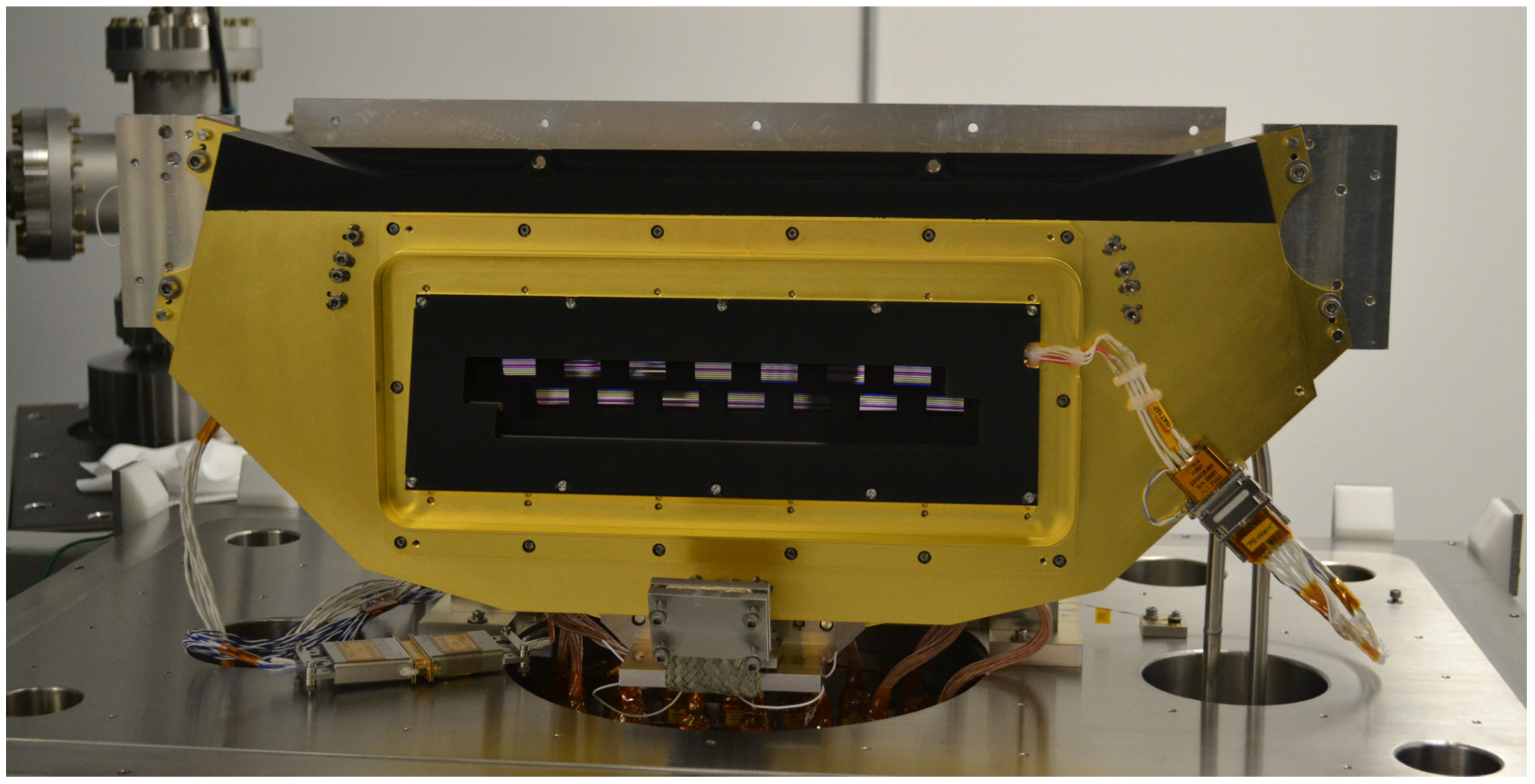
Article

Prelaunch Spectral Characterization of the Operational Land Imager-2

1
NASA/GSFC Biospheric Sciences Laboratory, Greenbelt, MD 20771, USA
2
Ball Aerospace and Technologies, Boulder, CO 80301, USA
3
Bay Engineering Innovations, Inc., Boulder, CO 80301, USA
4
Northrup Grumman, Sterling, VA 20166, USA
5
Hexagon US Federal, Chantilly, VA 20151, USA
6
Fibertek, Inc., Herndon, VA 20171, USA
7
Genesis Engineering Solutions, Inc., Lanham, MD 20706, USA
*
Author to whom correspondence should be addressed.
Work was performed while at a.i. solutions, Inc., Lanham, MD 20706, USA.
Remote Sens. 2024, 16(6), 981; https://doi.org/10.3390/rs16060981
Submission received: 5 January 2024 / Revised: 20 February 2024 / Accepted: 25 February 2024 / Published: 11 March 2024

Abstract

:
The Landsat-9 satellite, launched in September 2021, carries the Operational Land Imager-2 (OLI-2) as one of its payloads. This instrument is a clone of the Landsat-8 OLI and its mission is to continue the operational land imaging of the Landsat program. The OLI-2 instrument is not significantly different from OLI though the instrument-level pre-launch spectral characterization process was much improved. The focal plane modules used on OLI-2 were manufactured as spares for OLI and much of the spectral characterization of the components was performed for OLI. However, while the spectral response of the fully assembled OLI was characterized by a double monochromator system, the OLI-2 spectral characterization made use of the Goddard Laser for Absolute Measurement of Radiance (GLAMR). GLAMR is a system of tunable lasers that cover 350–2500 nm which are fiber-coupled to a 30 in integrating sphere permanently monitored by NIST-traceable radiometers. GLAMR allowed the spectral characterization of every detector of the OLI-2 focal plane in nominal imaging conditions. The spectral performance of the OLI-2 was, in general, much better than requirements. The final relative spectral responses (RSRs) represent the best characterization any Landsat instrument spectral response. This paper will cover the results of the spectral characterization from the component-level to the instrument-level of the Landsat-9 OLI-2.

1. Introduction

The Operational Land Imager-2 (OLI-2) is the latest reflective band instrument in the Landsat series of imagers, launched aboard the Landsat-9 spacecraft in September 2021. Landsat-9 also carries a thermal band instrument, the Thermal Infrared Sensor-2 (TIRS-2), but TIRS-2 will not be covered in this paper. Both instruments are effectively clones of the OLI and TIRS carried on Landsat-8 and continue the Earth-imaging legacy of the Landsat program, now over 50 years long.
Knowledge of the spectral response of any remote sensing instrument is key to understanding and utilizing the data. This paper describes how the spectral characterization of OLI-2 was performed prior to launch. Traditionally the spectral characterization is performed with a monochromator system as was the case for Landsat-8 OLI [1] and Sentinel-2C/D Multi Spectral Instrument [2]. However, the OLI-2 instrument-level test was performed with the Goddard Laser for Absolute Measurement of Radiance (GLAMR). This paper describes the instrument test in detail and the validation performed to ensure GLAMR would meet the test requirements. It presents a summary of the spectral response data and provides links to the complete data sets. It shows some implications of the variation in spectral response across the instrument field of view and compares the absolute spectral response derived from GLAMR to the responsivity derived from the white-light calibration. Portions of the content of this paper have previously been presented at conferences and published in their proceedings [3].

1.1. Landsat OLI-2 Design

The Landsat-9 OLI-2 is a multispectral earth observing instrument with nine spectral bands; it has eight 30-m bands, and one 15-m panchromatic band (Table 1). The four-mirror nearly telecentric telescope has a 15° field of view. The pushbroom focal plane consists of 14 focal plane modules (FPMs) (Figure 1). Each module has 494 active imaging detectors (988 for the Pan band), so each of the multi-spectral bands consists of 6916 distinct imaging detectors. The visible and near-infrared (VNIR) spectral bands use Silicon (Si) PIN photodiodes and the shortwave infrared (SWIR) bands use Mercury-Cadmium-Telluride (HgCdTe) photodiodes.
Each detector array on each FPM is covered by a “butcher block” assembly of spectral filters to differentiate the spectral bands. The filter wafers were manufactured using a hardening process that minimized the absorption of water between layers [4]. These hardening processes reduce the possibility of a spectral shift in the filters on orbit. The filter sticks in each butcher block were each cut from a larger filter wafer. The filter wafers were all originally manufactured for OLI, and as a result, some of the OLI-2 modules share a source filter wafer with the OLI band. Similarly for the detector arrays, some OLI and OLI-2 modules share detectors manufactured in the same production lots. These manufacturing similarities increase the possibility that the spectral differences between the instruments will be small. Table 2 lists the wafer source of each module’s filter.
The focal plane assembly (FPA) window was a fully finished spare for OLI. The four telescope mirrors were manufactured as spares for OLI, though they did not have their final polishing or silver coating until being prepared for use in OLI-2.

1.2. Spectral Test Sets

The OLI-2 spectral response was characterized at several points along the instrument build: at the individual detector and filter wafer level, at the module level and at the instrument level. Because the OLI-2 was built with components originally built for the OLI, the earliest-in-development characterizations could not be repeated because the filters and wafers had already been cut and assembled into modules. In order to ensure the filter performance had not changed in the time since they were manufactured, the spectral transmission of filter witness samples was remeasured in 2016 and compared to the original measurements from 2008. The comparison showed that the center wavelength, as calculated from the midpoint between the 50% response points, shifted by less than 1.0 nm across all but one spectral band. The uncertainty in the comparison is on the order of +/−1.0 nm. The measured difference for Band 5 was 1.4 nm; since this band covers a transition region between spectrometers, gratings, detectors, and lamp sources, the large difference is attributed to measurement challenges rather than spectral change. With these data, there was high confidence that the spectral transmission of the flight filters did not change while in storage.
The reflectances of witness samples of the four mirrors were measured by the coating vendor, Quantum Coating, Inc, from 400 to 2500 nm and by Ball Aerospace from 300 to 400 nm and 2500 to 2700 nm. The spectral transmission of a witness sample of the focal plane assembly window was measured at five positions by Sonoma Photonics in 2010 and at three positions by Ball Aerospace in 2017 using a Cary 500 spectrometer. No significant aging of the window witness samples was observed.
At the module level, the intent of the characterization was to measure the out-of-band spectral response. Measurements were made of 12 of the 14 of the modules used on OLI-2 in 2010. See [1] for a description of the test. The out-of-band response for the two unmeasured modules were approximated based on their component-level measurements.
The final instrument-level spectral characterization took place in 2018 using the Goddard Laser for the Absolute Measurement of Radiance (GLAMR) as the source, rather than the double monochromator used for OLI characterization. GLAMR is a mobile NASA/Goddard-based spectral test facility, developed to facilitate the characterization and calibration of Earth remote sensing instruments. The tunable laser-based system provides a large, uniform source of monochromatic radiance between 380 and 2500 nm. The system will be described more fully in Section 2.
There are several advantages to using a GLAMR-like system over a traditional lamp-based monochromator system for spectral characterization. It provides a flood illumination of the focal plane, the illumination is unpolarized, the beam is spatially and spectrally uniform, the near delta-function wavelength can nominally be sampled at 0.1–1 nm intervals, and the source is monitored in real time. Since the GLAMR radiance is monitored with a calibrated radiometer, GLAMR can also provide absolute calibration. However, the absolute calibration capability was not a requirement for the characterization of OLI-2.

1.3. GLAMR

GLAMR is based on the NIST Spectral Irradiance and Radiance Calibrations using Uniform Sources (SIRCUS) facility [5]. The traveling version of SIRCUS (T-SIRCUS) was first used to characterize the spectral response of the solar reflective bands of Suomi National Preparatory Project (SNPP) Visible Infrared Imaging Radiometer Suite (VIIRS) [6]. T-SIRCUS went on to characterize the first Joint Polar Satellite System (JPSS-1) VIIRS in 2014 [7]. In 2016, the first GLAMR system was used to characterize the spectral response of JPSS-2 VIIRS [8] and Goddard’s Lidar, Hyperspectral and Thermal Imager (G-LiHT) [9]. Since the OLI-2 characterization in 2018, GLAMR has been used for the characterization of JPSS-3 VIIRS [10], JPSS-4 VIIRS, the Plankton, Aerosol, Cloud, ocean Ecosystem (PACE) Ocean Color Instrument (OCI) [11] and the L’Ralph visible imager on Lucy, a mission to the Trojan asteroids [12].
The GLAMR spectral range is covered by several configurations of custom-built Optical Parametric Oscillators (OPOs) and two commercial lasers. There are two OPO cavities on each OPO system, which can be configured for different wavelength ranges: the fundamental signal, the Idler and the Second Harmonic Generation (SHG) [13]. The OPOs are mode-locked pulsed pump sources while the two commercial systems are continuous wave sources. There are three optical benches, referred to as OPO Laser Alignment Facilities (OLAFs). OLAF1 and OLAF2 OPOs are pumped by a 532 nm 20 W Coherent Paladin neodymium vanadate laser mode-locked at 80 MHz and the OLAF3 OPOs are pumped by a 532 nm 35 W Coherent Paladin pump laser mode-locked at 76 MHz. The spectral ranges each of the OPO covers is provided in Table 3. Two commercial systems, the ARGOS by Aculight Corporation and the CLT by IPG Photonics Corporation, each sit on their own bench, and provide complete redundancy for wavelengths above 2185 nm.
The light from the laser systems is fiber-fed into the 30 in PFTE integrating sphere with a 12 in port. There are three fibers for different spectral ranges, all mounted in the sphere such that the first bounce will not exit the sphere port. The signal in the sphere is continuously monitored by a set of three radiometers to cover the full spectral range. The output of these radiometers, called sphere monitors, is fed back to the power stabilizer on the laser table to provide radiance-stabilized energy in the sphere. A second set of three radiometers is used to transfer the NIST radiance scale to the sphere monitors; these are referred to as the transfer radiometers. For both the sphere monitors and transfer radiometers, a Silicon (Si) detector radiometer is used to cover 300–1100 nm, an Indium-Gallium-Arsenide (IGA) detector radiometer covers 850–1600 nm, and an extended IGA (XIGA) is used for 1600–2500 nm.
Most control of the laser systems and shutters is performed via a custom-built Labview software interface. Displays provide real-time monitoring of radiometer signal and wavemeter wavelength as well as other key telemetry points. Wavelength steps are made by the software controlling temperatures of the nonlinear crystal ovens and positions of stages to adjust beam path through dispersion prisms and OPO cavity length, based on previously generated tuning parameter look-up tables. The telemetry from GLAMR, the data reported from the radiometers and wavemeters as well as shutter and laser statuses, are recorded at rates between 1 and 20 Hz. Time stamps are included with all the asynchronous telemetry streams. The data are recorded to text files, but also can be streamed directly to the telemetry system of instrument under test.
For an instrument test using GLAMR, the GLAMR integrating sphere is placed directly in front of the imaging instrument under test (Figure 2). The radiance from the sphere illuminates the imager. Each illuminated interval is bracketed by a dark interval, with the GLAMR shutter closed. Because the output of the radiometer is calibrated radiance, the images acquired can be used to determine the absolute responsivity of the imager as well as the relative spectral response.
The absolute radiometric scale for GLAMR is established and maintained using calibrated transfer radiometers, traceable to primary national radiometric standards at NIST [14]. Before and after an instrument measurement campaign, the GLAMR transfer radiometer calibration is tied to the Primary Optical Watt Radiometer (POWR). At NIST, a stabilized laser source is used to transfer the radiometric scale from POWR to the GLAMR transfer radiometers via another set of standard radiometers. This radiometric scale is transferred to the sphere monitors, a process called sphere calibration. A sphere calibration determines the ratio between the energy seen inside sphere by the sphere monitors and the energy seen outside the sphere by the transfer radiometers. Sphere calibrations are repeated before and after a measurement campaign to verify stability of the GLAMR system over the duration of the test.
The total uncertainty of the GLAMR system in 2018 includes the uncertainty of the NIST calibration from the summer of 2017, along with terms for sphere calibration repeatability, measurement noise and uniformity of the integrating sphere (Figure 3). The largest contributor to the uncertainty is the NIST calibration of the transfer radiometers, but the uncertainty in the repeatability of the sphere calibration was also significant.
The uncertainties provided by NIST are roughly 0.3% for Si radiometer calibration, 0.7% for the IGA radiometer calibration, and 4–6% for the XIGA radiometer calibration (k = 2) [15,16,17]. The sphere calibration repeatability was based on multiple sphere calibrations performed in the GLAMR lab. Over multiple days and with different laser sources, the sphere calibration was repeatable to 0.45% in the Si radiometer range, and 0.95% in the IGA radiometer range (2-sigma). The exercise was not performed for the XIGA range at the time, but it was assumed that the repeatability above 1600 nm would be similar to the IGA, so a placeholder value of 1% was used. Since 2018, it has been demonstrated that the repeatability for the entire GLAMR system is better than 0.1% outside of water vapor bands [18], so the 1% estimate was conservative. The measurement noise was estimated based on the stability required for the OLI-2 imaging time, 2 s. Based on the test data, the measurement noise across all wavelengths was 0.02% (2-sigma).
The uniformity of the sphere was based on a measurement from the NIST T-SIRCUS sphere in 2014. The GLAMR sphere and the NIST sphere are of similar design and manufacture, so it was believed this measurement was a sufficient proxy for the uniformity of the GLAMR sphere. The sphere was uniform to within 0.14% (2-sigma) as measured at 488 nm with a 1° field-of-view radiometer (Figure 4). Subsequent measurements have confirmed that the GLAMR sphere is uniform to better than 0.14% across all wavelengths.
The total GLAMR uncertainties for individual OLI-2 spectral bands are provided in Table 4. Since this test, significant effort has been made to reduce the total uncertainties across the whole spectral range [18], but the estimates here represent the state of the system in 2018.
The CLT performance is negatively affected by speckle, a result of the laser linewidth being too narrow to spectrally average the interference between the ensemble of optical paths reaching each point on the integrating sphere. The pattern is also time varying due to phase noise of the laser and mechanical vibration. This interference pattern results in non-uniform and time varying spatial patterns in the sphere, which increases the variance of the measurement. The effect of speckle on the measurement can be reduced by vibrating the input fiber spatially average the non-uniformity within the integration time of the detector [19]. GLAMR makes use of several electric toothbrushes, placed in contact with the metal-clad fiber coupled between the CLT and the sphere, to reduce the effect of speckle.

2. Spectral Measurements

2.1. Component-Level Characterization

For each component, the spectral response was measured individually before any parts were assembled. The spectral transmission of each filter wafer was measured at nine positions by filter provider, Barr Associates (now part of Materion). Relative spectral responses of witness detectors were measured in vacuum at 210 K by the detector provider, Raytheon Vision Systems (RVS). The spectral transmission of a witness sample of the focal plane assembly window was measured by Sonoma Photonics and was repeated by Ball Aerospace. The reflectance of witness samples of the four telescope mirrors was measured by Quantum Coatings and Ball Aerospace. The collection of optics response curves is shown in Figure 5. A system-level RSR was calculated based on analytically combining the transmission of the filter wafer and the response of the detectors that were used in the flight instrument. These were convolved with the reflectance of the four mirrors and the transmission of the focal plane assembly window. Figure 6 shows the predicted system level response for several bands. These results provided a baseline for the out-of-band response and uniformity of the spectral response.

2.2. Module-Level out-of-Band Characterization

The module-level spectral response was determined from the OLI-era measurements of each flight-qualified module. The telescope mirror reflectances and focal plane array window transmission (Figure 5) were convolved with the module-level responses to estimate a system-level response. The responses were averaged across the full module and then across all 14 flight modules to estimate a band-average response.
The band average out-of-band responses based on FPM-level measurements are shown in Figure 7. There are features in the data (Figure 7) that result from the test conditions as opposed to the instrument spectral response. The features are a result of order-sorting filter effects and in-band to out-of-band measurement effects. These are the same order-sorting and measurement effects seen in the OLI data since the same test set was used. See [1] for more details.
All three SWIR bands in Figure 6 exhibit higher out-of-band response in the spectral ranges corresponding to the other two SWIR band region than in the surrounding spectral regions. For example, the SWIR1 band response approaches 0.001 in the range corresponding to SWIR2, compared to about 0.0001 in the surrounding spectral regions. Additional pre-launch testing, experiments, and analysis for OLI indicated that this was crosstalk between the bands within the detector material. This crosstalk was expected for OLI-2 and has the same impact on the imagery. See [1] for the details.

2.3. Instrument-Level Characterization

The spectral response of the fully built OLI-2 was characterized in a thermal vacuum chamber under conditions that emulate the space-flight environment, by running the instrument at operational temperatures and in a vacuum environment. By measuring the spectral response in flight-like conditions, the reported results should capture any spectral changes due to temperature or environment. While comparisons were made to check the change in the spectral response between ambient and flight-light conditions and were found to negligible [4], the spectral response of record is the one determined under flight-light conditions. The GLAMR facility was the energy source for the instrument-level characterization.

2.3.1. Test Requirements on GLAMR

The GLAMR test replaced the use of a Ball double monochromator, and thus, test requirements were placed on the Goddard system to ensure OLI-2 could be characterized adequately for Ball to meet instrument test requirements. To meet most of the performance requirements (Table 5), GLAMR performed test scans in advance of deploying to Ball Aerospace to demonstrate compliance. This test served to verify that the GLAMR wavelength range and sampling was adequate, that the radiometric signal was stable over the required dwell time and GLAMR would provide sufficient signal to meet the SNR requirements. Figure 8 demonstrates compliance for several of the requirements by displaying the wavelength sampling, the GLAMR absolute radiance levels and the requirement radiance levels. The minimum radiance requirement was generally not satisfied below 700 nm due to the lower power available in the Second Harmonic Generation (SHG) OPO configuration used for those wavelengths. The spectral sampling and linewidth of the GLAMR system for specific ranges are provided in Table 6.

2.3.2. Consideration of Risk to Focal Plane

There was some concern that the energy originating from the pulsed laser source and viewed through the integrating sphere port could saturate or even damage the OLI-2 detectors. Two specific risks were considered, namely (1) that a “first-bounce”, high peak intensity laser pulse could escape the sphere and damage the OLI-2 detectors and (2) that the readout integrated circuit (ROIC) could saturate with the pulse peak intensity resulting in non-linear signal loss. The input to the GLAMR integrating sphere is designed such that a first-bounce should not be able to escape the sphere, and the theory says that the integrating sphere will serve to average and stretch the laser pulses such that the peak intensity leaving the sphere is a fraction of the laser pulse peak intensity. Two studies were developed to test the hypothesis.

2.3.3. Integrating Sphere Validation

The pulsed light illuminating an integrating sphere should be temporally averaged within the high-reflectance, uniformly scattering sphere coating. The time constant of the integrating sphere can be modeled by
τ = 2 D s π c ln ρ ¯
where Ds is the inner diameter of the sphere (0.762 m), c is the speed of light [3.0 × 10⁸ m/s2], and ρ ¯ is the effective reflectivity of the sphere (0.953) [20]. This produces a time constant of 33 ns, approximately three times the pulse repetition period of the source. As pulses of light are introduced into the sphere, the radiance at the output port reaches a limit cycle after a few time constants and the radiance varies by only ±20% from the average (Figure 9a); the high peak power 76 MHz pulses are contained in the sphere and never escape the sphere, as predicted by the model data.
An experiment was developed to test the integrating sphere model [21]. Two high-speed detectors and an oscilloscope were used to test the model. One 10 GHz detector measured the radiance exiting the sphere, the other detector measured the signal inside of the sphere on the wall near the first bounce. The normalized signal exiting the sphere is shown in Figure 9a, with the model results. The radiance exiting the sphere matches the model in both period and magnitude. Inside the sphere, the laser pulse is very apparent (Figure 9b) with an order of magnitude more power than outside the sphere.
Further test and modeling details are provided in [21]. The study confirmed that the energy exiting the sphere would not damage the OLI-2 focal plane. Further investigation of the other OLI-2 pre-launch calibration sources revealed that the peak radiance that OLI-2 would be exposed to by GLAMR would not exceed the radiance level of the brightest lamp being used in the standard lamp-illuminated integrating sphere calibration tests (referred to as the DSS) (Figure 10).

2.3.4. Damage Special Study

Additional verification was performed with a spare focal plane module. Ball Aerospace brought a flight-qualified module not slated for use in the OLI-2 instrument to Goddard in February 2017, along with the hardware needed to operate and characterize the module at standard operating conditions. A GLAMR test was designed to illuminate the module with the maximum power available at five different wavelengths for worst-case exposure scenarios (>30 min) and illuminate the NIR channel with energy at 868 nm with both the nominal GLAMR pulsed laser and an available Ti:Sapphire continuous wave laser. Before and after the module was exposed to the GLAMR system, standard calibrations were made using a lamp and integrating sphere system, the same system as was used to verify performance characteristics of the module in 2016.
The analysis of the module operability before and after the GLAMR exposure revealed no signs of damage and no changes in responsivity, dark noise or dark offset. The median signal-to-noise ratio (SNR) of the 494 detectors for each band was within 2.5% before and after exposure. The median responsivity for the NIR band illuminated separately with the pulse laser and with the continuous wave laser were within 1.1% of each other, which was within the expected level of agreement, given that the exposure signals were very different (Figure 11).
The conclusions from the Damage Special Study were that the illumination from GLAMR did not cause degradation or damage to the focal plane module and the pulsed laser source does not cause non-linear saturation in the ROIC. The GLAMR test of the OLI-2 flight instrument was cleared to proceed.

2.3.5. Test Configuration

The spectral characterization of OLI-2 took place at Ball Aerospace in Fall 2018. The GLAMR laser tables were set up in a room adjacent to the thermal vacuum chamber where OLI-2 would be tested (Figure 12). All three OLAF tables and the two commercial SWIR tables were deployed for the 14-day test. The GLAMR clock was synchronized to the OLI-2 Instrument Test Station (ITS) master clock, so all data were acquired with the same time reference. The GLAMR telemetry was delivered directly to the ITS system to be immediately incorporated into the Ball database of test results.
Upon arrival at Ball, the GLAMR team performed a full check-out of the GLAMR system by running a full sphere calibration to transfer the NIST-traceable calibration to the sphere monitors. When the vacuum chamber was available, another sphere calibration was performed, this time with the transfer radiometers in the chamber in order to include the effect of the chamber window on the calibration of the sphere monitors. After the characterization of OLI-2 was complete, another calibration of the sphere monitors was performed to verify that there had been no change to the GLAMR system over the test period.
Once OLI-2 was placed in the chamber on its rotation table, the chamber was pumped down to vacuum conditions. The port of the GLAMR sphere was aligned to the center of the OLI-2 optical axis.

2.3.6. Test Flow and Processing

With OLI-2 in the vacuum chamber, the basic measurement scheme was to take OLI-2 images for every specified wavelength. With GLAMR emitting a specific wavelength, OLI-2 captured images of the monochromatic light. The GLAMR shutter closed to tune to the next wavelength. While GLAMR is tuning, the OLI-2 captured background signal images. Periodically, OLI-2 closed its own shutter for the acquisition of a dark signal.
Though the output of the GLAMR sphere illuminates more than one module, it does not illuminate the whole focal plane (Figure 13). It was decided OLI-2 should capture an image with the GLAMR beam centered on each module; the OLI-2 would pivot on its rotation table to move the GLAMR illumination from module 1 to module 14 (Figure 14). In order to accommodate the capture of 14 images, GLAMR remained set at each of its specified wavelengths for just over two minutes.
The GLAMR and OLI-2 telemetry control systems were synchronized such that the OLI-2 could begin imaging on receipt of a GLAMR laser-stable flag. This saved significant time and effort in coordinating start-of-scans between the GLAMR laser operators and OLI-2 test conductors.
The OLI-2 images were about two seconds long (511 lines). The dark-subtracted per-detector statistics were calculated for each image (nearly 25,000 images over the campaign) and were paired with the GLAMR radiance and wavelength data from the same time period. The averages and standard deviations of the radiances and wavelengths over the 2 s imaging period were calculated and screened for stability (Figure 15). The radiance had to be stable to within 0.01% and the wavelength had to be stable to within 0.3 nm. Provided the GLAMR measurements were stable and there were no problems in the image data, the absolute spectral response [counts/W/cm2 sr] was calculated for each wavelength measurement and for each detector:
A S R i λ = Q λ , i L ( λ )
where i is the detector index, λ is the wavelength, Qλ is the average of the per-detector dark-subtracted OLI-2 response, and L(λ) is the GLAMR radiance. Once the absolute spectral responses are calculated for every wavelength for each band, the ASR is normalized to determine the relative spectral response (β) for each detector:
β i λ = A S R i ( λ ) max ( A S R λ )

3. OLI-2 Relative Spectral Response

The in-band spectral response was characterized for every detector at either 1 or 2 nm wavelength steps. The out-of-band response was measured at 10 or 20 nm wavelength steps, though data below 700 nm did not end up being used due to low signal levels. The precision and coverage of the GLAMR measurements provided levels of details not seen at the prior test levels or with the OLI monochromator test.
The RSRs were derived for every detector. The upper and lower band edges were calculated by interpolating between the measurements to establish the 50% response points (full-width half maximum (FWHM)). The center wavelength was calculated by taking the mean of the upper and lower band edges. Summaries were generated for module averages and band averages. Figure 16 shows the module-average RSRs for all nine OLI-2 spectral bands as derived from the GLAMR dataset.
The variability in the center wavelength was between 0.07 and 0.40 nm across all bands (Table 7). Some of the variability is due to the differences in the source of the filter material (see Table 2) and some is due to the impacts of the telescope. These can be seen in Figure 17. The frown shape in the center wavelength across the focal plane is a result of the optical distortion across the field of view and would not have been detected with module or component-level tests. The difference in the source filter leads to two populations of center wavelength. All bands are impacted by having at least two sources of filter material.
There were three cases where the instrument-level measurements detected non-uniformities in the filters that were not detected in the component-level measurements of the filter wafer. Figure 18 illustrates the non-uniformity in CA band FPM07, where the response dips from about 0.95 to 0.86 in the middle of the bandpass. About 170 detectors are affected. The SWIR1 FPM09 also exhibits this non-uniformity, though only about 100 detectors are affected (Figure 19). Characterization of the actual spectral uniformity leads to smaller uncertainty in the spectral response and can lower the estimated overall uncertainty in the absolute radiometric calibration. Figure 20 illustrates the variation in the bandwidth of Blue band FPM13; the lower band edge shifts by up to 1 nm for about 70 detectors.
Based on the GLAMR results, it was possible to detect errors in the documentation of the module parts lists, which provided the incorrect filter wafer source. This led to the component-level predicted RSR not matching the instrument-level measurement (Figure 21). This does not have an impact for the instrument, since the instrument-level measurements provide the final RSRs, but it demonstrates the value of not having to rely on component-level measurements or the documentation.
There were some in-band regions where the low signals resulted in very noisy regions of the RSR. Again, this was not unexpected. In particular, the signal levels around 532 nm are quite low (a degeneracy region of the OPO), and between 550 and 570 nm where two OPO configurations are both falling off in efficiency. In the Pan band, this resulted in image levels less than 10 counts (Figure 22). The resulting variation in the RSR is not real. In the final delivery, the OLI-2 signal was smoothed analytically in the delivered RSRs.
A new version of the OLI-2 spectral response is available that includes both in-band and out-of-band response (Figure 23). While the in-band response comes solely from the GLAMR characterization, the out-of-band response comes from the best available measurement, either the component-level (Section 3.1), the module-level (Section 3.2), or the instrument-level. For all out-of-band wavelengths below 680 nm, the component-level derived response replaces the noisier instrument-level derived response. For the SWIR channels, the out-of-band responses below 1400 nm are derived from the module-level test; above 1400 nm, the out-of-band responses are derived from the instrument-level test, with a 10 nm smoothing window applied in order to average out some measurement noise. A 5 nm smoothing window was applied for the Pan and Red out-of-band GLAMR results between 680 and 695 nm. The out-of-band substitutions are intended to take advantage of the instrument-level results where there was sufficient signal to characterize the out-of-band response while still providing a high confidence for the rest of the band. The version 2 RSR data are available at the NASA Landsat website: https://landsat.gsfc.nasa.gov/satellites/landsat-9/landsat-9-instruments/oli-2-design/oli-2-relative-spectral-response, accessed on 4 January 2024. These data should replace the previously released in- and out-of-band files.

3.1. Requirements Verification

The OLI-2 spectral characterization met requirements for all tests for all bands except for four cases. Requirements were met on the upper and lower band edges, the center wavelength tolerance, the Band 7 and 8 minimum bandwidth, the average response between the 50% response points, the minimum response between the 50% response points, the flatness between the 80% response points, the integrated out-of-band response, the slope of the band edge between the 5% and 50% response points, and the slope of the band edge between the 1% and 50% response points. Requirements were met for the maximum out-of-band response for 98% of the detectors; outages were limited to detectors in the SWIR1 and SWIR2 bands. Requirements were met for spectral uniformity for 99.2% of the detectors; outages were limited to detectors in the SWIR1 and Cirrus bands. While not ideal, the impacts of these detectors not meeting requirements for science is negligible.

3.2. Speckle

In the OLI-2, the speckle manifests itself as additional noise in the imagery. The effect of the speckle becomes difficult to detect in the out-of-band regions, where the images already primarily consist of noise. Figure 24 illustrates the effect of speckle on the imagery. In the image samples, it is apparent that the speckle impacts uniformity between detectors as well as within a detector. Figure 25 shows the increase in signal variability for a sample detector from each one of the images in Figure 21.
Images affected by speckle were removed from the dataset used to generate the RSR.

3.3. Spectral Uniformity

As with OLI, the detector-to-detector variation in spectral response results radiometric differences that appear as streaks or bands in the along-track direction. The solar diffuser is used to flat-field the image response but the diffuser’s spectral radiance does not resemble any Earth target. A simulation was performed to determine the amount of residual spectrally related variability. This difference is included in the overall radiometric uncertainty [22].
The differences in RSR between detectors and modules will result in different variations in integrated radiance across a spatially uniform scene of the same target. This effect is simulated for two sample target types, vegetation, and bare soil (Figure 26). The spectral radiance, Lλ [W/m2 sr μm], in each band (b) for each target (t), for either each detector (d) or each module (f), is calculated using the instrument-level RSR (expect for the Cirrus band):
L λ ( b , f , t ) = L λ t , λ × β b , f , λ   d λ β b , f , λ   d λ
L λ ( b , d , t ) = L λ t , λ × β b , d , λ   d λ β b , d , λ   d λ
where Lλ(t,λ) is the target top-of-atmosphere spectral radiance [W/m2 sr μm] and β is the relative spectral response. To simulate the effect of flat-fielding the data using the solar diffuser, the integrated solar radiance on each detector is also calculated for each band, and the average solar radiance across all the band, L ¯ λ ( b , s u n ) , is used to normalize the responses:
L λ , n ( b , f , t ) = L λ b , f , t × L ¯ λ ( b , s u n ) L λ b , f , s u n
L λ , n ( b , d , t ) = L λ b , d , t × L ¯ λ ( b , s u n ) L λ b , d , s u n
The percentage differences between the band-average and per-detector normalized radiances, Lλ,n(b,d,t), for the sample targets are plotted in Figure 27 and worst-case comparisons are in Table 8 and Table 9. Across detectors within a module, there is less than 0.04% variability in radiance due to individual detector response. The largest variabilities in the modules that have imperfections (see Figure 18, Figure 19 and Figure 20). The maximum and average discontinuities between adjacent modules, Lλ,n(b,d,f), are provided in Table 9. In all bands, there is a difference of a few tenths of a percent between modules due to RSR differences. The variability introduced across the scene due to spectral response across the focal plane for these two targets is 0.4% or less. The OLI-2 met its requirements for streaking (individual detector non-uniformity) and banding (module-to-module non-uniformity) except in the case of the SWIR1 band, where the difference between FPM08 and its neighbors exceeded requirements.
Note that the per-detector OLI-2 RSRs derived at instrument level include the impact of the residual non-telecentricity of the telescope. The OLI spectral uniformity was estimated from module-averages of a small number of detectors [1]. The OLI-2 spectral uniformity results more closely reflect the actual variation in radiance across the focal plane.

3.4. Comparison to OLI Spectral Characterization

This test is a significant improvement over the instrument-level test of OLI. The double monochromator used to characterize OLI was relatively weak source, that required changes to the integration time to obtain an adequate signal level for in-band characterization. As a result, the out-of-band characteristics were not measured. The monochromator beam only covered about 60 detectors at a time, so only about 960 detectors per band were characterized (16 spots across the 14 modules) during the two-week test (see Figure 13). The small area of illumination also means that full-field effects, like cross-talk between modules, would not be apparent. The wider field of illumination that GLAMR provides makes it possible to detect those features.
The in-band characteristics of OLI and OLI-2 are provided in Table 10 and three sample bands are shown in Figure 28. The difference between band-average center wavelengths is less than 0.7 nm for the worst case. The bandpasses differ by less than 3 nm in the wide SWIR2 band, but the differences are less than 1 nm for the narrower VNIR bands.
Solely due to spectral response, the OLI and OLI-2 will measure different radiances for the same targets. Figure 29 shows the difference in spectral radiance for the vegetation and soil, estimated with the band-average RSR for both instruments. It is important to be aware that as well as these instruments match, there are inherent differences that must be accounted for in the science data.

4. OLI-2 Absolute Radiometric Response

Although the intent of this OLI-2 test with GLAMR was to characterize the relative spectral response, GLAMR does provide absolute spectral response (ASR) by default. The ASR can be integrated over the bandpass to return the band-integrated responsivity, RBI [counts/W/cm2 sr μm] [6].
R B I = k = 2 k m a x A S R λ k + A S R λ k 1 2 ( λ k λ k 1 )
The OLI-2 pre-launch responsivities were officially derived from measurements of a lamp-illuminated integrating sphere source, a source called the DSS, as described in [23] and [24]. The prelaunch responsivities were calculated from instrument-level OLI-2 measurements of an integrating sphere at with the sphere illuminated at a band-specific bright level (Level-20) with a combination of nine bulbs. The DSS-derived responsivities were used at the initial operational gains once Landsat-9 launched. The GLAMR-derived and DSS-derived responsivities generally agree to within the uncertainties of the OLI-2 calibration process (Table 11 and Figure 30). The visible bands agree to within 2% of the DSS responsivities, which is within the combined uncertainties. There are larger-than-expected discrepancies in NIR, SWIR1 and SWIR2 at greater than 5% different, which is outside of the combined uncertainty. The uncertainties were much larger in the SWIR range (1600–2500 nm) for the NIST calibration of the GLAMR radiances.
The Cirrus band difference was due to an error in the methodology: there were two suggested methods of determining the radiance exiting the DSS. The one applied for the initial gain estimates was incorrect. The on-orbit responsivity was adjusted based on on-orbit comparisons to Landsat-8 OLI [25] and the comparison to GLAMR-derived responsivity is now within 0.25%.
Small modifications were made to the DSS-derived prelaunch responsivities once on orbit based on the Landsat-8 underfly [26,27,28]. While the differences were all within the uncertainties of the process, it was decided to update the OLI-2 responsivities to be more consistent with OLI (Table 12 and Figure 30). While generally not large changes, the updated NIR responsivity brought the comparison with the GLAMR result within the understood uncertainty.

5. Conclusions

The initial spectral characterization of the spare OLI components and modules performed from 2010 to 2012 was thorough and rigorous. Those characterizations ensured that the FPMs selected for the OLI-2 focal plane met spectral performance requirements.
For the fully assembled OLI-2 instrument characterization, the tunable-laser GLAMR system was used, rather than the double monochromator used for OLI. With a monochromatic, uniform source and a test plan that included covering the entire focal plane, GLAMR was able to provide spectral characterization for every one of the nearly 70,000 detectors of the OLI-2.
The band-average and module-average spectral responses of the OLI-2 spectral bands were calculated based on the per-detector results, using the GLAMR results for all the in-band regions and the highest quality measurements for the out-of-band regions. The merged version 2 RSRs are available at the Landsat website: https://landsat.gsfc.nasa.gov/satellites/landsat-9/landsat-9-instruments/oli-2-design/oli-2-relative-spectral-response/, accessed on 4 January 2024.
Along with providing per-detector RSRs, the results from GLAMR facilitated the detection of small imperfections in the filter material that result in changes in the spectral response of several percent. In one case, likely errors in the documentation resulted in the wrong RSR assigned to a filter stick. The GLAMR results ensured the correct RSR was recorded for that module.
The per-detector requirements on the spectral response were met in all but a small percentage of detectors in the out-of-band response and spectral uniformity requirements. The radiometric differences due to spectral response within a module is much less than 0.1% across all bands. The radiance differences across the focal plane due strictly to spectral response is due to the use of multiple source wafers; the spectral mismatch can be as high as 0.4% over vegetation in the SWIR1 band, but is generally less than 0.25%. The radiance differences between OLI and OLI-2 due to the spectral response is generally less than 0.4%, though it is higher in the Pan band.
There is no direct way to monitor the stability of the spectral response of the OLI or OLI-2 on orbit. Modern manufacturing processes and a verification of the stability of filter witness samples over seven years help to provide a baseline amount of change expected on orbit, which was negligible. With a temperature environment stable to millikelvin, the spectral response of the OLI-2 is not expected to change over time.
The absolute spectral response was also calculated based on the GLAMR dataset and compared to the absolute responsivity derived from the white-light calibration source. The agreement between the two methods is within the combined uncertainties of the methods for the visible spectral bands, but larger-than-expected discrepancies exist for the SWIR bands. This is an active area of research for the GLAMR team.

Author Contributions

Conceptualization, J.M.; Data curation, E.M.; Formal analysis, E.D., T.K., B.L.M., E.M. and C.S.; Funding acquisition, B.L.M. and J.M.; Investigation, B.M.; Methodology, B.M., J.A.P., M.R.R., T.M.S. and A.B.S.; Project administration, M.G. and J.M.; Resources, J.A.P.; Software, E.D., J.A.P., J.P., M.R.R. and C.S.; Supervision, M.G.; Validation, T.M.S., C.S. and A.B.S.; Writing—original draft, J.A.B.; Writing—review and editing, B.M. and J.A.P. All authors have read and agreed to the published version of the manuscript.

Funding

This research received no external funding.

Data Availability Statement

Data are contained within the article and on the referenced websites.

Acknowledgments

Due to the nature of the OLI-2 development, the spectral characterizations took place over many years and included many people. The author list only captures a small fraction of the contributors from Ball Aerospace. At the risk of leaving someone out, we would like to identify some who contributed to this work either indirectly or as part of their team. Many thanks to Scott Bradley, Sandra Collins, Geoff Gomlak, Sarah Jurczyk, Ed Knight, Geir Kvaran, Kirk Lindahl, Jordan Marks, and Ron Shrein. The instrument-level TVAC test took place over the Thanksgiving weekend, so additional thanks to all who were not on-console and shared their Thanksgiving day with us anyway, including orchestrator Leanne Presley. Barbara Zukowski was instrumental in getting the GLAMR system built and is now enjoying her post-GLAMR retirement. Shaida Johnston was essential to ensuring requirements were met and is enjoying her post-Landsat retirement.

Conflicts of Interest

All of the authors declare that the research was conducted in the absence of any commercial or financial relationships that could be construed as a potential conflict of interest.

References

  1. Barsi, J.A.; Lee, K.; Kvaran, G.; Markham, B.L.; Pedelty, J.A. The Spectral Response of the Landsat-8 Operational Land Imager. Remote Sensing 2014, 6, 10232–10251. [Google Scholar] [CrossRef]
  2. Toulemont, A.; Olivier, M.; Clerc, S.; Bellouard, R.; Reina, F.; Gascon, F.; Luce, J.-F.; Mavrocordatos, C.; Boccia, V. Copernicus Sentinel-2C/D Multi Spectral Instrument full field of view spectral characterization. In Sensors, Systems, and Next-Generation Satellites XXV; SPIE: Cergy, France, 2021. [Google Scholar]
  3. Barsi, J.A.; Markham, B.L.; McCorkel, J.; McAndrew, B.; Donley, E.; Morland, E.; Pharr, J.; Rodriguez, M.; Shuman, T.; Sushkov, A.; et al. The Operational Land Imager-2: Prelaunch spectral characterization. In Earth Observing Systems XXIV; SPIE: Cergy, France, 2019; Volume 11127, pp. 35–45. [Google Scholar]
  4. Markham, B.L.; Arvidson, T.; Barsi, J.A.; Choate, M.; Kaita, E.; Levy, R.; Lubke, M.; Masek, J.G. Landsat Program. In Comprehensive Remote Sensing; Liang, S., Ed.; Elsevier: Oxford, UK, 2018; Volume 1, pp. 27–90. ISBN 978-0-12-803220-6. [Google Scholar]
  5. Brown, S.W.; Eppeldauer, G.P.; Lykke, K.R. NIST facility for Spectral Irradiance and Radiance Responsivity Calibrations with Uniform Sources. Metrologia 2000, 37, 579. [Google Scholar] [CrossRef]
  6. Barnes, R.A.; Brown, S.W.; Lykke, K.R.; Guenther, B.; Butler, J.J.; Schwarting, T.; Turpie, K.; Moyer, D.; DeLuccia, F.; Moeller, C. Comparison of two methodologies for calibrating satellite instruments in the visible and near-infrared. Appl. Opt. AO 2015, 54, 10376–10396. [Google Scholar] [CrossRef] [PubMed]
  7. Moeller, C.; Schwarting, T.; McIntire, J.; Moyer, D.I.; Zeng, J. JPSS-1 VIIRS version 2 at-launch relative spectral response characterization and performance. In Earth Observing Systems XXI; SPIE: Cergy, France, 2016; Volume 9972, pp. 9–26. [Google Scholar]
  8. Moeller, C.; Schwarting, T.; McCorkel, J.; Moyer, D.; McIntire, J. JPSS-2 VIIRS version 2 at-launch relative spectral response characterization. In Earth Observing Systems XXIV; SPIE: Cergy, France, 2019; Volume 11127, pp. 46–60. [Google Scholar]
  9. Angal, A.; McCorkel, J.; Cook, B.; Corp, L.A.; Thome, K. Radiometric calibration of G-LiHT’s imaging spectrometer using GLAMR for satellite sensor intercalibration. In Earth Observing Systems XX; SPIE: Cergy, France, 2015; Volume 9607, pp. 65–73. [Google Scholar]
  10. Moeller, C.; Schwarting, T.; Moyer, D.; Barsi, J. The JPSS-3 VIIRS version 2 at-launch relative spectral response characterization. In Earth Observing Systems XXVIII; SPIE: Cergy, France, 2023; Volume 12685, pp. 400–411. [Google Scholar]
  11. Kitchen-McKinley, S.; McIntire, J.; Choi, H.; Meister, G.; Barsi, J.A.; McAndrew, B.; Sushkov, A.; Zukowski, B.; Cook, W.; Gliese, U.; et al. PACE OCI Flight Unit Pre-Launch Spectral Characterization; IEEE: Pasadena, CA, USA, 2023. [Google Scholar]
  12. Reuter, D.C.; Simon, A.A.; Lunsford, A.; Kaplan, H.; Garrison, M.; Simpson, J.; Casto, G.; Dolch, Z.; Finneran, P.; Grundy, W.; et al. L’Ralph: A Visible/Infrared Spectral Imager for the Lucy Mission to the Trojans. Space Sci. Rev. 2023, 219, 69. [Google Scholar] [CrossRef]
  13. McAndrew, B.; McCorkel, J.; Shuman, T.; Zukowski, B.; Traore, A.; Rodriguez, M.; Brown, S.; Woodward, J. Goddard Laser for Absolute Measurement of Radiance for Instrument Calibration in the Ultraviolet to Short Wave Infrared. In Proceedings of the Conference on Lasers and Electro-Optics (2018), Paper AF3M.6, San Jose, CA, USA, 13–18 May 2018; Optica Publishing Group: Washington, DC, USA, 2018; p. AF3M.6. [Google Scholar]
  14. Houston, J.M.; Rice, J.P. NIST reference cryogenic radiometer designed for versatile performance. Metrologia 2006, 43, S31. [Google Scholar] [CrossRef]
  15. NIST Report of Test Absolute Spectral Radiance Responsivity of the NASA GLAMR Si Radiometer LTD-11, S/N 104. Available online: https://glamr.gsfc.nasa.gov/sites/default/files/GLAMR/NIST_Uncertainty_Reports/Report%20of%20Test%20SIRCUS%20FY2021%20GLAMR%20Si%20Radiance_final_signed.pdf (accessed on 28 December 2023).
  16. NIST Report of Test Absolute Spectral Radiance Responsivity of the L-1 DET-8 #107 InGaAs Radiometer. Available online: https://glamr.gsfc.nasa.gov/sites/default/files/GLAMR/NIST_Uncertainty_Reports/2017/Report%20of%20Test%20DET-8%20%23107%202017.pdf (accessed on 28 December 2023).
  17. NIST Report of Test Absolute Spectral Radiance Responsivity of the NASA GLAMR exIGA Radiometer L-1 Model 8350, S/N 002. Available online: https://glamr.gsfc.nasa.gov/sites/default/files/GLAMR/NIST_Uncertainty_Reports/2017/Report%20of%20Test%20GLAMR%20exIGA_revised.pdf (accessed on 28 December 2023).
  18. McAndrew, B.; Barsi, J.; Sushkov, A.; McCorkel, J. Radiometric Uncertainty Analysis of the GLAMR Calibration Facility. In Proceedings of the Conference on Characterization and Radiometric Calibration for Remote Sensing (CALCON), Logan, UT, USA, 12 June 2023. [Google Scholar]
  19. Woodward, J.T.; Shaw, P.-S.; Yoon, H.W.; Zong, Y.; Brown, S.W.; Lykke, K.R. Invited Article: Advances in tunable laser-based radiometric calibration applications at the National Institute of Standards and Technology, USA. Rev. Sci. Instrum. 2018, 89, 091301. [Google Scholar] [CrossRef] [PubMed]
  20. Labsphere Integrating Sphere Theory and Applications. Available online: https://www.labsphere.com/wp-content/uploads/2021/09/Integrating-Sphere-Theory-and-Applications.pdf (accessed on 28 December 2023).
  21. McAndrew, B.; McCorkel, J. Time resolved irradiance of an integrating sphere illuminated by a mode-locked optical parametric oscillator. In Earth Observing Systems XXIV; SPIE: Cergy, France, 2019; Volume 11127, pp. 108–114. [Google Scholar]
  22. Kvaran, G.; Markham, B.L.; Zalewski, E. Overview of the radiometric calibration of the Operational Land Imager (OLI). In Proceedings of the 19th Annual Conference on Characterization and Radiometric Calibration for Remote Sensing (CALCON), Logan, UT, USA, 23 August 2010. [Google Scholar]
  23. Markham, B.; Barsi, J.; Kvaran, G.; Ong, L.; Kaita, E.; Biggar, S.; Czapla-Myers, J.; Mishra, N.; Helder, D. Landsat-8 Operational Land Imager Radiometric Calibration and Stability. Remote Sens. 2014, 6, 12275–12308. [Google Scholar] [CrossRef]
  24. Kvaran, G. Pre-launch Radiometric Characterization of the Operational Land Imager 2 (OLI 2). In Proceedings of the Conference on Characterization and Radiometric Calibration for Remote Sensing (CALCON), Logan, UT, USA, 18 June 2019. [Google Scholar]
  25. Levy, R.; Barsi, J.A.; Miller, J.A.; Thome, K.J.; Kvaran, G.; Collins, S.; Marks, J. Landsat 9 transfer to orbit of pre-launch absolute calibration of Operational Land Imager (OLI). Remote Sens. 2024; in review. [Google Scholar]
  26. Kaita, E.; Markham, B.; Haque, M.O.; Dichmann, D.; Gerace, A.; Leigh, L.; Good, S.; Schmidt, M.; Crawford, C.J. Landsat 9 Cross Calibration Under-Fly of Landsat 8: Planning, and Execution. Remote Sens. 2022, 14, 5414. [Google Scholar] [CrossRef]
  27. Gross, G.; Helder, D.; Begeman, C.; Leigh, L.; Kaewmanee, M.; Shah, R. Initial Cross-Calibration of Landsat 8 and Landsat 9 Using the Simultaneous Underfly Event. Remote Sens. 2022, 14, 2418. [Google Scholar] [CrossRef]
  28. Gross, G.; Helder, D.; Leigh, L. Extended Cross-Calibration Analysis Using Data from the Landsat 8 and 9 Underfly Event. Remote Sens. 2023, 15, 1788. [Google Scholar] [CrossRef]
Figure 1. A photograph of the completed OLI-2 focal plane assembly. The butcher-block filter assemblies of each focal plane modules are visible through the focal plane assembly window. The band order of the filters from most off-axis to least off-axis is as follows: Cirrus, SWIR1, SWIR2, Green, Red, NIR, CA, Blue, Pan, such that on the assembled focal plane the Pan band arrays are closest together in the odd/even FPM pairs, and the Cirrus bands are furthest away. The modules are referred to by number, 1 through 14 (left to right). Source: Ball Aerospace.
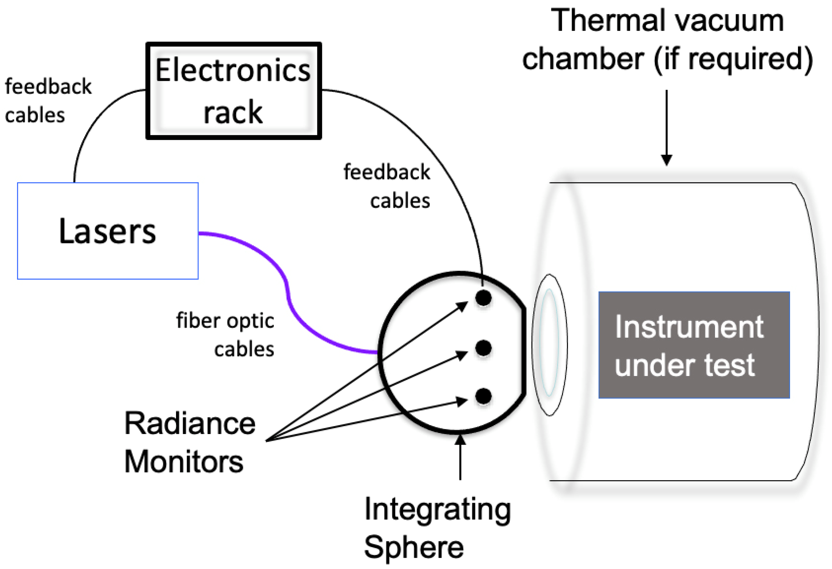
Remotesensing 16 00981 g001
Figure 2. Notional diagram of the GLAMR setup, which would illuminate either transfer radiometer or the instrument under test.
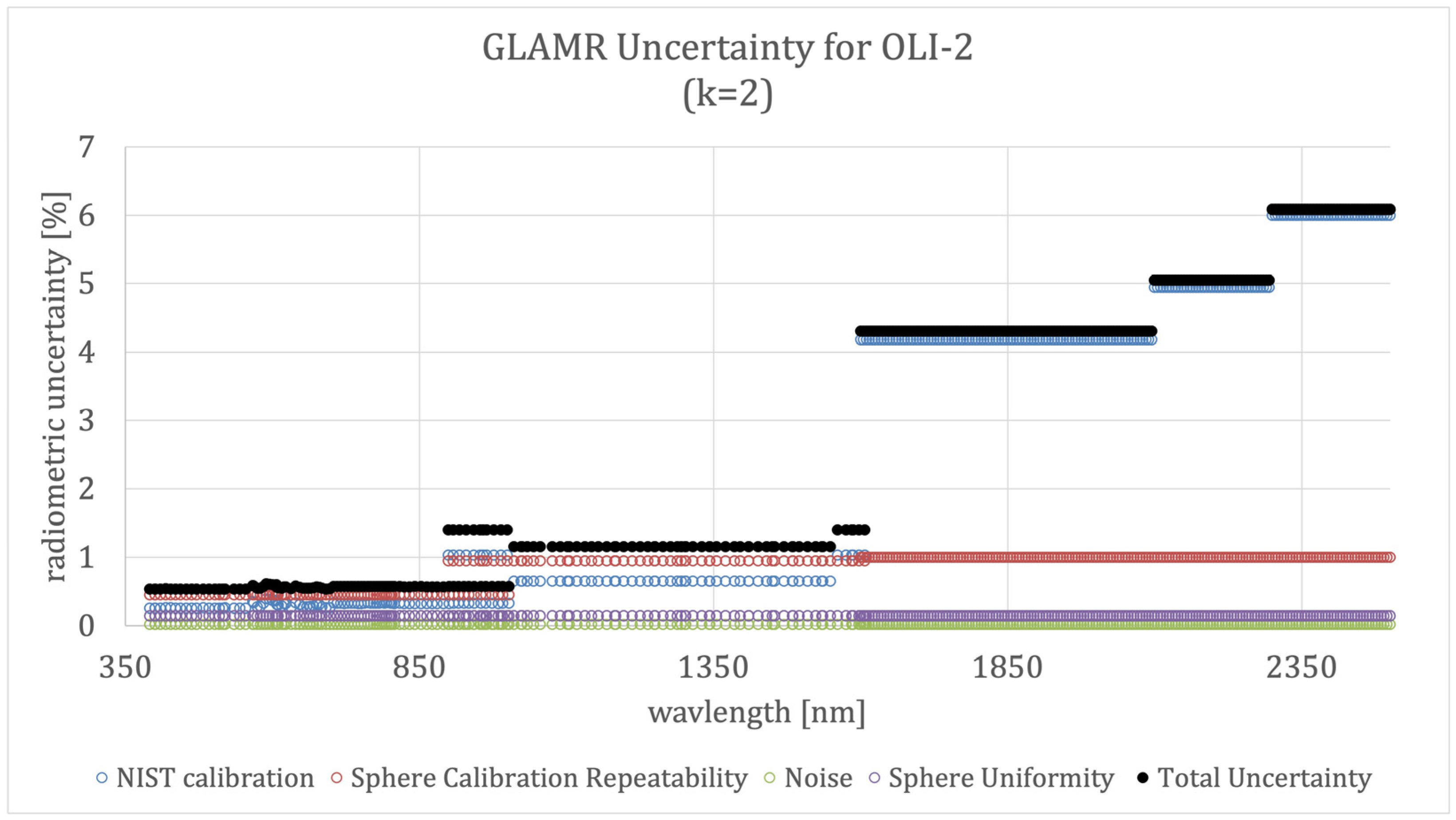
Remotesensing 16 00981 g002
Figure 3. The per-wavelength GLAMR Uncertainty budget. The largest uncertainties are from the NIST calibration of the transfer radiometers, though the uncertainty in the repeatability of the GLAMR calibration process is significant above 900 nm.
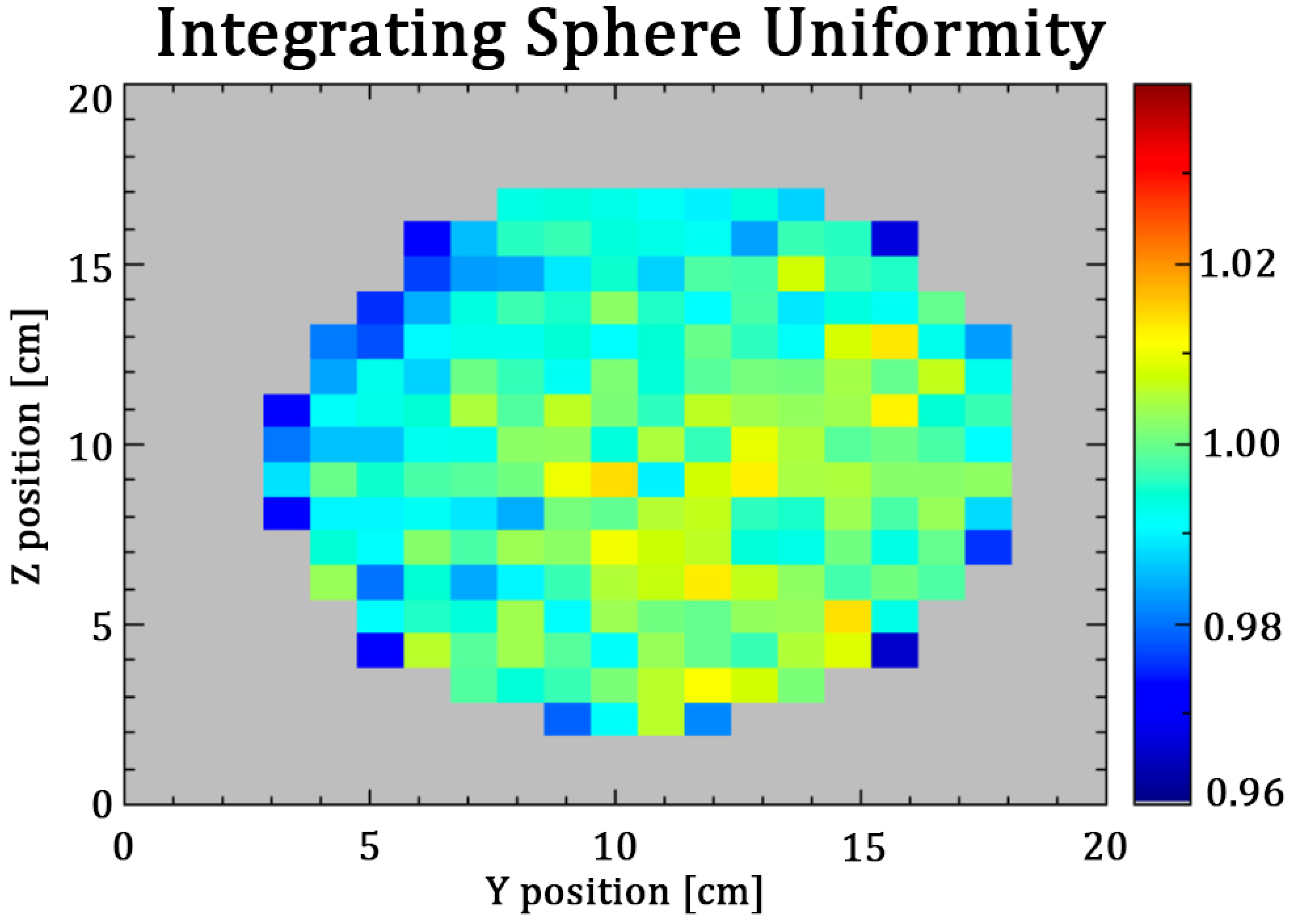
Remotesensing 16 00981 g003
Figure 4. Spatial variability map of the NIST spherical integrating source as measured by scanning a 1° field-of-view radiometer across the port in a 20 × 20 grid in 1 cm intervals. The plot shows the relative brightness of each location relative to the mean 5 × 5 grid in the center.
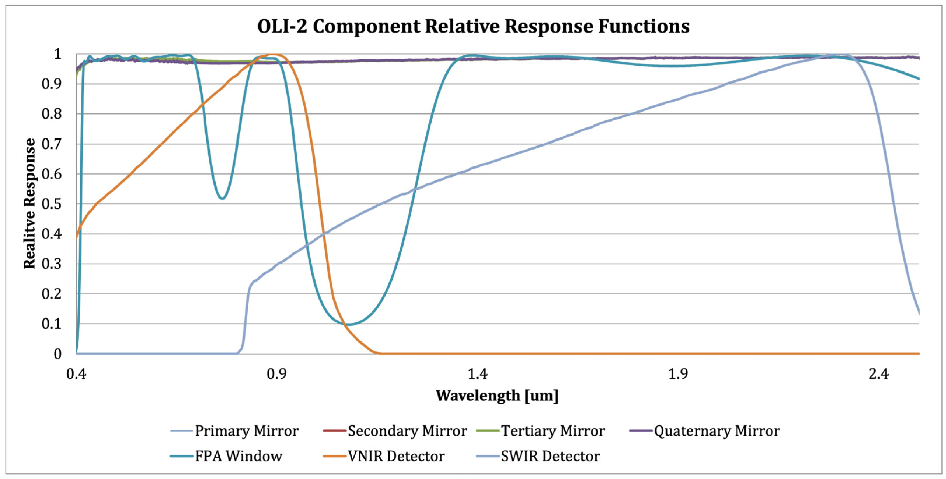
Remotesensing 16 00981 g004
Figure 5. Relative transmission or reflectance of the OLI-2 optical path components over the entire spectral range of the instrument, including some out-of-band response. Detector responses are radiance (power) based.
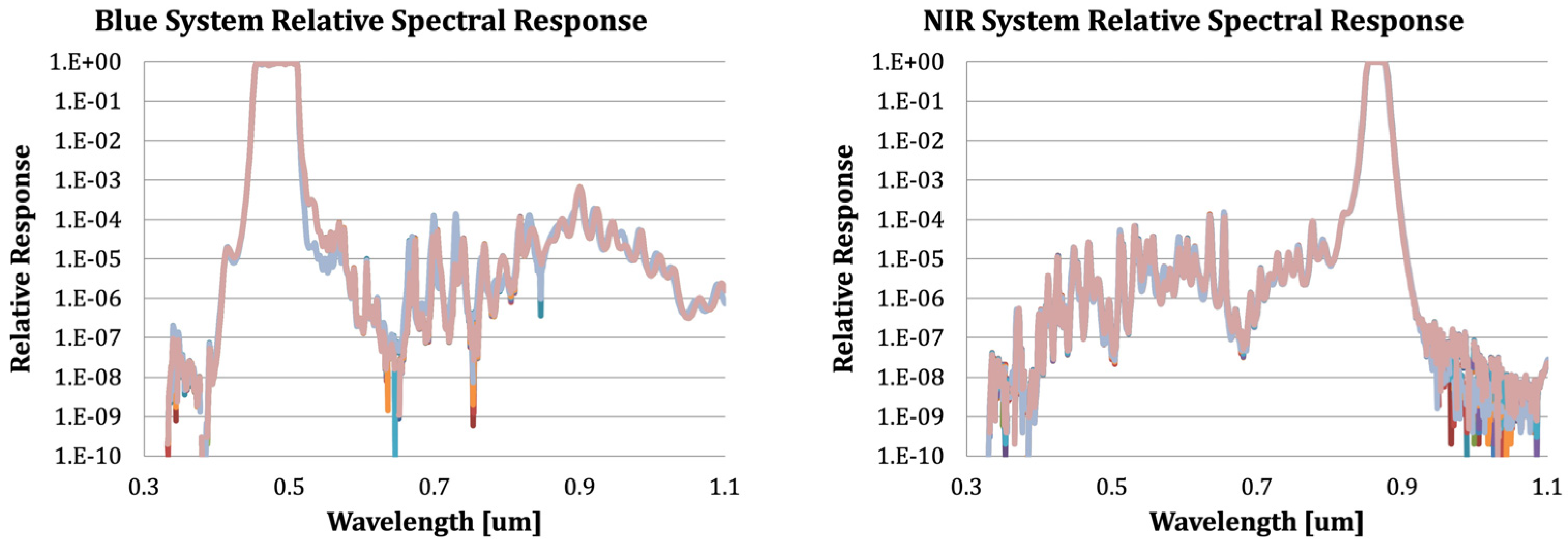
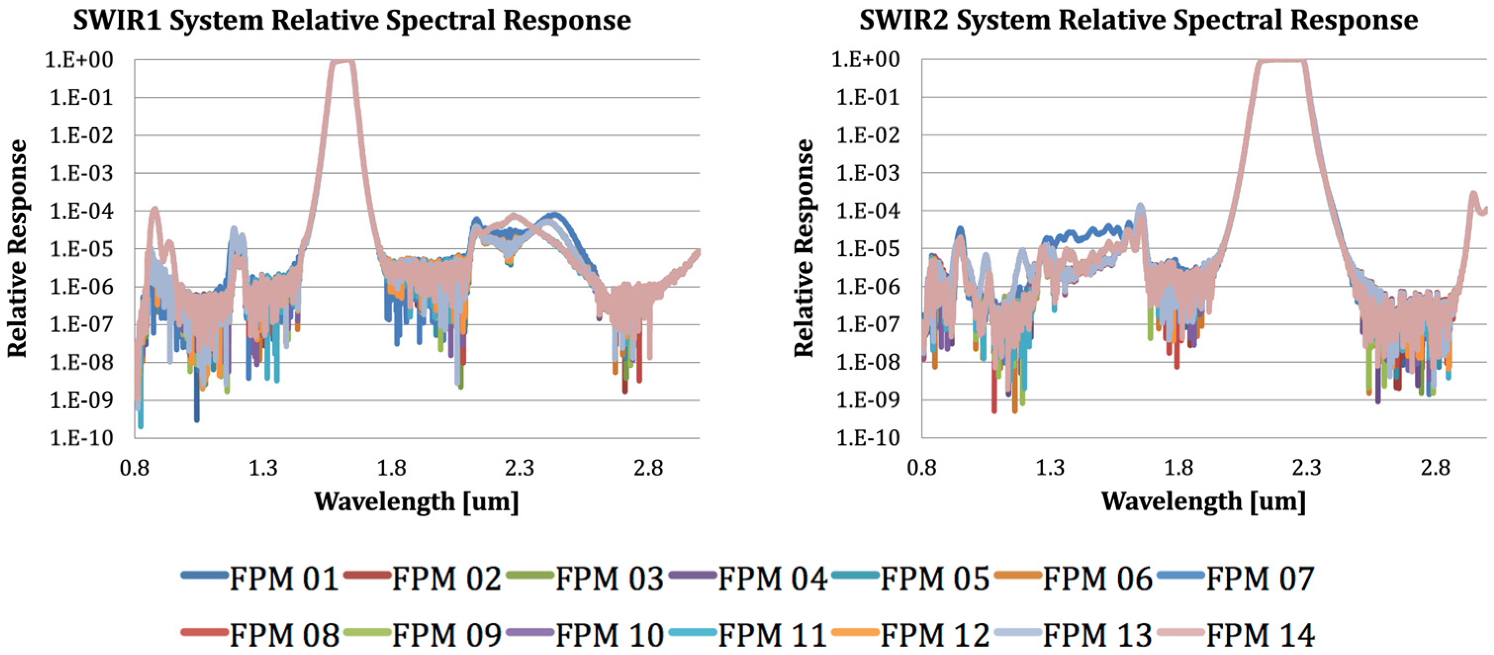
Remotesensing 16 00981 g005
Figure 6. System-level relative radiance spectral response functions estimated from component-level measurements for each FPM of the OLI-2 Blue, NIR, SWIR1, and SWIR2 bands, including out-of-band response. The out-of-band response is below 0.001 in all FPMs of all bands.
Remotesensing 16 00981 g006aRemotesensing 16 00981 g006b
Figure 7. The OLI-2 VNIR bands and SWIR band out-of-band response based on FPM-level measurements with optical components (mirrors and FPA window) included analytically. The plots are scaled to show the out-of-band response, so the in-band response is not shown here.
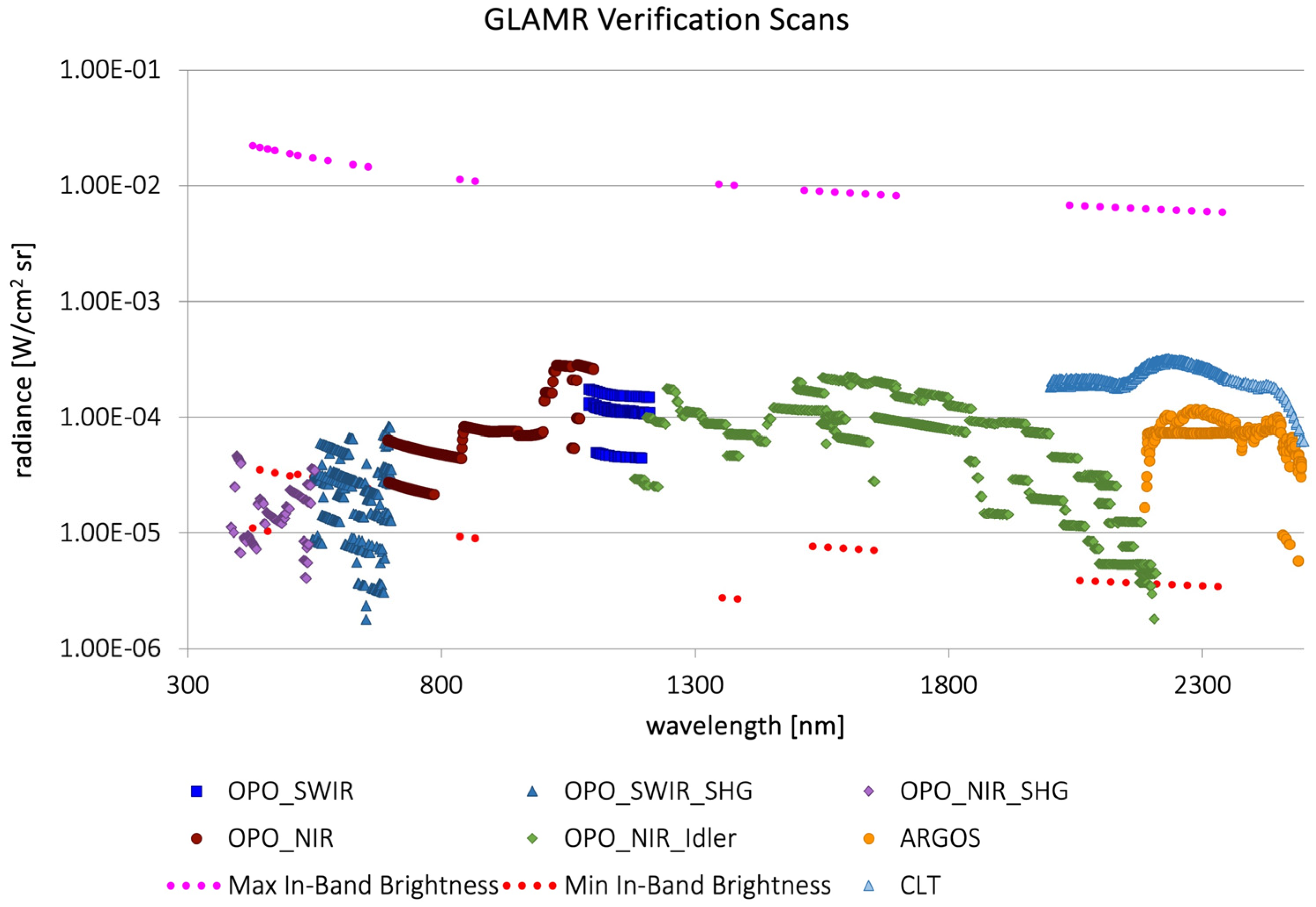
Remotesensing 16 00981 g007
Figure 8. The radiances generated by the GLAMR system for requirements verification in February 2018 at typical power levels across the full spectral range required for the test. The requirement radiances, maximum in-band radiances, and minimum in-band radiances are also shown. The GLAMR power can be reduced such that the maximum in-band radiance will not be exceeded, but in general, these data were acquired at the maximum power that could be expected. This means that there will be wavelengths below 700 nm where the minimum in-band radiance will not be met. The minimum out-of-band radiances, which are higher than the minimum in-band radiances, are not shown here, but were generally not met below 700 nm.
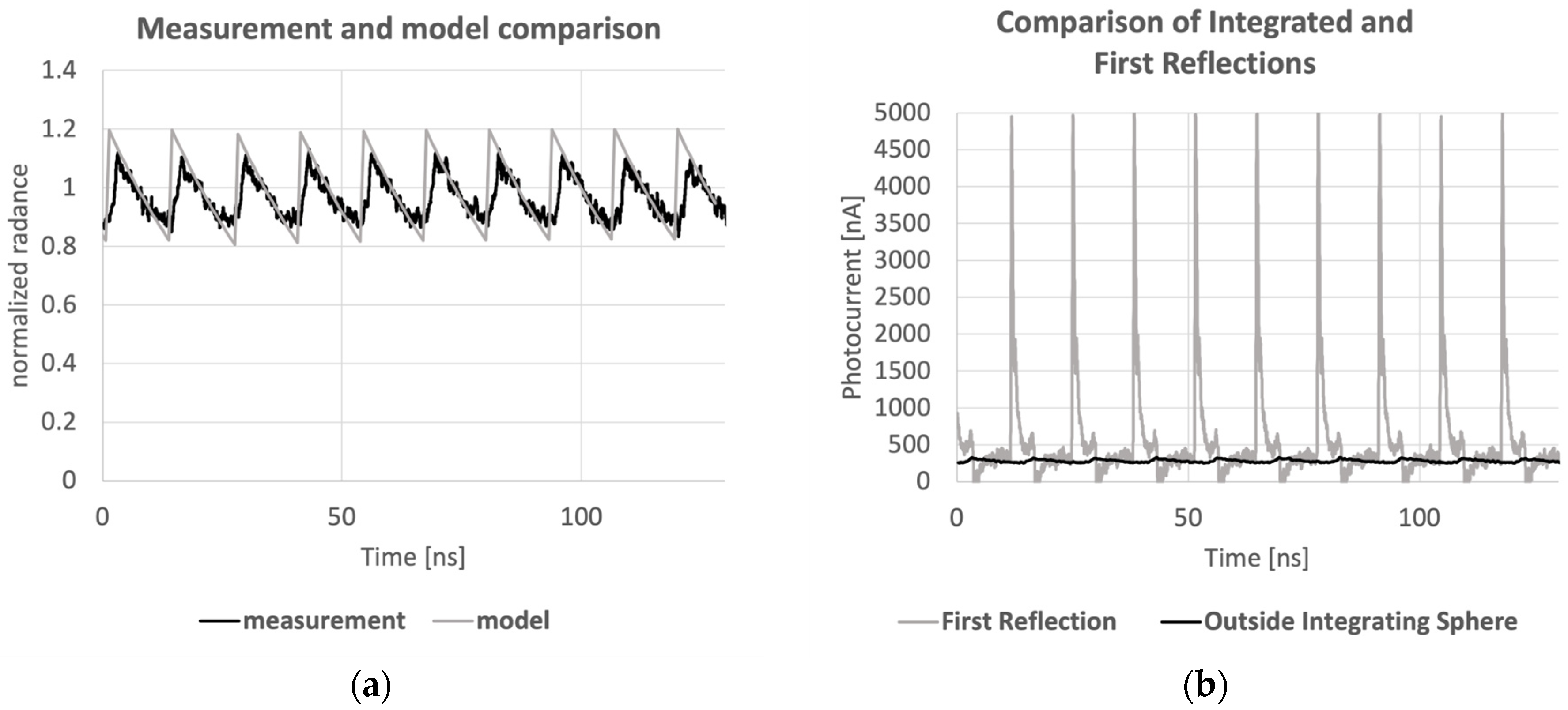
Remotesensing 16 00981 g008
Figure 9. (a) The results of the integrating sphere model radiance output after the limit cycle is met (grey) with measurements of radiance exiting the sphere (black). (b) The signal from outside the integrating sphere (black) and inside the sphere on the wall near the first reflectance (grey). The black lines are the same data in both plots.
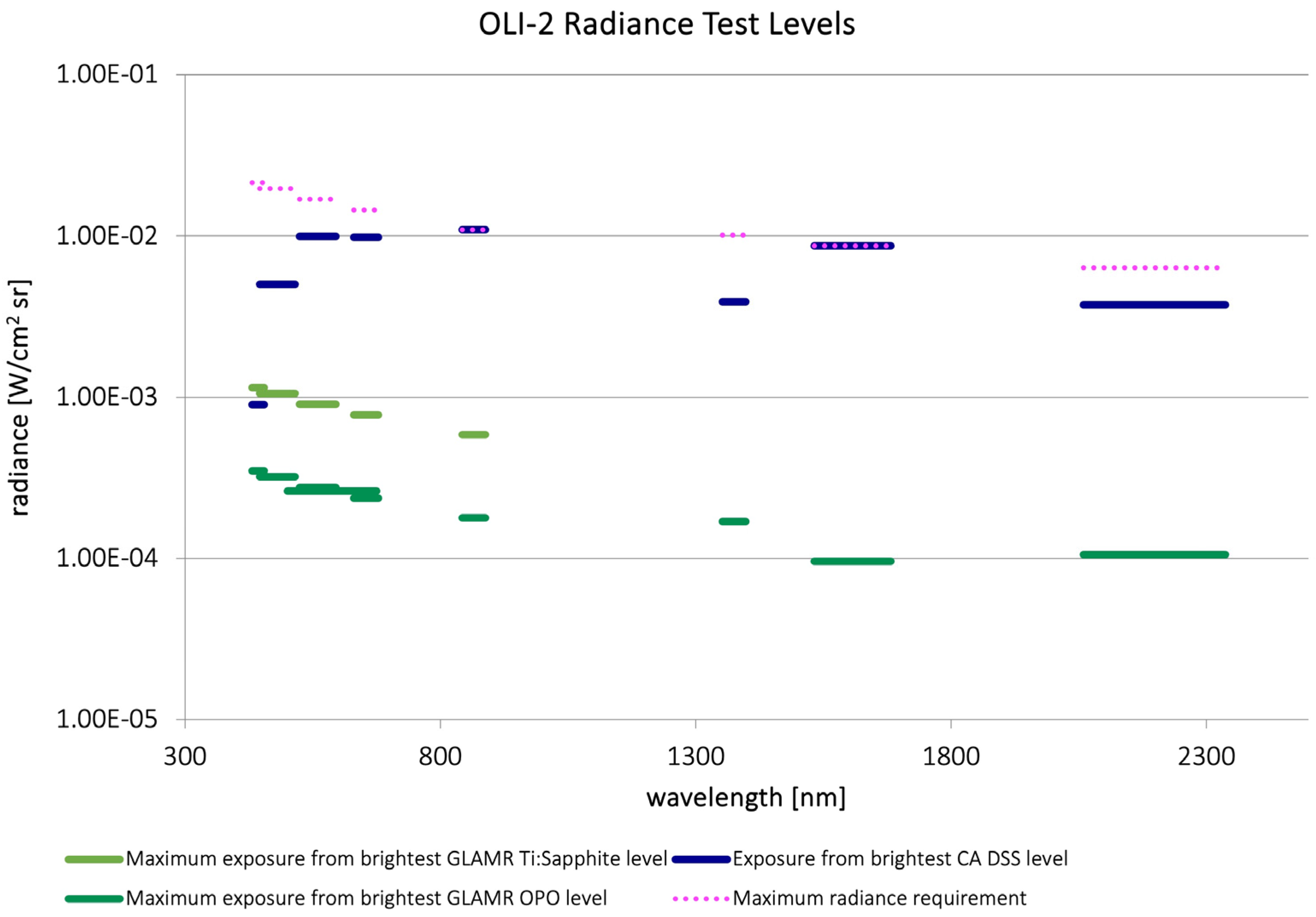
Remotesensing 16 00981 g009
Figure 10. OLI-2 specification radiances (dotted lines) and exposure radiances for the GLAMR risk assessment (solid lines). The maximum radiance that OLI-2 spare module was exposed to during the GLAMR damage study was an order of magnitude lower than the radiance from the brightest DSS lamp level.
Remotesensing 16 00981 g010
Figure 11. Per-detector responsivity of the NIR band as derived from exposure with the pulsed laser and the continuous wave laser, shown as relative to the mean from the continuous wave laser. The difference between them is about 1%, which is within the expected uncertainty of the measurements.
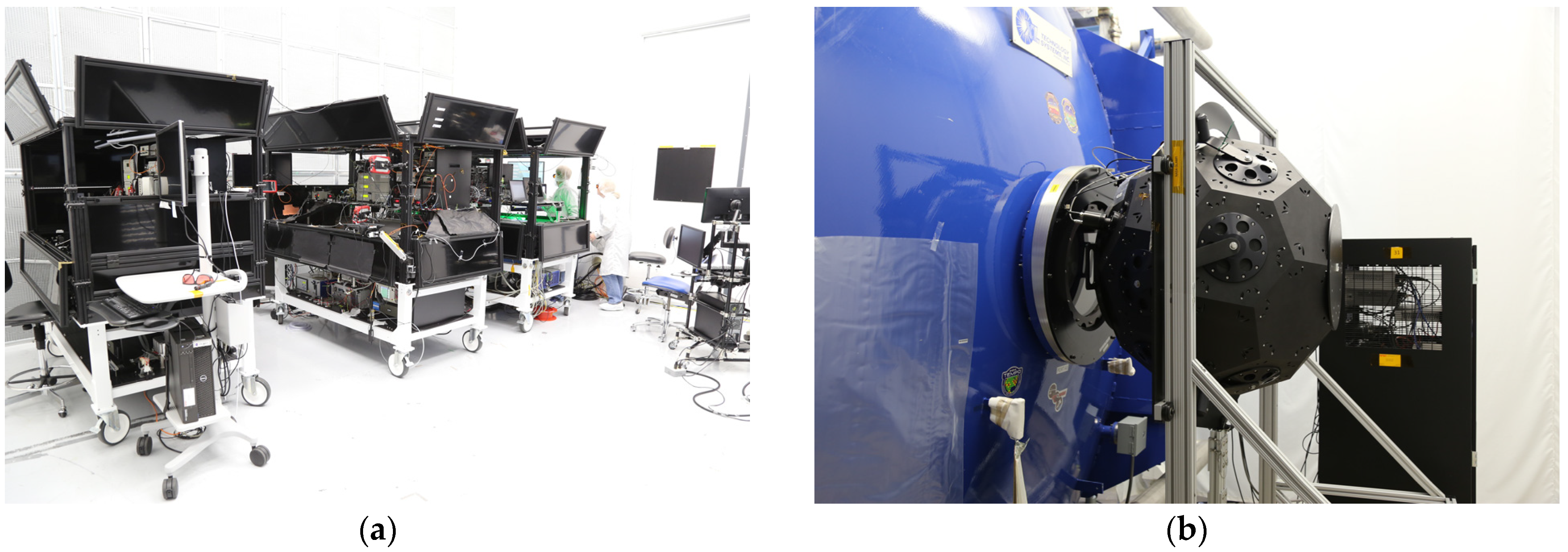
Remotesensing 16 00981 g011
Figure 12. The GLAMR set up at Ball. The three OLAF tables are located in a room adjacent to the TVAC chamber (a). The integrating sphere and the TVAC chamber are shown in (b), before the final alignment of the sphere to the chamber window/OLI-2. Once complete, the space between the chamber window and the sphere was covered with a light-tight shroud. The energy from the laser tables is coupled to the integrating sphere via fiber optic cables and feedback from the sphere monitor radiometers for stability control is returned to the tables via BNC cables.
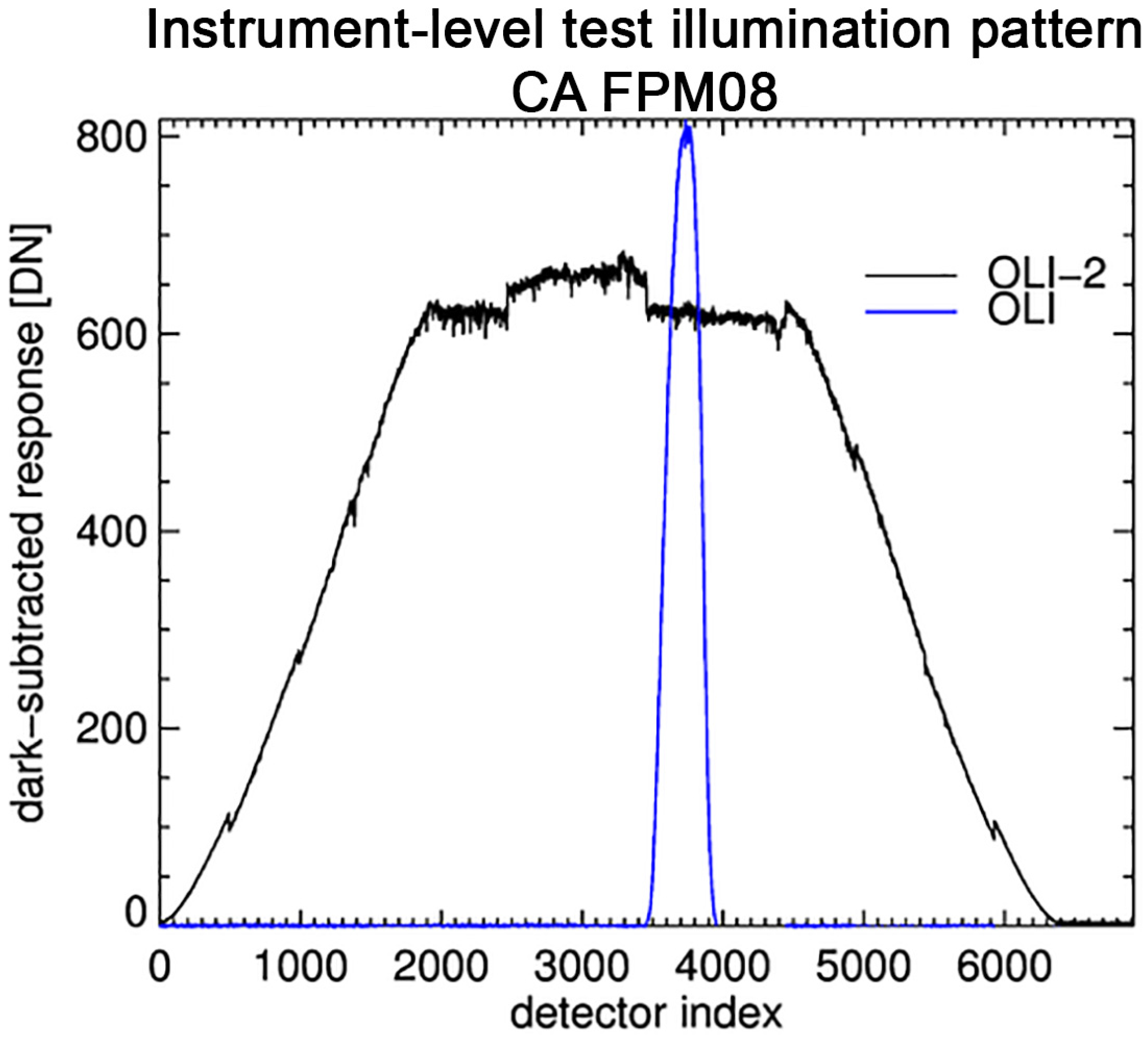
Remotesensing 16 00981 g012
Figure 13. Sample illumination pattern of the GLAMR sphere across the OLI-2 focal plane (black). Each module is 494 detectors wide and can be distinguished by discontinuities in the response. The sphere fully illuminates 5 of the 14 modules at once. For the instrument level test, the OLI-2 was rotated so that the sphere was centered on each of the modules at every wavelength. For reference, the blue line illustrates the spatial coverage of the monochromator used for the characterization of OLI. The spectral response was measured for about 14% of the detectors during the OLI test, as opposed to 100% of the detectors for OLI-2. Note that this plot is only intended to illustrate the difference in the illumination pattern, not the absolute signal levels.
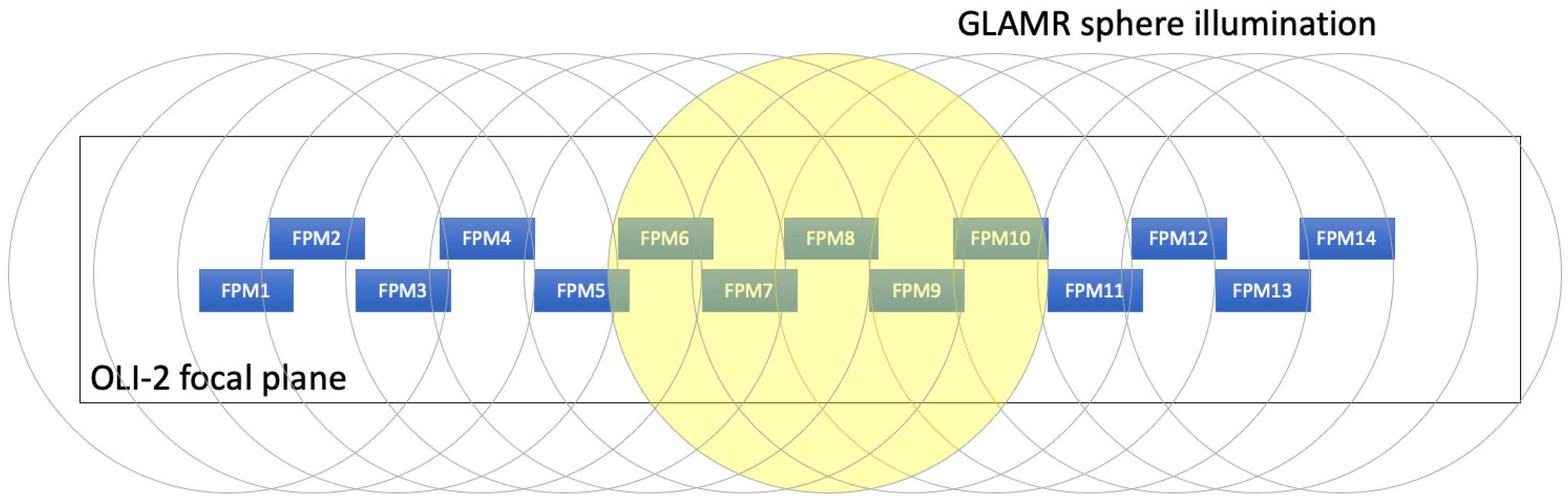
Remotesensing 16 00981 g013
Figure 14. Progression of the GLAMR illumination across the OLI-2 focal plane. Each circle represents the projection of the GLAMR sphere port on the focal plane, covering about five modules at once; one circle is yellow to clarify a single image’s coverage. Each wavelength measurement would begin with the GLAMR beam centered on either FPM1 or FPM14. The OLI-2 would capture a two-second image then rotate by about 1° to center on the next module. The process to capture images centered on every module for each wavelength took two minutes.
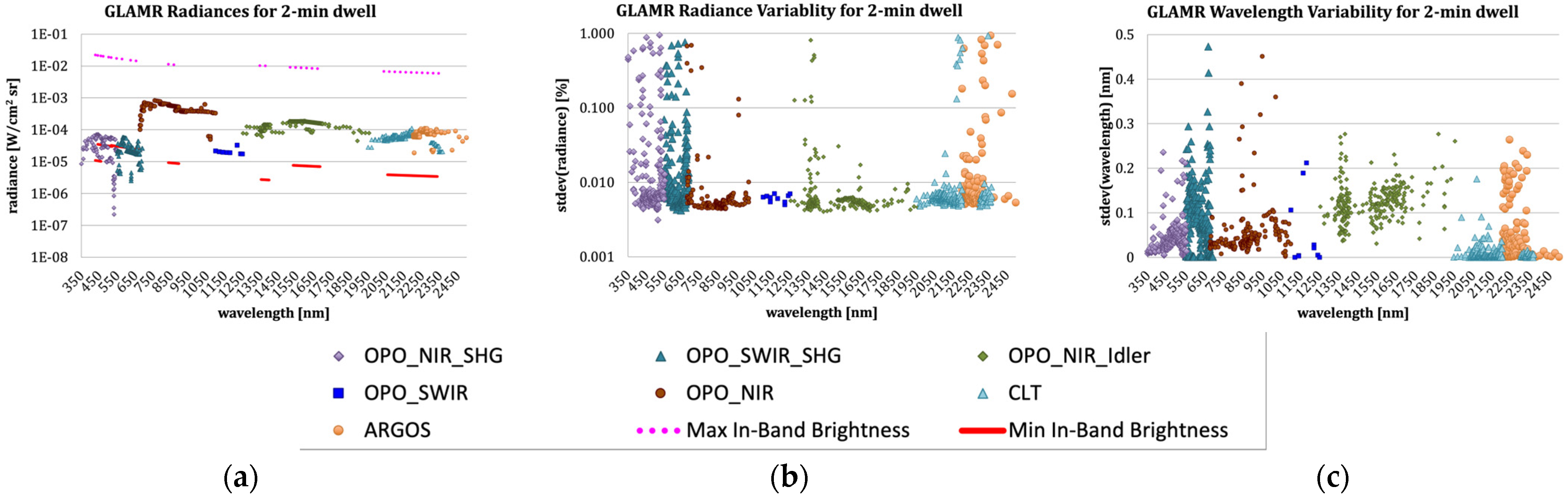
Remotesensing 16 00981 g014
Figure 15. The GLAMR signal (a) and radiometric (b) and spectral (c) stability over the two minutes that OLI-2 was capturing images. In (a), the radiance level achieved for every valid measurement shown and is compared to the maximum and minimum requirement radiances. The radiances below 700 nm are close to the minimum or below. Note that these data have been screened for 1% radiometric stability over 2 min, but only data with 0.01% radiometric stability or better over the 2 s of each OLI-2 image acquisition were used for generation of the RSR.
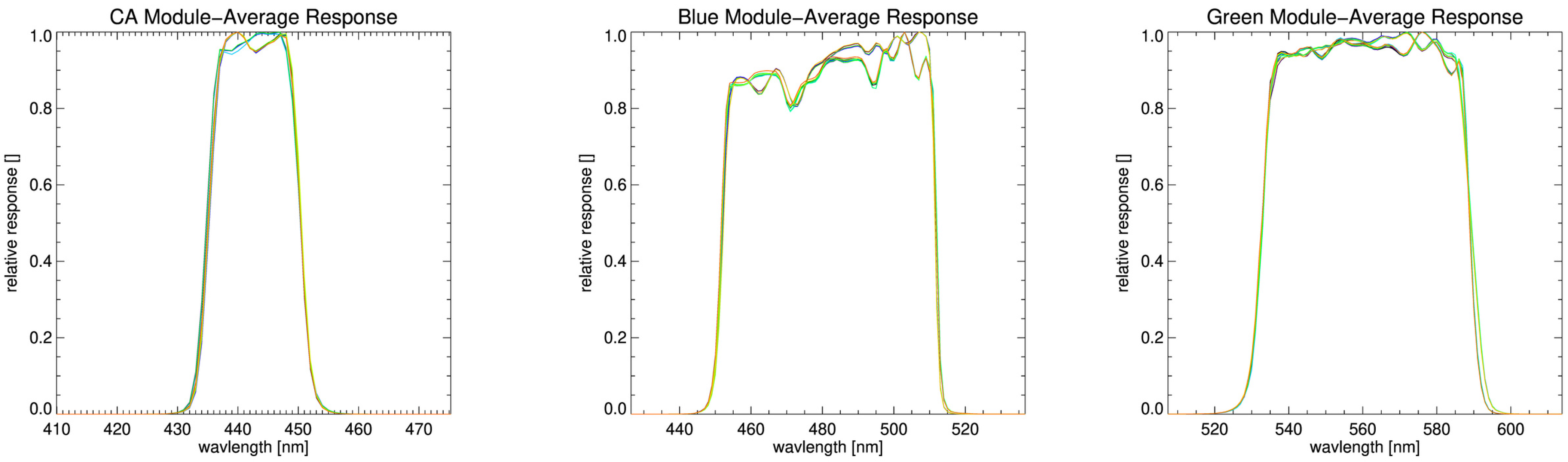
Remotesensing 16 00981 g015
Figure 16. The module-average in-band relative spectral response of all nine OLI-2 spectral bands as measured by GLAMR. Each module is represented by a different color.
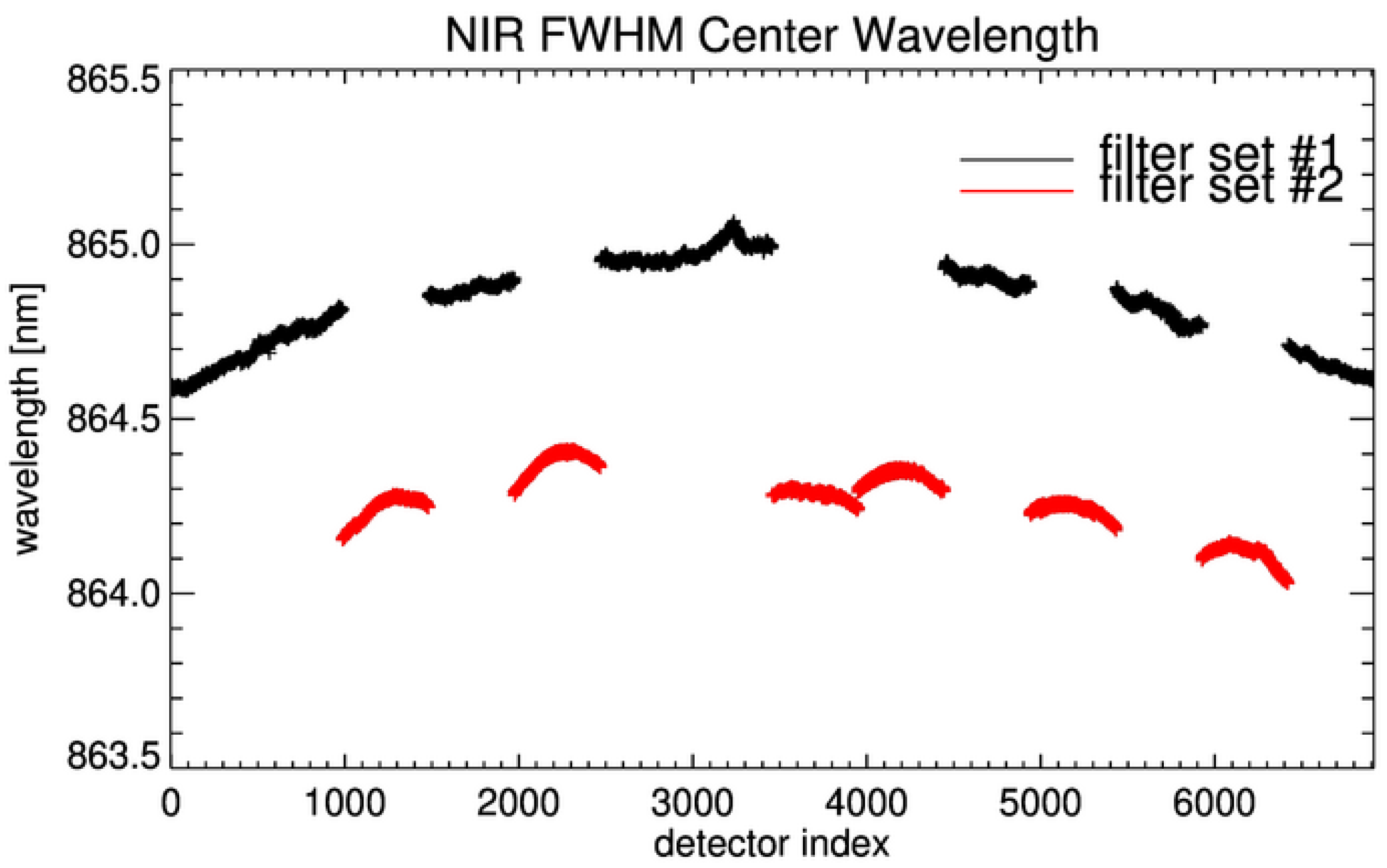
Remotesensing 16 00981 g016aRemotesensing 16 00981 g016b
Figure 17. The per-detector center wavelength across the focal plane for the NIR band. Differences are the result of filter wafer source and the change in angle-of-incidence. The red and black series distinguish between modules built with common filter sources and the offset between the two is expected. The overall frown shape across the focal plane is the result of the angle-of-incidence and is also expected.
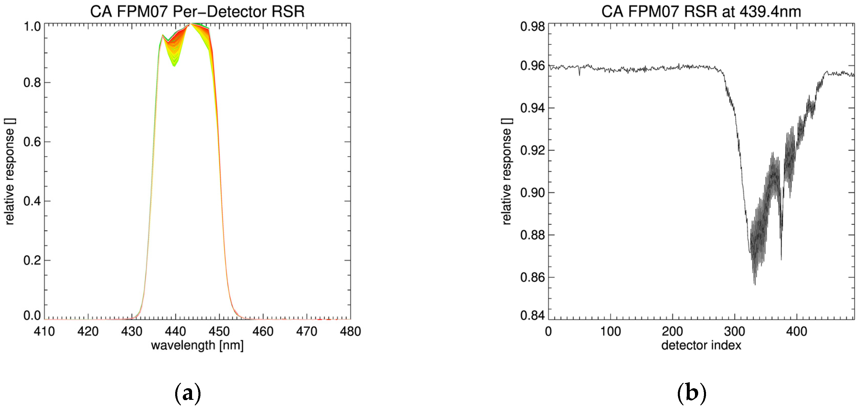
Remotesensing 16 00981 g017
Figure 18. The per-detector RSR for the CA band FPM07 (a), where each detector’s response is a different color, and the response at 439.4 nm across every detector (b). The variation in the response between 435 and 445 nm is apparent in (a). About 170 detectors are affected by what is likely an imperfection in the filter, where the response drops from about 0.955 to as low as 0.86 (b).
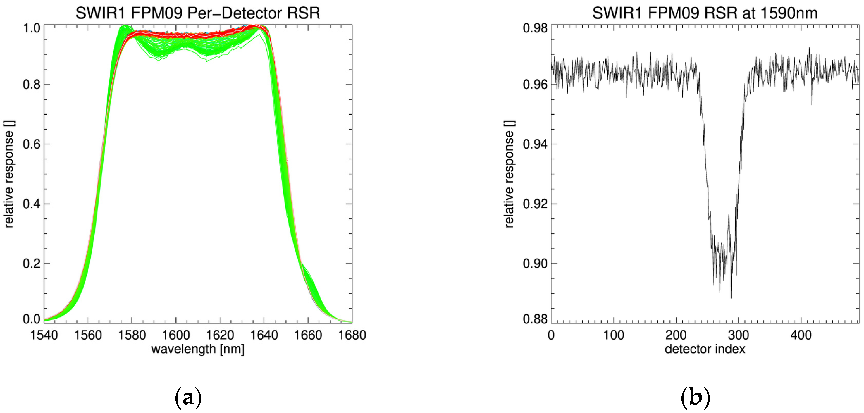
Remotesensing 16 00981 g018
Figure 19. The per-detector RSR for the SWIR1 band FPM09 (a), where each detector’s response is a different color, and the response at 1590 nm across every detector (b). The variation in the response across the high response region is apparent in (a). About 100 detectors are affected by what is likely an imperfection in the filter, where the response drops from about 0.965 to as low as 0.89 (b).
Remotesensing 16 00981 g019
Figure 20. The per-detector RSR for the Blue band FPM13 (a), where each detector’s response is a different color, and the bandwidth at the 50% response points for every detector in FPM13 (b). The variation in the response across the high response region and the lower band edge are apparent in (a). About 70 detectors are affected by what is likely an imperfection in the filter, where the bandwidth narrows by up to 1 nm (b).
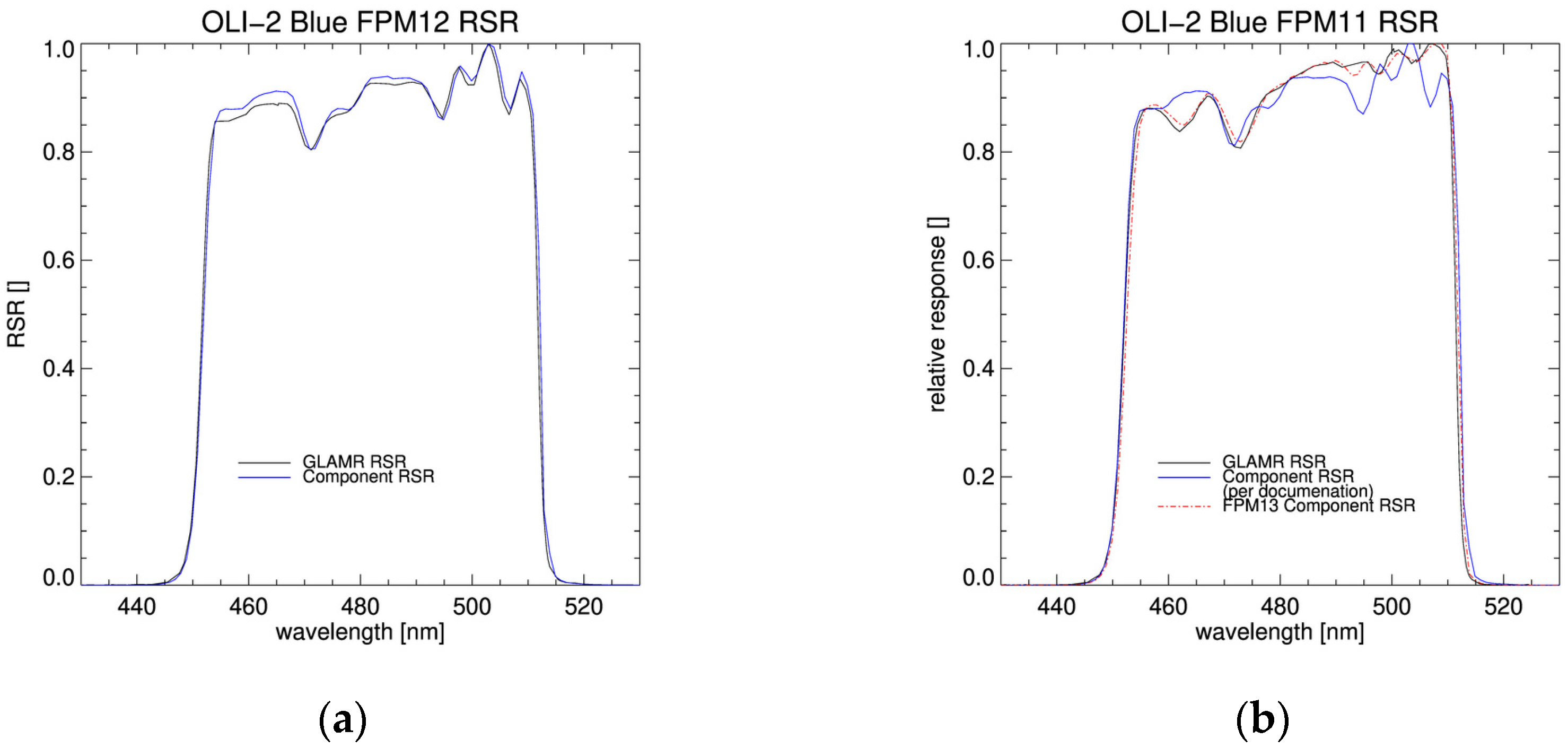
Remotesensing 16 00981 g020
Figure 21. The module-average relative spectral response for two OLI-2 modules in the Blue band at the instrument-level and as predicted from the component-level measurements. The GLAMR results match the component-level prediction very well for FPM12 (a), but there are significant differences in the features in FPM11 (b). There were two different wafers used as the source of the Blue band filter sticks; it is likely that the filter stick used on FPM11 originated from the other wafer. The FPM13 component-level RSR is shown on (b) to illustrate the better match with the other wafer. Table 2 reflects this discovery.
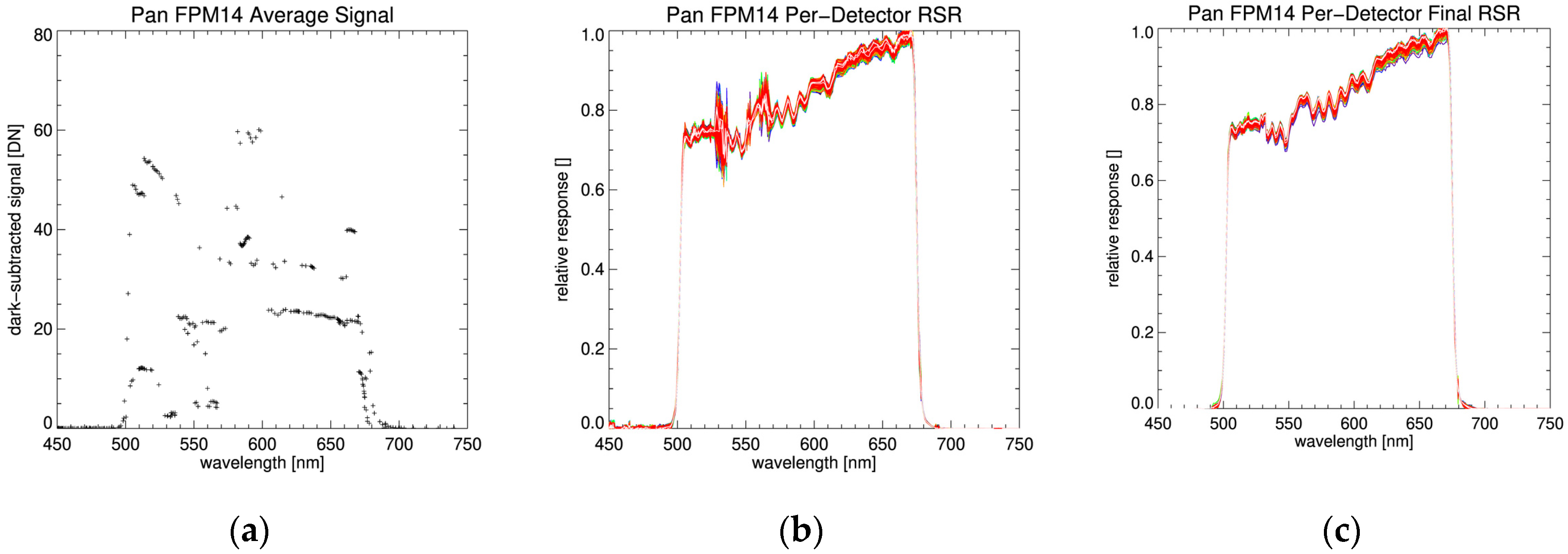
Remotesensing 16 00981 g021
Figure 22. The OLI-2 average signal level for one module of the Pan band (a). Low signal levels in the degeneracy region of the OPO (~532 nm) and where the efficiency of two OPO configurations are falling off (between 550 and 570 nm) result in noisy RSR at those wavelengths, as illustrated in (b) of the RSR for all 988 detectors on the module, where each detector’s response is represented by a different color. In (c), the per-detector RSR with the low-signal regions are smoothed to better represent instrument response rather than noise.
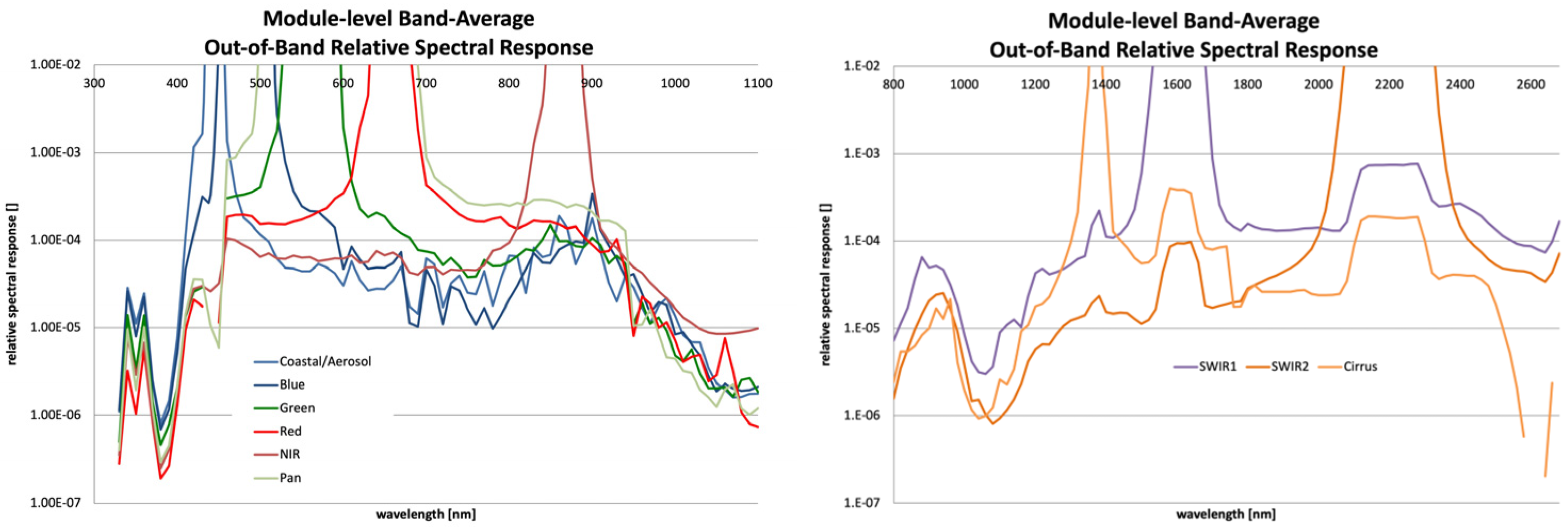
Remotesensing 16 00981 g022
Figure 23. The module-average relative spectral response for all 14 OLI-2 module in each band. Each module is a different color. Due to the lack of power in below ~700 nm, the GLAMR measurements were not used for final assessment of out-of-band response in the VNIR bands. All three SWIR bands exhibit some amount of cross-talk, which was expected based on OLI results.
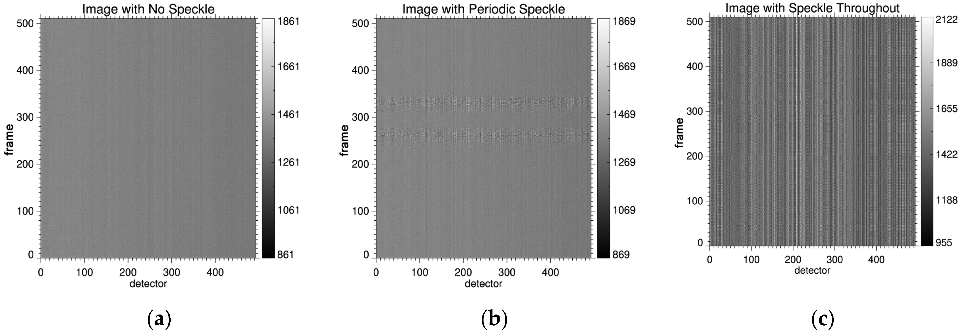
Remotesensing 16 00981 g023
Figure 24. The effect of speckle on the OLI-2 imagery. In (a), the image was acquired with no speckle; the fiber was being vibrated for the duration of the image. In (b), the image was acquired while the fiber was being vibrated, but the vibrations stopped for two very short periods, apparent at about line 275 and 325. In (c), the image was acquired without the fiber being vibrated, and the impact is apparent in the non-uniformity across the detectors. Speckle increases the noise across the detectors from about 1.5% to about 9%. The images are all scaled to about 1000 counts to aid in the visibility of the different noise levels.
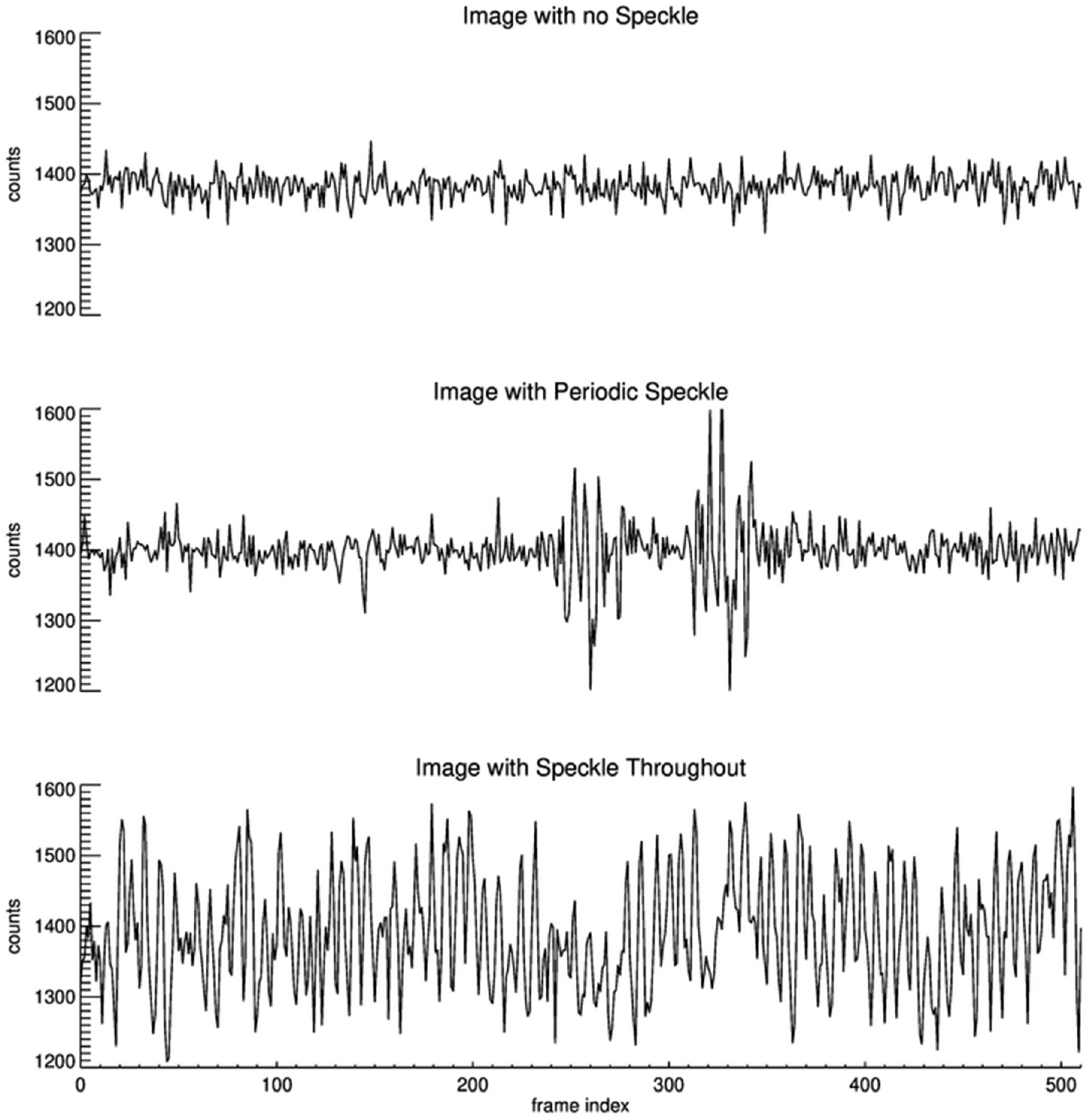
Remotesensing 16 00981 g024
Figure 25. Plots of signal over time for the first detector in each image shown in Figure 24. When there is no speckle, the typical signal varies by less than 1.5%. With speckle, the typical signal varies by 6%.
Remotesensing 16 00981 g025
Figure 26. Top-of-atmosphere radiances for two surface types to be used in OLI-2 simulations. These are the same targets used for OLI simulation.
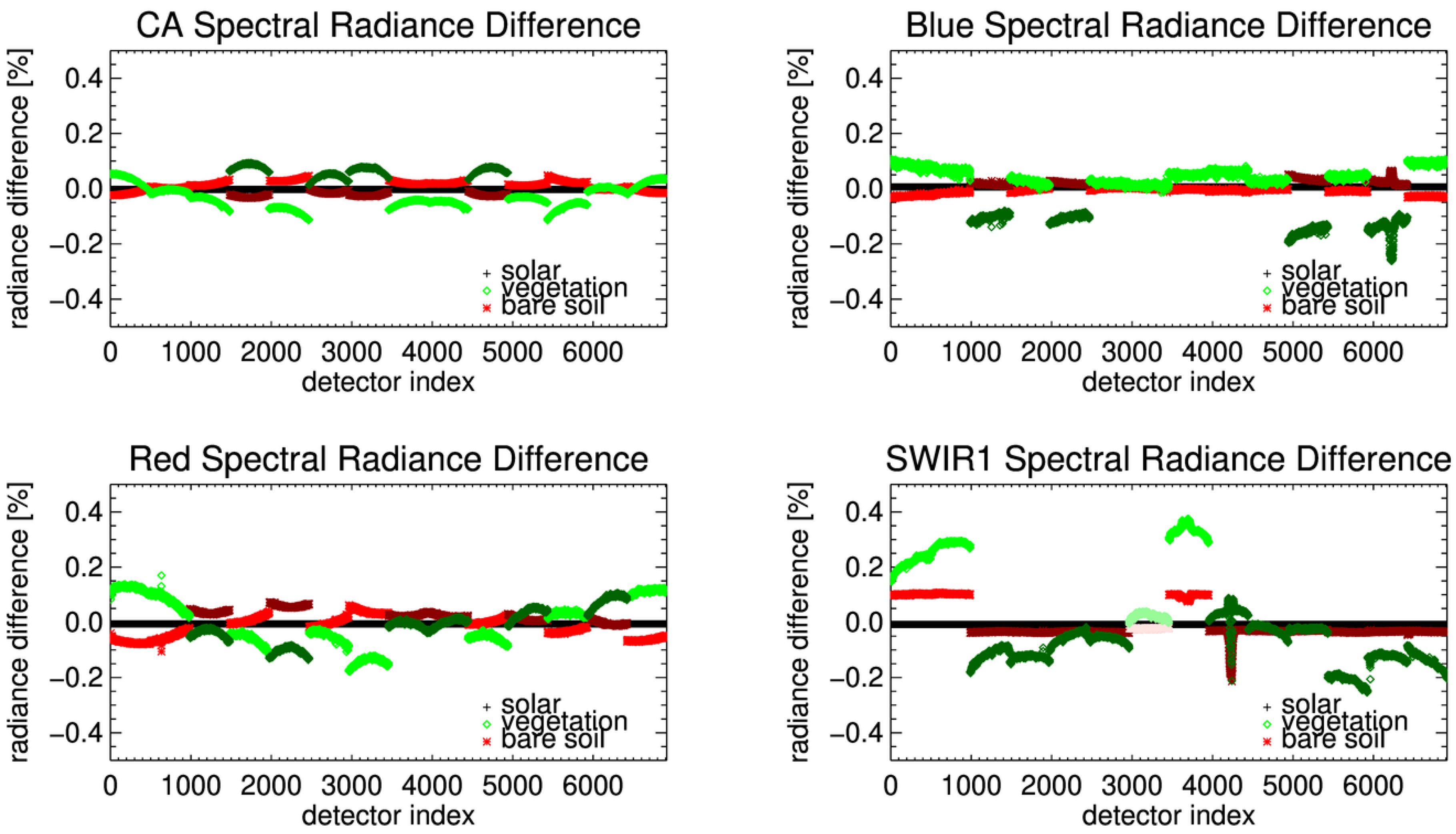
Remotesensing 16 00981 g026
Figure 27. The spectral radiance difference across the focal plane for the standard target types as a result of per-detector differences in the RSR and the lack of telecentricity in the telescope. The shades of red and green represent the different source filter across the focal plane (see Table 2). The largest discontinuities are the result of spectral mismatches at the edges of modules. Internal to each module, the differences are generally very small except for modules where features were discovered in the filter material (i.e., SWIR1 FPM09).
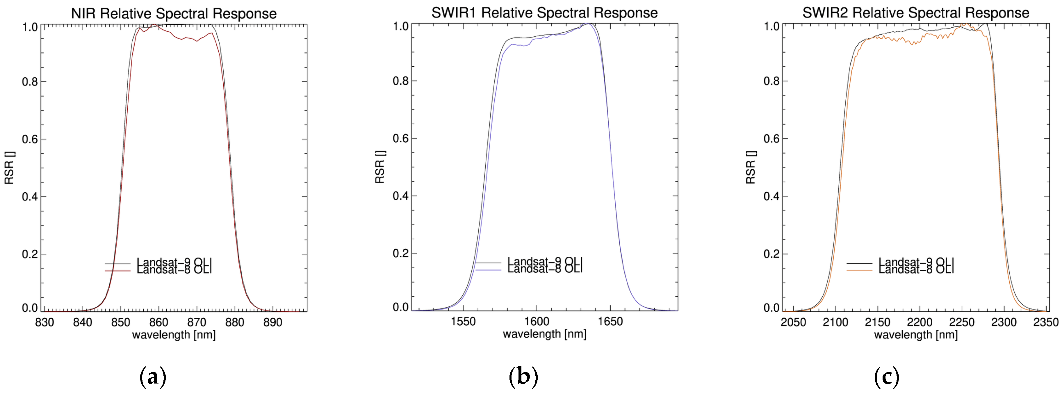
Remotesensing 16 00981 g027
Figure 28. A comparison of the OLI-2 and OLI band-average RSR for sample bands.
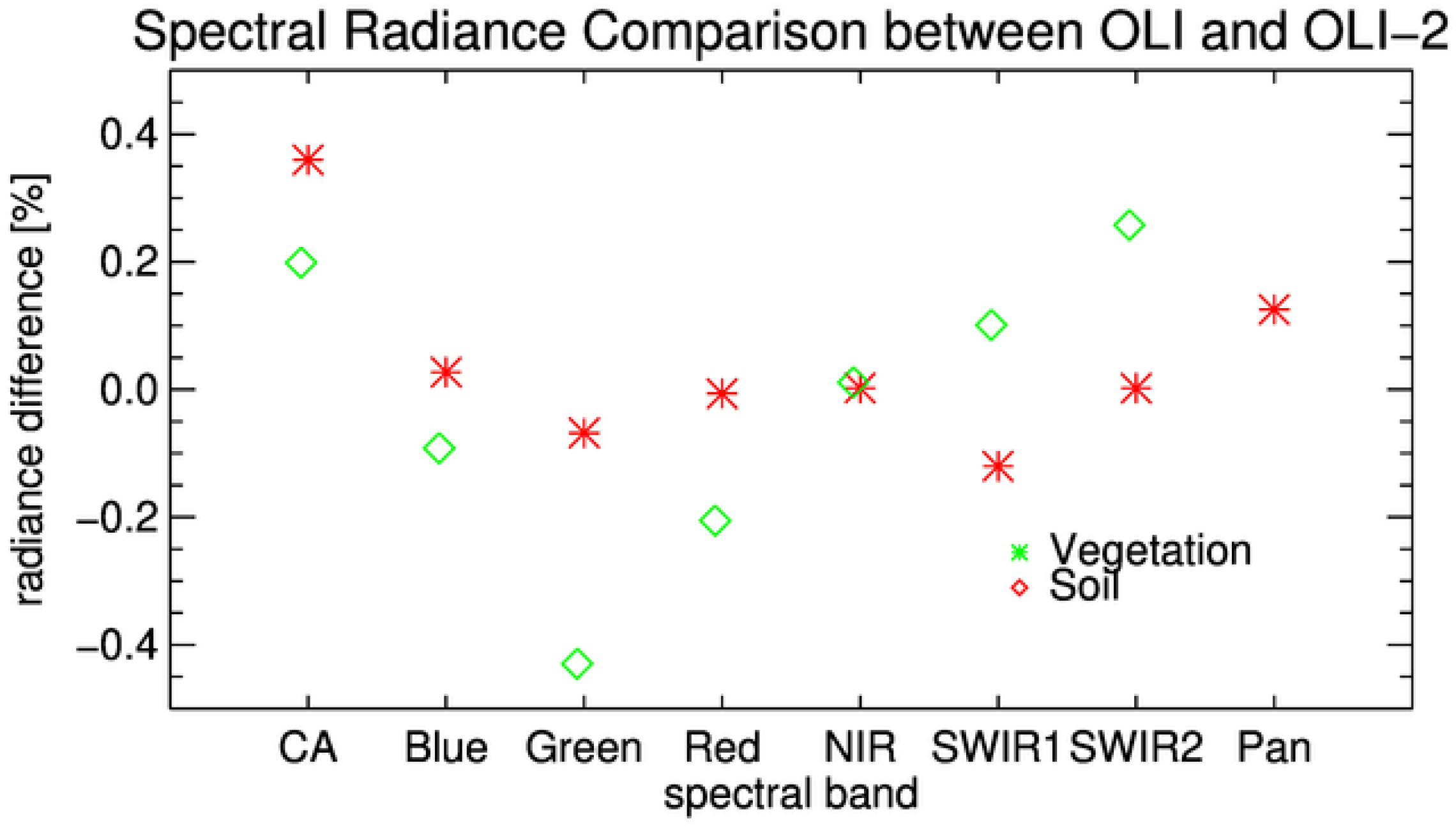
Remotesensing 16 00981 g028
Figure 29. The comparison of the integrated spectral radiance for OLI-2 and OLI band-average RSR. For these target types, the radiances agree within 0.5% based strictly on the relative spectral response, except for the Pan band vegetation radiance, which is off the scale of this plot at 1.45% different.
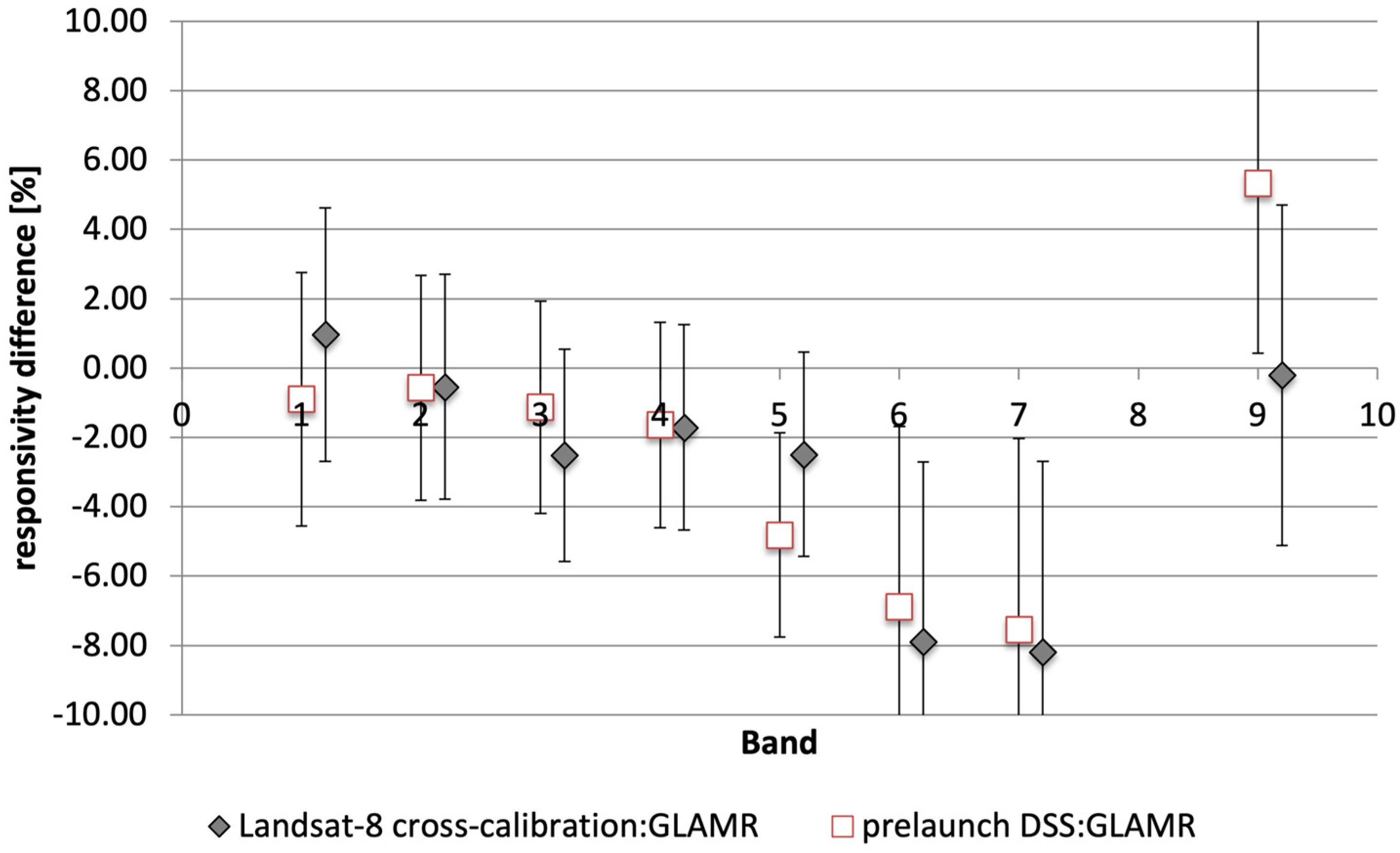
Remotesensing 16 00981 g029
Figure 30. Comparison of DSS-derived OLI-2 responsivities and GLAMR derived responsivities. The error bars are the RSS of the DSS radiometric uncertainty and the GLAMR radiometric uncertainty.
Remotesensing 16 00981 g030
Table 1. Landsat-9 OLI-2 spectral bands, as defined by the requirements. The upper and lower band edges are defined at the 50% response point and the center wavelength is the mid-point between edges.
Spectral BandSpatial
Resolution [m]
Minimum Lower Band Edge [nm]Maximum Upper Band Edge [nm]Center
Wavelength [nm]
Coastal/Aerosol (CA)30433453443 ± 2
Blue30450515482 ± 5
Green30525600562 ± 5
Red30630680655 ± 5
NIR30845885865 ± 5
SWIR130156016601610 ± 10
SWIR230210023002200 ± 10
Pan15500680590 ± 10
Cirrus30136013901375 ± 5
Table 2. Filter wafer distribution across the OLI-2 focal plane. Numbers indicate which wafer was the source of the filter for each module (colors are to aid in visibility). Italicized numbers indicate that filter sticks from that wafer were also used on the OLI focal plane. Unlike for OLI, no band consists of filters from only one wafter source. SWIR1 and SWIR2 have filters from three different source wafers. The wafer numbers are indexed continuously from the OLI build, so can be compared to the OLI table in [1].
FPM NumberCA Blue Green Red NIR Cirrus SWIR1 SWIR2 Pan
1323334434
2323334434
3312214333
4423335344
5312214333
6423335344
7423335254
8322214433
9322215343
10423334334
11312215343
12323334334
13312214333
14323335344
Table 3. GLAMR laser configuration and spectral coverage used for OLI-2 characterization.
Laser ConfigurationSpectral RangePulse Repetition Frequency
OPO_NIR_SHG350–550 nm76 or 80 MHz Pulsed
OPO_SWIR_SHG550–700 nm76 or 80 MHz Pulsed
OPO_NIR700–1100 nm76 or 80 MHz Pulsed
OPO_SWIR1100–1350 nm76 or 80 MHz Pulsed
OPO_NIR_Idler1350–2200 nm76 or 80 MHz Pulsed
CLT1900–2500 nmContinuous wave
ARGOS2200–2500 nmContinuous wave
Table 4. Total GLAMR uncertainty for each of the OLI-2 spectral bands.
Spectral BandCenter Wavelength [nm]GLAMR Total
Uncertainty (k = 2) [%]
CA443 ± 20.5
Blue482 ± 50.5
Green562 ± 50.5
Red655 ± 50.5
NIR865 ± 50.6
SWIR11610 ± 104.3
SWIR22200 ± 104.3
Pan590 ± 100.6
Cirrus1375 ± 51.2
Table 5. A sample of the Ball Aerospace requirements on the GLAMR system.
SpecificationRequirementVerification Method
Spectral RangeGLAMR shall operate in a spectral range of 425–2350 nm (with a goal range of 350–2500 nm) with gaps allowed between 700–830 nm, 900–1340 nm, 1410–1520 nmTest
In-band wavelength step sizeThe wavelength scan step size of the source shall be equal to 1 nm for VNIR and Cirrus bands and 2 nm for SWIR1, SWIR2, and PAN bandsTest
Wavelength resolution (full-width half maximum)The FWHM spectral bandpass shall be ≤1 nm for VNIR and Cirrus and ≤2 nm for SWIR1, SWIR2, and PAN bandsDemonstrated with measurements and wavemeter specifications
Out-of-band wavelength step sizeThe wavelength scan step size of the source shall be equal to 10 nm below 1 µm and 20 nm above 1 µmTest
Test source sizeThe GLAMR source shall illuminate the FPA unvignetted over a FOV more than 1 degree in-track by +/−1.5 degrees cross-trackAnalysis: Code V GLAMR/OLI-2 optical system analysis (Ball internal report)
In-band source brightnessGLAMR shall be capable of outputting radiance levels greater than specified values over the given wavelength rangesTest (Figure 8)
Out-of-band source brightnessGLAMR should be capable of outputting radiance levels greater than specified values over the given wavelength rangesTest, but generally struggled to meet the requirement below 700 nm
Source Maximum brightnessGLAMR shall not exceed the maximum radiance levels specified values over the given wavelength rangesTest (Figure 8)
Source Radiance Monitor
Characterization
The calibration accuracy of the GLAMR source radiance monitor shall be <2% from 400 nm to 1600 nm and <5% from 1600 nm to 2500 nm.Analysis (Figure 3, Table 4)
StabilityGLAMR radiance output shall remain stable for a minimum of 2 min for all bands except PAN; minimum of 4 min for PAN. Stability is defined as a standard deviation of ≤0.01% over a 30 s average of the sphere monitor dataDemonstration
Table 6. Sampling specifications for the GLAMR instrument-level test of OLI-2. The linewidth provided is an estimate of what is typical for the spectral range. It may be dependent on laser configuration. The out-of-band regions are considered to be those wavelengths not covered by any spectral band. The Pan region listed below is only those wavelengths which were not covered by the in-band sampling in the other VNIR bands.
Spectral BandSpectral Range [nm]GLAMR Step Size [nm]GLAMR Nominal Linewidth [nm]
CA, Blue,
Green, Red
428–68410.1
NIR836–89410.1
Cirrus1346–140410.15
SWIR11514–169820.15
SWIR22038–236520.2 with CLT
1.1 with ARGOS
Pan600–63020.1
Out-of-band350–430,
680–840,
890–1100
100.1
Out-of-band1100–1350,
1404–1514,
1690–2050,
2365–2495
200.15 with OPO
0.2 with CLT
1.1 with ARGOS
Table 7. Variability in center wavelength across each band. Means and standard deviations are provided for the whole band. The center wavelength mean is provided for the average of all detectors in each filter set to illustrate the differences due to spectral filter mismatch in the filter lots. SWIR1 and SWIR2 are the only spectral bands that use a filter from the third set of wafers (per Table 2). These filter sets are numbered arbitrarily and do not link to the numbering in Table 2.
Spectral BandCenter Wavelength,
All Modules
Center Wavelength, Filter Set 1Center Wavelength, Filter Set 2Center Wavelength, Filter Set 3
Mean [nm]Standard Deviation [nm]Mean [nm]Mean [nm]Mean [nm]
CA442.720.12442.79442.55
Blue481.740.07481.73481.77
Green560.770.12560.71560.85
Red654.240.17654.22654.25
NIR864.570.30864.84864.27
SWIR11607.930.351608.371607.781607.89
SWIR22199.590.412199.592199.642199.91
Pan588.810.13588.79588.76
Cirrus1374.090.211374.111374.08
Table 8. The maximum and average variation of radiance within the worst-case module for each band. The largest variation is seen for vegetation, generally across the filters with the imperfections. The Cirrus Band is not included in this analysis because the signal in this band is so weak.
Spectral BandMaximum VariationAverage Variation
Vegetation [%]Soil [%]Vegetation [%]Soil [%]
CA0.020.010.010.00
Blue0.030.010.010.00
Green0.030.010.020.01
Red0.030.020.010.01
NIR0.000.000.000.00
SWIR10.030.040.020.00
SWIR20.010.020.010.01
Pan0.030.010.020.01
Table 9. The maximum and average radiance differences between adjacent modules across the focal plane, along with the RMS variability due to the spectral response differences for sample targets calculated using a band-average RSR. The vegetation discontinuities are larger than the soil, likely due to the fact that the soil is more spectrally similar to the solar spectra and solar data are used to flat-field the results. The Cirrus Band is not included in this analysis because the signal in this band is so weak.
Spectral BandMaximum DiscontinuityAverage DiscontinuityRMS Variability
Vegetation [%]Soil [%]Vegetation [%]Soil [%]Vegetation [%]Soil [%]
CA0.160.060.070.030.090.03
Blue0.240.060.120.020.140.03
Green0.240.010.170.010.180.01
Red0.140.090.060.040.070.04
NIR0.080.010.050.010.050.01
SWIR10.400.140.120.030.180.06
SWIR20.160.070.060.030.080.04
Pan0.250.030.160.010.180.02
Table 10. The band-average summaries of OLI and OLI-2 as determined from the instrument-level spectral characterization.
Spectral BandOLIOLI-2
Band Width [nm]Lower Band Edge [nm]Upper Band Edge [nm]Center Wavelength [nm]Band Width [nm]Lower Band Edge [nm]Upper Band Edge [nm]Center Wavelength [nm]
CA15.98434.97450.95442.9615.51435.06450.57442.81
Blue60.04452.02512.06482.0459.87451.96511.82481.89
Green57.33532.74590.07561.4156.50532.71589.20560.95
Red37.47635.85673.32654.5936.88635.88672.76654.32
NIR28.25850.54878.79864.6728.77850.26879.03864.64
SWIR184.721566.501651.221608.8686.151565.081651.221608.15
SWIR2186.662107.402294.062200.73189.482105.382294.862200.12
Pan172.40503.30675.70589.5020.901363.681384.571374.13
Cirrus20.391363.241383.631373.43172.47503.09675.56589.32
Table 11. Band-average responsivities as derived from the GLAMR test and from the DSS test. The analysis was not performed on the Pan band.
Spectral BandDSS Band-Average Responsivity
[counts/W/m2 sr μm]
GLAMR Band-Average Responsivity
[counts/W/m2 sr μm]
Responsivity Difference [%]GLAMR
Uncertainty [%] (k = 2)
OLI-2
Uncertainty [%] (k = 2)
CA16.1164215.97351−0.890.53.62
Blue18.9522118.84482−0.570.53.2
Green19.5497119.33102−1.130.53.02
Red19.3686519.05563−1.640.52.92
NIR31.6136330.16167−4.810.52.9
SWIR1167.16763156.41167−6.8843.3
SWIR2544.07684507.02169−7.3143.78
Cirrus88.4781793.465565.34 11.24.7
1 The Cirrus band DSS-derived responsivity provided here was used as the at-launch radiometric gain. It was determined after launch that it had been derived incorrectly, so although the difference between the DSS and GLAMR responsivities are large, the difference has been revised downwards (see [25]).
Table 12. Band-average responsivities as derived from the GLAMR test and from the cross-calibration with Landsat-8. The analysis was not performed on the Pan band.
Spectral BandLandsat-8 Cross-Calibration Band-Average Responsivity
[counts/W/m2 sr μm]
GLAMR Band-Average Responsivity
[counts/W/m2 sr μm]
Responsivity Difference [%]GLAMR
Uncertainty [%] (k = 2)
OLI-2
Uncertainty [%] (k = 2)
CA15.8193315.973510.970.53.62
Blue18.9465318.84482−0.540.53.2
Green19.8167819.33102−2.510.53.02
Red19.3824719.05563−1.720.52.92
NIR30.9121530.16167−2.490.52.9
SWIR1168.75106156.41167−7.8943.3
SWIR2547.38303507.02169−7.9643.78
Cirrus93.6574393.46556−0.211.24.7
Disclaimer/Publisher’s Note: The statements, opinions and data contained in all publications are solely those of the individual author(s) and contributor(s) and not of MDPI and/or the editor(s). MDPI and/or the editor(s) disclaim responsibility for any injury to people or property resulting from any ideas, methods, instructions or products referred to in the content.

