MVP-Stereo: A Parallel Multi-View Patchmatch Stereo Method with Dilation Matching for Photogrammetric Application

Abstract

Multi-view stereo plays an important role in 3D reconstruction but suffers from low reconstruction efficiency and has difficulties reconstructing areas with low or repeated textures. To address this, we propose MVP-Stereo, a novel multi-view parallel patchmatch stereo method. MVP-Stereo employs two key techniques. First, MVP-Stereo utilizes multi-view dilated ZNCC to handle low texture and repeated texture by dynamically adjusting the matching window size based on image variance and using a portion of pixels to calculate matching costs without increasing computational complexity. Second, MVP-Stereo leverages multi-scale parallel patchmatch to reconstruct the depth map for each image in a highly efficient manner, which is implemented by CUDA with random initialization, multi-scale parallel spatial propagation, random refinement, and the coarse-to-fine strategy. Experiments on the Strecha dataset, the ETH3D benchmark, and the UAV dataset demonstrate that MVP-Stereo can achieve competitive reconstruction quality compared to state-of-the-art methods with the highest reconstruction efficiency. For example, MVP-Stereo outperforms COLMAP in reconstruction quality by around $30\%$ of reconstruction time, and achieves around $90\%$ of the quality of ACMMP and SD-MVS in only around $20\%$ of the time. In summary, MVP-Stereo can efficiently reconstruct high-quality point clouds and meet the requirements of several photogrammetric applications, such as emergency relief, infrastructure inspection, and environmental monitoring.

1. Introduction

Three dimensional reconstruction based on RGB images is more convenient and less costly compared to RGB-D sensors and lasers, and has a very wide range of applications in various industries [1,2,3], laying the foundation for 3D perception [4,5,6,7,8]. Generally, the 3D reconstruction pipeline includes structure from motion (SfM) [9,10], multi-view stereo (MVS) [11,12,13,14,15,16,17], mesh reconstruction [18,19,20,21,22] and texture mapping [23], where MVS tries to obtain correspondence between pixels on images to reconstruct a dense 3D point cloud. With the rapid development of sensors, such as the charge-coupled device (CCD) and the complementary metal oxide semiconductor (CMOS), and delivery platforms, such as the mobile phone and the unmanned aerial vehicle (UAV), the quality and quantity of images have been greatly improved, making it an urgent need to improve the reconstruction efficiency of MVS while maintaining the reconstruction quality.

A large amount of MVS methods have been proposed in the field of computer vision [15,16,17] and photogrammetry [1,11,12,13,14]. Based on the image features used for pixel matching, MVS methods can be divided into traditional methods and learning-based methods. Traditional methods use handcrafted features for pixel matching, while learning-based methods leverage high-level semantic features captured by a convolutional neural network (CNN) or Transformer.

1.1. Traditional MVS Methods

Traditional MVS methods can be classified into four categories [24,25,26], including voxel-based methods, surface evolution methods, patch-based methods, and depth map fusion methods. Voxel-based methods [27,28] split the space into several voxels and classify these voxels to estimate the 3D shape. Surface evolution methods [29,30] refine a rough surface via photometric consistency to reconstruct a high-quality surface. Patch-based methods [31,32,33,34] first detect feature points from texture-rich regions and gradually propagate depth information to neighboring pixels to obtain dense point cloud. However, these methods suffer from computation complexity and cannot be directly applied to large-scale scenes.

Depth map fusion methods are the dominant pipeline of MVS [15,16,17,31,35,36,37,38], which simplifies MVS to stereo matching by first estimating depth maps for each view and then fusing multiple depth maps to reconstruct dense point cloud [15,39]. Compared with other MVS methods, depth map fusion methods can directly work on large scenes and are easier for parallel compute depth maps for each image [15]. A straightforward idea is utilizing stereo matching methods to reconstruct disparity maps from each pair after stereo rectification, where the matching problem decreases to a one-dimensional search problem. SGM [40] is one of the most popular stereo matching methods [26], which builds a two-dimensional cost volume to determine disparity through locally aggregated costs. Following SGM, Rothermel et al. [35] improves the reconstruction efficiency of SGM via a coarse-to-fine strategy to narrow disparity search ranges at higher resolutions, and Hernandez-Juarez et al. [41] implements SGM on an embedded graphics processing unit (GPU) device to reliably produce disparity in real-time. Furthermore, Li et al. [36] utilizes a guided median filter post-processing step to refine the disparity generated by SGM, and Kuhn et al. [42] tries to model the uncertainty of disparity maps obtained from SGM to produce high-quality point clouds. However, stereo matching methods are not suitable for MVS, as they need to perform several stereo rectifications for each image, which has several neighbor images, and estimate disparity maps for each pair separately without benefiting from multi-view constrain.

Considering limitations of stereo matching methods, researchers extend patchmatch stereo [43] from stereo matching to multi-view stereo, which reconstructs the disparity map by random searching and spatial propagation without using the two-dimensional cost volume. Compared to SGM-based methods, patchmatch stereo does not need to build a two-dimensional cost volume for each pixel, and it is more friendly for high-resolution images and large scenes. Cernea [44] and Shen [15] first extend patchmatch stereo to MVS and determine the depth of each pixel by calculating photometric consistency via homography [45]. Zheng et al. [46] and Schönberger et al. [47] incorporate pixel-level view selection with depth estimation through a probabilistic framework. To improve the reconstruction efficiency, Galliani et al. [16] utilizes a red–black board to implement the patchmatch stereo, which parallelly operates half of all pixels in an image on a consumer-grade GPU. Then, Xu and Tao [37] employs an adaptive red–black board to parallelly propagate depth and pixel visibility and deals with low-texture regions by the multi-scale geometric consistency guidance through a coarse-to-fine strategy. To improve the reconstruction quality of low-texture regions, Kuhn et al. [48], and Romanoni and Matteucci [49] utilize superpixels to improve the completeness of the depth map through plane-fitting on superpixel regions. Xu et al. [50] uses the sparse feature points from SfM to initialize the depth map and further propagate planes with the related 2D image patch with less ambiguity. Meanwhile, Wang et al. [51] utilizes the mesh reconstructed on coarse images to guide the reconstruction of the high-resolution images. Xu et al. [38] assumes low-texture areas are piecewise planar and introduces plane priors through triangulating sparse reliable points in the 2D image domain. Stathopoulou et al. [52] uses plane priors guided by quadtree structures to enhance the propagation of more reliable depth estimates. Yuan et al. [53] relies on the Segment Anything Model to distinguish semantic instances in scenes and enhance the matching cost and the propagation in patchmatch to deal with texture-less regions. However, these methods struggle to balance reconstruction quality with reconstruction efficiency.

1.2. Learning-Based MVS Methods

The development of deep learning has brought new ideas to MVS, where CNN [54] or Transformer [55] can find robust semantic features. Yao et al. [54] proposes MVSNet, which firstly extracts the visual features from an image using a CNN, and then partitions the 3D space into a series of parallel planes based on the given depth range to construct a 3D matching cost volume by differential homography, and finally regresses the depth map by the 3D convolution. Following MVSNet, a large number of deep learning methods have emerged in recent years [56,57,58,59,60,61,62,63]. However, learning-based methods require a large amount of data to train the network and suffer from low generalization abilities on unseen scenes. Moreover, learning-based methods cannot directly deal with high-resolution images because of high GPU memory consumption [64].

1.3. Our Contributions

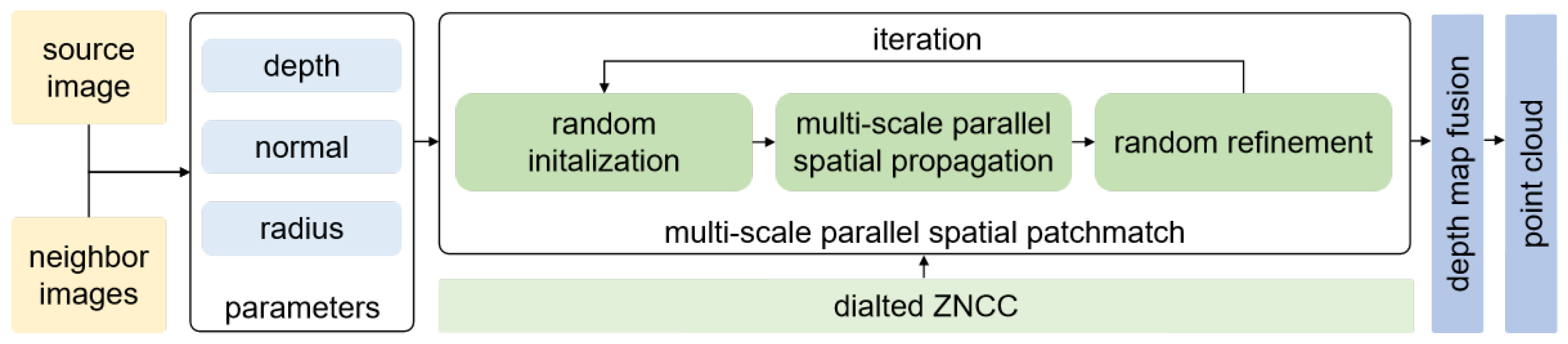
In this paper, we propose MVP-Stereo, a novel multi-view patchmatch stereo method. On the one hand, we introduce a multi-view dilated zero-mean normalized cross-correlation (ZNCC) to deal with low texture and repeated texture with a dilated matching window to avoid increasing computation complexity, inspired by dilated convolution [65]. On the other hand, we propose a multi-scale parallel patchmatch implemented by compute unified device architecture (CUDA), which contains random initialization, multi-scale parallel spatial propagation, random refinement, and the coarse-to-fine strategy. Unlike Gipuma [16], ACMM [37], and ACMMP [38] directly performing parallel spatial propagation, our method proposes multi-scale parallel spatial propagation, which splits pixels into pixel blocks with different scales and propagates the best plane parameters in each pixel block to accelerate converge speed. To validate the proposed method, we conduct qualitative and quantitative experiments on the Strecha dataset [66] and the ETH3D benchmark [67], and compare with state-of-the-art methods like COLMAP [47], OpenMVS [15,44], Gipuma [16], ACMM [37], ACMMP [38], and SD-MVS [53]. We further build a UAV dataset containing three scenes to evaluate the performance of MVS-Stereo. Experimented results show that our method, MVP-Stereo, can achieve competitive reconstruction quality with the highest efficiency. Our contributions are as follows:

1. We introduce a multi-view dilated ZNCC, which can dynamically adjust the matching window size by calculating image variance and reducing computational complexity through a dilated window strategy.

2. We propose a multi-scale parallel patchmatch method, which runs on the GPU, with the multi-scale parallel spatial propagation and the coarse-to-fine strategy to speed up the convergence of depth maps.

3. We propose MVP-Stereo, a multi-view patchmatch stereo method, which achieves competitive reconstruction quality with the highest reconstruction efficiency compared to state-of-the-art methods.

This paper is organized as follows: Section 2 presents details of the proposed method, whereas Section 2.1 describes preliminary knowledge of patchmatch stereo and Section 2.2 introduces our method MVP-Stereo. In Section 3, we conduct qualitative and quantitative experiments on three datasets and compare our method with state-of-the-art methods. The paper is finally concluded in Section 4.

2. Methods

In this section, we provide details of the proposed method. We briefly introduce the patchmatch stereo in Section 2.1 to establish preliminary knowledge. We then present our method MVP-Stereo in Section 2.2, as Figure 1 shows. Specifically, we first describe parameters that need to be estimated, including the depth, the normal, and the window radius. We then introduce how to calculate the multi-view photometric consistency based on the multi-view dilated ZNCC inspired by dilated convolution [65]. We finally explain the multi-scale parallel patchmatch implemented by CUDA.

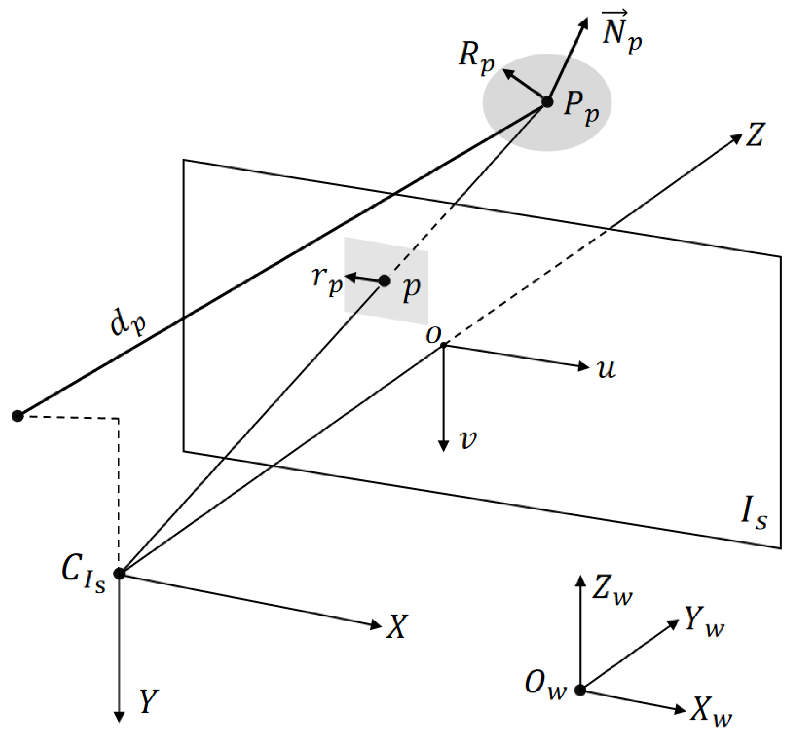
2.1. Patchmatch Stereo

Given two rectified images $I_i$ and $I_j$, patchmatch stereo [43] aims to find a corresponding pixel $p_j$ in image $I_j$ for each pixel $p_i$ in image $I_i$ to maximizes photometric consistency, as Equation (1) shows, where m is the aggregated matching cost, $W_{p_i}$ is the window around $p_i$, $f_{p_i}\left(p\right)$ is the matched pixel defined by the disparity $f_{p_i}$ around the pixel $p_i$, $\mathcal{F}$ is the set of all possible plane hypotheses.

$$\underset{f\in \mathcal{F}}{argmin}\sum _{p_i\in I_i,p\in W_{p_i}}m(I_i\left(p\right),I_j\left(f_{p_i}\left(p\right)\right))$$

(1)

Unlike other stereo estimation methods that rely on the front-parallel assumption [40], patchmatch stereo defines a slanted plane for each pixel $p_i$ using three parameters $a_{f_{p_i}},b_{f_{p_i}},c_{f_{p_i}}$ to calculate the matched pixel $p_j$, as shown in Equation (2), where $x_{p_i},y_{p_i}$ is the position of $p_i$ on the image plane.

$$p_j=f_{p_i}\left(p\right)=p-(a_{f_{p_i}}{x}_{p_i}+b_{f_{p_i}}{y}_{p_i}+c_{f_{p_i}})$$

(2)

As the size of $\mathcal{F}$ is infinite, it is impossible to directly build a cost volume to find the best plane. Patchmatch stereo solves this problem using an iterative randomized method containing random initialization, spatial propagation, and random refinement.

The random initialization assigns an initial plane to each pixel. Although it is impossible to correctly set the plane parameters for all pixels through random initialization, some pixels can be assigned the correct plane parameters by chance. For example, if we assume the probability of a pixel being assigned the correct plane parameters randomly is c, the probability that all pixels in an image of width w and height h are assigned incorrect planes is ${(1-c)}^{wh}$, which approaches zero for high-resolution images.

After random initialization, patchmatch stereo uses spatial propagation and random refinement to find the optimal plane parameters for each pixel in $I_i$ through several iterations. Spatial propagation aims to identify better plane parameters from nearby pixels, and random refinement aims to find better plane parameters through random searching from all possible plane parameters. During each iteration, patchmatch stereo starts from the top left or bottom right of the image and sequentially updates the plane parameters for each pixel, as Figure 2 shows. Patchmatch stereo can reconstruct high-quality disparity maps within three iterations, and each pixel only needs four neighboring pixels in the spatial propagation and six random searches in the random refinement.

2.2. MVP-Stereo

Following patchmatch stereo [43], we propose MVP-Stereo, a multi-view patchmatch stereo method to iteratively reconstruct the depth map. Firstly, we explain how to define a slanted plane for each pixel and the corresponding parameters that need to be estimated in Section 2.2.1. Secondly, in Section 2.2.2, we propose the dilated ZNCC to address low-texture or repeated texture and extend the dilated ZNCC to multi-view. Finally, we describe the details of multi-scale parallel patchmatch in Section 2.2, which contains random initialization, multi-scale parallel spatial propagation, random refinement, and the coarse-to-fine strategy. After reconstructing the depth map, MVP-Stereo follows [15,39] to filter out noise, re-project the depth map to 3D space and generate the point cloud.

To simplify the following introduction, we define some symbols. Each source image $I_S$ has several neighbor images $I_{N_i},(1<=i<=m)$, with intrinsic parameters $K_{I_S},K_{I_{N_i}}$ and extrinsic parameters, including rotation $R_{I_S},R_{I_{N_i}}$ and camera center $C_{I_S},C_{I_{N_i}}$.

2.2.1. Estimated Parameter

Similar to patchmatch stereo [43], which builds a slanted plane to estimate the disparity of each pixel, MVP-Stereo also assumes that each pixel p in image $I_S$ is located on a plane $f_p$ [15,16,37,38]. However, instead of using $f_p$ to estimate the disparity, which is only workable for two views, MVP-Stereo directly estimates the parameter of a 3D plane $f_p$. Generally, $f_p$ has three types of parameters, including the central point of the plane $P_p=(X_{P_p},Y_{P_p},Z_{P_p})$, the plane normal ${\overrightarrow{N}}_p=(X_{\overrightarrow{N}p},Y_{\overrightarrow{N}p},Z_{\overrightarrow{N}p})$, and the plane radius $R_p$, as shown in Figure 3.

According to the multi-view geometry (MVG) [45], $P_p$ can be re-parameterized by the depth $d_p$ through $P_p=d_p{K}_{I_S}^{-1}\tilde{p}$ to reduce freedom from three to one, where $\tilde{p}$ is the homograph representation of p. Meanwhile, we re-parameter the plane radius $R_p$ by the window radius around the pixel p on the image plane to simplify the calculation, based on the assumption that nearby pixels are on the same plane. Therefore, MVP-Stereo needs to estimate the depth $d_p$, the normal ${\overrightarrow{N}}_p$, and the window radius $r_p$.

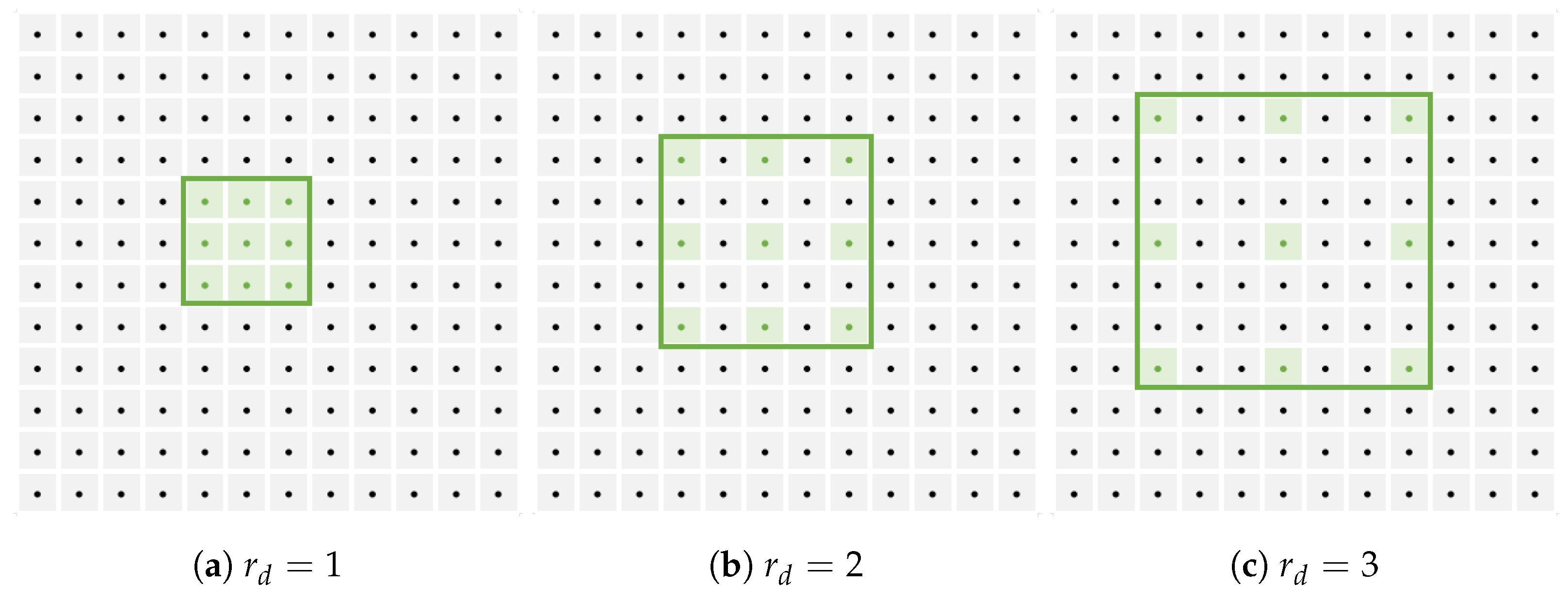
2.2.2. Multi-View Dilated ZNCC

Given a plane $f_p$, we use the ZNCC, which is suitable for high-resolution images [15], to calculate photometric consistency to determine the best plane parameter, as Equation (3) shows, where $f_p(p,I_{N_i})$ is the matched pixel on one of the neighbor images $I_{N_i}$, $W_p$ is the set of pixels within a window of radius $r_p$ around p, ${\overline{I}}_r\left(p\right)$ is the average pixel value within the window around p, and ${\overline{I}}_{N_i}\left(f_p\left(p\right)\right)$ is the average pixel value within the window around $f_p\left(p\right)$. In practice, we use $ZNCC=1-ZNCC$ to denote photometric consistency, with smaller values indicating higher similarity.

$$ZNCC(I_S,I_{N_i},p,f_p)=\frac{{\sum }_{j\in W_p}(I_S\left(j\right)-{\overline{I}}_S\left(p\right))(I_{N_i}\left(f_p(j,I_{N_i})\right)-{\overline{I}}_{N_i}\left(f_p(p,I_{N_i})\right))}{\sqrt{{\sum }_{j\in W_p}{(I_S\left(j\right)-{\overline{I}}_S\left(p\right))}^2{\sum }_{j\in W_p}{(I_{N_i}\left(f_p(j,I_{N_i})\right)-{\overline{I}}_{N_i}\left(f_p(p,I_{N_i})\right))}^2}}$$

(3)

Based on the MVG [45], $f_p$ estimates the matched pixel of p on $I_{N_i}$ through homograph mapping $f_p(p,I_{N_i})=H_{S{N}_i}\tilde{p}$, where $H_{S{N}_i}$ is defined in Equation (4).

$$H_{S{N}_i}=K_{N_i}(R_{N_i}{R}_S^{-1}+\frac{R_{N_i}(C_S-C_{N_i}){\overrightarrow{N}}_p^T}{{\overrightarrow{N}}_p^T[p;d_p]})K_S^{-1}$$

(4)

However, ZNCC only works for two views, and we can not directly average photometric consistency to extend ZNCC to multi-views, since a pixel p on the source image $I_S$ may not be visible to all neighbor images because of occlusions. Therefore, we define a minimal photometric consistency threshold $Z_{min}$ to filter out the neighbor image whose ZNCC is beyond the threshold and mark this image as invisible for this pixel. In the end, we only average the ZNCC on visible images, as shown in Equation (5), where $I_V$ is the set of visible images and belongs to $I_N$, $|I_V|$ is the size of the visible images. As for the plane with no visible images, we directly set the multi-view matching cost to $Z_{max}$.

$$ZNCC(I_S,p,f_p)=\left\{\begin{array}{cc}\frac{{\sum }_{v\in I_V}ZNCC(I_S,I_v,p,f_p)}{|I_V|};\hfill & |I_V|>=1\hfill \\ Z_{max};\hfill & |I_V|=0\hfill \end{array}\right.$$

(5)

Although ZNCC achieves impressive reconstruction quality, it still suffers from low texture and repeated texture problems. Xu and Tao [37], Xu et al. [38], Romanoni and Matteucci [49] try to overcome this limitation by introducing external constraints, and Xu et al. [50] improves the reconstruction quality by increasing the window radius $r_p$, but all of these methods increase the computational complexity. Inspired by the dilated convolution [65], we propose dilated ZNCC to balance the accuracy and the efficiency, which utilizes a portion of pixels within the window to calculate photometric consistency, as Figure 4 shows. For low texture and repeated texture areas, we increase $r_p$ to improve the reception field of ZNCC without increasing the computational complexity. However, unquestioningly increasing $r_p$ will lead to over-smooth reconstruction results. Therefore, we propose a dynamic window adjustment strategy that strives to find a balance between $r_d$ and the reconstruction quality, as Equation (6) shows, where ${\sigma }_p$ is the variance of the pixel values within the window around p, and $\beta =exp(-max({\sigma }_p/T_{\sigma }-1,0))$. The pixel p with ${\sigma }_p$ lower than $T_{\sigma }=0.005$ is considered as low texture or repeated texture.

$$ZNCC(I_S,p,f_p)=(\frac{\beta }{r_p}+(1-\beta )r_p)ZNCC(I_S,p,f_p)$$

(6)

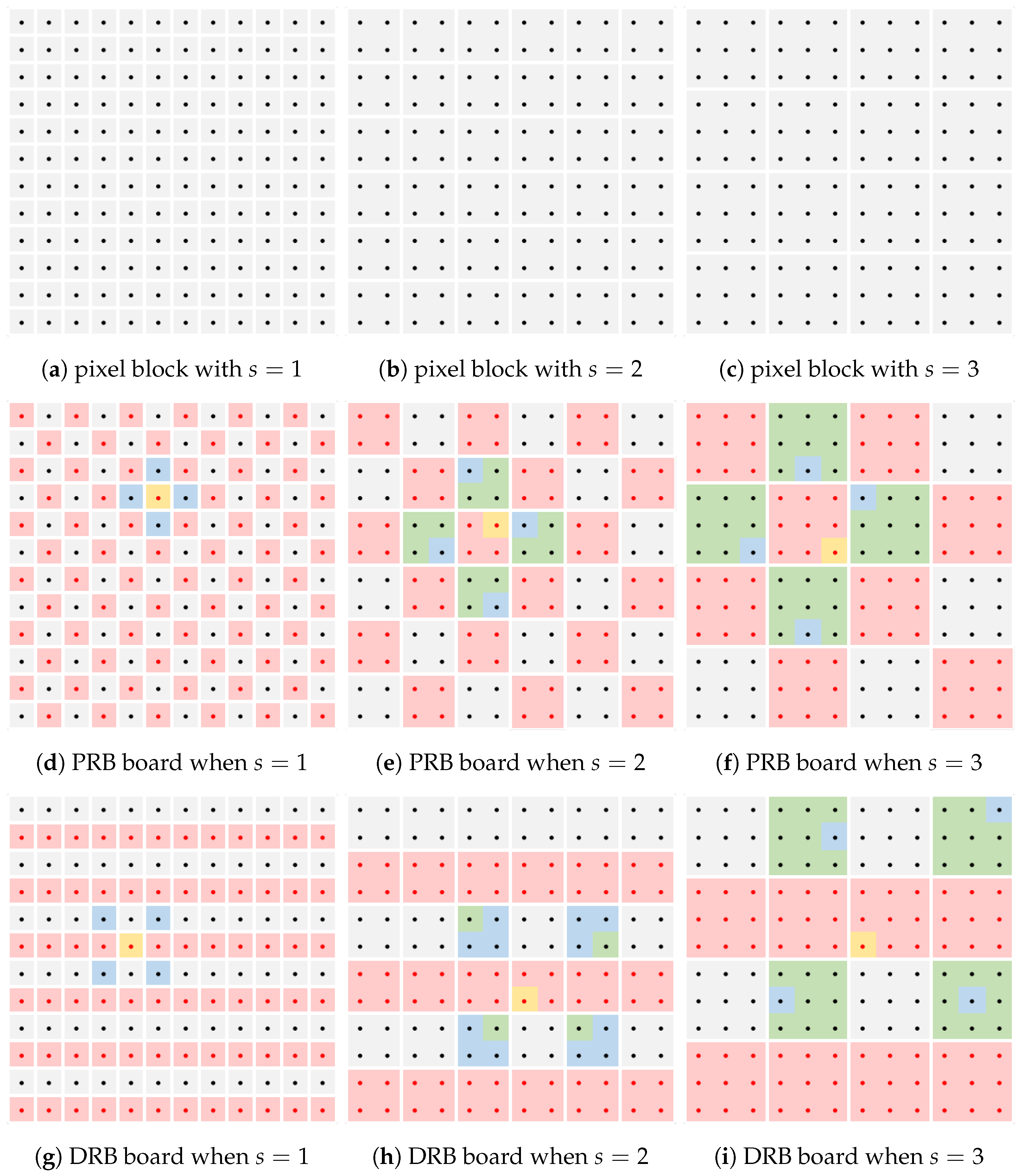
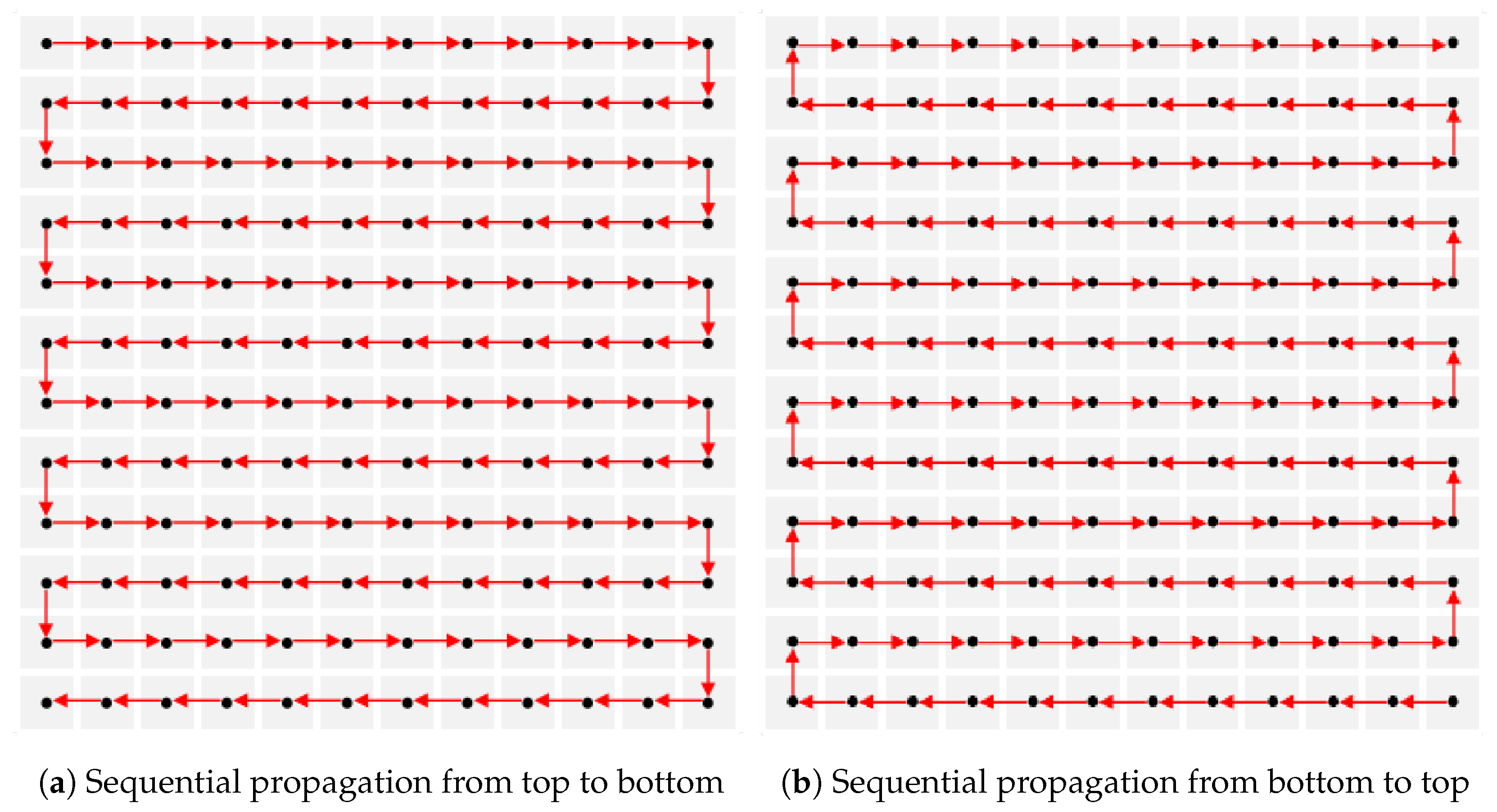
2.2.3. Multi-Scale Parallel Patchmatch

Our method MVP-Stereo reconstructs the dense point cloud based on the depth map fusion [24,26], and its core module is multi-scale parallel patchmatch (MSP-Patchmatch) using multi-view dilated ZNCC, which reconstructs the depth map of the source image $I_S$ through random initialization, multi-scale parallel spatial propagation, random refinement, and the coarse-to-fine strategy. In this section, we describe the details of MSP-Patchmatch.

Random initialization: According to Section 2.2.1, we need to initialize three types of parameters for all pixels in the source image $I_S$, including the depth, the normal, and the window radius. The initial depth $d_{init}$ is randomly selected between the minimum depth $d_{min}$ and the maximum depth $d_{max}$, as Equation (7) shows, where ${\delta }_d$ is a random number between 0 and 1 following the normal distribution. The initial normal ${\overrightarrow{N}}_{init}$ is randomly generated by Equation (8) following Gipuma [16], where ${\delta }_{n_1}$ and ${\delta }_{n_2}$ are two random number between 0 and 1 following the normal distribution. As for the initial window radius, we set $s_{init}=1$.

$$d_{init}=d_{min}+(d_{max}-d_{min}){\delta }_d$$

(7)

$${\overrightarrow{N}}_{init}=(1-2S,2{\delta }_{n_1}\sqrt{1-S},2{\delta }_{n_2}\sqrt{1-S}),S=({\delta }_{n_1}^2+{\delta }_{n_2}^2)<1$$

(8)

Multi-scale parallel spatial propagation: Unlike patchmatch stereo, which performs sequentially spatial propagation, MSP-Patchmatch utilizes multi-scale parallel spatial propagation. The straightforward way to apply parallel spatial propagation is utilizing the red–black board [16], which only updates half of the pixels in each iteration. However, parallel spatial propagation is easy to stack in local minimal and needs more plane hypotheses from adjacent pixels [16,37,38]. To deal with this problem, we propose a multi-scale parallel spatial propagation pipeline. First, We build a multi-scale red–black board by dividing all pixels into several blocks of different sizes. We then build the perpendicular red–black board (PRB board) and the diagonal red–black board (DRB board), where each red block in the PRB board has four adjacent black boards from top, down, left, and right. At the same time, each red block in the DRB board has four adjacent black boards from left–up, right–up, right–down, and left–down. Compared to using a PRB board alone, a DRB board improves the propagation speed. When diagonally adjacent blocks have better planar parameters, a DRB board requires one propagation, while a PRB board requires two propagations. Finally, we parallelly propagate plane parameters between adjacent blocks. More specifically, we first find out the best plane parameters by the multi-view dilated ZNCC in each block, then propagate adjacent plane parameters to the central block, and finally find the best plane parameters. Therefore, MSP-Patchmatch finds the best plane parameters in a pixel block and only updates a portion of pixels. Figure 5 shows how to build a multi-scale red–black board on a $12\times 12$ image with block size ranges from 1 to 3 and how to propagate plane parameters. In MVP-Stereo, we build a multi-scale red–black board with block size ranges from $s_{min}=1$ to $s_{max}=6$. We conduct $P_{iter}$ iterations and perform spatial propagation from a larger block size to a smaller one in each iteration.

Random refinement: In each iteration, we refine the plane parameters with random refinement after spatial propagation. Random refinement contains local and global random searching. Local random searching perturbs the current plane parameters within a neighborhood and selects the best plane parameters that maximize multi-view photo consistency. Equation (9) shows how to generate the random depth $d_{sear}$, where ${\xi }_d$ is the searching scale and ${\delta }_d$ is a random number. Equation (10) generates the random normal ${\overrightarrow{N}}_{sear}$, where ${\xi }_n$ is the searching scale and ${\overrightarrow{N}}_{init}$ is coming from Equation (8). As for the window radius, we generate a random scale in each search as Equation (11) shows, where $r_{min}=1$ and $r_{max}=6$ are the minimal and maximum window radius. Meanwhile, the global random searching only applies when the propagation fails to find valid plane parameters, i.e., $ZNCC(I_S,p,f_p)>Z_{max}$. During the global random searching, the random depth comes from Equation (7), the random normal comes from Equation (8), and the random window radius comes from Equation (11). We conduct $R_{iter}$ random searching during each iteration behind spatial propagation.

$$d_{sear}=d_{old}+(d_{max}-d_{min}){\xi }_d{\delta }_d$$

(9)

$${\overrightarrow{N}}_{sear}={\overrightarrow{N}}_{old}+{\overrightarrow{N}}_{init}{\xi }_n,\left|\right|{\overrightarrow{N}}_{sear}{\left|\right|}_2=1$$

(10)

$$s_{init}=(r_{max}-r_{min})*{\delta }_r+r_{min}$$

(11)

Coarse-to-fine: In addition, we use the coarse-to-fine strategy as ACMM [37] and ACMMP [38] do, where we reconstruct the coarse depth map at low-resolution images and then estimate the fine depth map at original resolution images. However, we do not use random initialization at the fine stage. We initialize the fine stage by upsampling the depth map and normal map directly from the coarse stage and setting $r_p=1$. In addition, we reduce searching scales ${\xi }_d$ and ${\xi }_n$ in the fine stage in anticipation of obtaining finer planar parameters. Specifically, we set ${\xi }_d=0.1,{\xi }_n=0.1$ at the coarse stage and ${\xi }_d=0.01,{\xi }_n=0.01$ at the fine stage.

3. Experiments

3.1. Datasets

We conduct qualitative and quantitative experiments on two datasets, including the Strecha dataset [66] and the ETH3D benchmark [67]. The Strecha dataset contains two scenes with ground truth depth maps, including Fountain and Herzjuse. The ETH3D benchmark comprises several indoor and outdoor scenes and is divided into training and test splits. The training split contains 13 scenes for tuning our method and verifying the effectiveness of each component. The test split contains 12 scenes for evaluating different approaches. In addition, we further qualitatively evaluate our method on three datasets captured by a UAV.

Table 1. Details of three datasets. Superscripts 1, 2, 3, and 4 indicate indoor scenes in the train split, outdoor scenes in the train split, indoor scenes in the test split, and outdoor scenes in the test split in the ETH3D benchmark, respectively.

Datasets	Scene	Image Number	Resolution
Strecha [66]	Fountain, Herzjesu	11, 8	$3072\times 2048$
ETH3D [67]	(courtyard, electro, facade, meadow, playground, terrace) 1, (delivery_area, kicker, office, pipes, relief, relief_2, terrains) 2, (boulders, observatory, terrace_2) 3, (botanical_garden, bridge, door, exhibition_hall, lecture_room, living_room, lounge, old_computer, statue) 4	(38, 45, 76, 15, 38, 23) 1, (44, 31, 26, 14, 31, 31, 42) 2, (26, 27, 13) 3, (30, 110, 7, 68, 23, 65, 10, 54, 11) 4	around $6200\times 4130$
UAV	P104	104	$5472\times 3468$
	P114	114	$5456\times 3632$
	P139	139	$6000\times 4000$

represents details of used datasets in our experiments.

3.2. Implementation

We implement our method MVP-Stereo on CUDA in Visual Studio 2015. To be as efficient as possible, we use the texture memory to store the reference image and the neighbor images. Meanwhile, we utilize curandGenerateUniform to generate random numbers efficiently. In all experiments, we use a personal computer (PC) equipped with an NVIDIA RTX1080Ti, 64G RAM (random access memory), and an Intel i5 processor. Moreover, we use uniform hyperparameter settings on all datasets. We set $W_p=5$, $Z_{min}=0.3$, $Z_{max}=0.6$ in the multi-view dialted ZNCC. We set $P_{iter}=6,R_{iter}=6$ in the multi-scale parallel spatial patchmatch. As for $d_{min}$ and $d_{max}$, we obtain them from the sparse points provided by COLMAP [9].

3.3. Evaluation Metrics

We follow ACMM [37] and ACMMP [38] to evaluate the reconstruction quality of different methods. On the Strecha dataset, we evaluate the quality of depth maps reconstructed by different methods. For each reconstructed depth map, the quality is calculated by the percent of pixels whose distance between the ground truth depth map is below the threshold $T_d$. On the ETH3D benchmark, we evaluate point clouds generated by different methods, including completeness, accuracy, and F1. The completeness is calculated by counting the percent of points in the ground truth point cloud whose distance from the nearest point in the reconstructed point cloud is below the threshold $T_c$. The accuracy is calculated by counting the percent of points in the reconstructed point cloud whose distance from the nearest point in the ground truth point cloud is below the threshold $T_c$. As the completeness and the accuracy are complementary, we also calculate F1, which averages the completeness and the accuracy. In addition to the reconstruction quality, we measure the time required to reconstruct the point cloud to evaluate the reconstruction efficiency of different methods. Generally, quality, completeness, accuracy, and F1 are measured in percentages without units, while efficiency is measured in seconds. We compare our method with several state-of-the-art methods, including COLMAP [47], OpenMVS [15,44], Gipuma [16], ACMM [37], ACMMP [38], and SD-MVS [53]. In all experiments, we set $T_d$ = 2 cm, 10 cm and $T_c$ = 2 cm, 10 cm.

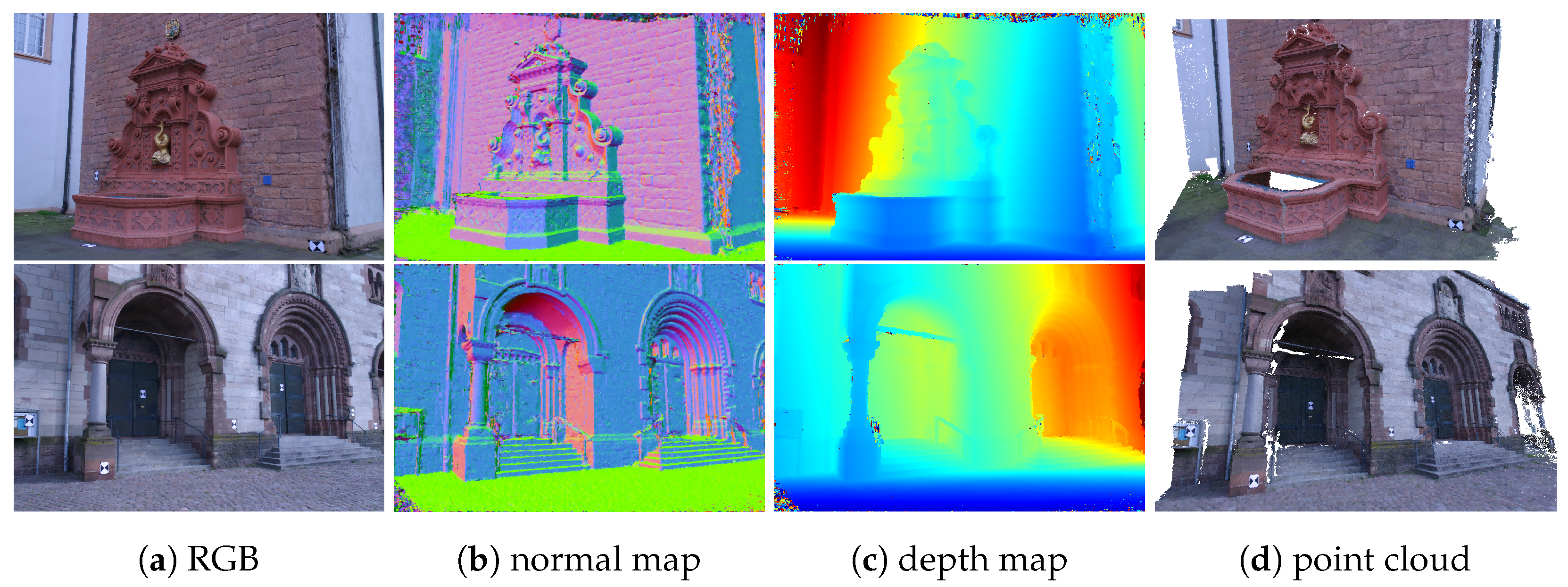
3.4. Experiments on the Strecha Dataset

Table 2. Reconstruction quality and reconstruction time on the Strecha dataset [66]. ↑ means the higher the better, and ↓ means the lower the better.

Method	Fountain			Herzjesu
		Quality (%)			Quality (%)
	Time (s)↓	Td = 2 cm↑	Td = 10 cm↑	Time (s)↓	Td = 2 cm↑	Td = 10 cm↑
COLMAP [47]	1046.88	82.7	97.5	709.14	69.1	93.1
OpenMVS [15,44]	191.13	77.1	90.7	150.48	65.5	82.2
Gipuma [16]	235.58	69.3	83.8	134.34	28.3	45.5
ACMM [37]	321.66	85.3	97.4	141.26	73.1	93.2
ACMMP [38]	395.48	84.8	97.2	248.28	72.6	93.5
Ours	81.21	80.6	93.1	54.10	65.6	84.6

shows the quantitative results on the Strecha dataset. When $T_{depth}$ = 2 cm, our method achieves $97.5\%$, $94.5\%$, and $95.1\%$ of the reconstruction quality of COLMAP [47], ACMM [37], and ACMMP [38] on the Fountain scene, while only requiring $7.8\%$, $25.3\%$, and $20.5\%$ of their reconstruction time, respectively. On the Herzjesu scene, our method achieves $94.9\%$, $89.7\%$, and $91.5\%$ of the reconstruction quality of COLMAP, ACMM, and ACMMP using only $7.6\%$, $38.3\%$, and $21.8\%$ of their reconstruction times, respectively. When $T_{depth}=10$ cm, the difference in reconstruction quality between our method and COLMAP, ACMM, and ACMMP remains small. Meanwhile, on both Fountain and Herzjesu scenes, our method outperforms OpenMVS [15,44] and Gipuma [16] in reconstruction quality and reconstruction time, using approximately one-third of their time but obtain higher quality. Overall, our method demonstrates the highest reconstruction efficiency among all methods while achieving competitive reconstruction quality compared to state-of-the-art methods.

The reconstruction results of our method are shown in Figure 6, including normal maps, depth maps, and point clouds. Different colors in the normal map mean different orientations. Different colors in the depth map indicate different distances, where blue is closer and red is farther. Different colors of the point cloud are obtained by projecting each point onto the image plane and sampling the RGB information. These visualization results show that our method can reconstruct high-quality point clouds with a simple random search and parallel propagation.

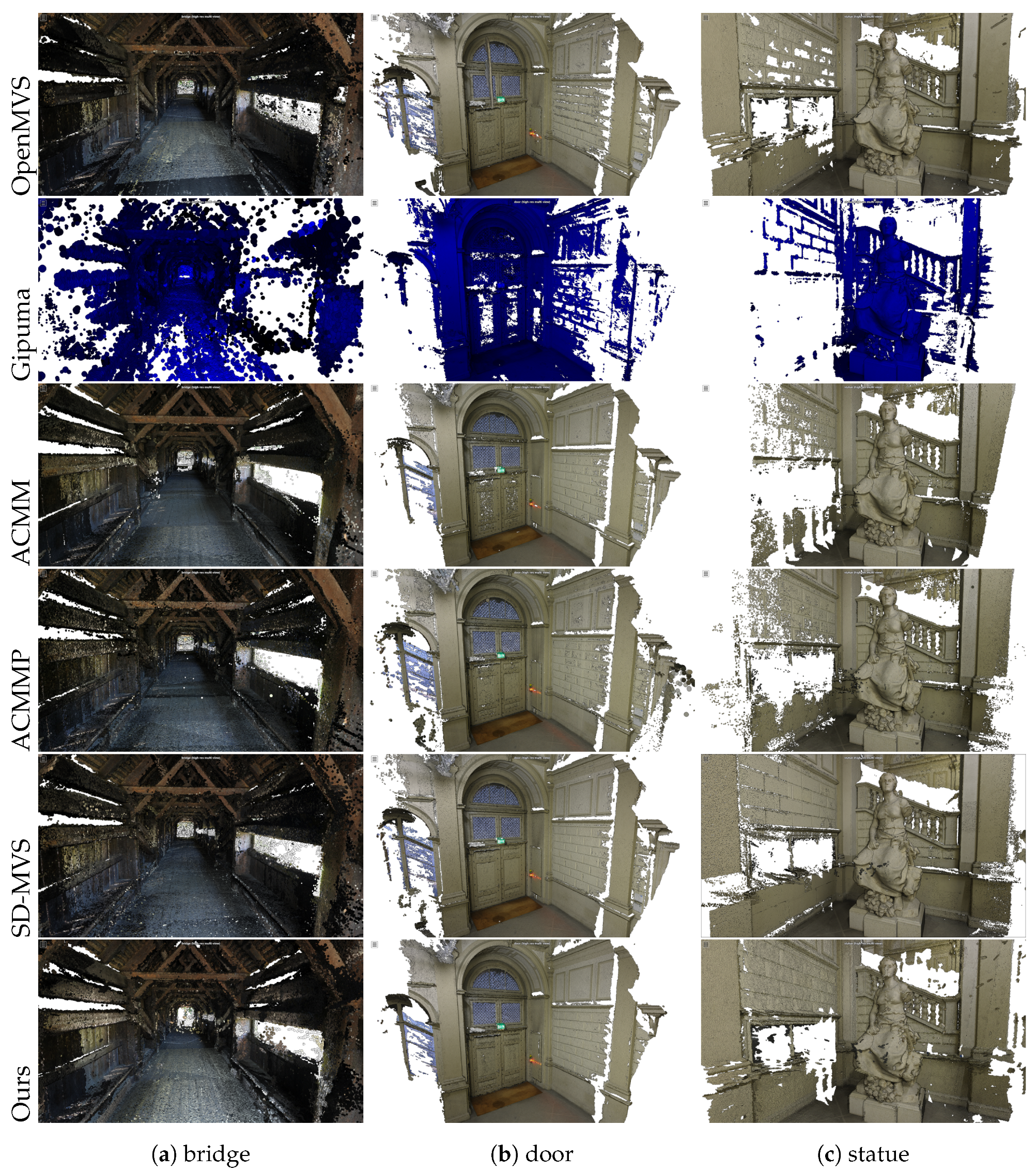
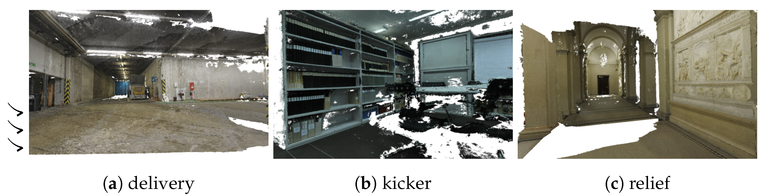
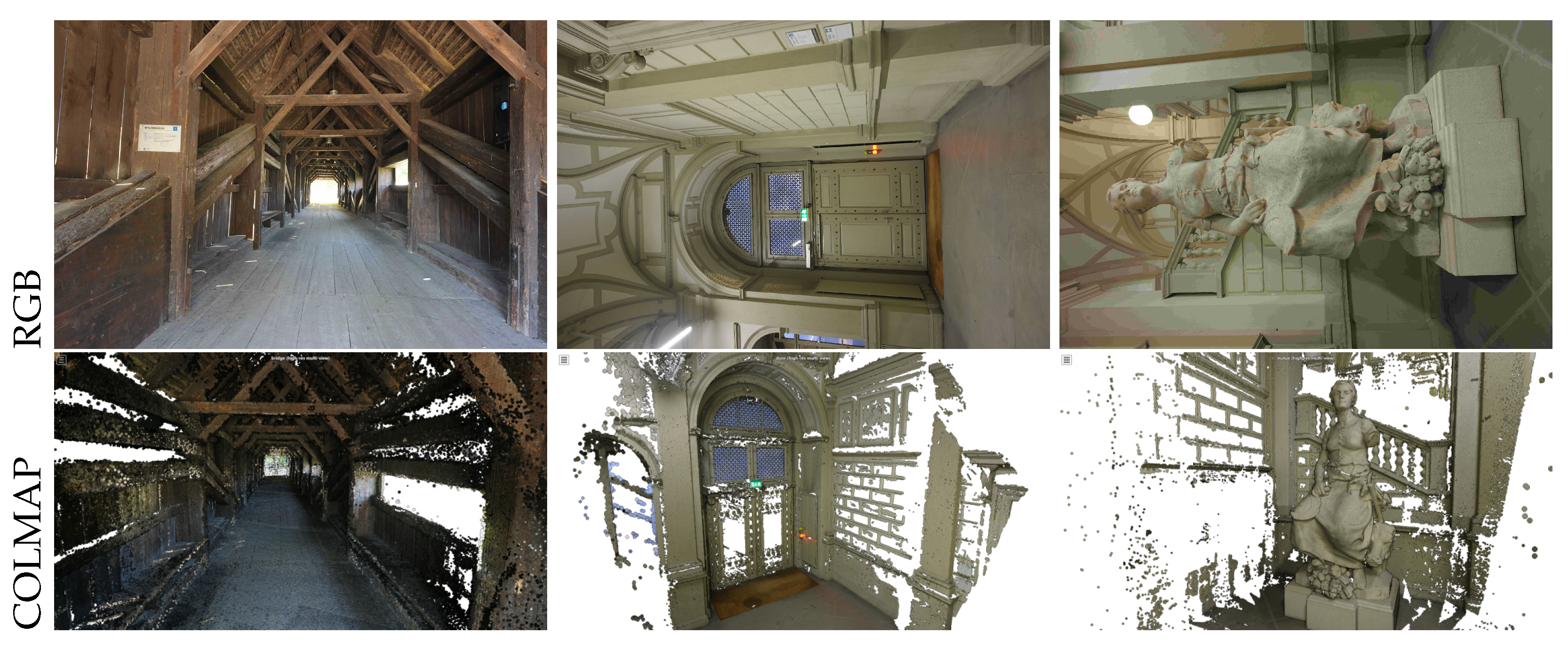
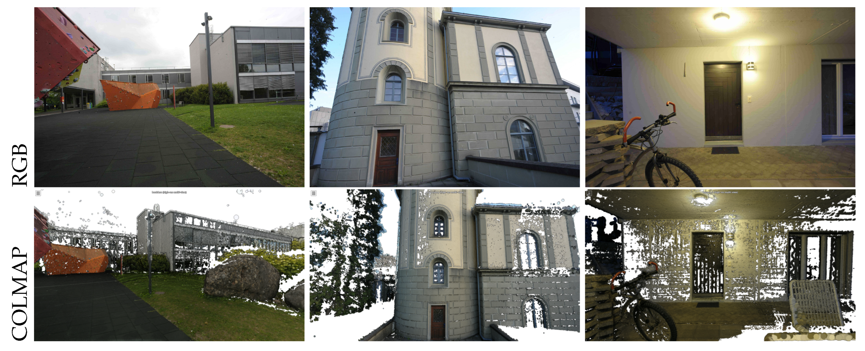
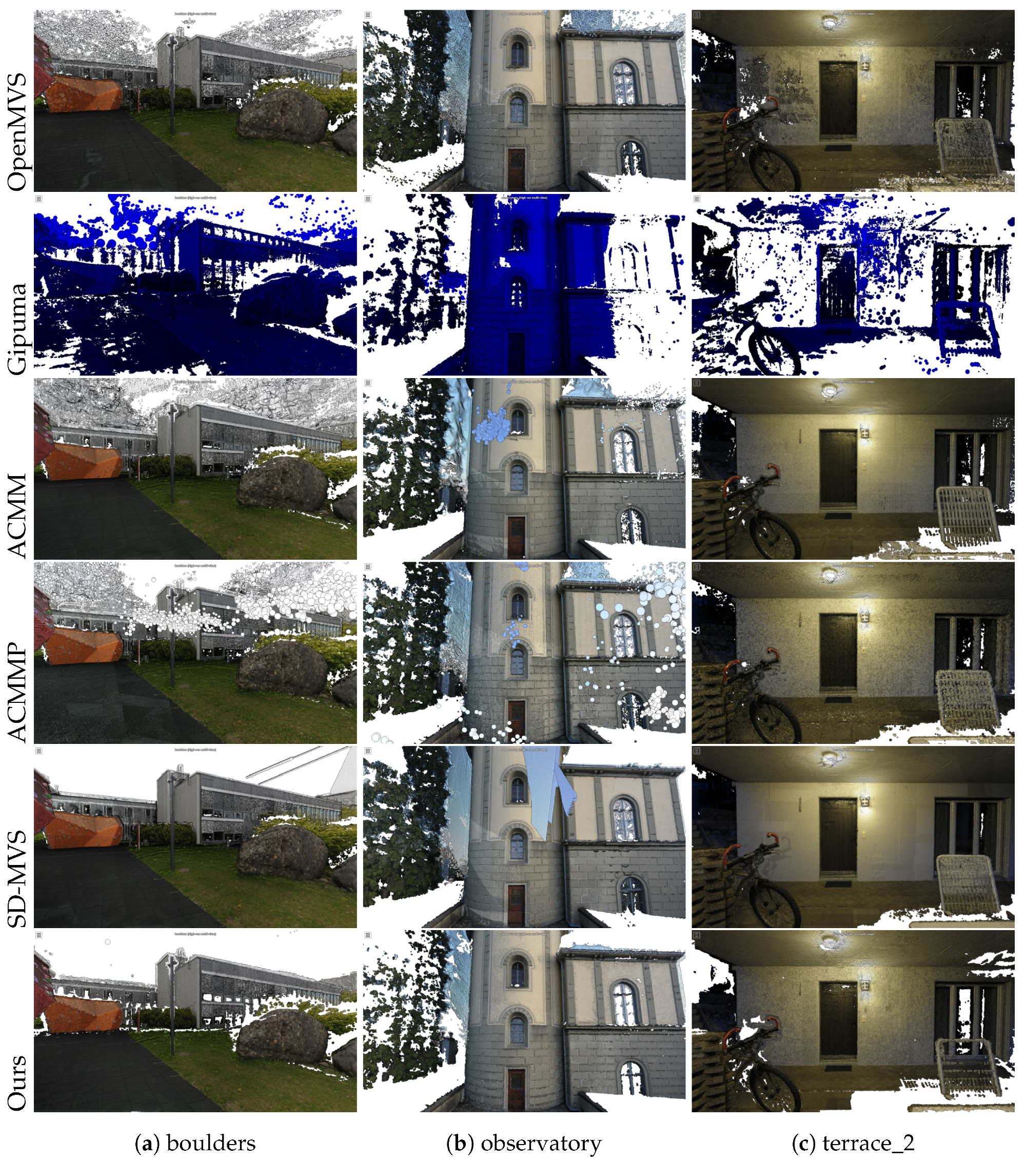
3.5. Experiments on the ETH3D Benchmark

We quantitatively evaluate our method on the test split of the ETH3D benchmark and show results in

Table 3. Reconstruction quality and reconstruction time on the test split of the ETH3D benchmark. ↑ means the higher the better, and ↓ means the lower the better.

	Method		${\mathit{T}}_{\mathit{c}}$ = 2 cm (%)			${\mathit{T}}_{\mathit{c}}$ = 10 cm (%)
		Time (s)↓	comp↑	acc↑	F1↑	comp↑	acc↑	F1↑
indoor	COLMAP [47]	1869.33	59.65	91.95	70.41	82.82	98.11	89.28
	OpenMVS [15,44]	2263.08	75.92	82.00	78.33	88.84	95.20	91.68
	Gipuma [16]	767.00	31.44	86.33	41.86	52.22	98.31	65.41
	ACMM [37]	1332.72	72.73	90.99	79.84	88.22	97.79	92.50
	ACMMP [38]	3284.78	86.90	91.36	88.86	97.34	97.76	97.53
	SD-MVS [53]	3055.56	87.49	89.88	88.50	97.40	97.70	97.53
	Ours	533.67	76.23	73.51	74.46	85.83	95.28	90.08
outdoor	COLMAP [47]	1025.33	72.98	92.04	80.81	89.70	98.64	93.79
	OpenMVS [15,44]	1459.67	86.41	81.93	84.09	96.48	96.32	96.40
	Gipuma [16]	458.00	45.30	78.78	55.16	62.40	97.36	75.18
	ACMM [37]	662.07	79.17	89.63	83.58	90.43	98.85	94.35
	ACMMP [38]	1711.67	86.58	90.55	88.32	97.01	98.79	97.87
	SD-MVS [53]	1451.45	86.71	86.22	87.50	97.06	96.35	97.53
	Ours	293.33	79.79	82.71	81.13	88.93	96.92	92.71

. ACMMP [38] achieves the highest F1 score, surpassing other methods. When $T_c$ is set to 2 cm, the F1 of our method reaches $83.80\%$ and $91.86\%$ of ACMMP on indoor and outdoor scenes, respectively. However, our method only requires $16.25\%$ and $17.14\%$ reconstruction time of ACMMP in both the indoor and outdoor datasets. Although SD-MVS [53] ranks second on the F1 score, our method obtains $84.14\%$ and $98.72\%$ of this method with $17.47\%$ and $20.21\%$ reconstruction time on indoor and outdoor scenes. Gipuma [16] is the second most efficient of all the methods, and our method needs $69.58\%$ and $64.05\%$ of its reconstruction time on indoor and outdoor scenes, respectively, but achieves an improvement of $77.88\%$ and $47.07\%$ in F1. While COLMAP [47] achieves the best results in accuracy, it is not good in completeness and reconstruction efficiency. Our method achieves competitive reconstruction quality to OpenMVS [15,44] and ACMM [37], with little difference in F1, but our method only requires roughly one-third of the reconstruction time. Overall, our method achieves the highest reconstruction efficiency on the ETH3D benchmark while guaranteeing a reconstruction quality competitive to state-of-the-art methods. To be noted, all visualization results are available on the ETH3D benchmark through the following link https://www.eth3d.net/result_details?id=1090 (accessed on 1 February 2024).

To further compare different methods, we select three scenes from indoor and outdoor in the test split of the ETH3D benchmark and visualize reconstruction results in Figure 7 and Figure 8. In the indoor scenes, COLMAP [47], OpenMVS [15,44], and Gipuma [16] all suffer from low texture and repeated texture, and there are a large number of empty space in the reconstructed point clouds, especially in the door scene, where the walls do not reconstruct at all. ACMM [37], ACMMP [38], SD-MVS [53], and our methods all recover relatively complete reconstruction results in the indoor scene. In the outdoor scene, the reconstruction quality of all methods is relatively complete, except for Gipuma, which has relatively poor reconstruction quality because the texture is much richer in the outdoor scene. However, ACMM, ACMMP, and SD-MVS, in order to improve the reconstruction quality of the low texture region, are disturbed by the sky region, and there is a lot of noise in the point cloud. Our method effectively removes the influence of the sky by multi-view dialted ZNCC without generating noise.

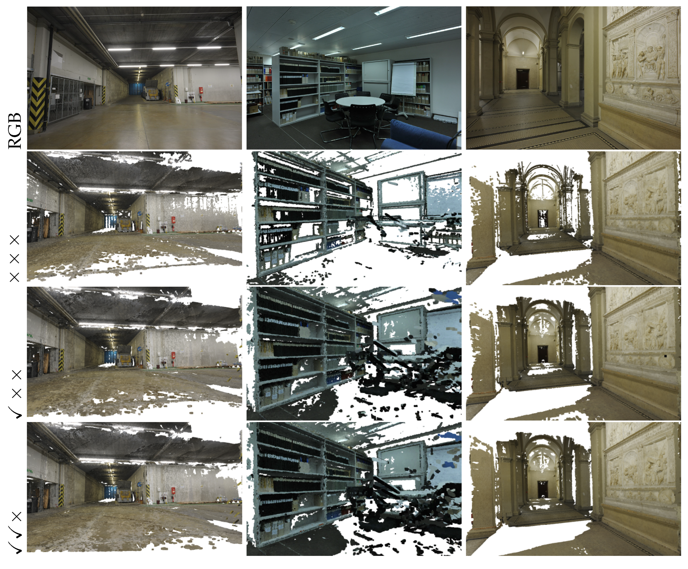
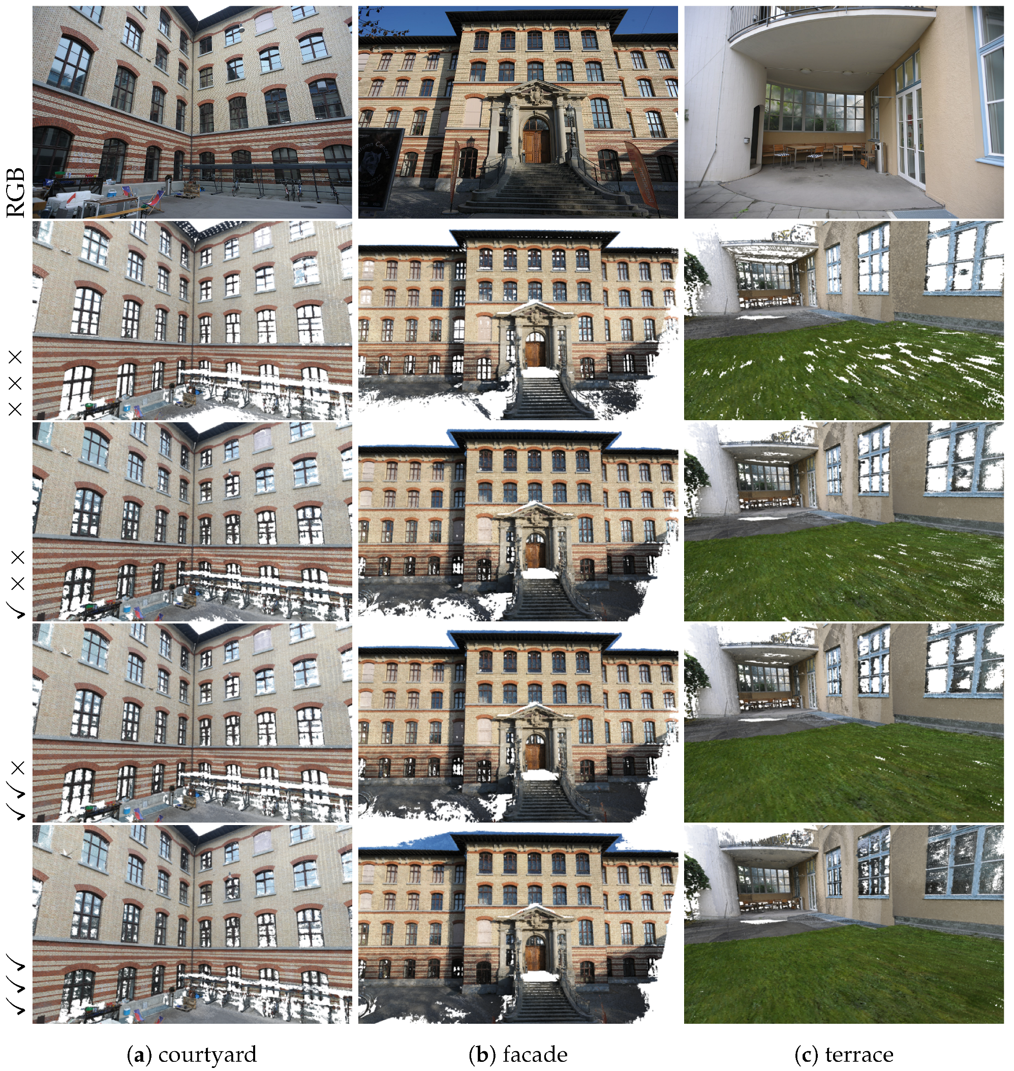
3.6. Ablation Experiments

To verify the effectiveness of proposed modules, including the multi-view dilated ZNCC, multi-scale parallel spatial propagation, and coarse-to-fine, we conduct several ablation experiments on the train split of the ETH3D benchmark. Meanwhile, unlike sequential propagation, which propagates the planar hypothesis among all pixels, multi-scale parallel spatial propagation only propagates the plane hypothesis between nearby pixels. Although increasing the number of iterations $P_{iter}$ can propagate the plane hypothesis further, we analyze how to set $P_{iter}$ to ensure the reconstruction quality.

Table 4. Ablation experiments of different modules in our method. The d-Z indicates the multi-view dilated ZNCC, MSP means multi-scale parallel spatial propagation, and C2F represents the coarse-to-fine strategy. × means not using the module, and ✓ means using the module. ↑ means the higher the better, and ↓ means the lower the better.

				${\mathit{T}}_{\mathit{c}}$ = 2 cm (%)			${\mathit{T}}_{\mathit{c}}$ = 10 cm (%)
	d-Z	MSP	C2F	comp↑	acc↑	F1↑	comp↑	acc↑	F1↑
indoor	×	×	×	50.09	82.21	59.39	67.14	97.51	78.23
	✓	×	×	59.19	77.44	65.26	72.79	95.77	81.69
	✓	✓	×	61.20	78.56	67.07	74.01	95.90	82.51
	✓	✓	✓	70.07	74.39	71.43	82.97	94.70	88.09
outdoor	×	×	×	51.10	76.57	59.70	65.60	97.48	77.30
	✓	×	×	61.35	74.37	66.43	73.57	97.08	83.02
	✓	✓	×	64.13	74.95	68.68	76.23	97.13	84.82
	✓	✓	✓	69.97	72.08	70.60	80.70	95.23	87.32

shows the reconstruction results of different modules in MVP-Stereo on the train split of the ETH3D benchmark. When $T_c$ is set to 2 cm, the F1 score without using any module is 59.39 and 59.70 on indoor and outdoor scenes, respectively. With the help of the multi-view dilated ZNCC, the reconstruction quality of the indoor and outdoor scenes is substantially improved, where the F1 score is 65.26 and 66.43, respectively. The reconstruction quality is further improved after replacing the parallel spatial propagation with multi-scale parallel spatial propagation, where the F1 score is 67.07 and 68.68, respectively. After applying the coarse-to-fine strategy, the F1 score reaches 71.43 and 70.60, respectively. Compared to the version without any proposed modules, MVP-Stereo improves the F1 score by 12.04 and 10.90. MVP-Stereo achieves similar results when $T_c$ is set to 10 cm. Although multi-scale parallel spatial propagation and the coarse-to-fine strategy improve the reconstruction quality, the multi-view dilated ZNCC plays a vital role in improving the reconstruction quality among proposed modules, as the ETH3D benchmark contains lots of low and repeated texture regions.

In order to qualitatively compare the impact of the different modules on the reconstruction quality, we visualize six scenes from the train split of the ETH3D benchmark, as shown in Figure 9 and Figure 10. With the help of different modules, MVP-Stereo successfully deals with low texture and repeated texture areas and reconstructs high-quality point clouds from indoor and outdoor scenes.

Considering that multi-scale parallel spatial propagation propagates between neighboring pixels, MVP-Stereo requires more iterations $P_{iter}$ to improve the reconstruction quality. Therefore, we conduct ablation experiments on $P_{iter}$ to determine how to set it to ensure the reconstruction quality.

Table 5. Ablation experiments on the number of iterations $P_{iter}$. ↑ means the higher the better.

		${\mathit{T}}_{\mathit{c}}$ = 2 cm (%)			${\mathit{T}}_{\mathit{c}}$ = 10 cm (%)
	${\mathit{P}}_{\mathit{iter}}$	comp↑	acc↑	F1↑	comp↑	acc↑	F1↑
indoor	1	27.49	51.49	33.73	45.06	76.63	54.91
	2	66.24	71.99	68.34	80.51	93.23	86.10
	4	68.84	73.73	70.47	82.36	94.39	87.64
	6	70.07	74.39	71.43	82.97	94.70	88.09
outdoor	1	30.80	53.73	37.98	49.18	86.35	61.22
	2	64.93	71.25	67.47	76.00	95.52	84.20
	4	68.77	72.22	69.98	79.62	95.88	86.68
	6	69.97	72.08	70.60	80.70	95.23	87.32

shows reconstruction quality with different iterations on the train split of the ETH3D benchmark. When $T_c$ is set to 2 cm, the F1 score is only 33.73 and 37.98 on indoor and outdoor scenes as $P_{iter}=1$. As $P_{iter}$ gradually increases to 2, 4, 6, there are 34.61, 2.13, and 0.96 improvements in F1 in indoor scenes. At the same time, there are 29.49, 2.51, and 0.62 improvements in F1 scores in outdoor scenes. When $T_c$ = 10 cm, the F1 score is only 54.91 and 61.22 as $P_{iter}=1$. When $P_{iter}$ is gradually raised to 2, 4, 6, the F1 score on indoor scenes has 31.19, 1.54, and 0.45 improvement, while the F1 score has 22.98, 2.48, 0.64 improvement on outdoor scenes. Overall, as $P_{iter}$ increases, the reconstruction quality increases but with more minor improvement. The reconstruction quality is almost not improved much when $P_{iter}=6$, which indicates that MVP-Stereo converges very fast and does not require a lot of iterations. Compared with sequential propagation, which usually requires three iterations to complete convergence, MSP-Patchmatch does not require a high number of iterations.

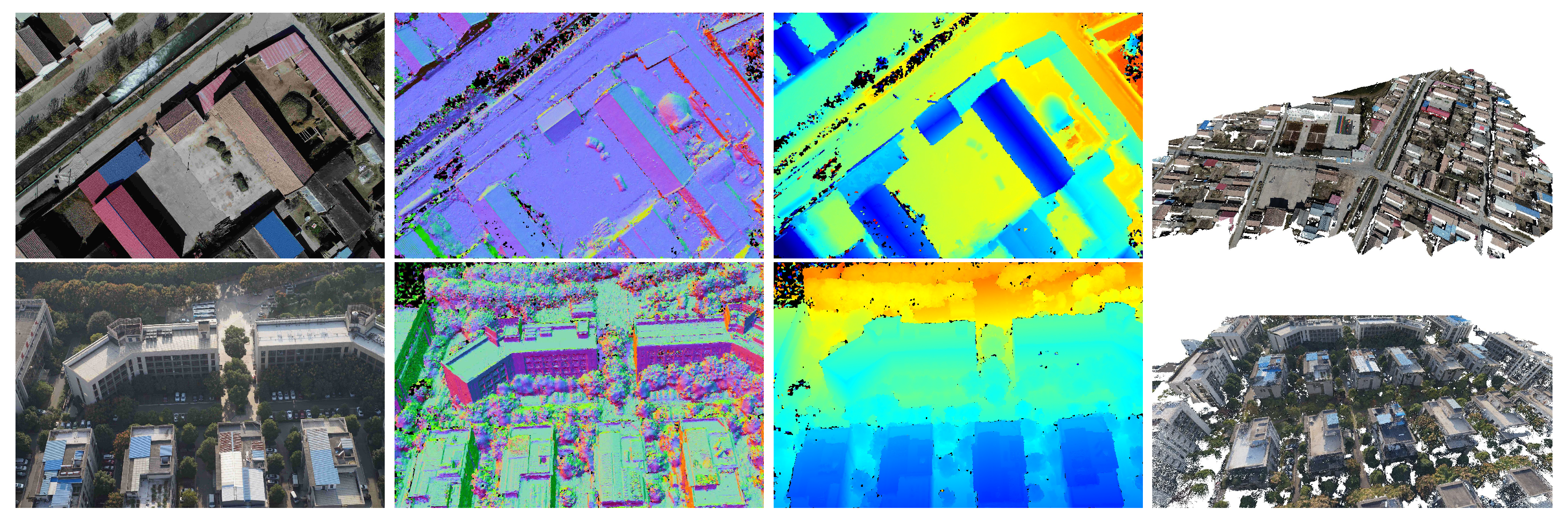
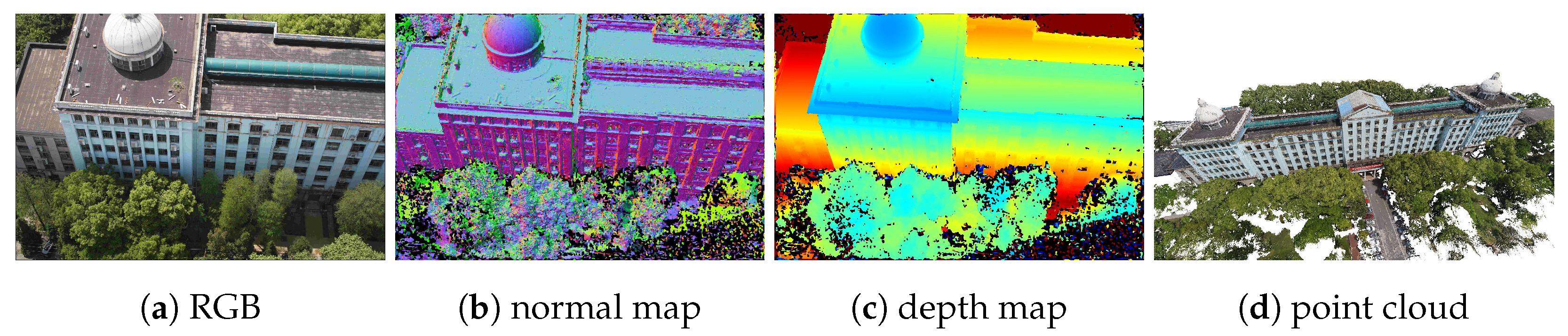
3.7. Experiments on the UAV Dataset

Due to the lack of evaluation datasets in UAV, we use a UAV to collect three scenes to qualitatively evaluate MVP-Stereo. Compared to the Strecha dataset [66] and the ETH3D benchmark [67], the UAV dataset has more images in each scene and covers larger areas with complex structures. As Gipuma [16] and ACMM [37] can not directly handle large scenes, and ACMMP [38] is extremely time-consuming, we compare our method to COLMAP [47] and OpenMVS [15,44].

Table 6. Reconstruction time on the UAV dataset. ↓ means the lower the better.

Method	Time (s) ↓
	P104	P114	P139
COLMAP [47]	5905	6916	8403
OpenMVS [15,44]	4510	6876	7868
Ours	1146	1542	1993

shows the reconstruction time of different methods, where our method is the most efficient and only needs around one-fourth of their time. Without adjusting any parameters, MVP-Stereo can reconstruct high-quality, dense point clouds at P104, P114, and P139, and the reconstruction results are shown in Figure 11.

4. Conclusions

This paper proposes a multi-view parallel patchmatch stereo method, MVP-Stereo, which can reconstruct high-quality point clouds with the highest efficiency. Compared with COLMAP, MVP-Stereo achieves higher reconstruction quality, but only needs one-third of the reconstruction time. Compared with ACMMP and SD-MVS, MVP-Stereo achieves competitive reconstruction quality but only needs one-fifth of the reconstruction time. On the one hand, MVP-Stereo utilizes the multi-view dilated ZNCC to deal with low texture and repeated texture, which dynamically adjusts the window radius based on the image variance and only uses a small portion of pixels to increase the inception field without increasing computation complexity. On the other hand, MVP-Stereo uses MSP-Patchmatch, which uses random initialization, multi-scale parallel spatial propagation, random refinement, and the coarse-to-fine strategy to estimate the depth map and the normal map efficiently. Experiments on the Strecha dataset, the ETH3D benchmark, and the UAV dataset show that our method can achieve competitive results with state-of-the-art methods with the highest reconstruction efficiency. In the future, we plan to improve the reconstruction quality by selecting visible images for each pixel and combining the random refinement with an optimization strategy.

References

1. Zhang, L.; Gruen, A. Multi-image matching for DSM generation from IKONOS imagery. ISPRS J. Photogramm. Remote Sens. 2006, 60, 195–211. [Google Scholar] [CrossRef]
2. Gomez, C.; Setiawan, M.A.; Listyaningrum, N.; Wibowo, S.B.; Hadmoko, D.S.; Suryanto, W.; Darmawan, H.; Bradak, B.; Daikai, R.; Sunardi, S.; et al. LiDAR and UAV SfM-MVS of Merapi volcanic dome and crater rim change from 2012 to 2014. Remote Sens. 2022, 14, 5193. [Google Scholar] [CrossRef]
3. Corradetti, A.; Seers, T.; Mercuri, M.; Calligaris, C.; Busetti, A.; Zini, L. Benchmarking different SfM-MVS photogrammetric and iOS LiDAR acquisition methods for the digital preservation of a short-lived excavation: A case study from an area of sinkhole related subsidence. Remote Sens. 2022, 14, 5187. [Google Scholar] [CrossRef]
4. Nan, L.; Wonka, P. Polyfit: Polygonal surface reconstruction from point clouds. In Proceedings of the IEEE International Conference on Computer Vision, Venice, Italy, 22–29 October 2017; pp. 2353–2361. [Google Scholar]
5. Han, W.; Xiang, S.; Liu, C.; Wang, R.; Feng, C. Spare3d: A dataset for spatial reasoning on three-view line drawings. In Proceedings of the IEEE/CVF Conference on Computer Vision and Pattern Recognition, Seattle, WA, USA, 13–19 June 2020; pp. 14690–14699. [Google Scholar]
6. Hu, Q.; Yang, B.; Xie, L.; Rosa, S.; Guo, Y.; Wang, Z.; Trigoni, N.; Markham, A. Randla-net: Efficient semantic segmentation of large-scale point clouds. In Proceedings of the IEEE/CVF Conference on Computer Vision and Pattern Recognition, Seattle, WA, USA, 13–19 June 2020; pp. 11108–11117. [Google Scholar]
7. Xiang, S.; Yang, A.; Xue, Y.; Yang, Y.; Feng, C. Self-supervised Spatial Reasoning on Multi-View Line Drawings. In Proceedings of the IEEE/CVF Conference on Computer Vision and Pattern Recognition, New Orleans, LA, USA, 18–24 June 2022; pp. 12745–12754. [Google Scholar]
8. Li, Y.; Ge, Z.; Yu, G.; Yang, J.; Wang, Z.; Shi, Y.; Sun, J.; Li, Z. Bevdepth: Acquisition of reliable depth for multi-view 3d object detection. In Proceedings of the AAAI Conference on Artificial Intelligence, Washington, DC, USA, 7–14 February 2023; Volume 37, pp. 1477–1485. [Google Scholar]
9. Schonberger, J.L.; Frahm, J.M. Structure-from-motion revisited. In Proceedings of the IEEE Conference on Computer Vision and Pattern Recognition, Las Vegas, NV, USA, 27–30 June 2016; pp. 4104–4113. [Google Scholar]
10. Moulon, P.; Monasse, P.; Perrot, R.; Marlet, R. Openmvg: Open multiple view geometry. In Proceedings of the Reproducible Research in Pattern Recognition: First International Workshop, RRPR 2016, Cancún, Mexico, 4 December 2016; Revised Selected Papers 1. Springer: Berlin/Heidelberg, Germany, 2017; pp. 60–74. [Google Scholar]
11. Gruen, A. Adaptive least squares correlation: A powerful image matching technique. S. Afr. J. Photogramm. Remote Sens. Cartogr. 1985, 14, 175–187. [Google Scholar]
12. Gruen, A.; Baltsavias, E.P. Geometrically constrained multiphoto matching. Photogramm. Eng. Remote Sens. 1988, 54, 633–641. [Google Scholar]
13. Gruen, A. Least squares matching: A fundamental measurement algorithm. In Close Range Photogrammetry and Machine Vision; Whittler Publishing: Caithness, UK, 1996. [Google Scholar]
14. Agouris, P.; Schenk, T. Automated aerotriangulation using multiple image multipoint matching. Photogramm. Eng. Remote Sens. 1996, 62, 703–710. [Google Scholar]
15. Shen, S. Accurate multiple view 3d reconstruction using patch-based stereo for large-scale scenes. IEEE Trans. Image Process. 2013, 22, 1901–1914. [Google Scholar] [CrossRef]
16. Galliani, S.; Lasinger, K.; Schindler, K. Massively parallel multiview stereopsis by surface normal diffusion. In Proceedings of the IEEE International Conference on Computer Vision, Santiago, Chile, 7–13 December 2015; pp. 873–881. [Google Scholar]
17. Fei, D.; Qingsong, Y.; Teng, X. A GPU-PatchMatch multi-view dense matching algorithm based on parallel propagation. Acta Geod. Cartogr. Sin. 2020, 49, 181. [Google Scholar]
18. Vu, H.H.; Labatut, P.; Pons, J.P.; Keriven, R. High accuracy and visibility-consistent dense multiview stereo. IEEE Trans. Pattern Anal. Mach. Intell. 2011, 34, 889–901. [Google Scholar] [CrossRef]
19. Li, S.; Siu, S.Y.; Fang, T.; Quan, L. Efficient multi-view surface refinement with adaptive resolution control. In Proceedings of the Computer Vision–ECCV 2016: 14th European Conference, Amsterdam, The Netherlands, 11–14 October 2016; Proceedings, Part I 14. Springer: Berlin/Heidelberg, Germany, 2016; pp. 349–364. [Google Scholar]
20. Zhou, Y.; Shen, S.; Hu, Z. Detail preserved surface reconstruction from point cloud. Sensors 2019, 19, 1278. [Google Scholar] [CrossRef]
21. Kazhdan, M.; Chuang, M.; Rusinkiewicz, S.; Hoppe, H. Poisson surface reconstruction with envelope constraints. In Proceedings of the Computer Graphics Forum; Wiley Online Library: Hoboken, NJ, USA, 2020; Volume 39, pp. 173–182. [Google Scholar]
22. Yan, Q.; Xiao, T.; Qu, Y.; Yang, J.; Deng, F. An Efficient and High-Quality Mesh Reconstruction Method with Adaptive Visibility and Dynamic Refinement. Electronics 2023, 12, 4716. [Google Scholar] [CrossRef]
23. Waechter, M.; Moehrle, N.; Goesele, M. Let there be color! Large-scale texturing of 3D reconstructions. In Proceedings of the Computer Vision–ECCV 2014: 13th European Conference, Zurich, Switzerland, 6–12 September 2014; Proceedings, Part V 13. Springer: Berlin/Heidelberg, Germany, 2014; pp. 836–850. [Google Scholar]
24. Seitz, S.M.; Curless, B.; Diebel, J.; Scharstein, D.; Szeliski, R. A comparison and evaluation of multi-view stereo reconstruction algorithms. In Proceedings of the 2006 IEEE Computer Society Conference on Computer Vision and Pattern Recognition (CVPR’06), New York, NY, USA, 17–22 June 2006; IEEE: Piscataway, NJ, USA, 2006; Volume 1, pp. 519–528. [Google Scholar]
25. Gruen, A. Development and status of image matching in photogrammetry. Photogramm. Rec. 2012, 27, 36–57. [Google Scholar] [CrossRef]
26. Remondino, F.; Spera, M.G.; Nocerino, E.; Menna, F.; Nex, F. State of the art in high density image matching. Photogramm. Rec. 2014, 29, 144–166. [Google Scholar] [CrossRef]
27. Faugeras, O.; Keriven, R. Variational Principles, Surface Evolution, PDE’s, Level Set Methods and the Stereo Problem; IEEE: Piscataway, NJ, USA, 2002. [Google Scholar]
28. Vogiatzis, G.; Esteban, C.H.; Torr, P.H.; Cipolla, R. Multiview stereo via volumetric graph-cuts and occlusion robust photo-consistency. IEEE Trans. Pattern Anal. Mach. Intell. 2007, 29, 2241–2246. [Google Scholar] [CrossRef] [PubMed]
29. Hiep, V.H.; Keriven, R.; Labatut, P.; Pons, J.P. Towards high-resolution large-scale multi-view stereo. In Proceedings of the 2009 IEEE Conference on Computer Vision and Pattern Recognition, Miami, FL, USA, 20–25 June 2009; IEEE: Piscataway, NJ, USA, 2009; pp. 1430–1437. [Google Scholar]
30. Cremers, D.; Kolev, K. Multiview stereo and silhouette consistency via convex functionals over convex domains. IEEE Trans. Pattern Anal. Mach. Intell. 2010, 33, 1161–1174. [Google Scholar] [CrossRef]
31. Goesele, M.; Snavely, N.; Curless, B.; Hoppe, H.; Seitz, S.M. Multi-view stereo for community photo collections. In Proceedings of the 2007 IEEE 11th International Conference on Computer Vision, Rio De Janeiro, Brazil, 14–21 October 2007; IEEE: Piscataway, NJ, USA, 2007; pp. 1–8. [Google Scholar]
32. Furukawa, Y.; Ponce, J. Accurate, dense, and robust multiview stereopsis. IEEE Trans. Pattern Anal. Mach. Intell. 2009, 32, 1362–1376. [Google Scholar] [CrossRef]
33. Yu, J.; Zhu, Q.; Yu, W. A dense matching algorithm of multi-view image based on the integrated multiple matching primitives. Acta Geod. Cartogr. Sin. 2013, 42, 691. [Google Scholar]
34. Hongrui, Z.; Shenghan, L. Dense High-definition Image Matching Strategy Based on Scale Distribution of Feature and Geometric Constraint. Acta Geod. Cartogr. Sin. 2018, 47, 790. [Google Scholar]
35. Rothermel, M.; Wenzel, K.; Fritsch, D.; Haala, N. SURE: Photogrammetric surface reconstruction from imagery. In Proceedings of the LC3D Workshop, Berlin, Germany, 4–5 December 2012; Volume 8. [Google Scholar]
36. Li, Y.; Liang, F.; Changhai, C.; Zhiyun, Y.; Ruixi, Z. A multi-view dense matching algorithm of high resolution aerial images based on graph network. Acta Geod. Cartogr. Sin. 2016, 45, 1171. [Google Scholar]
37. Xu, Q.; Tao, W. Multi-scale geometric consistency guided multi-view stereo. In Proceedings of the IEEE/CVF Conference on Computer Vision and Pattern Recognition, Long Beach, CA, USA, 15–20 June 2019; pp. 5483–5492. [Google Scholar]
38. Xu, Q.; Kong, W.; Tao, W.; Pollefeys, M. Multi-scale geometric consistency guided and planar prior assisted multi-view stereo. IEEE Trans. Pattern Anal. Mach. Intell. 2022, 45, 4945–4963. [Google Scholar] [CrossRef] [PubMed]
39. Merrell, P.; Akbarzadeh, A.; Wang, L.; Mordohai, P.; Frahm, J.M.; Yang, R.; Nistér, D.; Pollefeys, M. Real-time visibility-based fusion of depth maps. In Proceedings of the 2007 IEEE 11th International Conference on Computer Vision, Rio De Janeiro, Brazil, 14–21 October 2007; IEEE: Piscataway, NJ, USA, 2007; pp. 1–8. [Google Scholar]
40. Hirschmuller, H. Stereo processing by semiglobal matching and mutual information. IEEE Trans. Pattern Anal. Mach. Intell. 2007, 30, 328–341. [Google Scholar] [CrossRef]
41. Hernandez-Juarez, D.; Chacón, A.; Espinosa, A.; Vázquez, D.; Moure, J.C.; López, A.M. Embedded real-time stereo estimation via semi-global matching on the GPU. Procedia Comput. Sci. 2016, 80, 143–153. [Google Scholar] [CrossRef]
42. Kuhn, A.; Hirschmüller, H.; Scharstein, D.; Mayer, H. A tv prior for high-quality scalable multi-view stereo reconstruction. Int. J. Comput. Vis. 2017, 124, 2–17. [Google Scholar] [CrossRef]
43. Bleyer, M.; Rhemann, C.; Rother, C. Patchmatch stereo-stereo matching with slanted support windows. In Proceedings of the BMVC, Dundee, UK, 29 August–2 September 2011; Volume 11, pp. 1–11. [Google Scholar]
44. Cernea, D. OpenMVS: Multi-View Stereo Reconstruction Library. Available online: https://cdcseacave.github.io/openMVS (accessed on 20 December 2023).
45. Hartley, R.; Zisserman, A. Multiple View Geometry in Computer Vision; Cambridge University Press: Cambridge, UK, 2003. [Google Scholar]
46. Zheng, E.; Dunn, E.; Jojic, V.; Frahm, J.M. Patchmatch based joint view selection and depthmap estimation. In Proceedings of the IEEE Conference on Computer Vision and Pattern Recognition, Columbus, OH, USA, 23–28 June 2014; pp. 1510–1517. [Google Scholar]
47. Schönberger, J.L.; Zheng, E.; Frahm, J.M.; Pollefeys, M. Pixelwise view selection for unstructured multi-view stereo. In Proceedings of the Computer Vision–ECCV 2016: 14th European Conference, Amsterdam, The Netherlands, 11–14 October 2016; Proceedings, Part III 14. Springer: Berlin/Heidelberg, Germany, 2016; pp. 501–518. [Google Scholar]
48. Kuhn, A.; Lin, S.; Erdler, O. Plane completion and filtering for multi-view stereo reconstruction. In Proceedings of the Pattern Recognition: 41st DAGM German Conference, DAGM GCPR 2019, Dortmund, Germany, 10–13 September 2019; Proceedings 41. Springer: Berlin/Heidelberg, Germany, 2019; pp. 18–32. [Google Scholar]
49. Romanoni, A.; Matteucci, M. Tapa-mvs: Textureless-aware patchmatch multi-view stereo. In Proceedings of the IEEE/CVF International Conference on Computer Vision, Seoul, Republic of Korea, 27 October–2 November 2019; pp. 10413–10422. [Google Scholar]
50. Xu, Z.; Liu, Y.; Shi, X.; Wang, Y.; Zheng, Y. Marmvs: Matching ambiguity reduced multiple view stereo for efficient large scale scene reconstruction. In Proceedings of the IEEE/CVF Conference on Computer Vision and Pattern Recognition, Seattle, WA, USA, 13–19 June 2020; pp. 5981–5990. [Google Scholar]
51. Wang, Y.; Guan, T.; Chen, Z.; Luo, Y.; Luo, K.; Ju, L. Mesh-guided multi-view stereo with pyramid architecture. In Proceedings of the IEEE/CVF Conference on Computer Vision and Pattern Recognition, Seattle, WA, USA, 13–19 June 2020; pp. 2039–2048. [Google Scholar]
52. Stathopoulou, E.K.; Battisti, R.; Cernea, D.; Georgopoulos, A.; Remondino, F. Multiple View Stereo with quadtree-guided priors. ISPRS J. Photogramm. Remote Sens. 2023, 196, 197–209. [Google Scholar] [CrossRef]
53. Yuan, Z.; Cao, J.; Li, Z.; Jiang, H.; Wang, Z. SD-MVS: Segmentation-Driven Deformation Multi-View Stereo with Spherical Refinement and EM optimization. In Proceedings of the AAAI Conference on Artificial Intelligence, Vancouver, BC, Canada, 22–25 February 2024; Volume 38. [Google Scholar]
54. Yao, Y.; Luo, Z.; Li, S.; Fang, T.; Quan, L. Mvsnet: Depth inference for unstructured multi-view stereo. In Proceedings of the European Conference on Computer Vision (ECCV), Munich, Germany, 8–14 September 2018; pp. 767–783. [Google Scholar]
55. Vaswani, A.; Shazeer, N.; Parmar, N.; Uszkoreit, J.; Jones, L.; Gomez, A.N.; Kaiser, Ł.; Polosukhin, I. Attention is all you need. Adv. Neural Inf. Process. Syst. 2017, 30, 5998–6008. [Google Scholar]
56. Yao, Y.; Luo, Z.; Li, S.; Shen, T.; Fang, T.; Quan, L. Recurrent mvsnet for high-resolution multi-view stereo depth inference. In Proceedings of the IEEE/CVF Conference on Computer Vision and Pattern Recognition, Long Beach, CA, USA, 15–20 June 2019; pp. 5525–5534. [Google Scholar]
57. Gu, X.; Fan, Z.; Zhu, S.; Dai, Z.; Tan, F.; Tan, P. Cascade cost volume for high-resolution multi-view stereo and stereo matching. In Proceedings of the IEEE/CVF Conference on Computer Vision and Pattern Recognition, Seattle, WA, USA, 15–19 June 2020; pp. 2495–2504. [Google Scholar]
58. Wang, F.; Galliani, S.; Vogel, C.; Speciale, P.; Pollefeys, M. Patchmatchnet: Learned multi-view patchmatch stereo. In Proceedings of the IEEE/CVF Conference on Computer Vision and Pattern Recognition, Nashville, TN, USA, 20–25 June 2021; pp. 14194–14203. [Google Scholar]
59. Mi, Z.; Di, C.; Xu, D. Generalized binary search network for highly-efficient multi-view stereo. In Proceedings of the IEEE/CVF Conference on Computer Vision and Pattern Recognition, New Orleans, LA, USA, 18–24 June 2022; pp. 12991–13000. [Google Scholar]
60. Yan, Q.; Wang, Q.; Zhao, K.; Li, B.; Chu, X.; Deng, F. Rethinking disparity: A depth range free multi-view stereo based on disparity. In Proceedings of the AAAI Conference on Artificial Intelligence, Washington, DC, USA, 7–14 February 2023; Volume 37, pp. 3091–3099. [Google Scholar]
61. Ikehata, S. Scalable, Detailed and Mask-Free Universal Photometric Stereo. In Proceedings of the IEEE/CVF Conference on Computer Vision and Pattern Recognition, Vancouver, BC, Canada, 18–22 June 2023; pp. 13198–13207. [Google Scholar]
62. Ju, Y.; Shi, B.; Chen, Y.; Zhou, H.; Dong, J.; Lam, K.M. GR-PSN: Learning to estimate surface normal and reconstruct photometric stereo images. IEEE Trans. Vis. Comput. Graph. 2023, 1–16. [Google Scholar] [CrossRef] [PubMed]
63. Logothetis, F.; Mecca, R.; Budvytis, I.; Cipolla, R. A CNN based approach for the point-light photometric stereo problem. Int. J. Comput. Vis. 2023, 131, 101–120. [Google Scholar] [CrossRef]
64. Zhang, J.; Zhang, J.; Mao, S.; Ji, M.; Wang, G.; Chen, Z.; Zhang, T.; Yuan, X.; Dai, Q.; Fang, L. GigaMVS: A benchmark for ultra-large-scale gigapixel-level 3D reconstruction. IEEE Trans. Pattern Anal. Mach. Intell. 2021, 44, 7534–7550. [Google Scholar] [CrossRef] [PubMed]
65. Yu, F.; Koltun, V. Multi-scale context aggregation by dilated convolutions. arXiv 2015, arXiv:1511.07122. [Google Scholar]
66. Strecha, C.; Von Hansen, W.; Van Gool, L.; Fua, P.; Thoennessen, U. On benchmarking camera calibration and multi-view stereo for high resolution imagery. In Proceedings of the 2008 IEEE Conference on Computer Vision and Pattern Recognition, Anchorage, AK, USA, 23–28 June 2008; IEEE: Piscataway, NJ, USA, 2008; pp. 1–8. [Google Scholar]
67. Schops, T.; Schonberger, J.L.; Galliani, S.; Sattler, T.; Schindler, K.; Pollefeys, M.; Geiger, A. A multi-view stereo benchmark with high-resolution images and multi-camera videos. In Proceedings of the IEEE Conference on Computer Vision and Pattern Recognition, Honolulu, HI, USA, 21–26 July 2017; pp. 3260–3269. [Google Scholar]
Figure 1. The pipeline of MVP-Stereo. Given the source image and several neighbor images, MVP-Stereo uses multi-scale parallel spatial patchmatch to calculate the depth, the normal, and the window radius, with the matching cost calculated by the multi-view dilated ZNCC. After reconstructing all depth maps, MVP-Stereo generates the point cloud through depth map fusion [15,39].
Remotesensing 16 00964 g001
Figure 2. Sequential propagation. Patchmatch stereo [43] uses two types of sequential propagation according to the propagation direction, as (a,b) show. During stereo estimation, patchmatch stereo alternates between these propagations during iterations.
Remotesensing 16 00964 g002
Figure 3. Visualization of a plane. For each pixel p on the 2D coordinate o u v of the reference image I S , its corresponding 3D point P p in the world coordinate O w X w Y w Z w lies in a finite 3D plane f p , which is parameterized by the central point P p of the plane, the normal N p , and the plane radius R p . To ease calculation, we re-parameter P p and R p by the depth d p and the window radius r p .
Remotesensing 16 00964 g003
Figure 4. Dilated window radius. Assuming that the number of pixels used to compute the ZNCC is 3 × 3 , we mark in (ac) the pixels that need to be used as green when r d = 1 , r d = 2 and r d = 3 , respectively. Although the reception field increases with a higher window radius r d , dilated ZNCC does not increase the computation complexity.
Remotesensing 16 00964 g004
Figure 5. Multi-scale parallel spatial propagation. We build a multi-scale red–black board on an image with resolution 12 × 12 . We first build pixel blocks with scale ranges from 1 to 3 in (ac). We then build three PRB boards in (df), and three DRB boards in (gi). Finally, we propagate plane parameters from four pixel blocks marked in green to one central pixel block marked in yellow, where only pixels with the highest photometric consistency marked in blue are used.
Remotesensing 16 00964 g005
Figure 6. Reconstruction results on the Strecha dataset. We visualize an image from each scene in (a) with a normal map in (b) and a depth map in (c), which are reconstructed by our method. We further visualize point clouds generated by our method in (d).
Remotesensing 16 00964 g006
Figure 7. Indoor reconstruction results on the test split of the ETH3D benchmark [67]. We compare our method with COLMAP [47], OpenMVS [15,44], Gipuma [16], ACMM [37], ACMMP [38], and SD-MVS [53] on three selected scenes. To be noted, the ETH3D benchmark provides these visualizations.
Remotesensing 16 00964 g007aRemotesensing 16 00964 g007b
Figure 8. Outdoor reconstruction results on the test split in the ETH3D benchmark [67]. We visualize reconstruction from COLMAP [47], OpenMVS [15,44], Gipuma [16], ACMM [37], ACMMP [38], SD-MVS [53], and our methods on three selected indoor scenes. It is worth noting that the ETH3D benchmark provides these visualization results.
Remotesensing 16 00964 g008aRemotesensing 16 00964 g008b
Figure 9. Indoor reconstruction results on the train split in the ETH3D benchmark [67] with different modules, where × × × means does not use any extra modules, × × means use the dilated ZNCC, ✓✓× means use the dilated ZNCC and the multi-scale parallel spatial propagation, and ✓✓✓ means use all modules.
Remotesensing 16 00964 g009aRemotesensing 16 00964 g009b
Figure 10. Outdoor reconstruction results on the train split in the ETH3D benchmark [67] with different modules, where × × × means does not use any extra modules, × × means use the dilated ZNCC, ✓✓× means use the dilated ZNCC and the multi-scale parallel spatial propagation, and ✓✓✓ means use all modules.
Remotesensing 16 00964 g010
Figure 11. Reconstruction results on the UAV dataset. We visualize an image from each scene in (a) with a normal map in (b) and a depth map in (c), which are reconstructed by our method. We further visualize point clouds generated by our method in (d).
Remotesensing 16 00964 g011aRemotesensing 16 00964 g011b