Abstract
Drought is a frequent global phenomenon. Solar-induced chlorophyll fluorescence (SIF), an electromagnetic signal, has been proven to be an efficient tool for monitoring and assessing gross primary productivity (GPP) and drought. To address the issue of the sparse resolution of satellite-based SIF, researchers have developed different downscaling algorithms. Recently, the most frequently used SIF products had a spatial resolution of 0.05 degrees. However, these spatial resolution SIF data are not conducive to regional agricultural drought monitoring. In this study, we utilized the global ‘OCO-2’ solar-induced fluorescence (GOSIF) products along with normalized difference vegetation index (NDVI) and land surface temperature (LST) products. With the powerful advantages offered by Google Earth Engine (GEE), we could conveniently acquire the necessary data. Additionally, employing the random forest (RF) method, we successfully acquired downscaled SIF data at an enhanced spatial resolution of 1 km. Using those downscaled SIF results with 1 km resolution, an SIF anomaly index was established and calculated to monitor drought. Results showed that the RF-based downscaled SIF result followed the same trend as the GOSIF value. Subsequently, correlation coefficients between SIF and GPP were calculated. The downscaled SIF demonstrated a higher correlation with GPP from MODIS compared to 0.05-degree GOSIF, with coefficients of 0.74 and 0.68 in May 2018, respectively. Moreover, the SIF anomaly index showed positive correlations with crop yield; the correlation coefficients were 0.93 for wheat and 0.89 for maize. The drought index had a negative correlation with areas affected by drought, with a correlation coefficient of −0.58. Finally, the SIF anomaly index was used to monitor drought from 2001 to 2020 in Henan Province. The 1 km SIF results obtained through the RF-based downscaled method were deemed reliable, thereby establishing the suitability of the SIF anomaly index for drought monitoring at a regional scale.
1. Introduction
Drought is a frequent and potentially devastating natural phenomenon that directly impacts social and economic development, industrial and agricultural production, urban and rural water supply, people’s lives, and the ecological environment [1,2,3,4]. Its prolonged and destructive nature has long been a subject of scholarly concern [5]. Drought has recently emerged as a worldwide concern [6].
Drought refers to a condition where the supply of water fails to meet the demand [7]. Currently, drought is commonly categorized as meteorological, hydrological, agricultural, and socioeconomic droughts [8]. Meteorological drought pertains to abnormal water scarcity resulting from an imbalance between precipitation and evaporation; agricultural drought relates to abnormal water scarcity caused by an imbalance between soil moisture and crop water requirements; hydrological drought signifies abnormal water shortage due to an imbalance between precipitation and groundwater availability; socioeconomic drought denotes an uneven supply and demand of water resources within natural and human socioeconomic systems [2,9,10]. Among these aforementioned types of droughts, agricultural drought presently stands as the most prevalent form of this phenomenon today [11]. Agricultural drought poses a direct threat to crop production [12].
The research on drought monitoring commenced in the late 1960s, and conventional methods for monitoring drought utilized data from stations, such as precipitation, relative soil moisture, temperature, and air pressure, to assess parameters like the onset, extent, and severity of agricultural drought [13,14]. The site-based observation method primarily characterizes drought based on observed precipitation and other factors at specific locations [15]. The most representative methods and indices among them are the Standardized Precipitation Index (SPI) [16], Standardized Precipitation Evapotranspiration Index (SPEI) [17], and Palmer Drought Severity Index (PDSI) [18]. The monitoring method based on station data can provide long-term observational data, which are more conducive to the sustained and continuous observation of drought [19]. However, limitations arise in station-based monitoring due to the sparse distribution of stations in certain regions [20].
With the continuous progress and advancement of remote sensing technology, an increasing number of vegetation indices are being employed for drought monitoring [21], such as the Normalized Differential Vegetation Index (NDVI) [22,23], Vegetation Condition Index (VCI) [24], Temperature Condition Index (TCI) [25], Standardized Soil Moisture Index (SSI) [26], Soil Moisture Condition Index (SMCI) [27], Normalized Difference Water Index (NDWI) [28] and Normalized Multi-band Drought Index (NMDI) [29]. These indices directly reflect terrestrial plant greenness and crop growth status [30]. However, these vegetation indices may introduce a lag effect [2]. In recent years, an increasing number of scholars have been directing their attention towards utilizing multi-source remote sensing data for the establishment of drought indices, such as The Vegetation Health Index (VHI) [25], the Scaled Drought Condition Index (SDCI) [31], the Microwave Integrated Drought Index (MIDI), the Synthesized Drought Index (SDI), the Optimized Meteorological Drought Index (OMDI) [32], the Optimized Vegetation Drought Index (OVDI) [32], etc. The accuracy of monitoring has been somewhat enhanced by these drought-monitoring indices.
Solar-induced chlorophyll fluorescence (SIF) can reflect changes in photosynthesis [33]. It can characterize the response of plants to leaf and canopy water content [34,35], and is closely related to the photosynthesis of vegetation [33,36]. Furthermore, SIF has been shown to correlate strongly with gross primary productivity (GPP) and drought [37,38]. SIF can serve as a valuable tool for characterizing plant responses to leaf and canopy water content, given its close association with vegetation photosynthesis [39]. As such, it holds great potential for monitoring the physiological status and water stress of vegetation [40].
SIF (W m−2 μm−1 sr−1) is a kind of long-wave signal emitted by vegetation with 600–800 nm range after absorbing energy under sunlight [41,42]. An increasing number of SIF datasets are now available from ground-based, airborne, and satellites sources [37]. These datasets are derived from satellite platforms and instruments such as Greenhouse Gases Observing Satellite (GOSAT) [43,44], Global Ozone Monitoring Experiment-2 (GOME-2) [45,46], Scanning Imaging Absorption Spectrometer for Atmospheric CHartographY (SCIAMACHY) [46,47,48], the Orbiting Carbon Observatory-2 (OCO-2) [49], etc. Utilizing these datasets, various inversion algorithms have been proposed [50,51]. Two kinds of inversion algorithms are recently used, namely, the inversion algorithm based on the physical model [43,48] and data-driven algorithms [45,46]. However, global SIF products typically have coarser spatial resolution, such as GOME-2 (40 × 80 km2), GOSAT (10 × 10 km2), and SCIAMACHY (30 × 240 km2). To achieve global 0.05-degree products, downscaling methods have been employed [52]. To acquire spatially continuous and high-resolution SIF products, these studies employed techniques that either interpolate missing data or integrate machine learning or deep learning approaches with auxiliary data [50,53,54,55,56]. However, for regional-scale studies of the carbon cycle and crop growth, SIF products with higher resolution are needed.
The random forest (RF) downscaled method was employed in this study to meet the regional drought requirements and enhance the spatial resolution of data, resulting in an improved spatial resolution of 1 km for SIF data. The feasibility of utilizing SIF in drought monitoring was investigated by establishing and applying the SIF index to monitor drought conditions in Henan Province. The objectives of this study are as follows: (1) to introduce a downscaled method based on RF and obtain spatially resolved SIF data at a resolution of 1 km; (2) verify the SIF result after downscaling using different methods; and (3) monitor and assess long-term drought in Henan Province using the 1 km spatial resolution-downscaling SIF.
2. Study Area and Data
2.1. Study Area
The research area is situated in Henan Province, China, spanning from 31°23′N to 36°22′N and from 110°21′E to 116°39′E [2]. Figure 1 shows the land-use types within this study area. Henan Province experiences a transitional climate, lying between the subtropical humid and warm temperate semi-humid monsoon climates, with an average annual precipitation ranging from 500 to 900 mm. Henan is a significant agricultural province, predominantly cultivating wheat and maize as its main crops, especially during the winter season.
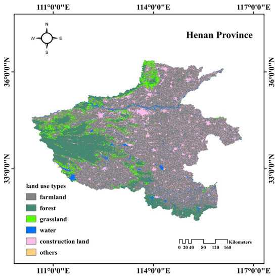
Figure 1.
Land-use-type map in Henan Province, China.
2.2. Data
2.2.1. Global ‘OCO-2’ SIF (GOSIF) Data
A new GOSIF (W m−2 μm−1 sr−1) product with a high spatiotemporal resolution (0.05 degrees, monthly) was developed by Li and Xiao (2019) utilizing the data-driven method. This approach incorporated discrete OCO-2 SIF, MODIS, and meteorological reanalysis data within the predictive SIF model [54]. The GOSIF data can be accessed online at http://globalecology.unh.edu, accessed on 1 January 2023.
2.2.2. Vegetation Index Data
The normalized difference vegetation index (NDVI) is one of the most widely used vegetation indices, which can be calculated from near-infrared and red light bands. Moderate Resolution Imaging Spectroradiometer (MODIS) provides monthly NDVI products with a spatial resolution of 1 km. The monthly NDVI (MOD13A3) data spanning from 2001 to 2020 were downloaded from Google Earth Engine (GEE).
2.2.3. Land Surface Temperature Data
MODIS offers 8-day land surface temperature (LST) products, available for both day and night, with a spatial resolution of 1 km. The MODIS LST-day product (MOD11A2) was downloaded for Henan Province, and the monthly LST results were calculated by the maximum value synthesis method from 2001 to 2020. Similarly, LST data can be obtained from GEE.
2.2.4. Gross Primary Productivity Data
To facilitate a comparison between the downscaled SIF result and GOSIF data, 8-day gross primary productivity (GPP) data (MOD17A2H) with 500 m resolution were obtained. These data will be used for the correlation analysis involving both the downscaled SIF result and GOSIF.
2.2.5. Land-Use Data
The land-use data with a spatial resolution of 1 km used in this study were obtained from the Resource and Environment Science and Data Center (http://www.resdc.cn/, accessed on 1 May 2023). The land-use types identified include farmland, forest, grassland, water, impervious, and others, as depicted in Figure 1.
2.2.6. Statistical Data
The annual areas affected by drought and annual regional level yield (wheat and maize) data were obtained from the National Bureau of Statistics of the People’s Republic of China (http://www.stats.gov.cn/, accessed on 1 May 2023). These drought-affected area figures are instrumental in characterizing the extent of drought impact. Furthermore, the yield data serve as a more appropriate metric for assessing the effects of drought on agriculture. Table 1 summarizes the data used in this study.

Table 1.
Dataset used in this study.
3. Method
SIF, when derived from satellites, has emerged as a potent proxy for photosynthesis on a global scale [57]. SIF with a high spatial resolution is more suitable for regional estimation of the carbon cycle and GPP. Consequently, the RF-based downscaling method was initially used to obtain SIF data with 1 km resolution. Subsequently, the SIF anomaly index was calculated using these downscaled SIF results. Finally, the drought condition was assessed using an SIF anomaly index from 2001 to 2020. Figure 2 describes the specific process including data preparation and processing, the RF method, verification of downscaled SIF result, calculation of the SIF anomaly index, verification of drought index, and the monitoring of drought from 2001 to 2020.
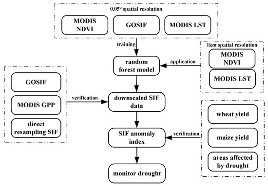
Figure 2.
The flowchart of this study.
3.1. Data Preparation and Processing
The MODIS LST-day data were 8-day composite products. To derive monthly data for the period from 2001 to 2020, the maximum value composite method was employed. Ultimately, both the NDVI and LST-day data were resampled to a resolution of 0.05 degrees using the nearest neighbour method to align with the resolution of the GOSIF.
3.2. RF-Based Downscaled Approach
The RF method is a machine learning model proposed by Breiman in 2001 [58]. This method enhances the decision tree algorithm and is applicable in regression analyses.
In this study, the RF regression model was trained using the sample data of SIF, NDVI, and LST, all at a spatial resolution of 0.05 degrees. The input variables of the model were NDVI and LST, and the predictor variable was SIF. The RF divided input data into many regression trees, making up the forest, where each tree was built from a bootstrap sample. Moreover, a regression model was established for each subset. The average of the prediction results of each regression tree was used as the final prediction result of the model. In the RF method, two parameters—‘ntree’ and ‘mtry’—must be carefully selected based on the sample data. For this study, ‘ntree’ and ‘mtry’ were set at 5 and 2000, respectively.
3.3. Verify Downscaled Result
To evaluate the correlation between the downscaled SIF result and GOSIF, the downscaled results were resampled back to a 0.05-degree spatial resolution. To assess the accuracy of downscaled SIF data, this study calculated the correlation between GOSIF, downscaled SIF and MODIS GPP. Furthermore, to reveal the advantages of the RF method, the direct resampling (nearest neighbour and bilinear) results were used as comparisons with the downscaled SIF result based on the RF method.
3.4. Calculate SIF Anomaly Index
SIF data from 2001 to 2020 were selected; long-time series data are beneficial for monitoring drought. Firstly, the mean SIF for each year is calculated.
where represents the average value of SIF. n equals 12, representing the whole year.
Then, the overall mean SIF from 2001 to 2020 is calculated.
where is the 20-year average of SIF, n is 20.
Finally, is calculated using the following equation:
where is the SIF anomaly index for the i year.
After calculating the SIF anomaly index, the SIF anomaly index image was masked and cropped based on the administrative map of Henan Province in the study area. Simultaneously, the regional average of the SIF anomaly index for the current year was computed as the mean value across all pixels in the image. The spatiotemporal variation in drought in Henan Province from 2001 to 2020 was analysed based on the SIF anomaly index.
3.5. Verify Drought Index
To verify the SIF anomaly index, the Pearson correlation coefficient (R) was computed between the SIF anomaly index and statistical data. The correlation coefficient was calculated using the following formula:
where R is the correlation coefficient, n is the length of the time series, x is the monthly average SIF anomaly index value, y is the value of statistical data in Henan Province, respectively.
3.6. Monitor and Analysis Drought
This study used the SIF anomaly index to monitor the drought in Henan Province. Based on the SIF anomaly index, the long-term drought was analysed in Henan Province from 2001 to 2020.
4. Results
4.1. Spatiotemporal Distribution of Downscaled SIF
The RF-based method was employed to obtain the downscaled SIF data with a resolution of 1 km in Henan Province. Figure 3 provides a detailed illustration of the specific results for May 2018, serving as an example.
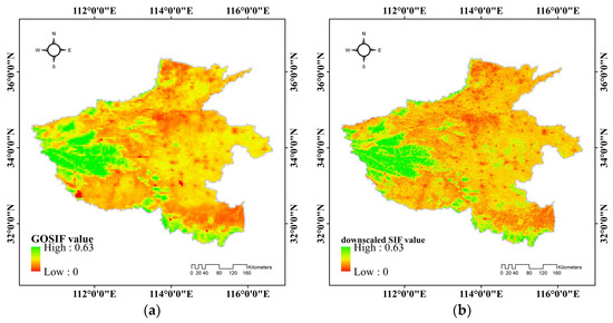
Figure 3.
The GOSIF (W m−2 μm−1 sr−1) and downscaled SIF (W m−2 μm−1 sr−1) result in May 2018. (a) The GOSIF value; (b) the downscaled SIF value based on the RF method.
In Figure 3, the SIF data at different resolutions were compared (GOSIF at 0.05 degrees and downscaled SIF at 1 km). High and low SIF values (W m−2 μm−1 sr−1) were represented by red and green colors, respectively. Relatively high SIF values were predominantly observed in forest areas, followed by grassland and farmland. The comparison figures revealed that the values of the downscaled SIF result had a similar trend to the original GOSIF data. However, the 1 km spatial resolution SIF result could provide more detailed ground information than the 0.05-degree resolution data.
4.2. Verify the Downscaled SIF Result
4.2.1. Correlation Analyses between Downscaled SIF and GOSIF
The downscaled SIF results were resampled to the same spatial resolution (0.05 degrees) as the GOSIF data using the pixel aggregate resampling method. The scatter diagram of the GOSIF and resampled downscaled SIF were obtained (Figure 4). Additionally, the correlation coefficients (R) between downscaled SIF and GOSIF were calculated. The downscaled SIF data exhibited a strong correlation with GOSIF, with a correlation coefficient of 0.74. The distribution of the downscaled SIF and GOSIF data points was observed to be close to the 1:1 line. The high correlation implies that the downscaled SIF effectively preserves the essential information from the original GOSIF products.
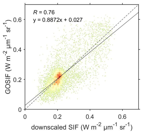
Figure 4.
The scatter diagram of the GOSIF (W m−2 μm−1 sr−1) and resampled downscaled SIF (W m−2 μm−1 sr−1) (the black line denotes the fitting).
4.2.2. Correlation Analyses between SIF and MODIS GPP
Numerous studies have established a linear relationship between SIF (W m−2 μm−1 sr−1) and GPP (g C m−2 a−1) [43,59,60,61,62]. To verify the accuracy of the result, the MOD17A2H GPP product was selected. The MODIS GPP data were obtained by the maximum value synthesis method in May 2018 using 8-day products. The MODIS GPP was resampled to both 1 km and 0.05-degree spatial resolution using the pixel aggregate resampling method. The correlations between MODIS GPP, downscaled SIF, and GOSIF were subsequently calculated (Figure 5).
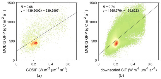
Figure 5.
The correlations among the value of GOSIF (W m−2 μm−1 sr−1), downscaled SIF (W m−2 μm−1 sr−1) and MODIS GPP (g C m−2 a−1) (the black line denotes the fitting). (a) GOSIF and MODIS GPP; (b) downscaled SIF and MODIS GPP.
Figure 5 compares the correlations among the value of GOSIF, downscaled SIF and MODIS GPP. The correlation coefficients (R) at different spatial resolutions were 0.68 and 0.74, respectively. The MODIS GPP and downscaled SIF result (R = 0.74) showed a stronger correlation than GOSIF (R = 0.68). This finding substantiates the credibility of the downscaled results.
4.3. Compare the Downscaled SIF with Direct Resampling Results
To demonstrate the superiority of the RF-based downscaled method, this study conducted a comparison between the downscaled SIF and direct resampling results (Figure 6). GOSIF was resampled to 1 km resolution using nearest neighbour and bilinear methods. The RF-based downscaled, nearest neighbour and bilinear methods SIF results had a similar change trend to the original GOSIF data. The nearest neighbour resampling method significantly altered the texture information of the original image. The bilinear method resulted in smoother images but introduced modifications to the pixel values. The RF algorithm exhibited remarkable robustness against adverse factors, such as noise and outliers. Moreover, it possessed the capability to handle both discrete and continuous data effortlessly, eliminating the necessity for dataset standardization. In contrast, the downscaled SIF result obtained through the RF method exhibited more spatial details compared to the direct resampling methods.
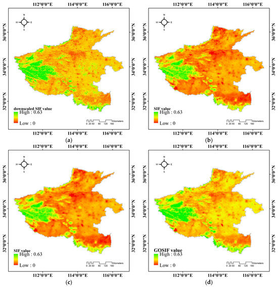
Figure 6.
The SIF (W m−2 μm−1 sr−1) results using RF, nearest neighbour, and bilinear methods. (a) RF-based method, (b) nearest neighbour method, (c) bilinear method, (d) GOSIF.
4.4. Verify the SIF Anomaly Index
4.4.1. Correlation Analyses between Drought Index and Yield
The response of different crops to drought has significant differences. In Henan Province, winter wheat and summer maize are the primary crops. Figure 7 shows the yield changes in wheat and maize in Henan Province. This study aimed to verify the 1 km spatial resolution SIF anomaly index by analysing the response of winter wheat and summer maize yields to drought.
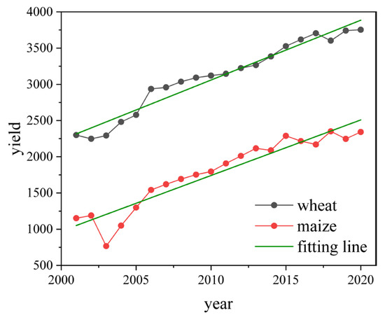
Figure 7.
The yield changes in wheat and maize in Henan Province.
The occurrence of drought in Henan Province exerts an impact on crop growth, consequently influencing crop yield. The SIF anomaly index values in Henan Province were averaged to represent the regional drought index value. Figure 8 illustrates the correlation between the average SIF anomaly value and crop yield from 2001 to 2021. In Henan Province, the SIF anomaly index has positive correlations with crop yield and the scattered points show a statistically significant correlation (p-value < 0.01). The correlation coefficients are 0.93 for wheat and 0.89 for maize, respectively. These high correlations between SIF and crop yields confirm that the SIF anomaly index is a feasible and effective tool for monitoring drought.
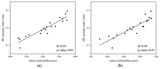
Figure 8.
The correlations among the value of the SIF anomaly index and crop yield (black line is fitting line). (a) SIF index and wheat yield; (b) SIF index and maize yield.
4.4.2. Correlation Analyses between Drought Index and Areas Covered by Drought
The areas affected by drought serve as a direct manifestation in the field of drought. The areas affected by drought are displayed by statistical data which can characterize the extent of the impact of drought. The drought-affected crop area is more appropriate to assess the drought effect in Henan Province. This study utilized data on drought-affected areas in Henan Province, obtained from the National Bureau of Statistics. Due to the unavailability of data for certain years, the study selected data from two periods: 2001 to 2014 and 2014 to 2019. The average SIF anomaly index values with 1 km spatial resolution were obtained by averaging the pixel values of the whole image. Figure 9 illustrates the correlation between the average SIF anomaly index value and areas affected by drought. The results indicated that the index had negative correlations with areas affected by drought, with a correlation coefficient of −0.58. This negative correlation between the drought index and the affected areas demonstrates that the SIF anomaly index is an excellent tool for monitoring drought.
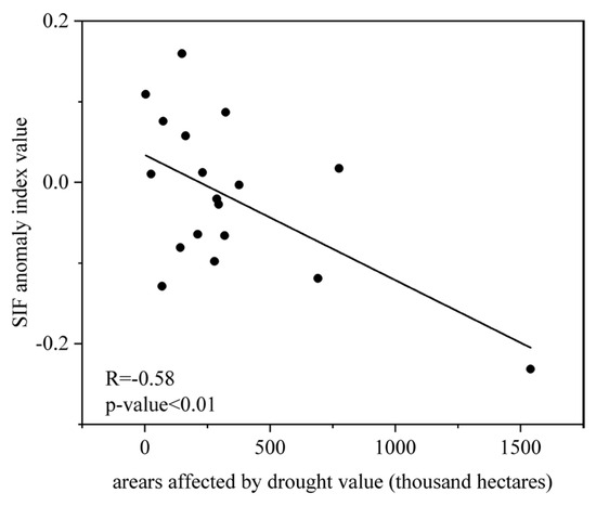
Figure 9.
The correlation of values of the SIF anomaly index and areas affected by drought (black line is fitting line).
4.5. Monitor and Analysis Drought from 2001 to 2020
The determination of drought thresholds has consistently posed challenging research; this study employed the quartile method for drought classification. Upon calculation, an SIF anomaly > 0.087 indicated no drought, normal precipitation, moist soil, and regular growth of vegetation crops without significant drought conditions. When 0.007 < SIF anomaly < 0.087, this suggested mild drought with slightly reduced precipitation and soil moisture levels, exerting a minor impact on vegetation and crops. In the range of −0.081 < SIF anomaly < 0.007, moderate drought is indicated by decreased precipitation and dry soil with insufficient moisture content, leading to notable drought conditions significantly affecting vegetation and crop growth. An SIF anomaly < −0.087 signified severe drought characterized by a substantial reduction in precipitation and severe deficiency in soil moisture, resulting in wilting and a diminished yield of vegetation crops. Figure 10 shows the spatial distribution of drought in Henan Province from 2001 to 2020.
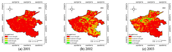
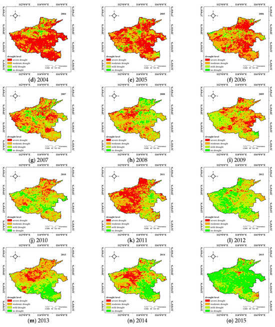
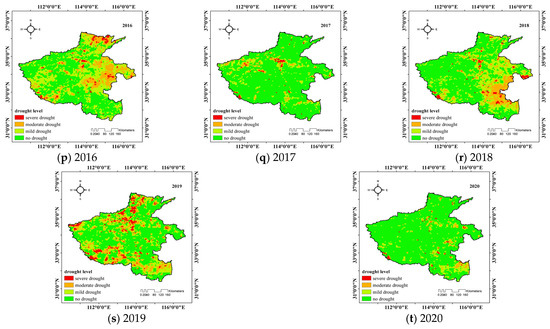
Figure 10.
The spatial distribution of drought in Henan Province from 2001 to 2020.
To monitor and analysis drought, the pixel values of Henan Province were averaged over the period from 2001 to 2020. In this study, a lower SIF anomaly index value indicates more severe drought conditions, and vice versa. As illustrated in Figure 11, the drought situation in Henan Province had been fluctuating up and down over the past 20 years, with a general trend of weakening over time.
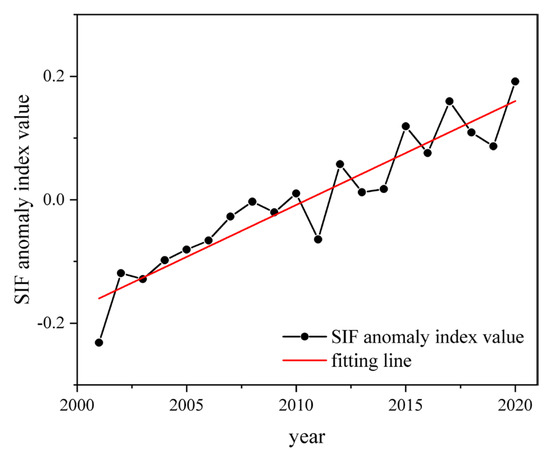
Figure 11.
The change in SIF anomaly index from 2001 to 2020.
5. Discussion
To increase the capacity of managing drought and reducing the adverse effects, timely and effective drought monitoring is indispensable in agricultural management. This study improved the spatial resolution of SIF to 1 km and explored the potential of downscaled SIF in drought detection. Some important and interesting discoveries are discussed in this section.
5.1. Reliability of Downscaled SIF
Since the RF algorithm introduction, it has garnered significant acclaim and found extensive applications across diverse domains [63,64]. Noted for its remarkable predictive accuracy, efficient training speed, and robustness, RF stands out as a preferred option for analysing and optimising models. Therefore, this study utilized the RF approach to build the downscaled SIF model.
The relationship between SIF and GPP has been consistently demonstrated in previous studies [2]. In this study, the downscaled SIF exhibited a stronger positive correlation with MODIS GPP compared to GOSIF, with correlation coefficients of 0.74 and 0.68, respectively (Figure 5). This finding further validates the reliability of the downscaled results. Meanwhile, to demonstrate the superiority of the RF-based downscaled method, this study conducted a comparative analysis between the downscaled SIF and direct resampling results (Figure 6). The downscaled SIF result obtained through the RF method exhibited enhanced spatial resolution compared to that achieved by direct resampling methods. The downscaled SIF not only preserves the information of the original GOSIF, but more significantly enhances spatial resolution through the research conducted.
5.2. The Ability of SIF Anomaly to Monitor Drought
SIF is closely associated with vegetation photosynthesis and can serve as a valuable tool for monitoring the physiological status of vegetation and water stress conditions [65]. During drought events, water stress induces alterations in the physiological state of vegetation, consequently leading to changes in SIF [66]. In this study, we validated the applicability of SIF for drought monitoring using various approaches such as MODIS GPP, crop yield, and drought-affected areas. By establishing an SIF-based drought index, we successfully monitored drought occurrences in Henan Province.
The occurrence of drought will exert an impact on crop growth, ultimately leading to a decrease in crop yield [13]. The SIF anomaly value had positive correlations with wheat and maize yield (Figure 8). The correlation coefficients were 0.93 and 0.89. Meanwhile, the SIF anomaly value had negative correlations with areas affected by drought, with a correlation coefficient of −0.58 (Figure 9). The SIF anomaly index had a high correlation with the factors that characterized drought. It indicated that the SIF anomaly index was a useful factor for characterizing drought. Therefore, our study presents an alternative data source and selectable index for future regional drought monitoring and analysis.
5.3. Advantages of Downscaled SIF in Drought Monitoring
The current limitations of satellite technology pose a challenge in achieving high temporal and spatial resolutions simultaneously in existing satellite SIF products [67]. These coarse-resolution downscaled SIF data (0.05 degrees) present challenges for various research fields, including regional carbon cycle, crop growth studies, and drought assessments [2,66,68]. High spatial resolution satellite data are more suitable for regional agricultural drought monitoring. For instance, the spatial resolution of MODIS products has reached 1 km and 500 m, providing an advantage in regional drought monitoring [69,70]. Moreover, the fragmentation of farmland in China is highly pronounced and low-resolution SIF products are insufficient for accurate regional agricultural drought monitoring. Therefore, the demand for higher resolution SIF products is urgent in order to achieve accurate regional drought monitoring and assessments. In this study, a lower SIF anomaly index value indicates more severe drought conditions while vice versa holds true. The downscaled SIF results (1 km spatial resolution) have been successfully applied to monitor drought in Henan Province (Figure 10 and Figure 11). Henceforth, the downscaled 1 km spatial resolution SIF results presented in this study offer significant advantages for regional drought monitoring.
5.4. The Limitations of This Study
However, there are also inherent limitations in this research. Firstly, the input parameters of the downscaling model only included MODIS NDVI and LST data, without incorporating meteorological and soil condition data. In future research, it is imperative to assess the influence of different input parameters on the model’s output results. Secondly, drought is a complex phenomenon influenced by various interconnected factors encompassing the atmosphere, vegetation, and soil. Consequently, it becomes imperative to integrate multi-source remote sensing data while modelling drought and establishing indices. Lastly, for effective drought monitoring in China where farmland often exhibits a fragmented state, higher resolution remote sensing products are indispensable.
6. Conclusions
This study, conducted in Henan Province, China, utilized the RF-based downscaling method to enhance the spatial resolution of GOSIF data from 0.05 degrees to 1 km. GOSIF, NDVI, and LST with 0.05-degree spatial resolution were used as sample data to train the RF regression model. NDVI and LST were the input variables, with SIF as the predictor. Using the downscaled SIF result, the SIF anomaly index was calculated. Crop yield and areas affected by drought were selected to verify the drought index. Finally, the SIF anomaly index was used to monitor drought in Henan Province.
The downscaled SIF result exhibited a higher correlation with MODIS GPP data than the 0.05-degree GOSIF, with correlation coefficients of 0.74 and 0.68, respectively. After resampling the downscaled SIF to a 0.05-degree resolution to match the GOSIF, a strong correlation was still observed. To show the superiority of the RF method, this study compared the downscaled SIF with direct resampling methods (nearest neighbour and bilinear). The results indicated that the downscaled SIF result showed enhanced spatial details, which was significant to study and monitor the regional GPP in Henan Province. Using the 1 km spatial resolution, the SIF anomaly index was established and calculated. Utilizing the 1 km resolution, the SIF anomaly index established strong positive correlations with crop yields (0.93 for wheat and 0.89 for maize), and a significant negative correlation with drought-affected areas (−0.58). The SIF anomaly index, based on the 1 km resolution downscaled SIF data using the RF method, proved to be a valuable tool for studying regional drought. Furthermore, the SIF anomaly index also presented researchers with a novel alternative for future drought monitoring. The findings presented in this research offer robust and scientifically sound data support for drought monitoring in Henan Province.
Author Contributions
Conceptualization, Z.Z.; methodology, Z.Z. and Z.G.; validation, Z.Z. and X.L.; formal analysis, Z.Z. and Y.Q.; investigation, X.L.; data curation, Z.S.; funding acquisition, Y.J.; writing—original draft preparation, Z.Z. and Z.S.; writing—review and editing, Z.Z. and Y.J. All authors have read and agreed to the published version of the manuscript.
Funding
This research was funded by Key R&D Program of Shandong Province (2022CXGC020416).
Data Availability Statement
Data are contained within the article.
Acknowledgments
We thank the MODIS and land-used products. Meanwhile, we are very grateful for Jingfeng Xiao and Xing Li who provided GOSIF data for this paper.
Conflicts of Interest
The authors declare no conflicts of interest.
References
- Diffenbaugh, N.S.; Pal, J.S.; Trapp, R.J.; Giorgi, F. Fine-Scale Processes Regulate the Response of Extreme Events to Global Climate Change. Proc. Natl. Acad. Sci. USA 2005, 102, 15774–15778. [Google Scholar] [CrossRef]
- Zhang, Z.; Xu, W.; Qin, Q.; Long, Z. Downscaling Solar-Induced Chlorophyll Fluorescence Based on Convolutional Neural Network Method to Monitor Agricultural Drought. IEEE Trans. Geosci. Remote Sens. 2020, 59, 1012–1028. [Google Scholar] [CrossRef]
- Keyantash, J.; Dracup, J.A. The Quantification of Drought: An Evaluation of Drought Indices. Bull. Am. Meteorol. Soc. 2002, 1167–1180. [Google Scholar] [CrossRef]
- Wilhite, D.A. Drought as a Natural Hazard: Concepts and Definitions. Drought A Glob. Assess. 2000, I, 3–18. [Google Scholar]
- Svoboda, M.; LeComte, D.; Hayes, M.; Heim, R.; Gleason, K.; Angel, J.; Rippey, B.; Tinker, R.; Palecki, M.; Stooksbury, D.; et al. The Drought Monitor. Bull. Am. Meteorol. Soc. 2002, 83, 1181–1190. [Google Scholar] [CrossRef]
- Dai, A. Drought under Global Warming: A Review. Wiley Interdiscip. Rev. Clim. Chang. 2011, 2, 45–65. [Google Scholar] [CrossRef]
- Tucker, C.J.; Choudhury, B.J. Choudhury Satellite Remote Sensing of Drought Conditions. Remote Sens. Environ. 1987, 23, 243–251. [Google Scholar] [CrossRef]
- Wilhite, D.A.; Glantz, M.H. Understanding: The Drought Phenomenon: The Role of Definitions. Water Int. 1985, 10, 111–120. [Google Scholar] [CrossRef]
- Heim, R.R., Jr. A Review of Twentieth-Century Drought Indices Used in the United States. Bull. Am. Meteorol. Soc. 2002, 83, 1149–1166. [Google Scholar] [CrossRef]
- Wei, W.; Zhang, J.; Zhou, J.; Zhou, L.; Li, C. Monitoring Drought Dynamics in China Using Optimized Meteorological Drought Index (OMDI) Based on Remote Sensing Data Sets. J. Environ. Manag. 2021, 292, 112733. [Google Scholar] [CrossRef]
- Zhao, H.; Xu, Z.; Zhao, J.; Huang, W. A drought rarity and evapotranspiration-based index as a suitable agricultural drought indicator. Ecol. Indic. 2017, 82, 530–538. [Google Scholar] [CrossRef]
- Cheng, T.; Hong, S.; Huang, B.; Tan, C. Passive Microwave Remote Sensing Soil Moisture Data in Agricultural Drought Monitoring: Application in Northeastern China. Water 2021, 13, 2777. [Google Scholar] [CrossRef]
- Qin, Q.; Wu, Z.; Zhang, T.; Sagan, V.; Zhang, Z.; Zhang, Y.; Zhang, C.; Ren, H.; Sun, Y.; Xu, W.; et al. Optical and Thermal Remote Sensing for Monitoring Agricultural Drought. Remote Sens. 2021, 13, 5092. [Google Scholar] [CrossRef]
- AghaKouchak, A.; Farahmand, A.; Melton, F.; Teixeira, J.; Anderson, M.; Wardlow, B.D.; Hain, C. Remote Sensing of Drought: Progress, Challenges and Opportunities. Rev. Geophys. 2015, 53, 452–480. [Google Scholar] [CrossRef]
- Kim, Y.; Lee, S.B.; Yun, H.; Kim, J.; Park, Y. A Drought Analysis Method Based on Modis Satellite Imagery and AWS Data. In Proceedings of the Geoscience & Remote Sensing Symposium, Fort Worth, TX, USA, 23–28 July 2017. [Google Scholar]
- McKee, T.B.; Doesken, N.J.; Kleist, J.; Kleist, J. The Relationship of Drought Frequency and Duration to Time Scales. In Proceedings of the 8th Conference on Applied Climatology, American Meteorological Society, Boston, MA, USA, 17–22 January 1993; Volume 17, pp. 179–183. [Google Scholar]
- Vicente-Serrano, S.M.; Beguería, S.; López-Moreno, J.I. A Multiscalar Drought Index Sensitive to Global Warming: The Standardized Precipitation Evapotranspiration Index. J. Clim. 2010, 23, 1696–1718. [Google Scholar] [CrossRef]
- Palmer, W.C. Meteorological Drought; Research Paper No. 45; US Department of Commerce, Weather Bureau: Washington, DC, USA, 1965; Volume 58.
- Prodhan, F.A.; Zhang, J.; Bai, Y.; Prasad, T.; Koju, U.A. Monitoring of Drought Condition and Risk in Bangladesh Combined Data from Satellite and Ground Meteorological Observations. IEEE Access 2020, 8, 93264–93282. [Google Scholar] [CrossRef]
- Zhang, Z.; Xu, W.; Shi, Z.; Qin, Q. Establishment of a Comprehensive Drought Monitoring Index Based on Multisource Remote Sensing Data and Agricultural Drought Monitoring. IEEE J. Sel. Top. Appl. Earth Obs. Remote Sens. 2021, 14, 2113–2126. [Google Scholar] [CrossRef]
- West, H.; Quinn, N.; Horswell, M. Remote Sensing for Drought Monitoring & Impact Assessment: Progress, Past Challenges and Future Opportunities. Remote Sens. Environ. 2019, 232, 111291. [Google Scholar]
- Rouse, J., Jr.; Haas, R.; Schell, J.; Deering, D. Monitoring Vegetation Systems in the Great Plains with ERTS. NASA Spec. Publ. 1974, 351, 309. [Google Scholar]
- Yang, L.; Wylie, B.K.; Tieszen, L.L.; Reed, B.C. An Analysis of Relationships among Climate Forcing and Time-Integrated NDVI of Grasslands over the US Northern and Central Great Plains. Remote Sens. Environ. 1998, 65, 25–37. [Google Scholar] [CrossRef]
- Kogan, F. Remote Sensing of Weather Impacts on Vegetation in Non-Homogeneous Areas. Int. J. Remote Sens. 1990, 11, 1405–1419. [Google Scholar] [CrossRef]
- Kogan, F.N. Droughts of the Late 1980s in the United States as Derived from NOAA Polar-Orbiting Satellite Data. Bull. Am. Meteorol. Soc. 1995, 76, 655–668. [Google Scholar] [CrossRef]
- Aghakouchak, A. A Baseline Probabilistic Drought Forecasting Framework Using Standardized Soil Moisture Index: Application to the 2012 United States Drought. Hydrol. Earth Syst. Sci. 2014, 18, 2485–2492. [Google Scholar] [CrossRef]
- Zhang, G.A. Jia Monitoring Meteorological Drought in Semiarid Regions Using Multi-Sensor Microwave Remote Sensing Data. Remote Sens. Environ. Interdiscip. J. 2013, 134, 12–23. [Google Scholar] [CrossRef]
- Cao, B. NDWI—A Normalized Difference Water Index for Remote Sensing of Vegetation Liquid Water from Space. Remote Sens. Environ. Interdiscip. J. 1996, 58, 257–266. [Google Scholar]
- Wang, L.; Qu, J.J. NMDI: A Normalized Multi-Band Drought Index for Monitoring Soil and Vegetation Moisture with Satellite Remote Sensing. Geophys. Res. Lett. 2007, 34, 1–5. [Google Scholar] [CrossRef]
- Chen, X.; Mo, X.; Zhang, Y.; Sun, Z.; Liu, Y.; Hu, S.; Liu, S. Drought Detection and Assessment with Solar-Induced Chlorophyll Fluorescence in Summer Maize Growth Period over North China Plain. Ecol. Indic. 2019, 104, 347–356. [Google Scholar] [CrossRef]
- Rhee, J.; Im, J.; Carbone, G.J. Monitoring Agricultural Drought for Arid and Humid Regions Using Multi-Sensor Remote Sensing Data. Remote Sens. Environ. 2010, 114, 2875–2887. [Google Scholar] [CrossRef]
- Hao, C.; Zhang, J.; Yao, F. Combination of Multi-Sensor Remote Sensing Data for Drought Monitoring over Southwest China. Int. J. Appl. Earth Obs. Geoinf. 2015, 35, 270–283. [Google Scholar] [CrossRef]
- McFarlane, J.; Watson, R.D.; Theisen, A.F.; Jackson, R.D.; Ehrler, W.; Pinter, P.; Idso, S.B.; Reginato, R. Plant Stress Detection by Remote Measurement of Fluorescence. Appl. Opt. 1980, 19, 3287–3289. [Google Scholar] [CrossRef] [PubMed]
- Daumard, F.; Champagne, S.; Fournier, A.; Goulas, Y.; Ounis, A.; Hanocq, J.-F.; Moya, I. A Field Platform for Continuous Measurement of Canopy Fluorescence. IEEE Trans. Geosci. Remote Sens. 2010, 48, 3358–3368. [Google Scholar] [CrossRef]
- Grace, J.; Nichol, C.; Disney, M.; Lewis, P.; Quaife, T.; Bowyer, P. Can We Measure Terrestrial Photosynthesis from Space Directly, Using Spectral Reflectance and Fluorescence? Glob. Chang. Biol. 2007, 13, 1484–1497. [Google Scholar] [CrossRef]
- Guanter, L.; Zhang, Y.; Jung, M.; Joiner, J.; Voigt, M.; Berry, J.A.; Frankenberg, C.; Huete, A.R.; Zarco-Tejada, P.; Lee, J.-E.; et al. Global and Time-Resolved Monitoring of Crop Photosynthesis with Chlorophyll Fluorescence. Proc. Natl. Acad. Sci. USA 2014, 111, E1327–E1333. [Google Scholar] [CrossRef] [PubMed]
- Liu, X.; Guanter, L.; Liu, L.; Damm, A.; Malenovskỳ, Z.; Rascher, U.; Peng, D.; Du, S.; Gastellu-Etchegorry, J.-P. Downscaling of Solar-Induced Chlorophyll Fluorescence from Canopy Level to Photosystem Level Using a Random Forest Model. Remote Sens. Environ. 2019, 231, 110772. [Google Scholar] [CrossRef]
- Migliavacca, M.; Perez-Priego, O.; Rossini, M.; El-Madany, T.S.; Moreno, G.; van der Tol, C.; Rascher, U.; Berninger, A.; Bessenbacher, V.; Burkart, A.; et al. Plant Functional Traits and Canopy Structure Control the Relationship between Photosynthetic CO2 Uptake and Far-Red Sun-Induced Fluorescence in a Mediterranean Grassland under Different Nutrient Availability. New Phytol. 2017, 214, 1078–1091. [Google Scholar] [CrossRef] [PubMed]
- Verrelst, J.; van der Tol, C.; Magnani, F.; Sabater, N.; Rivera, J.P.; Mohammed, G.; Moreno, J. Evaluating the Predictive Power of Sun-Induced Chlorophyll Fluorescence to Estimate Net Photosynthesis of Vegetation Canopies: A SCOPE Modeling Study. Remote Sens. Environ. 2016, 176, 139–151. [Google Scholar] [CrossRef]
- Rascher, U.; Kraska, T.; Rossini, M.; Schuettemeyer, D.; Pinto, F.; Hyvärinen, T.; Kraft, S.; Cendrero, P.; Cogliati, S.; Schickling, A. Mapping Sun-Induced Fluorescence (SIF) for Mechanistic Stress Responses of Vegetation Using the High-Performance Imaging Spectrometer HyPlant. In Proceedings of the 9th EARSel Imaging Spectroscopy Workshop, Luxembourg, 14–16 April 2015. [Google Scholar]
- Baker, N.R. Chlorophyll Fluorescence: A Probe of Photosynthesis in Vivo. Annu. Rev. Plant Biol. 2008, 59, 89–113. [Google Scholar] [CrossRef]
- Lichtenthaler, H.; Buschmann, C.; Rinderle, U.; Schmuck, G. Application of Chlorophyll Fluorescence in Ecophysiology. Radiat. Environ. Biophys. 1986, 25, 297–308. [Google Scholar] [CrossRef]
- Frankenberg, C.; Fisher, J.B.; Worden, J.; Badgley, G.; Saatchi, S.S.; Lee, J.-E.; Toon, G.C.; Butz, A.; Jung, M.; Kuze, A.; et al. New Global Observations of the Terrestrial Carbon Cycle from GOSAT: Patterns of Plant Fluorescence with Gross Primary Productivity. Geophys. Res. Lett. 2011, 38, L17706. [Google Scholar] [CrossRef]
- Joiner, J.; Yoshida, Y.; Vasilkov, A.P.; Yoshida, Y.; Corp, L.A.; Middleton, E.M. First Observations of Global and Seasonal Terrestrial Chlorophyll Fluorescence from Space. Biogeosciences 2011, 8, 637–651. [Google Scholar] [CrossRef]
- Joiner, J.; Guanter, L.; Lindstrot, R.; Voigt, M.; Vasilkov, A.; Middleton, E.; Huemmrich, K.; Yoshida, Y.; Frankenberg, C. Global Monitoring of Terrestrial Chlorophyll Fluorescence from Moderate-Spectral-Resolution Near-Infrared Satellite Measurements: Methodology, Simulations, and Application to GOME-2. Atmos. Meas. Tech. 2013, 6, 2803–2823. [Google Scholar] [CrossRef]
- Köhler, P.; Guanter, L.; Joiner, J. A Linear Method for the Retrieval of Sun-Induced Chlorophyll Fluorescence from GOME-2 and SCIAMACHY Data. Atmos. Meas. Tech. 2015, 8, 2589–2608. [Google Scholar] [CrossRef]
- Joiner, J.; Yoshida, Y.; Guanter, L.; Middleton, E.M. New Methods for the Retrieval of Chlorophyll Red Fluorescence from Hyperspectral Satellite Instruments: Simulations and Application to GOME-2 and SCIAMACHY. Atmos. Meas. Tech. 2016, 9, 3939–3967. [Google Scholar] [CrossRef]
- Joiner, J.; Yoshida, Y.; Vasilkov, A.P.; Middleton, E.M.; Campbell, P.K.; Yoshida, Y.; Kuze, A.; Corp, L.A. Filling-in of Far-Red and Near-Infrared Solar Lines by Terrestrial and Atmospheric Effects: Simulations and Space-Based Observations from SCHIAMACHY and GOSAT. Atmos. Meas. Tech. Discuss. 2012, 5, 163–210. [Google Scholar]
- Frankenberg, C.; O’Dell, C.; Berry, J.; Guanter, L.; Joiner, J.; Köhler, P.; Pollock, R.; Taylor, T.E. Prospects for Chlorophyll Fluorescence Remote Sensing from the Orbiting Carbon Observatory-2. Remote Sens. Environ. 2014, 147, 1–12. [Google Scholar] [CrossRef]
- Duveiller, G.; Filipponi, F.; Walther, S.; Köhler, P.; Frankenberg, C.; Guanter, L.; Cescatti, A. A Spatially Downscaled Sun-Induced Fluorescence Global Product for Enhanced Monitoring of Vegetation Productivity. Earth Syst. Sci. Data 2019, 12, 1101–1116. [Google Scholar] [CrossRef]
- Ji, M.; Tang, B.; Li, Z. Review of Solar-Induced Chlorophyll Fluorescence Retrieval Method from Satellite Data. Remote Sens. Technol. Appl. 2019, 34, 455–466. [Google Scholar]
- Duveiller, G.; Cescatti, A. Spatially Downscaling Sun-Induced Chlorophyll Fluorescence Leads to an Improved Temporal Correlation with Gross Primary Productivity. Remote Sens. Environ. 2016, 182, 72–89. [Google Scholar] [CrossRef]
- Gentine, P.; Alemohammad, S. Reconstructed Solar-Induced Fluorescence: A Machine Learning Vegetation Product Based on MODIS Surface Reflectance to Reproduce GOME-2 Solar-Induced Fluorescence. Geophys. Res. Lett. 2018, 45, 3136–3146. [Google Scholar] [CrossRef]
- Li, X.; Xiao, J. A Global, 0.05-Degree Product of Solar-Induced Chlorophyll Fluorescence Derived from OCO-2, MODIS, and Reanalysis Data. Remote Sens. 2019, 11, 517. [Google Scholar] [CrossRef]
- Yu, L.; Wen, J.; Chang, C.; Frankenberg, C.; Sun, Y. High-Resolution Global Contiguous SIF of OCO-2. Geophys. Res. Lett. 2019, 46, 1449–1458. [Google Scholar] [CrossRef]
- Zhang, Y.; Joiner, J.; Alemohammad, S.H.; Zhou, S.; Gentine, P. A Global Spatially Contiguous Solar-Induced Fluorescence (CSIF) Dataset Using Neural Networks. Biogeosciences 2018, 15, 5779–5800. [Google Scholar] [CrossRef]
- Wen, J.; Köhler, P.; Duveiller, G.; Parazoo, N.; Magney, T.; Hooker, G.; Yu, L.; Chang, C.; Sun, Y. A Framework for Harmonizing Multiple Satellite Instruments to Generate a Long-Term Global High Spatial-Resolution Solar-Induced Chlorophyll Fluorescence (SIF). Remote Sens. Environ. 2020, 239, 111644. [Google Scholar] [CrossRef]
- Breiman, L. Random Forests. Mach. Learn. 2001, 45, 5–32. [Google Scholar] [CrossRef]
- Guanter, L.; Frankenberg, C.; Dudhia, A.; Lewis, P.E.; Gómez-Dans, J.; Kuze, A.; Suto, H.; Grainger, R.G. Retrieval and Global Assessment of Terrestrial Chlorophyll Fluorescence from GOSAT Space Measurements. Remote Sens. Environ. 2012, 121, 236–251. [Google Scholar] [CrossRef]
- Sanders, A.; Verstraeten, W.; Kooreman, M.; Van Leth, T.; Beringer, J.; Joiner, J. Spaceborne Sun-Induced Vegetation Fluorescence Time Series from 2007 to 2015 Evaluated with Australian Flux Tower Measurements. Remote Sens. 2016, 8, 895. [Google Scholar] [CrossRef]
- Sun, Y.; Frankenberg, C.; Jung, M.; Joiner, J.; Guanter, L.; Köhler, P.; Magney, T. Overview of Solar-Induced Chlorophyll Fluorescence (SIF) from the Orbiting Carbon Observatory-2: Retrieval, Cross-Mission Comparison, and Global Monitoring for GPP. Remote Sens. Environ. 2018, 209, 808–823. [Google Scholar] [CrossRef]
- Wagle, P.; Zhang, Y.; Jin, C.; Xiao, X. Comparison of Solar-Induced Chlorophyll Fluorescence, Light-Use Efficiency, and Process-Based GPP Models in Maize. Ecol. Appl. 2016, 26, 1211–1222. [Google Scholar] [CrossRef]
- Fawagreh, K.; Gaber, M.M.; Elyan, E. Random Forests: From Early Developments to Recent Advancements. Syst. Sci. Control Eng. Open Access J. 2014, 2, 602–609. [Google Scholar] [CrossRef]
- Abdulkareem, N.M.; Abdulazeez, A.M. Machine Learning Classification Based on Radom Forest Algorithm: A Review. Int. J. Sci. Bus. 2021, 5, 128–142. [Google Scholar]
- Xu, S.; Atherton, J.; Riikonen, A.; Zhang, C.; Oivukkamäki, J.; MacArthur, A.; Honkavaara, E.; Hakala, T.; Koivumäki, N.; Liu, Z.; et al. Structural and Photosynthetic Dynamics Mediate the Response of SIF to Water Stress in a Potato Crop. Remote Sens. Environ. 2021, 263, 112555. [Google Scholar] [CrossRef]
- Geng, G.; Yang, R.; Liu, L. Downscaled Solar-Induced Chlorophyll Fluorescence Has Great Potential for Monitoring the Response of Vegetation to Drought in the Yellow River Basin, China: Insights from an Extreme Event. Ecol. Indic. 2022, 138, 108801. [Google Scholar] [CrossRef]
- Bacour, C.; Maignan, F.; Peylin, P.; Macbean, N.; Bastrikov, V.; Joiner, J.; Köhler, P.; Guanter, L.; Frankenberg, C. Differences Between OCO-2 and GOME-2 SIF Products from a Model-Data Fusion Perspective. J. Geophys. Res. Biogeosci. 2019, 124, 3143–3157. [Google Scholar] [CrossRef]
- Whelan, M.E.; Anderegg, L.D.L.; Badgley, G.; Campbell, J.E.; Commane, R.; Frankenberg, C.; Hilton, T.W.; Kuai, L.; Parazoo, N.; Shiga, Y. Two Scientific Communities Striving for a Common Cause: Innovations in Carbon Cycle Science. Bull. Am. Meteorol. Soc. 2020, 101, E1537–E1543. [Google Scholar] [CrossRef]
- Ma, Z.C.; Sun, P.; Zhang, Q.; Hu, Y.Q.; Jiang, W. Characterization and Evaluation of MODIS-Derived Crop Water Stress Index (CWSI) for Monitoring Drought from 2001 to 2017 over Inner Mongolia. Sustainability 2021, 13, 916. [Google Scholar] [CrossRef]
- Tao, L.; Ryu, D.; Western, A.; Boyd, D. A New Drought Index for Soil Moisture Monitoring Based on MPDI-NDVI Trapezoid Space Using MODIS Data. Remote Sens. 2020, 13, 122. [Google Scholar] [CrossRef]
Disclaimer/Publisher’s Note: The statements, opinions and data contained in all publications are solely those of the individual author(s) and contributor(s) and not of MDPI and/or the editor(s). MDPI and/or the editor(s) disclaim responsibility for any injury to people or property resulting from any ideas, methods, instructions or products referred to in the content. |
© 2024 by the authors. Licensee MDPI, Basel, Switzerland. This article is an open access article distributed under the terms and conditions of the Creative Commons Attribution (CC BY) license (https://creativecommons.org/licenses/by/4.0/).