Abstract
Analysis of a series of thermal mappings obtained by UAS flights on quiescent volcanoes requires some special techniques to be performed. The main challenge is represented by the difficulty of separating hot and cold pixels in areas where their temperatures are quite similar. This task is indeed much simpler, for example, for lava flows where the temperature differences between the hot lava and the cold soil is rather big. This paper shows various software developed in order to perform this extraction and calculate the trends over time of both the average temperature and the heat flux from the soil. This prototypal implementation used thermal flights performed over a time span of a few years on an area in the Campi Flegrei caldera in southern Italy. Standard image manipulation techniques were used to segmentate and clusterise each thermal mapping in order to reduce the thermal anomalies to some sets of simpler features characterised by their fundamental parameters. The temporal trends of some physical parameters (temperature, heat flux, etc.) were extracted from these sets, and we found interesting results necessary for correlations and for ongoing research with other parameters.
1. Introduction
Thermal energy release in active geothermal areas is a key parameter to evaluate the dynamics of the underlying geological background. In particular, in a volcanic context, it provides a fundamental contribution to the knowledge of volcanic processes and may be used to evaluate the related hazards and aid risk management ([1] and references therein).
Validated heat flux measurement procedures from the literature, based on measuring thermal gradient [1,2,3,4,5,6,7] or carbon dioxide flux [8,9], only allow for punctual measurements and require physical access to the sites in order to be performed. These kinds of measurements require extensive time to be fulfilled: they may take days or even weeks to be completed, even in the case of small areas (few km2 or less) like La Solfatara crater or Pisciarelli crater in Campi Flegrei caldera in Italy [10,11,12]. A new method has been developed and validated [13] in La Solfatara crater based on measuring ground temperature with a thermal camera on a tripod and repeating the measures on hundreds of points of the crater in different seasons for a period of 5 years. Similar to the classic methods, this one suffers from the need to take lots of thermal pictures in order to cover the required area. Furthermore, this method does not solve the timing issue of the classical punctual methods, but it opened the way to new ideas to use the ground temperature as a proxy for the heat flux.
The use of a UAS to capture thermal images solves the timing issue of the punctual methods as even a rather large area can be scanned in a matter of minutes. Programs used to create the mosaics from the single thermal images are reliable as the errors introduced by the interpolation algorithms are negligible compared to the temperature error of the thermal camera used [14,15]. This paper presents a prototype software created to analyse a time series of mosaics of thermal images shot from UAS in order to calculate the flux of energy in a way similar to what was done in Cirillo et al. 2022a, 2022b [16,17].
The presented software applies to the thermal mosaic the same algorithms (KMEANS and DBSCAN) used in Cirillo et al. 2022 (references therein [16]) to separate cold and hot areas into single thermal images. Once the hot areas are separated from the background, and the background temperature has been estimated, it applies the heat transfer model developed in Marotta et al. 2019 [13] and stores the result of the clusterisation for further analysis. The clusters obtained are then grouped using another program which uses the DBSCAN algorithm again to gather them into homogeneous zones, keeping their time information, which are then used to create the time evolution of the desired parameters.
All the software developed to perform the present analyses is available as Supplementary Materials in a Zenodo repository.
2. Materials and Methods
The research was carried out in the Pisciarelli area which has the same physical characteristics as the soil of the La Solfatara crater [11], where the heat flux model described in Marotta et al. 2019 was developed (Figure 1).
From 2019 to nowadays, UAS flights have been executed monthly in the Pisciarelli area during the evening and/or night, in any case, always in absence of solar irradiation. The flights were performed using a thermal camera FLIR Vue Pro R (technical details are in Silvestri et al., 2020 [18] and in Caputo et al. 2023 [14]).
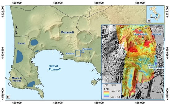
Figure 1.
(a) Study area. (b) The blue squares highlight the Solfatara crater and Pisciarelli area. Digital terrain model (DTM) of Campi Flegrei [19]. (c) Radiometric mapping of the entire Pisciarelli area. DSM from mosaic of data SIT Città Metropolitana di Napoli.
During the aforementioned period, about 40 radiometric mosaics were produced, some of which were obtained by combining two different flight plans with different take-off and landing points (shown in Figure 2 as “Home Concessionaria” and “Home Elipista”). Most of the mosaics were obtained with a single flight having as take-off and landing point the “Home Elipista’’ point in Figure 1, which also shows an example of a radiometric mapping of the entire Pisciarelli area.
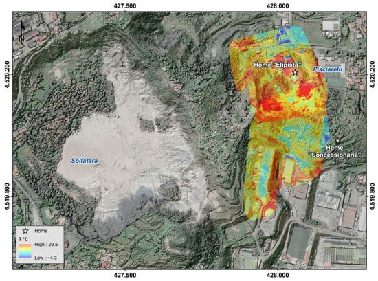
Figure 2.
Radiometric mapping of the Pisciarelli area by overlapping 343 thermal images using specific software (Analist and Pix4D Mapper [20,21]). “Home Elipista” and “Home Concessionaria” with its take-off and landing point are shown in the figure. Source: Esri, Maxar, Earthstar Geographics, and the GIS User Community. DSM from mosaic of data SIT Città Metropolitana di Napoli.
Flight plans were adjusted during the acquisition period to find the best parameters related to the equipment used in order to adapt them to the complex topography of the selected area. After this test period, a flight quote between 70 and 55 m agl (above ground levels) was decided to be used, following the morphology of the terrain with the camera in a nadiral position and using a single grid for each flight (Figure 3). Total number of images taken and ground sampling distance change with the flight height. Flying at about 120 m, the pixel resolution is of about 25 cm2 and requires a few tens of images, while a flight at about 55 m has a pixel resolution of about 10 cm2 and requires hundreds of images. We used the same image superposition for all the performed flights: 80% front overlap and 60% side overlap between adjacent image footprints in width and height. The internal firmware of the FLIR thermal camera allowed correction for distance, relative humidity, air temperature, and soil emissivity, which are constant for the whole flight as they can only be set before take-off. Soil emissivity is set to 0.98 according to Flynn et al. 1993 [22] and Pinkerton et al. 2002 [23]. We can assume such emissivity value for thermally anomalous zones as they are made of quite uniform material. In any case, the angle of view at which the single images are taken may introduce undecidable errors as it is not possible to always know the real angle of the camera in relation to the terrain [24,25,26].
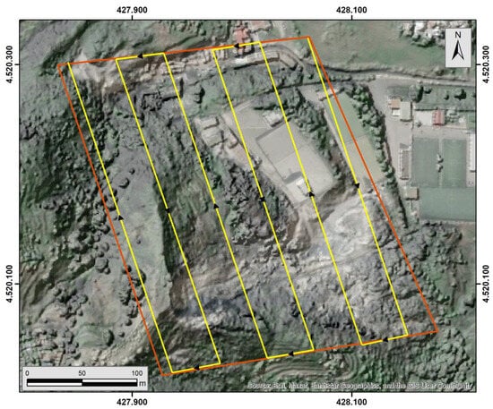
Figure 3.
Example of flight plans in Pisciarelli: simple grid. Source: Esri, Maxar, Earthstar Geographics, and GIS User Community. DSM from mosaic of data SIT Città Metropolitana di Napoli.
Figure 4 shows a zoom of the area with the biggest thermal anomalies together with a visible mapping. All the thermal maps have been exported from the ArcGis Environment [27], selecting only the radiometric component in ASCII GRID format file to improve data readability.
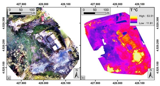
Figure 4.
(a) Visible and (b) thermal mapping of Pisciarelli area (blue square in Figure 1) with drone take-off point from “Home Elipista”.
2.1. Clustering of Thermal Mappings
To determine the amount of energy emitted from the ground (thermal flux), the hot zones need to be separated from the cold ones. Unfortunately, a valid threshold for all the flights cannot be applied in a straightforward way because the temperature difference between warm areas and cold ones is not big enough and the temperature distribution of the pixels depends on the season and on the external temperature, despite nightly acquisitions.
A more complex algorithm needed to be implemented to achieve such separation considering that it is important to extract both warm and cold areas, with the latter necessary to establish the background temperature (BG) which is an essential parameter of the Solfatara model [13]. The BG must relate to an area, even just a few m2, where the ground has similar physical properties of those with temperature anomalies: it is important to avoid estimating the background temperature on areas showing vegetation or artificial features. The BG point should be a zone where the thermal flux from the ground is irrelevant so that its temperature is only due to external conditions. In such cases, it allows us to calculate the Tsky (radiation temperature of the sky) which is a fundamental parameter in the model developed in Marotta et al., 2019 [13].
Starting from these assumptions, an algorithm to perform the automatic extraction of warm and cold areas from a thermal map was developed. The difficult part was to avoid the inclusion of random parameters while determining the BG temperature, mostly related, as mentioned before, to areas with vegetation and artificial features. The algorithm was based on two different machine learning algorithms known from the literature: KMeans and DBSCAN ([16,17] and references therein).
Using Kmeans, the images (example in Figure 5a) were preventively divided into a certain amount of segments (3 at first, as shown by the three colours in Figure 5b, related to their average temperature), then the average temperature of the coolest segment was compared with the air temperature measured during the flight.
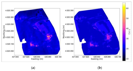
Figure 5.
One of the thermal maps of the Pisciarelli area (a). The same mapping divided in three segments shown by their average temperature (b). The axes correspond to the UTM coordinates; the colour scale is the same for both images.
Temperature differences in areas with vegetation are usually due to different emissivity rather than actual temperature difference [28]. For this reason, the average temperature of the coldest segment was not always the one required as background, as it could include undesired soil features. Hence, it was decided to increase the number of segments every time the average temperature of the cold segment was outside a certain range close to the air temperature. The acceptable range was found from the measurements carried out in Solfatara in Marotta et al., 2019 [13], hereby reprocessed in the histogram in Figure 6, where it is noticeable how the difference between air temperature and BG is almost always ≲5 °C. Such temperature was used as the threshold parameter to understand if the cold segment in the image was the right one: in the presence of a bigger difference, the algorithm repeats the segmentation, increasing the number of required segments and uses the next order one (i.e., the second with four segments, the third with five, etc.). This procedure repeats until the selected segment fits into the 5 °C limit.
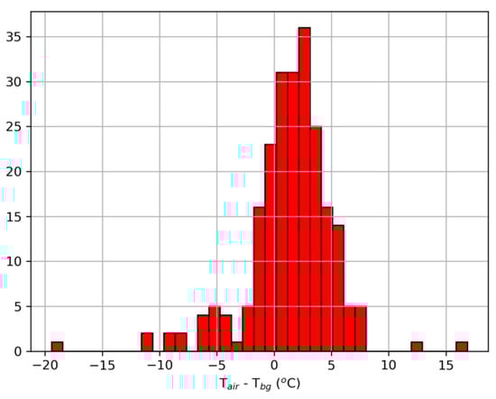
Figure 6.
Histogram showing difference in degrees Celsius between air temperature and BG temperature.
The presence of features not related to anomalous soil within the cold segment could introduce pixels that are the wrong choice to estimate the BG: the statistically less representative pixels were removed in order to estimate the BG. For this reason, it was decided to use the DBSCAN ([16,17] and references therein) algorithm to try to extract the statistically most relevant features.
DBSCAN identifies parts in a given dataset, grouping together the units in the dataset that are within a given “distance” between them. In this case, a simple Euclidean distance in the three-dimensional space made by the pixel position and their temperature was considered. This way, the cold segment was separated into a certain number of clusters from which only the largest ones were selected, covering more than 50% of the segment. The average temperature of the cluster set and its variance were chosen as Tbg of the compound image.
As the flight height of the mappings was not always the same, it is important to take into account how the different distances affect the geometrical blending of the temperatures on the pixels of the hot zones. As the distance between the thermal camera and the subject increases, the ground sampling distance increases, and it also increases the dimensions of the pixels on the ground. This affects the recorded temperature of each pixel as it is the result of the average of all the temperatures that may be contained in the footprint of the pixel: a bigger pixel area results in a net decrease in the recorded temperature with the distance as it contains more and more cold areas. Caputo et al. (2023) [14] gives a rough estimate of this decrease in the amount of about 0.45%/m of distance.
Once the estimated temperature of the background was obtained, and having measured for each flight the relative humidity and the air temperature, it was possible to apply the model of Marotta et al. 2019 [13] to calculate the heat flux and the relative error on each pixel of the compound image. Here, only the pixels with T > Tbg have been selected, as they should be the only ones having a positive flux. However, the majority of these pixels do not have a heat flux meaningfully different from zero. In order to select a set of pixels with a statistically relevant flux, the algorithm selected only those with a heat flux different from zero at more than 3σ (Figure 7). This allowed us to identify and separate the areas with temperature anomalies from the cold background in the image. The estimated temperature decrease [14] with its distance was used to reconstruct the soil temperature from the apparent acquired one by simply rescaling it with altitude. Thus, a rough equalisation of the temperatures read during flights performed at different altitudes was obtained. Afterwards, the flux was recalculated using the equalised temperatures.
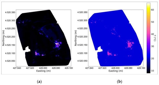
Figure 7.
(a) Mapping of heat flux calculated [13] on all the pixels of the image after the distance correction; (b) pixels with a heat flux different from zero at more than 3σ shown using the average temperature of the cluster. The axes correspond to the UTM coordinates.
The pixels separated from the background were used as the “hot” segment of the thermal composition, and then, the DBSCAN algorithm was again applied to the new hot segment to identify the areas with common features, using the same parameters as the previous clusterisation of the cold one. The result was a set of clusters identified by their average position and size (Figure 8). For each identified cluster, the average temperature, the mean and total heat flux (shown in Figure 9), and other parameters were calculated and stored.
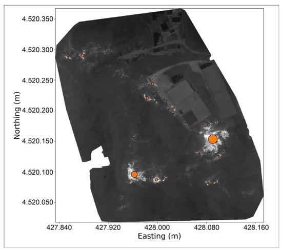
Figure 8.
Example of the outcome of the DBSCAN algorithm on the hot segment: here, each cluster is represented with a simplified representation using the weighted average of the position and temperature of its pixels as the centre of each circle and their average distribution as the radius of each circle which is reported in meters as indicated by the axes in UTM coordinates.
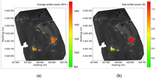
Figure 9.
(a) Average flux (in W/m2) of each identified cluster; (b) total power (in W) of each cluster (37 °C is the average temperature of the hot segment). The axes correspond to the UTM coordinates.
2.2. Temporal Trend of the Heat Flux
The algorithm described allowed us to obtain a set of clusters for each of the analysed flights, each of which is defined by its centre (in UTM coordinates), size, time, date, average temperature, average and total flux, cluster area, and all the relative errors. To understand whether these parameters will show variations over time, it is necessary to figure out if they identify “zones” with coherent characteristics. For this reason, they have been reassembled into one map keeping their temporal information.
Figure 10a shows the distribution of all clusters in the investigated area using one of the background thermal maps as a basis. It is clearly visible how they tend to thicken over the points with thermal anomalies. It was straightforward to apply the DBSCAN algorithm again in order to identify any coherent zone. The parameters of this second iteration were chosen using the average size and temperature distribution of all the clusters and, again, by using a Euclidean distance in the three-dimensional space of position and temperatures.
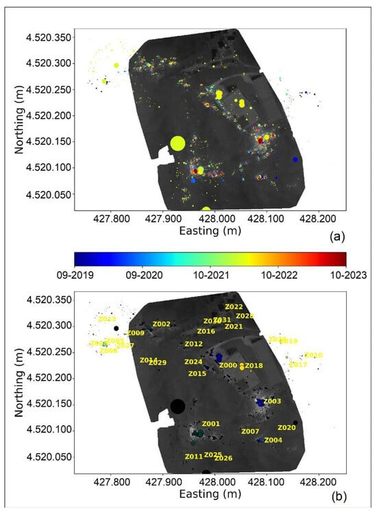
Figure 10.
(a) Temporal representation of the whole cluster set where blue is the oldest and red the most recent. (b) Representation of the zones identified applying the DBSCAN algorithm to the clusters in (a). The mosaic used to represent this image is just one of the created ones: the investigated area is larger on some mosaics, so some points sit outside the silhouette. The radius of the dots is in metres as of Figure 8.
It was possible to identify a great number of zones (Figure 10b), with the most important ones being identified as Z003 and Z001 corresponding, respectively, to PsD1 and PsD2 of Figure 4. For each identified area (Figure 10b), the trend of the heat flux and of the average temperature through time was plotted. It was also necessary to decorrelate the average temperature from the atmospheric one. In order to do so, a Principal Component Analysis (PCA) using a singular value decomposition and keeping all the components was used [29,30,31,32]. The python sklearn package implementation was used [33].
3. Results
The average temperature trend is strongly correlated to the atmospheric temperature for all identified zones and is visible in Figure 11 for Z003 and Z001 which show a very similar pattern in their trend. This kind of correlation (with factors ranging in an interval between 0.85 and 0.99 depending on the zones) was indeed expected mostly because the heat exchange between soil and air is influenced by the external temperature but also because of the effect of pixel blending over distance.
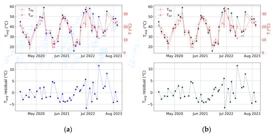
Figure 11.
Temporal trends of the average temperatures of zones Z003 (a) and Z001 (b). On the top row, they are shown together with air and background temperature (both in red). On the bottom row, the residuals of the PCA decorrelation are shown. When not visible, error bars are smaller than the size of the dots.
A Principal Component Analysis [33] was used to decorrelate average soil temperature from air temperatures; the results are shown in the bottom row of Figure 11. The decorrelated temperatures show a very similar trend in each zone where it was possible to calculate it on most of the flights (“main” zones in Figure 12), and it was possible to identify a change in the shape of the trends that seems to span from the summer of 2021 to the summer of 2023.
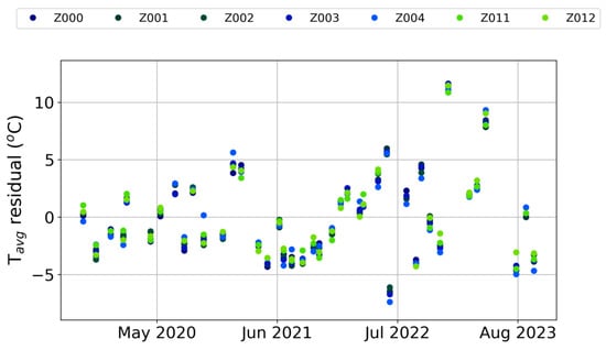
Figure 12.
Trends of the residuals of the PCA decorrelation for the 7 main zones (Z000, Z001, Z002, Z003, Z004, Z011, Z012). When not visible, error bars are smaller than the size of the dots.
Heat flux trends are shown in Figure 13 for zones Z003 and Z001. Z001 shows a correlation factor between the heat flux and the temperature of 0.84 similar to all the other zones (not reported, but, at average, ≳ 0.8), while Z003 is the only one that shows a much lower factor of 0.49. Zone Z003’s heat flux trend shows a modification in its shape from the summer of 2021 to the summer of 2023 like the decorrelated temperatures (see Figure 12).
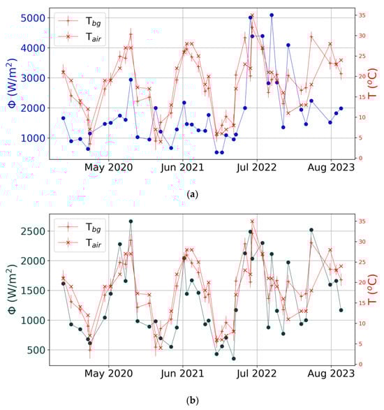
Figure 13.
Temporal trends of the heat flux for zones Z003 (a) and Z001 (b). In red, the air and background temperature are shown. When not visible, error bars are smaller than the size of the dots.
4. Discussion and Conclusions
The observed heat flux trends show a strong correlation with the external temperature for all the identified zones except Z003 which is in contrast to what was observed on the data of La Solfatara in Marotta et al. 2019 [13]. Figure 14 shows how the correlation factor between the flux and Tbg was as low as 0.25. The dependency found between the heat flux and the atmospheric conditions could have different explanations, for example:
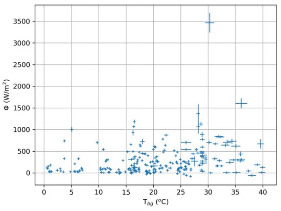
Figure 14.
Heat flux in relation to background temperature for the Solfatara data (reprocessed from Marotta et al., 2019 [13]). Correlation factor is 0.25.
- The superficial behaviour of the aquifer of Pisciarelli is different from the one of the La Solfatara and could disperse heat in a more efficient manner. To try to understand if this is the actual reason behind the strong dependency, it iss necessary to fly over La Solfatara and repeat these types of measurements to see if this effect disappears.
- The temperature measurements taken from the drone averages in the same pixel both the hot areas and the cold areas nearby: this way, the hot areas may be influenced by the outside temperature through this averaging effect. In La Solfatara, this effect was not visible probably because the temperature measurements were carried out at 1 m from the ground, so the entire zone of thermal anomaly was framed in the image. To exclude this possibility, it is necessary to fly over La Solfatara where the areas with comparable agl flight elevation are wider than those at Pisciarelli.
The fact that Z003 does not show the strong correlation seems to confirm the second hypothesis as it had the highest average area of all the other zones during the analysed time period. At the same time, the trends of the decorrelated average temperatures are similar enough to indicate that a similar heat flux dependency on all the zones should be expected. For these reasons, different means to extrapolate heat flux from the surface temperature are being looked into. Remotely sensing the temperature from heights of tens of metres may lead to the possibility that a simpler model, using only the radiative part of the heat flux, may suffice to properly estimate the heat flux, in a similar manner to what is performed in satellite thermal acquisitions [18]. Such a possibility is now being explored to understand which of the previous hypotheses were right and, having finally received the possibility to fly on La Solfatara crater, a set of flight campaigns over La Solfatara to exclude the first possibility are being initiated.
Supplementary Materials
The software DroneFlux used for the analysis of the data is publicly available on Zenodo at https://zenodo.org/record/10551647 (doi: 10.5281/zenodo.10551647) created on 22 January 2024.
Author Contributions
Conceptualization, E.M. and G.A.; methodology and software, R.P. and F.C.; validation, all authors; resources and data curation E.M., R.A., G.A., P.B., A.C. and E.B.S.; writing—original draft preparation, E.M., R.P., E.B.S. and G.A.; writing—review and editing, R.A.P., F.C., T.C. and E.B.S.; supervision, R.P.; project coordination, E.M. All authors have read and agreed to the published version of the manuscript.
Funding
This study was financially supported in the framework of the DPC-INGV B2 Project—WP2 Task 5 (2019–2021).
Data Availability Statement
The full dataset, both input and analysed data, used in this work is publicly available on Zenodo at https://zenodo.org/record/10551266 (doi: 10.5281/zenodo.10551266) created on 22 January 2024.
Acknowledgments
We thank R. Mari from “Città Metropolitana di Napoli—Direzione Strutturazione e Pianificazione dei servizi Pubblici di interesse generale di Ambito Metropolitano—Ufficio S.I.T.—Sistema Informativo Territoriale” for kindly providing ASCII data for the DEM and DSM.
Conflicts of Interest
The authors declare no conflicts of interest.
References
- Friedman, J.D.; Williams, D.L.; Frank, D. Structural and Heat Flow Implications of Infrared Anomalies at Mt. Hood, Oregon, 1972–1977. J. Geophys. Res. 1982, 87, 2793–2803. [Google Scholar] [CrossRef]
- Frank, D.G. Hydrothermal Processes at Mount Rainier, Washington; University of Washington: Seattle, WA, USA, 1985. [Google Scholar]
- Aubert, M. Practical Evaluation of Steady Heat Discharge from Dormant Active Volcanoes: Case Study of Vulcarolo Fissure (Mount Etna, Italy). J. Volcanol. Geotherm. Res. 1999, 92, 413–429. [Google Scholar] [CrossRef]
- Chiodini, G.; Granieri, D.; Avino, R.; Caliro, S.; Costa, A.; Werner, C. Carbon Dioxide Diffuse Degassing and Estimation of Heat Release from Volcanic and Hydrothermal Systems. J. Geophys. Res. Solid Earth 2005, 110, 1–17. [Google Scholar] [CrossRef]
- Hochstein, M.P.; Bromley, C.J. Measurement of Heat Flux from Steaming Ground. Geothermics 2005, 34, 131–158. [Google Scholar] [CrossRef]
- Aubert, M.; Diliberto, S.; Finizola, A.; Chébli, Y. Double Origin of Hydrothermal Convective Flux Variations in the Fossa of Vulcano (Italy). Bull. Volcanol. 2008, 70, 743–751. [Google Scholar] [CrossRef]
- Wang, Y.; Pang, Z.; Hao, Y.; Fan, Y.; Tian, J.; Li, J. A Revised Method for Heat Flux Measurement with Applications to the Fracture-Controlled Kangding Geothermal System in the Eastern Himalayan Syntaxis. Geothermics 2019, 77, 188–203. [Google Scholar] [CrossRef]
- Brombach, T.; Hunziker, J.C.; Chiodini, G.; Cardellini, C.; Marini, L. Soil Diffuse Degassing and Thermal Energy Fluxes from the Southern Lakki Plain, Nisyros (Greece). Geophys. Res. Lett. 2001, 28, 69–72. [Google Scholar] [CrossRef]
- Chiodini, G.; Frondini, F.; Cardellini, C.; Granieri, D.; Marini, L.; Ventura, G. CO2 Degassing and Energy Release at Solfatara Volcano, Campi Flegrei, Italy. J. Geophys. Res. Solid Earth 2001, 106, 16213–16221. [Google Scholar] [CrossRef]
- Isaia, R.; Vitale, S.; Giuseppe, M.G.D.; Iannuzzi, E.; Tramparulo, F.D.A.; Troiano, A. Stratigraphy, Structure, and Volcano-Tectonic Evolution of Solfatara Maar-Diatreme (Campi Flegrei, Italy). GSA Bull. 2015, 127, 1485–1504. [Google Scholar] [CrossRef]
- Isaia, R.; Di Giuseppe, M.G.; Natale, J.; Tramparulo, F.D.; Troiano, A.; Vitale, S. Volcano-Tectonic Setting of the Pisciarelli Fumarole Field, Campi Flegrei Caldera, Southern Italy: Insights Into Fluid Circulation Patterns and Hazard Scenarios. Tectonics 2021, 40, e2020TC006227. [Google Scholar] [CrossRef]
- Sbrana, A.; Marianelli, P.; Pasquini, G. The Phlegrean Fields Volcanological Evolution. J. Maps 2021, 17, 557–570. [Google Scholar] [CrossRef]
- Marotta, E.; Peluso, R.; Avino, R.; Belviso, P.; Caliro, S.; Carandente, A.; Chiodini, G.; Macedonio, G.; Avvisati, G.; Marfè, B. Thermal Energy Release Measurement with Thermal Camera: The Case of La Solfatara Volcano (Italy). Remote Sens. 2019, 11, 167. [Google Scholar] [CrossRef]
- Caputo, T.; Bellucci Sessa, E.; Marotta, E.; Caputo, A.; Belviso, P.; Avvisati, G.; Peluso, R.; Carandente, A. Estimation of the Uncertainties Introduced in Thermal Map Mosaic: A Case of Study with PIX4D Mapper Software. Remote Sens. 2023, 15, 4385. [Google Scholar] [CrossRef]
- Calvari, S.; Spampinato, L.; Lodato, L.; Harris, A.J.L.; Patrick, M.R.; Dehn, J.; Burton, M.R.; Andronico, D. Chronology and Complex Volcanic Processes during the 2002–2003 Flank Eruption at Stromboli Volcano (Italy) Reconstructed from Direct Observations and Surveys with a Handheld Thermal Camera. J. Geophys. Res. 2005, 110, 2004JB003129. [Google Scholar] [CrossRef]
- Cirillo, F.; Avvisati, G.; Belviso, P.; Marotta, E.; Peluso, R.; Pescione, R.A. Clustering of Handheld Thermal Camera Images in Volcanic Areas and Temperature Statistics. Remote Sens. 2022, 14, 3789. [Google Scholar] [CrossRef]
- Cirillo, F.; Avvisati, G.; Belviso, P.; Marotta, E.; Peluso, R.; Pescione, R. STARTED (StaTistical Analysis clusteRed ThErmal Data). Software. Available online: https://zenodo.org/records/5886707#.YuXahBxBzIU (accessed on 21 January 2022).
- Silvestri, M.; Marotta, E.; Buongiorno, M.F.; Avvisati, G.; Belviso, P.; Bellucci Sessa, E.; Caputo, T.; Longo, V.; De Leo, V.; Teggi, S. Monitoring of Surface Temperature on Parco Delle Biancane (Italian Geothermal Area) Using Optical Satellite Data, UAV and Field Campaigns. Remote Sens. 2020, 12, 2018. [Google Scholar] [CrossRef]
- Vilardo, G.; Ventura, G.; Bellucci Sessa, E.; Terranova, C. Morphometry of the Campi Flegrei Caldera (Southern Italy). J. Maps 2013, 9, 635–640. [Google Scholar] [CrossRef]
- PIX4Dmapper: Professional Photogrammetry Software for Drone Mapping. Available online: https://www.pix4d.com/product/pix4dmapper-photogrammetry-software (accessed on 27 October 2022).
- Analist Group. Available online: https://www.analistgroup.com/ (accessed on 18 January 2024).
- Flynn, L.P.; Mouginis-Mark, P.J.; Gradie, J.C.; Lucey, P.G. Radiative Temperature Measurements at Kupaianaha Lava Lake, Kilauea Volcano, Hawaii. J. Geophys. Res. 1993, 98, 6461–6476. [Google Scholar] [CrossRef]
- Pinkerton, H.; James, M.; Jones, A. Surface Temperature Measurements of Active Lava Flows on Kilauea Volcano, Hawai′ i. J. Volcanol. Geotherm. Res. 2002, 113, 159–176. [Google Scholar] [CrossRef]
- Spampinato, L.; Calvari, S.; Oppenheimer, C.; Boschi, E. Volcano Surveillance Using Infrared Cameras. Earth Sci. Rev. 2011, 106, 63–91. [Google Scholar] [CrossRef]
- Ball, M.; Pinkerton, H. Factors Affecting the Accuracy of Thermal Imaging Cameras in Volcanology. J. Geophys. Res. 2006, 111, 2005JB003829. [Google Scholar] [CrossRef]
- Dehn, J.; Dean, K.; Engle, K.; Izbekov, P. Thermal Precursors in Satellite Images of the 1999 Eruption of Shishaldin Volcano. Bull. Volcanol. 2002, 64, 525–534. [Google Scholar] [CrossRef]
- ESRI. ArcGIS Desktop: Release 10; Environmental Systems Research Institute, Inc.: Redlands, CA, USA, 2011. [Google Scholar]
- Clausing, L.T. Emissivity: Understanding the Difference between Apparent and Actual Infrared Temperatures. Fluke Application Note, Fluke Education Partnership Program. Available online: www.fluke.com (accessed on 18 January 2024).
- Minka, T. Automatic Choice of Dimensionality for PCA. In Advances in Neural Information Processing Systems; MIT Press: Cambridge, MA, USA, 2000; Volume 13. [Google Scholar]
- Tipping, M.E.; Bishop, C.M. Probabilistic Principal Component Analysis. J. R. Stat. Soc. Ser. B Stat. Methodol. 1999, 61, 611–622. [Google Scholar] [CrossRef]
- Halko, N.; Martinsson, P.G.; Tropp, J.A. Finding Structure with Randomness: Probabilistic Algorithms for Constructing Approximate Matrix Decompositions. SIAM Rev. 2011, 53, 217–288. [Google Scholar] [CrossRef]
- Martinsson, P.-G.; Rokhlin, V.; Tygert, M. A Randomized Algorithm for the Decomposition of Matrices. Appl. Comput. Harmon. Anal. 2011, 30, 47–68. [Google Scholar] [CrossRef]
- Taskesen, E. Pca: Pca Is a Python Package That Performs the Principal Component Analysis and to Make Insightful Plots. Available online: https://erdogant.github.io/pca/pages/html/index.html (accessed on 27 October 2022).
Disclaimer/Publisher’s Note: The statements, opinions and data contained in all publications are solely those of the individual author(s) and contributor(s) and not of MDPI and/or the editor(s). MDPI and/or the editor(s) disclaim responsibility for any injury to people or property resulting from any ideas, methods, instructions or products referred to in the content. |
© 2024 by the authors. Licensee MDPI, Basel, Switzerland. This article is an open access article distributed under the terms and conditions of the Creative Commons Attribution (CC BY) license (https://creativecommons.org/licenses/by/4.0/).