Combining Multi-View UAV Photogrammetry, Thermal Imaging, and Computer Vision Can Derive Cost-Effective Ecological Indicators for Habitat Assessment

Abstract

Recent developments in Unmanned Aircraft Vehicles (UAVs), thermal imaging, and Auto-machine learning (AutoML) have shown high potential for precise wildlife surveys but have rarely been studied for habitat assessment. Here, we propose a framework that leverages these advanced techniques to achieve cost-effective habitat quality assessment from the perspective of actual wildlife community usage. The framework exploits vision intelligence hidden in the UAV thermal images and AutoML methods to achieve cost-effective wildlife distribution mapping, and then derives wildlife use indicators to imply habitat quality variance. We conducted UAV-based thermal wildlife surveys at three wetlands in the Rainwater Basin, Nebraska. Experiments were set to examine the optimal protocols, including various flight designs (61 and 122 m), feature types, and AutoML. The results showed that UAV images collected at 61 m with a spatial resolution of 7.5 cm, combined with Faster R-CNN, returned the optimal wildlife mapping (more than 90% accuracy). Results also indicated that the vision intelligence exploited can effectively transfer the redundant AutoML adaptation cycles into a fully automatic process (with around 33 times efficiency improvement for data labeling), facilitating cost-effective AutoML adaptation. Eventually, the derived ecological indicators can explain the wildlife use status well, reflecting potential within- and between-habitat quality variance.

1. Introduction

Quantifying variance in habitat quality (the ability of the environment to provide conditions appropriate for individual and population persistence) within and between wetlands is essential to direct wildlife conservation efforts [1,2,3,4]. Wildlife/habitat use (how wildlife utilize the physical and biological resources in a habitat) can be a critical indicator to reflect potential habitat quality variance. Ecological managers typically estimate wildlife abundance to understand habitat status for quality assessment [5,6,7]. The major challenge encountered is the difficulty in accurately and precisely localizing wildlife individuals and the actual habitat areas occupied by wildlife [1,2,8,9]. These data are essential for further analyses of wildlife distribution and habitat usage.

Traditional wildlife survey techniques (e.g., by visual identification from ground observation or piloted aircraft) are often limited by the species’ sensitivity and covert habitat environment or the coarse spatial resolution of aerial imagery, making accurate wildlife censusing infeasible [6,10,11]. This is especially true for small and sensitive wildlife (e.g., shorebirds and waterfowl) usually living in remote areas with dense vegetation cover [10]. To enhance accuracy, novel technologies, such as camera traps, acoustic recorders, and animal-borne telemetry, have been widely used in wildlife surveys [12,13]. However, collecting remote sensing imagery by aerial surveys is still considered one of the most efficient observation approaches [5,10,11], as it creates permanent visual records, which enable repeatable inspections and precise wildlife localization [6,14,15].

Meanwhile, advances in Unmanned Aircraft Vehicle (UAV) platforms, intelligent computer vision, and photogrammetry sensors have greatly enhanced the accuracy and efficiency of wildlife surveys [16,17]. Small UAVs are cost-effective for acquiring high-resolution wildlife imagery, as they provide dense temporal coverage and flexible payload arrangements with minimal wildlife disturbances [11,18,19]. UAVs offer images with spatial resolution that are clear enough to observe individual wildlife and thus have been used for diverse ecological applications, such as wildlife population censusing [5,6,20,21], nest detection [22,23], and poaching activity tracking [24]. Successful application has been noticed in a broad range of species, from big animals like whales, elephants, deer, elk, seals, and crocodiles [6,25,26,27,28], to small animals like rabbits, shorebirds, and koalas [10,23,29,30,31,32]. However, detection errors in RGB images (e.g., missed counting or misidentification) are very likely to occur when dense vegetation is present [14]. Thermal–infrared sensors, taking advantage of the apparent gradient contrast between wildlife and the background [14], were found to be useful in detecting elusive species in habitats with complex environments [16], as thermal images can effectively decrease the counting errors that occur in RGB imagery [6,32,33] or based on purely human vision [34].

Traditional wildlife detection is labor-intensive and time-consuming when conducted by manual counting [5,6]. AutoML has shown encouraging machine intelligence in automated wildlife detection [10,21]. Studies have found that UAV-image-based wildlife censusing is much more accurate and precise than human counting (using binoculars). Basic computer vision approaches are sufficient to detect wildlife in environments without complex land covers, such as thresholding based on the spatial–spectral patterns of the targets [16]. Seymour et al. [6] used thresholding approaches to detect seals based on morphological patterns (e.g., temperature, size, and shape) by UAV thermal images. Rey et al. [21] detected large mammals in a savannah environment based on a histogram of colors in UAV RGB images. Hodgson et al. [5] used a Support Vector Machine to census bird decoys in a simulated wetland colony based on UAV RGB images.

However, these AutoMLs require full or partial human intelligence to determine the features or threshold used for wildlife detection. These low-level features carry limited semantic meanings, which constrains their ability to describe wildlife targets and makes them unscalable to complex environments. Novel AutoML, such as Convolutional Neural Networks (CNNs), which construct spatial–spectral features in an end-to-end manner, have shown potential to fulfill the demands of wildlife detection in more complex environmental settings [16,24,35]. Kellenberger et al. [36] developed an active-learning CNN framework for large mammal censusing. Hamilton et al. [30] utilized Faster R-CNN and YOLO (You Only Look Once) combined with thermal imagery to detect koalas (with a size of 60–85 cm) in complex forest areas. Kellenberger et al. [37] developed a lightweight CNN architecture to detect seabirds (with a size of 37–48 cm and 90–145 cm wingspan) using UAV RGB imagery. Chen et al. [32] combined thermal imagery, RGB imagery, and YOLO to detect cranes (with sizes of 90 to 102 cm and 180–240 cm wingspan) during nighttime.

Although UAV, thermal, and AutoML show high potential for cost-effective wildlife surveys, no studies explicitly examined their effectiveness for shorebirds or waterfowl in wetland habitats, given their small sizes (with sizes of 37–56 cm) and high sensitivity. Little is known about how to take advantage of the intelligence merits of these advanced technologies for practical habitat use/assessment [16]. Moreover, attention so far has been mainly paid to developing complex algorithms for better wildlife detection accuracy. AutoML that require tedious preprocessing procedures and startup time may not be feasible, even if they can return high performance [10]. No study has systematically addressed the labor, expertise, and computing investment (including data collection and labeling, model training, and deployment) from practical perspectives to achieve cost-effective wildlife surveys and habitat quality assessment.

To bridge the gap between theory and practice in habitat assessment, we proposed a cost-effective framework for assessing wetland habitats from the perspective of wildlife communities. The framework utilizes machine intelligence to model the relationship between UAV thermal images and wildlife objects, and to segment water land cover so that wildlife and their corresponding occupied area in thermal images can be automatically located and mapped. These mapping products are then transformed into wildlife use proxies to infer habitat quality variation. The labor, expertise, and computing investment involved are systematically handled from the perspective of cost-effective and implementable wetland assessment. The framework is composed of three main stages:

(1)

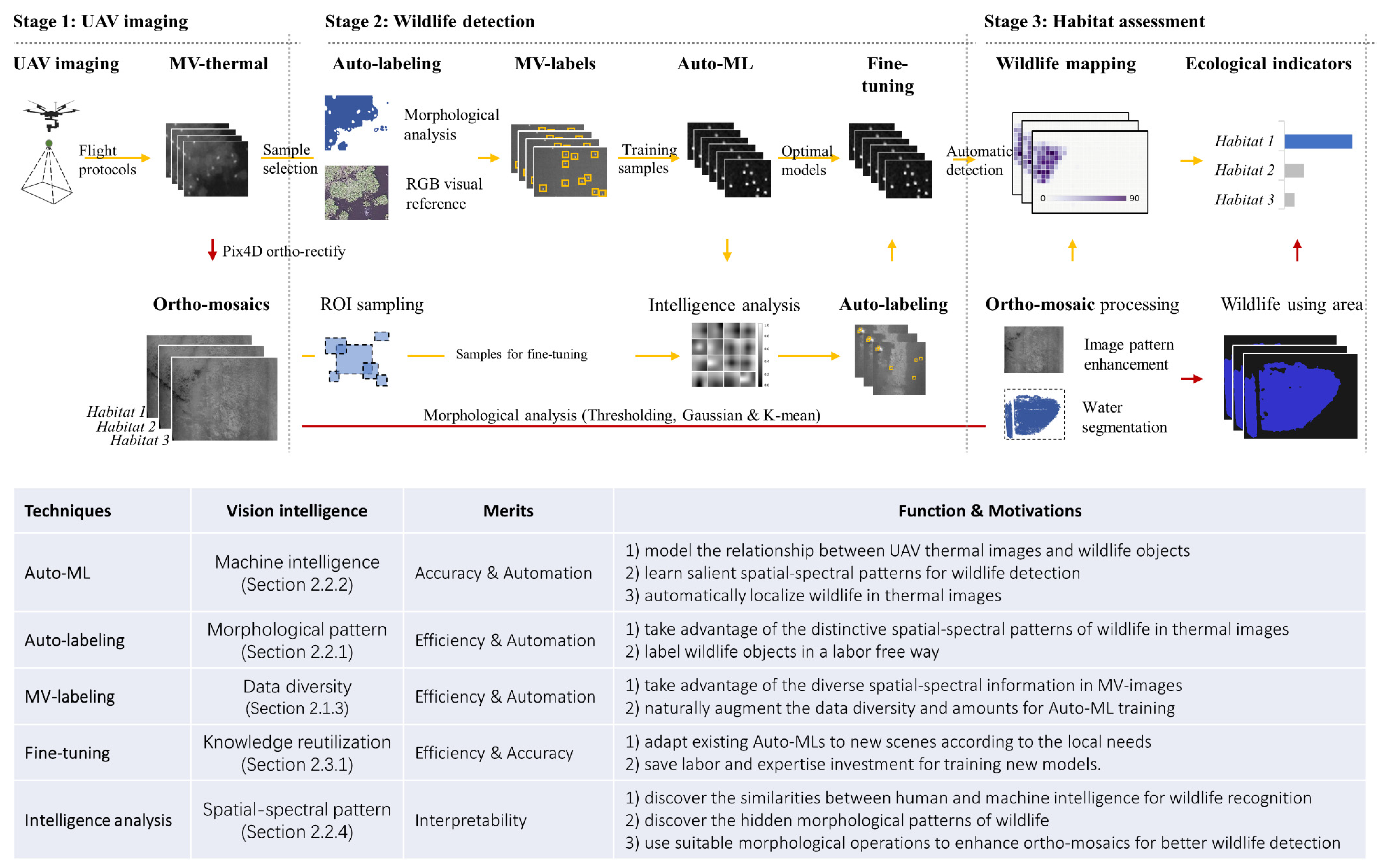
The UAV imaging stage was designed to explore the potential of UAV photogrammetry for high-quality wildlife data collection. UAVs and thermal imaging were used and tested at different flight heights to conduct wildlife surveys in wetland habitats, and thermal ortho-mosaics were produced to detect wildlife (Section 2.1).

(2)

The wildlife detection stage was designed to explore the potential of thermal images, multi-view (MV) UAV image structure, and AutoML to achieve labor-free wildlife and inundation (water area) mapping (Section 2.2). Experiments with various AutoML architectures, training data sizes, and feature types were conducted to discover the optimal configuration of human labor, expertise, and computing investment for wildlife distribution mapping.

(3)

The habitat assessment stage was designed to explore how to transform the wildlife counts and distribution information into ecological indicators (including wildlife counts, usage area, and usage efficiency for intra- and inter-habitat comparison) to reflect the level of wildlife capacity and wildlife use (Section 2.3).

As depicted in Figure 1, rather than purely developing sophisticated methods for wildlife detection, we focus on maximizing vision intelligence during habitat assessment (by replacing any human involvement where possible) and on how to transform detection or mapping results into meaningful information to assist habitat assessment processes. We define intelligence as the potential knowledge derived from data, technologies, and models that can be used to improve automation, efficiency, and accuracy for wetland habitat assessment. Specifically, by exploiting the vision intelligence of thermal, UAV imaging and AutoML, we transform the traditional labor-intensive and expertise-dependent habitat assessment framework into labor-free but robust wildlife and habitat mapping processes. The major cost savings of this framework, compared with traditional AutoML adaptation workflow, come from the three intelligent techniques: auto-labeling, MV labeling, and fine-tuning.

2. Materials and Methods

2.1. UAV Imaging

2.1.1. Study Area

The survey areas included publicly managed playa wetlands in the Rainwater Basin, Nebraska, United States. These playas provide critical migration stopover habitats (habitats with physical or biological features essential to the conservation of particular species) for millions of migratory birds in the Central Flyway, which helps to meet the bioenergetic needs of the wildlife during spring migration [38]. Intensive farming activities have caused significant modifications to the local natural landscapes, which have caused deterioration in the ecological functionality of the wetlands and reduced the bioenergetic capacity for spring migrating birds [39,40].

Three wetlands were chosen to collect aerial wildlife imagery from, including Straightwater wildlife management area (WMA), Smith waterfowl production area (WPA), and Johnson WMA (Figure 2). These habitats were selected in a manner of even distribution (from west to east) in the Rainwater basin, encompass different seasons and weather temperatures, and are far from the populated area to ensure less impact from human activity on wildlife preference. The common wildlife species appearing during spring migration on these wetlands include greater white-fronted geese (Anser albifrons), mallards (Anas platyrhynchos), northern pintails (Anas acuta), and lesser snow geese (Chen caerulescens) [38], while the actual wildlife encountered in this study are mostly mallards (with an actual size of 37–56 cm estimated by human observation over UAV images).

2.1.2. UAV Flight Protocols

The Matrice 600 pro (DJI, Shenzhen, Guangdong, China), a hexacopter rotary-wing UAV, was used to conduct the aerial survey, loaded with the FLIR Duo Pro R (FLIR, Wilsonville, OR, USA). The sensor has a radiometric thermal lens (512 × 640 px) with a spectral range of 7.5–13.5 μm and an optical lens (3000 × 4000 px) onboard, capturing thermal and RGB images at the same time-spatial sequences. All flights were conducted at each wetland in 2018–2019 at two flight heights: 61 m (200 feet) and 122 m (400 feet) above ground level (AGL) to test the optimal flight height for wildlife imaging. Every flight mission was designed with 80% frontal overlap and 70% side overlap with the nadir setting, covering an area of approximately 0.11 km² (30 acres) within 15 min (Supplementary Material S1).

2.1.3. MV UAV Images to Ortho-Mosaics

The UAV images are also called MV images [41,42,43], which create diverse spatial–spectral patterns as they are collected from adjacent overlapped flight paths with different positions and angles (Supplementary Material S2). An ortho-mosaic of each site was produced in Pix4D (Pix4D, Prilly, Switzerland), where every MV image was ortho-rectified. The value of each pixel in the ortho-mosaic is a weighted mean of the corresponding pixels from the MV images.

Eventually, three MV UAV datasets with large groups of wildlife presented were successfully collected (one dataset from each site) to produce three thermal ortho-mosaics. The MV image dataset in Straightwater WMA was chosen to collect data to train and validate AutoML and select the optimal model, as this wetland has the most distinctive wetland features (water, land, and wildlife), making it easy to realize visual wildlife verification and geographic modeling (Figure 2). The ortho-mosaics of each wetland habitat were used to test the AutoML for wildlife detection and distribution mapping. Details of these datasets are documented in Figure 3d.

2.2. Wildlife Detection

2.2.1. AutoMV Labeling

The primary costs of using AutoML in practical applications are the labor and expertise costs of data organization (data collection and labeling). The AutoMV labeling process, designed to simulate human visual perception, achieves intelligent data organization by segmenting wildlife objects in MV thermal images from their background using a series of human-determined morphological operations and thresholds (including pixel intensity, area, and solidity, as depicted in Figure 3a):

(1)

Segment the image regions with pixel values larger than a local adaptive threshold, calculated as the local mean plus two times the local variance within a 16 × 16 sliding window for each pixel;

(2)

Remove image regions with area and solidity below thresholds determined by local knowledge of the wildlife shape and size;

(3)

Select the images with high-level labeling quality as training samples, in visual reference to the RGB images. The high-quality labels are determined as images with more than 50% wildlife. Wildlife are accurately labeled without obvious false positive labels (objects that are incorrectly labeled as birds).

From the Straightwater WMA dataset, we collected 128 MV images containing 698 wildlife objects (many of which are the same wildlife individuals labeled in different MV images) as training samples. Other images were further labeled as validation samples by a thorough human inspection, including 226 images (containing 8356 wildlife objects). The same auto-labeling process was applied to each orthomosaic and was labeled as test data. Related datasets were archived online (Supplementary Material S6).

2.2.2. Experiments with Different AutoML

The level of machine or human intelligence determines how AutoML processes input images to construct salient features for detection tasks (Figure 3b). We selected 8 AutoMLs with 3 AutoML types, grouped as thresholding, decision tree (ACF, Harr, HOG, and LBP feature), and CNN architectures (Faster R-CNN, SSD, and YOLO4), to represent different levels of machine/human intelligence involved in wildlife detection. These AutoML were selected because of reports of their reliability and efficiency in small object detection using spatial–spectral features [40,44,45]. The spatial–spectral nature of the features also makes them easy to identify wildlife morphological patterns for later machine intelligence analyses. Detection architecture demanding complex design and redundant tuning was intentionally avoided to ensure cost-effective generalization.

From thresholding to decision trees to CNNs, the level of machine intelligence increases while human intelligence decreases. The thresholding architecture (the same as the AutoMV labeling technique) represents the most typical image threshold architecture, requiring users to determine the specific features and segmentation thresholds for object detection (human intelligence dominated) [6]. Decision trees were tested with 4 different spatial–spectral patterns (including Haar-like ACF, HOG, and LBP features), representing typical machine learning architectures [46,47,48,49]. Different feature types indicate different spatial–spectral patterns used to describe wildlife objects. Haar, HOG, and LBP focus on local intensity change (e.g., edge and line features), gradient variance, and texture, respectively, and ACF is the aggregation of the three feature patterns. Decision trees require users to pre-determine the feature types, while AutoML automatically selects the most salient local patterns for local tasks (semi-machine intelligence). CNNs, including Faster R-CNN [50], SSD (Single Shot Detector), and YOLO [30] represent novel state-of-the-art deep learning architectures that learn and select optimal spatial–spectral features for local tasks in fully end-to-end manners (fully machine intelligence). All of the methods were developed in Matlab 2023b, with a GeForce RTX 3060 GPU.

2.2.3. Experiments for Optimal Model Selection

The number of training samples denotes different levels of labor, expertise, and computing investments. To achieve cost-effective wildlife mapping, we grouped the training datasets into 5 groups containing 8, 16, 32, 64, and 128 training images (all training samples were randomly selected) to study the effects of training sample sizes on detection performance. Data augmentation techniques like random image rotation, reflection, and contrast were applied to further augment the data diversity. Every AutoML was trained 5 times over each training dataset and then applied to the validation dataset to check performance. The mean F1 score (Supplementary Material S5) of each AutoML (over 5 times training) at each training sample size was calculated. The model with a relatively less training sample size but higher detection performance (F1 score) was selected as the optimal AutoML model for final wildlife detection. F1 scores take both precision (indication of how many detections are correctly predicted as wildlife) and recall (indication of how many real wildlife are correctly detected) into account. A high F1 value indicates both high precision and recall, and vice versa.

2.2.4. Intelligence Analyses

Analyses of the intelligent components in the well-trained AutoML were conducted to enhance the understanding of wildlife morphological patterns and discover the similarities between machine and human intelligence. Filter analyses reflect which morphological patterns were commonly suitable for describing wildlife objects. We selected three AutoML (including the thresholding, optimal decision tree, and optimal CNN architectures) and compared the optimal feature filters used or learned by these AutoML. Feature analyses reflect which and how spatial–spectral features were constructed by full machine intelligence (by the optimal CNN). We selected three image samples representing different environmental settings (land cover compositions) and extracted the salient CNN features learned from each CNN layer to show the feature construction process. Then, the t-SNE clustering technique was employed to analyze the spatial–spectral separability of these salient features over different land covers (including water, vegetation, and wildlife). The t-SNE is a technique for squeezing high-dimensional features into low-dimensional feature space without disturbing the feature distribution [51].

2.3. Application for Habitat Assessment

2.3.1. Wildlife Distribution by Fine-Tuning

Models trained on samples from the Straightwater WMA may not generalize well to data patterns in other sites. Training a model that perfectly fits local data from scratch is expensive in terms of labor and time. Therefore, this study employed a fine-tuning technique to leverage the performance of a pre-trained model, minimizing additional labor, time, and computing costs.

Fine-tuning refers to using pre-trained models (Detector-SW) that have already learned something beforehand and training that model further with the same or different datasets. From the ortho-mosaic of each habitat, we selected 2–4 regions of interest (ROIs) that contained enough high-quality wildlife objects (according to the intelligence analyses; detailed dataset for the fine-tuning process is displayed in Supplementary Material S4). We then labeled the wildlife objects inside with the AutoMV labeling technique (described in Section 2.2.1), but first used the optimal AutoML to detect the areas most likely to contain wildlife objects. From these ROIs, we derived and augmented around 128 wildlife samples (according to the optimal training sample sizes) for each wetland and used these new data to fine-tune the base model (denoted as Fine tuning-SW, Fine tuning-SM, and Fine tuning-JS). Data augmentation techniques, such as random image rotation, reflection, contrast adjustment, and Gaussian smoothing kernel filtering, were applied to the original training samples to increase the diversity of the training dataset and prevent the algorithms from overfitting. All parameters in the pre-trained model were set as trainable during fine-tuning.

These fine-tuned models were then applied to their corresponding ortho-mosaics for wildlife detection. The precision–recall (PR) curve for each test was recorded for comparison. The PR curve illustrates the relation between precision and recall at different confidence scores, where increases in either recall or precision will increase the area under the curve line.

Once wildlife objects are successfully detected, wildlife abundance can be easily acquired for each wetland habitat. Kernel density was then applied to the wildlife locations to map the wildlife distribution.

2.3.2. Wildlife Using Area by Morphological Analysis

Wildlife density (dividing the wildlife abundance by the habitat area) reflects the level of wetland usage by wildlife, which is convenient for intra-habitat comparison. However, wildlife density may be biased by incomplete recognition of habitats if wildlife communities in wetlands are not fully covered in the dataset (due to the limitation of UAV flight duration). To account for this bias, we developed two wildlife usage areas: the actual usage area and the theoretical usage area.

Actual wildlife usage areas indicate the area occupied by wildlife, which is derived by mapping habitats using a 10 × 10 m fishnet grid and counting the amount of wildlife individuals in each 10 × 10 m block. The blocks in which at least one individual wildlife object exists were regarded as effective wildlife using blocks (with each block indicating an area of 100 ${\mathrm{m}}^2$). Theoretical wildlife usage areas indicate the areas in wetlands theoretically suitable for wildlife use based on expert knowledge, which is derived by thresholding the inundated wetland areas from the thermal ortho-mosaics by observing the temperature of water content and a series of morphological analyses (Supplementary Material S3).

2.3.3. Ecological Indicators for Habitat Assessment

Given the total number of detected wildlife in the wetland ($N$) and the area used by wildlife, comprehensive density-based wildlife and habitat use indicators, such as habitat use efficiency, can be calculated to quantify how many wildlife objects are in each $m^2$:

$$Wildlife use efficiency=\frac{N}{Wildlife usage area},$$

(1)

$$Habitat use efficiency=\frac{Actual wildlife usage areas}{Theoretical wildlife usage areas}.$$

(2)

Wildlife use efficiency, calculated as the ratio of wildlife abundance to actual or theoretical wildlife usage area, focuses on different aspects of habitat quality. Therefore, it can be used as an indicator to infer habitat quality variance among different habitats. Wildlife use efficiency reflects the potential wildlife capacity of the habitat, while actual and theoretical wildlife usage area reflects the general wildlife capacity of the whole habitat. Habitat use efficiency reflects the level of wetland use by wildlife. All of these proxies are derived from the perspective of the wildlife community and are normalized by wildlife using areas to counteract the bias from habitats with different sizes. This makes them ideal for cross-habitat comparisons. Local ecological managers can use these indicators to develop proactive conservation practices for precision conservation.

3. Results

3.1. Experiment for Wildlife Detection

The UAV flights created 15 cm ground sample distance (GSD) at 122 m AGL (Figure 4a) and 7.5 cm GSD at 61 m AGL in the thermal imagery. Individual wildlife produced at least four pixels around 18–22 °C at 121 m AGL and at least sixteen pixels around 24–29 °C at 61 m AGL. The results showed that, compared with RGB imagery, UAV thermal imagery enabled fast and convenient identification of wildlife by human vision, even when dense environmental noise like vegetation was presented. Compared with 122 m AGL, flights conducted at 61 m AGL provided better spatial resolution and stronger thermal signals for wildlife. Furthermore, field observation showed that 61 m AGL altitude created minor disturbances to the wildlife. Therefore, experiments and results in the detection stages were based on the datasets captured at 61 m AGL.

Examples of the detection results show that AutoML can properly detect most of the wildlife in images (Figure 4b). The F1 score for thresholding was used as the benchmark performance for comparison (F1 value, 72.0%, Figure 4c), reflecting the basic effectiveness of human intelligence in wildlife pattern recognition. For decision tree architectures, the Harr feature returned the optimal F1 performance of 53.2–84.8%, which is better than HOG, ACF, and LBP features. This indicates the importance of edge and line features for describing morphological patterns of wildlife in thermal imagery. The Faster R-CNN returned the best detection performance (F1 value, 72.7–93.9%), outperforming all other CNNs and AutoML, as well as the optimal decision tree ($p=0.012$) and thresholding architecture ($p=0.00002$) at all training sample sizes. The superior performance of CNN features indicates the effectiveness of CNNs in extracting salient spatial–spectral features for wildlife detection. The performance of Faster R-CNN reaches a relatively stable status with around 120 training samples, indicating a cost-effective AutoML configuration. Positive relations between detection performance and training sample size can be found for most AutoML, while obvious overfitting issues occur with HOG- and LBP-based decision tree architectures. Recently developed AutoML, such as YOLO and SSD, returned lower performance than Faster R-CNN, probably due to the following: (1) they have high architecture complexity, which required more data diversity and amounts to fulfill a complete learning process; (2) they use multi-scale design when they use a multi-scale feature extraction backbone to condense image information, resulting in loss of information for small objects in this study [1,2]. The incomplete training processes for SSD and YOLO show that more training data are required.

The optimal Faster R-CNN detector (with 120 wildlife samples) was used as the base model (Detector-SW) and applied at each wetland. In general, encouraging detection results (Figure 4d) were received at Straightwater WMA (AP $\approx$ 0.957) and Smith WPA (AP $\approx$ 0.923), but relatively lower detection results were received at Johnson WPA (AP $\approx$ 0.820). The fine-tuning process improved detection performance by 4.4% at Smith WPA and 10.3% at Johnson WPA. No obvious differences were observed at Straightwater WMA, indicating that the MV training data can fulfill a complete learning process for the Faster R-CNN architecture.

3.2. Experiment for Intelligence Analyses

As the performance analyses above show, the choice of feature types used to describe the morphological patterns of the wildlife objects (appearance and shape) is important for successful wildlife detection from thermal images. The filter analyses further reveal that humans and machines are consistent in using superficial appearance and shape patterns, especially line and edge patterns, for wildlife recognition.

However, the performance of these morphological patterns is constrained by the limited recognition of human intelligence, which identifies objects based on superficial appearance and shape. Traditional computer vision techniques (such as thresholding and decision trees) utilize hand-engineered features for detection tasks. These features are usually primitive and carry superficial semantic intention, making them unscalable to complex environment settings. Without the guidance of human knowledge, the CNN architecture looks for specific features (like dots, corners, and edges) well-suited to describe wildlife (Figure 5a). This allows CNNs to properly separate wildlife clusters from other land cover clusters (Figure 5b).

3.3. Experiment for Habitat Assessment

Eventually, we applied the Detector-SW, Fine tuning-SM, and Fine tuning-JS on Straightwater WMA, Smith WPA, and Johnson WPA for final wildlife detection. There were 429, 2735, and 328 wildlife objects, respectively, detected from the three wetlands (distributed in 12,000, 10,300, and 10,400 ${\mathrm{m}}^2$ of actual usage area). The actual wildlife use efficiency for each habitat was calculated as 3.6, 28.6, and 3.2 wildlife per 100 ${\mathrm{m}}^2$ (Figure 6), respectively, indicating that Smith WPA may contain higher quality habitat than the other wetlands sampled.

The morphological analysis shows that the suitable areas for wildlife use for Straightwater WMA, Smith WPA, and Johnson WPA are 311,335, 555,693, and 298,084 ${\mathrm{m}}^2$, respectively. This results in theoretical wildlife use efficiency of 0.14, 0.53, and 0.11 wildlife per 100 ${\mathrm{m}}^2$ for the respective habitats. The high level of wildlife counts and wildlife use efficiency imply that Smith WPA may have a better wildlife capacity and quality. The percentages of suitable wetland areas (for wildlife) developed by wildlife for each habitat are 3.8%, 1.8%, and 3.5%, respectively. This indicates relatively high-level wetland exploitation for Straightwater WMA and Johnson WPA, in comparison to Smith WPA.

4. Discussion

As shown in the above results, the framework integrating UAVs, thermal imaging, and CNNs showed great potential to achieve cost-effective habitat assessment surveys. In this section, we will focus on addressing key usage and the potential of this framework for future success.

4.1. High-Quality Wildlife Surveys

The balance between flight heights and wildlife disturbance is essential for successful UAV wildlife surveys. Consistent with many previous studies [6,30], the study shows that thermal imagery can effectively detect birds in cryptic environments (e.g., Smith WPA). The distinct thermal signature simplifies wildlife detection for both human and computer vision. However, the relatively coarse spatial resolution of thermal sensors and the high sensitivity of bird species to UAV presence may limit data quality. Close-up imaging operations can increase spatial image resolutions but may produce massive wildlife disturbance [52]. Thus, an optimal flight height (61 m in this case) must be carefully chosen, based on the sensors, UAV models, size of wildlife species, and habitat status, to avoid significant wildlife disturbances and obtain meaningful outputs.

4.2. Vision Intelligence for Cost-Effective Habitat Quality Assessment

Vision intelligence aspects from thermal images, MV image structure, and AutoML fine-tuning can facilitate cost-effective automated wildlife detection when properly leveraged. The 72% F1 score achieved by the thresholding detector provides a benchmark for the auto-labeling process, given their shared working procedure (Figure 3c). Thermal imagery is unique in its anomaly effect on geographic elements with high temperatures, making it easy to identify warm-blooded wildlife. Human intelligence, mainly visual knowledge of wildlife morphology in thermal images, can be transferred to machine intelligence by automatic computer programs (auto-labeling techniques). The auto-labeling technique simulates human vision logic, using morphological rules for wildlife identification, resulting in labor-free data-labeling processes. MV images resulting from the unique UAV photogrammetry process contain rich data diversity freely available for AutoML training. Advanced AutoML, such as CNN, are usually ravenous for data amounts and data diversity [53]. Thus, leveraging this diversity by MV labeling helps to create high-quality training datasets, facilitating cost-effective AutoML learning and tuning cycles. AutoML fine-tuning techniques are unique in the way that they reuse machine vision knowledge in a pre-trained AutoML and adapt it to new cases [16]. Leveraging the intelligent merits of each technique enables a cost-effective mapping framework (within minutes) for wetland wildlife survey, in which the framework can be quickly deployed in various environments and real applications without tremendous labor, expertise, or computing investments. As depicted in

Table 1. Labor, expertise, or computing investment analyses.

	Labeling (Seconds)		Training (Minutes)
Investments	$\mathrm{M}\mathrm{a}\mathrm{n}\mathrm{u}\mathrm{a}\mathrm{l}\mathrm{L}\mathrm{a}\mathrm{b}\mathrm{e}\mathrm{l}\mathrm{i}\mathrm{n}{\mathrm{g} }^1$	$\mathrm{A}\mathrm{u}\mathrm{t}\mathrm{o}-\mathrm{L}\mathrm{a}\mathrm{b}\mathrm{e}\mathrm{l}\mathrm{i}\mathrm{n}{\mathrm{g} }^2$	$\mathrm{T}\mathrm{r}\mathrm{a}\mathrm{i}\mathrm{n}\mathrm{i}\mathrm{n}{\mathrm{g} }^3$	$\mathrm{F}\mathrm{i}\mathrm{n}\mathrm{e}-\mathrm{T}\mathrm{u}\mathrm{n}\mathrm{i}\mathrm{n}{\mathrm{g} }^4$
Average costs	0.496 s per wildlife object	0.015 s per wildlife object	575 s	$63–122 \mathrm{s}$

¹ The manual labeling speed is calculated from manually labeling 10 thermal images, taking 61 $\mathrm{s}$ for 123 wildlife objects. ² The auto-labeling speed is derived from the auto-labeling of the 698 wildlife objects in the training dataset (taking 10.5s). ³ The training investment is derived from the base model (Detector-SW) training. ⁴ The fine-tuning investment is derived from the fine-tuning processes (Fine-tuning-SW, -SM and -JS) of each habitat.

, there are around 33 times efficiency improvements for auto-labeling than manual labeling, and around 5–10 times efficiency improvements for fine-tuning than training.

Machine intelligence in CNN architectures can better bridge the semantic gap between thermal images and wildlife patterns than human intelligence, facilitating efficient and robust wildlife detection. Both human and machine intelligence involved in the detection task refer to bridging the semantic gap between image content (e.g., pixel intensity, shape, and edge pattern) and its corresponding semantic meanings [54,55]. The CNN constructed features with full intelligence to bridge this semantic gap, using a stack of non-linear hidden CNN layers to construct high-level generic features in a heuristic searching manner. Early layers tend to extract primitive image features; deeper layers are built from the primitive ones to form more complex non-linear features. These features are spatial–spectral-based and are naturally suitable to represent the semantic meaning of the targets [43,55,56,57], carrying more semantic meaning than the morphologic feature-based AutoML [43,58]. These findings are consistent with previous findings that CNNs offer the most potential intelligence to ecologists [16].

4.3. Ecological Meaning, Limitations, and Future Extension for Habitat Assessment

Wildlife use can be a vital response proxy to reflect habitat quality variance and imply potential habitat capacity for wildlife communities, especially when paired with explanatory variables that quantify habitat conditions [8,59,60]. Conservation organizations frequently conduct habitat evaluations by assessing the amount and quality of available habitats on the landscape to support the various lifecycles that animals need to breed, raise young, and survive. In this study, we focused on quantifying wildlife use from the perspective of actual wildlife distribution to evaluate critical stopover habitats that serve as abundant and available wetland-derived food resources for migratory waterfowl [3,7,9,61]. Optimal foraging theory suggests that animals may seek out specific resources, and species that are group foragers may concentrate in areas with higher available resources. Ideal free distribution theory [59] suggests that wildlife forage in safe areas with abundant food resources. Therefore, a measure of habitat quality should include the wildlife density and areas used for actively foraging. For contrast, simple wildlife counts indicate abundance and use, but they lack the ability to identify high-quality habitat areas being used, nor do they quantify the available resources that they are exploiting, which are important variables for gregarious species [7,8,62].

For decision-making in ecological conservation, precise wildlife distribution would help to describe the wetland habitat structure needed to optimize the capacity of habitats to support energetic requirements while reducing the frequency of despotic distribution [9,59]. The specific habitat structure needed in the Rainwater Basin to optimize foraging and resting habitat throughout the diel cycle is unknown but attempts to mimic hemi-marsh conditions appear to be better than other wetland habitat conditions [63]. The framework in this study would help to identify these favored habitats and foraging areas, supporting precision conservation [64]. Common plant communities have different amounts of forage available, and inundated conditions usually make it challenging to conduct traditional ground surveys to determine how much forage is available [38]. For example, in this study, emergent vegetation with overhead cover and high amounts of seeds available would be desirable for safe foraging activities [38,63]. Available foraging energy for wildlife in a habitat can be estimated if the ponded area and the dominant wetland plant are known [9].

Ultimately, future extension of this study can focus on more accurate and detailed quantification of landform, vegetation, and wildlife species for robust habitat quality assessment [9,61]. The ecological indicators developed in this study reflect general information on wildlife use variance. Comprehensive and robust habitat quality assessment requires additional wildlife information, such as age composition, production, and survival rates over specific species, to describe how wildlife communities exploit habitats. Moreover, explanatory variables related to the physical habitat environment, such as surface elevation, ponding extent, and dominant plant communities, can help us to further understand wildlife behaviors and preferences. This information can help to resolve some uncertainties about vegetation emergent height and stand density, and to determine what kind of wildlife species prefer which type of vegetation species and environment structure while foraging [1,65].

5. Conclusions

This study focused on cost-effective habitat assessments from the perspective of actual wildlife use to reflect potential habitat quality variance. A framework that integrates the vision intelligence of thermal images, UAV photogrammetry, and AutoML was proposed to achieve automatic wildlife mapping and derive ecological indicators for habitat use assessment. Vision intelligent techniques, including auto-labeling, MV structure, and fine-tuning, were developed to transfer the traditional redundant human labeling and AutoML training process into an almost labor and expertise-free framework, facilitating efficient AutoML tuning and adaptation cycles. These cost savings result in around 33 and 5–10 times efficiency improvement for AutoML labeling and training, respectively. The results demonstrated the potential of this framework for small wildlife censusing (over 90% accuracy by thermal images collected at 61 m height), with Faster R-CNNs having the best feature representation to bridge the gap between the thermal signature and semantic meaning of wildlife objects. The derived wildlife counts, distribution map, and assessment proxy can reflect the variance of the habitat status and wildlife use over different wetland habitats well. Over the three wetland habitats surveyed, we noticed that Smith WPA has the highest actual wildlife use efficiency, with 2896 wildlife detected distributed over 10,300 ${\mathrm{m}}^2$ (28.6 per 100 ${\mathrm{m}}^2$) and most wildlife presenting in emergent vegetation communities, highlighting potential wildlife preference. Although limitations exist, this study illustrated the setup efforts for intelligent components of UAV photogrammetry, thermal, and computer vision techniques, which can be leveraged for cost-effective habitat assessment. Future follow-up studies can focus on integrating RGB and semantic segmentation techniques to distinguish wildlife demographics and vegetation species for robust habitat use/quality assessment.

References

1. Van Horne, B. Density as a Misleading Indicator of Habitat Quality. J. Wildl. Manag. 1983, 47, 893–901. [Google Scholar] [CrossRef]
2. Schamberger, M.; Farmer, A.H.; Terrell, J.W. Habitat Suitability Index Models: Introduction; Office of Biological Services: Loxton, Australia, 1982.
3. Drahota, J.; Reker, R.; Bishop, A.; Hoffman, J.; Souerdyke, R.; Walters, R.; Boomer, S.; Kendell, B.; Brewer, D.C.; Runge, M.C. Public Land Management to Support Waterfowl Bioenergetic Needs in the Rainwater Basin Region; U.S. Fish & Wildlife Service: Lincoln, NE, USA, 2009.
4. Krausman, P.R. Some Basic Principles of Habitat Use. Grazing Behav. Livest. Wildl. 1999, 70, 85–90. [Google Scholar]
5. Hodgson, J.C.; Mott, R.; Baylis, S.M.; Pham, T.T.; Wotherspoon, S.; Kilpatrick, A.D.; Raja Segaran, R.; Reid, I.; Terauds, A.; Koh, L.P. Drones Count Wildlife More Accurately and Precisely than Humans. Methods Ecol. Evol. 2018, 9, 1160–1167. [Google Scholar] [CrossRef]
6. Seymour, A.C.; Dale, J.; Hammill, M.; Halpin, P.N.; Johnston, D.W. Automated Detection and Enumeration of Marine Wildlife Using Unmanned Aircraft Systems (UAS) and Thermal Imagery. Sci. Rep. 2017, 7, 45127. [Google Scholar] [CrossRef]
7. Arzel, C.; Elmberg, J.; Guillemain, M. Ecology of Spring-Migrating Anatidae: A Review. J. Ornithol. 2006, 147, 167–184. [Google Scholar] [CrossRef]
8. Johnson, M.D. Habitat Quality: A Brief Review for Wildlife Biologists. Trans.-West. Sect. Wildl. Soc. 2005, 41, 31–41. [Google Scholar]
9. Johnson, M.D. Measuring Habitat Quality: A Review. Condor 2007, 109, 489–504. [Google Scholar] [CrossRef]
10. Chabot, D.; Francis, C.M. Computer-Automated Bird Detection and Counts in High-Resolution Aerial Images: A Review. J. Field Ornithol. 2016, 87, 343–359. [Google Scholar] [CrossRef]
11. Nowak, M.M.; Dziób, K.; Bogawski, P. Unmanned Aerial Vehicles (UAVs) in Environmental Biology: A Review. Eur. J. Ecol. 2019, 4, 56–74. [Google Scholar] [CrossRef]
12. Blumstein, D.T.; Mennill, D.J.; Clemins, P.; Girod, L.; Yao, K.; Patricelli, G.; Deppe, J.L.; Krakauer, A.H.; Clark, C.; Cortopassi, K.A.; et al. Acoustic Monitoring in Terrestrial Environments Using Microphone Arrays: Applications, Technological Considerations and Prospectus. J. Appl. Ecol. 2011, 48, 758–767. [Google Scholar] [CrossRef]
13. Burton, A.C.; Neilson, E.; Moreira, D.; Ladle, A.; Steenweg, R.; Fisher, J.T.; Bayne, E.; Boutin, S. Wildlife Camera Trapping: A Review and Recommendations for Linking Surveys to Ecological Processes. J. Appl. Ecol. 2015, 52, 675–685. [Google Scholar] [CrossRef]
14. Brack, I.V.; Kindel, A.; Oliveira, L.F.B. Detection Errors in Wildlife Abundance Estimates from Unmanned Aerial Systems (UAS) Surveys: Synthesis, Solutions, and Challenges. Methods Ecol. Evol. 2018, 9, 1864–1873. [Google Scholar] [CrossRef]
15. Rahman, D.A.; Rahman, A.A.A.F. Performance of Unmanned Aerial Vehicle with Thermal Imaging, Camera Trap, and Transect Survey for Monitoring of Wildlife. In Proceedings of the IOP Conference Series: Earth and Environmental Science; IOP Publishing Ltd.: Bristol, UK, 2021; Volume 771. [Google Scholar]
16. Corcoran, E.; Winsen, M.; Sudholz, A.; Hamilton, G. Automated Detection of Wildlife Using Drones: Synthesis, Opportunities and Constraints. Methods Ecol. Evol. 2021, 12, 1103–1114. [Google Scholar] [CrossRef]
17. Yang, Z.; Yu, X.; Dedman, S.; Rosso, M.; Zhu, J.; Yang, J.; Xia, Y.; Tian, Y.; Zhang, G.; Wang, J. UAV Remote Sensing Applications in Marine Monitoring: Knowledge Visualization and Review. Sci. Total Environ. 2022, 838, 155939. [Google Scholar] [CrossRef] [PubMed]
18. Wilson, A.M.; Barr, J.; Zagorski, M. The Feasibility of Counting Songbirds Using Unmanned Aerial Vehicles. Auk Ornithol. Adv. 2017, 134, 350–362. [Google Scholar] [CrossRef]
19. Sardà-Palomera, F.; Bota, G.; Sardà, F.; Brotons, L. Reply to ‘a Comment on the Limitations of UAVs in Wildlife Research—The Example of Colonial Nesting Waterbirds’. J. Avian Biol. 2018, 49, e01902. [Google Scholar] [CrossRef]
20. Chrétien, L.P.; Théau, J.; Ménard, P. Wildlife Multispecies Remote Sensing Using Visible and Thermal Infrared Imagery Acquired from an Unmanned Aerial Vehicle (UAV). Int. Arch. Photogramm. Remote Sens. Spat. Inf. Sci.—ISPRS Arch. 2015, 40, 241–248. [Google Scholar] [CrossRef]
21. Rey, N.; Volpi, M.; Joost, S.; Tuia, D. Detecting Animals in African Savanna with UAVs and the Crowds. Remote Sens. Environ. 2017, 200, 341–351. [Google Scholar] [CrossRef]
22. Evans, L.J.; Jones, T.H.; Pang, K.; Saimin, S.; Goossens, B. Spatial Ecology of Estuarine Crocodile (Crocodylus Porosus) Nesting in a Fragmented Landscape. Sensors 2016, 16, 1527. [Google Scholar] [CrossRef]
23. Chabot, D.; Craik, S.R.; Bird, D.M. Population Census of a Large Common Tern Colony with a Small Unmanned Aircraft. PLoS ONE 2015, 10, e0122588. [Google Scholar] [CrossRef]
24. Kellenberger, B.; Volpi, M.; Tuia, D. Fast Animal Detection in UAV Images Using Convolutional Neural Networks. In Proceedings of the 2017 IEEE International Geoscience and Remote Sensing Symposium (IGARSS), Fort Worth, TX, USA, 23–28 July 2017; IEEE: Piscataway, NJ, USA, 2017; pp. 866–869. [Google Scholar]
25. Chrétien, L.P.; Théau, J.; Ménard, P. Visible and Thermal Infrared Remote Sensing for the Detection of White-Tailed Deer Using an Unmanned Aerial System. Wildl. Soc. Bull. 2016, 40, 181–191. [Google Scholar] [CrossRef]
26. Thapa, G.J.; Thapa, K.; Thapa, R.; Jnawali, S.R.; Wich, S.A.; Poudyal, L.P.; Karki, S. Counting Crocodiles from the Sky: Monitoring the Critically Endangered Gharial (Gavialis Gangeticus) Population with an Unmanned Aerial Vehicle (UAV). J. Unmanned Veh. Syst. 2018, 6, 71–82. [Google Scholar] [CrossRef]
27. Peng, J.; Wang, D.; Liao, X.; Shao, Q.; Sun, Z.; Yue, H.; Ye, H. Wild Animal Survey Using UAS Imagery and Deep Learning: Modified Faster R-CNN for Kiang Detection in Tibetan Plateau. ISPRS J. Photogramm. Remote Sens. 2020, 169, 364–376. [Google Scholar] [CrossRef]
28. Zabel, F.; Findlay, M.A.; White, P.J.C. Assessment of the Accuracy of Counting Large Ungulate Species (Red Deer Cervus Elaphus) with UAV-Mounted Thermal Infrared Cameras during Night Flights. Wildl. Biol. 2023, 2023, e01071. [Google Scholar] [CrossRef]
29. Brisson-Curadeau, É.; Bird, D.; Burke, C.; Fifield, D.A.; Pace, P.; Sherley, R.B.; Elliott, K.H. Seabird Species Vary in Behavioural Response to Drone Census. Sci. Rep. 2017, 7, 17884. [Google Scholar] [CrossRef] [PubMed]
30. Hamilton, G.; Corcoran, E.; Denman, S.; Hennekam, M.E.; Koh, L.P. When You Can’t See the Koalas for the Trees: Using Drones and Machine Learning in Complex Environments. Biol. Conserv. 2020, 247, 108598. [Google Scholar] [CrossRef]
31. Kim, M.; Chung, O.S.; Lee, J.K. A Manual for Monitoring Wild Boars (Sus Scrofa) Using Thermal Infrared Cameras Mounted on an Unmanned Aerial Vehicle (UAV). Remote Sens. 2021, 13, 4141. [Google Scholar] [CrossRef]
32. Chen, A.; Jacob, M.; Shoshani, G.; Charter, M. Using Computer Vision, Image Analysis and UAVs for the Automatic Recognition and Counting of Common Cranes (Grus Grus). J. Environ. Manag. 2023, 328, 116948. [Google Scholar] [CrossRef]
33. Christie, K.S.; Gilbert, S.L.; Brown, C.L.; Hatfield, M.; Hanson, L. Unmanned Aircraft Systems in Wildlife Research: Current and Future Applications of a Transformative Technology. Front. Ecol. Environ. 2016, 14, 241–251. [Google Scholar] [CrossRef]
34. Jumail, A.; Liew, T.S.; Salgado-Lynn, M.; Fornace, K.M.; Stark, D.J. A Comparative Evaluation of Thermal Camera and Visual Counting Methods for Primate Census in a Riparian Forest at the Lower Kinabatangan Wildlife Sanctuary (LKWS), Malaysian Borneo. Primates 2021, 62, 143–151. [Google Scholar] [CrossRef]
35. Kellenberger, B.; Marcos, D.; Tuia, D. Detecting Mammals in UAV Images: Best Practices to Address a Substantially Imbalanced Dataset with Deep Learning. Remote Sens. Environ. 2018, 216, 139–153. [Google Scholar] [CrossRef]
36. Kellenberger, B.; Marcos, D.; Lobry, S.; Tuia, D. Half a Percent of Labels Is Enough: Efficient Animal Detection in UAV Imagery Using Deep CNNs and Active Learning. IEEE Trans. Geosci. Remote Sens. 2019, 57, 9524–9533. [Google Scholar] [CrossRef]
37. Kellenberger, B.; Veen, T.; Folmer, E.; Tuia, D. 21 000 Birds in 4.5 H: Efficient Large-Scale Seabird Detection with Machine Learning. Remote Sens. Ecol. Conserv. 2021, 7, 445–460. [Google Scholar] [CrossRef]
38. Drahota, J.; Reichart, L.M. Wetland Seed Availability for Waterfowl in Annual and Perennial Emergent Plant Communities of the Rainwater Basin. Wetlands 2015, 35, 1105–1116. [Google Scholar] [CrossRef]
39. Tang, Z.; Li, Y.; Gu, Y.; Jiang, W.; Xue, Y.; Hu, Q.; LaGrange, T.; Bishop, A.; Drahota, J.; Li, R. Assessing Nebraska Playa Wetland Inundation Status during 1985–2015 Using Landsat Data and Google Earth Engine. Environ. Monit. Assess. 2016, 188, 654. [Google Scholar] [CrossRef] [PubMed]
40. Tang, Z.; Drahota, J.; Hu, Q.; Jiang, W. Examining Playa Wetland Contemporary Conditions in the Rainwater Basin, Nebraska. Wetlands 2018, 38, 25–36. [Google Scholar] [CrossRef]
41. Liu, T.; Abd-Elrahman, A. Multi-View Object-Based Classification of Wetland Land Covers Using Unmanned Aircraft System Images. Remote Sens. Environ. 2018, 216, 122–138. [Google Scholar] [CrossRef]
42. Liu, T.; Abd-Elrahman, A.; Zare, A.; Dewitt, B.A.; Flory, L.; Smith, S.E. A Fully Learnable Context-Driven Object-Based Model for Mapping Land Cover Using Multi-View Data from Unmanned Aircraft Systems. Remote Sens. Environ. 2018, 216, 328–344. [Google Scholar] [CrossRef]
43. Hu, Q.; Woldt, W.; Neale, C.; Zhou, Y.; Drahota, J.; Varner, D.; Bishop, A.; LaGrange, T.; Zhang, L.; Tang, Z. Utilizing Unsupervised Learning, Multi-View Imaging, and CNN-Based Attention Facilitates Cost-Effective Wetland Mapping. Remote Sens. Environ. 2021, 267, 112757. [Google Scholar] [CrossRef]
44. Nguyen, N.D.; Do, T.; Ngo, T.D.; Le, D.D. An Evaluation of Deep Learning Methods for Small Object Detection. J. Electr. Comput. Eng. 2020, 2020, 3189691. [Google Scholar] [CrossRef]
45. Uijlings, J.R.R.; van de Sande, K.E.A.; Gevers, T.; Smeulders, A.W.M. Selective Search for Object Recognition. Int. J. Comput. Vis. 2013, 104, 154–171. [Google Scholar] [CrossRef]
46. Viola, P.; Jones, M. Rapid Object Detection Using a Boosted Cascade of Simple Features. In Proceedings of the 2001 IEEE Computer Society Conference on Computer Vision and Pattern Recognition, Kauai, HI, USA, 8–14 December 2001; IEEE: Piscataway, NJ, USA, 2001; Volume 1, pp. 511–518. [Google Scholar]
47. Dalal, N.; Triggs, W. Histograms of Oriented Gradients for Human Detection. In Proceedings of the 2005 IEEE Computer Society Conference on Computer Vision and Pattern Recognition (CVPR’05), San Diego, CA, USA, 20–25 June 2005; IEEE: Piscataway, NJ, USA, 2005; pp. 886–893. [Google Scholar]
48. Dollar, P.; Appel, R.; Belongie, S.; Perona, P. Fast Feature Pyramids for Object Detection. Trans. Pattern Anal. Mach. Intell. 2014, 36, 1532–1545. [Google Scholar] [CrossRef] [PubMed]
49. Ojala, T.; Pietikäinen, M.; Mäenpää, T. Gray Scale and Rotation Invariant Texture Classification with Local Binary Patterns. In European Conference on Computer Vision; Springer: Berlin/Heidelberg, Germany, 2000; Volume 24, pp. 404–420. ISBN 3540676856. [Google Scholar]
50. Ren, S.; He, K.; Girshick, R.; Sun, J. Faster R-Cnn: Towards Real-Time Object Detection with Region Proposal Networks. Adv. Neural Inf. Process. Syst. 2015, 39, 91–99. [Google Scholar] [CrossRef] [PubMed]
51. Van der Maaten, L.; Hinton, G. Visualizing Data Using T-SNE. J. Mach. Learn. Res. 2008, 9, 2579–2605. [Google Scholar] [CrossRef]
52. Hodgson, J.C.; Baylis, S.M.; Mott, R.; Herrod, A.; Clarke, R.H. Precision Wildlife Monitoring Using Unmanned Aerial Vehicles. Sci. Rep. 2016, 6, 22574. [Google Scholar] [CrossRef] [PubMed]
53. Ball, J.E.; Anderson, D.T.; Chan, C.S. Comprehensive Survey of Deep Learning in Remote Sensing: Theories, Tools, and Challenges for the Community. J. Appl. Remote Sens. 2017, 11, 042609. [Google Scholar] [CrossRef]
54. Ma, H.; Zhu, J.; Lyu, M.R.T.; King, I. Bridging the Semantic Gap between Image Contents and Tags. IEEE Trans. Multimed. 2010, 12, 462–473. [Google Scholar] [CrossRef]
55. Wan, J.; Wang, D.; Hoi, S.C.H.; Wu, P.; Zhu, J.; Zhang, Y.; Li, J. Deep Learning for Content-Based Image Retrieval. In Proceedings of the 22nd ACM International Conference on Multimedia, Orlando, FL, USA, 3–7 November 2014; pp. 157–166. [Google Scholar]
56. Lecun, Y.; Bengio, Y.; Hinton, G. Deep Learning. Nature 2015, 521, 436–444. [Google Scholar] [CrossRef]
57. Donahue, J.; Jia, Y.; Vinyals, O.; Hoffman, J.; Zhang, N.; Tzeng, E.; Darrell, T. DeCAF: A Deep Convolutional Activation Feature for Generic Visual Recognition. Int. Conf. Mach. Learn. ICML 2014, 2, 988–996. [Google Scholar]
58. Bengio, Y.; Courville, A.; Vincent, P. Representation Learning: A Review and New Perspectives. IEEE Trans. Pattern Anal. Mach. Intell. 2013, 35, 1798–1828. [Google Scholar] [CrossRef]
59. Fretwell, S.D. On Territorial Behavior and Other Factors Influencing Habitat Distribution in Birds. Acta Biotheor. 1969, 19, 37–44. [Google Scholar] [CrossRef]
60. Pyke, G. Optimal Foraging Theory: An Introduction. In Encyclopedia of Animal Behavior; Elsevier Academic Press: Amsterdam, The Netherlands, 2019; pp. 111–117. [Google Scholar]
61. Newton, I. Can Conditions Experienced during Migration Limit the Population Levels of Birds? J. Ornithol. 2006, 147, 146–166. [Google Scholar] [CrossRef]
62. Morris, D.W.; Mukherjee, S. Can We Measure Carrying Capacity with Foraging Behavior? Ecology 2007, 88, 597–604. [Google Scholar] [CrossRef]
63. Webb, E.B.; Smith, L.M.; Vrtiska, M.P.; Lagrange, T.G. Effects of Local and Landscape Variables on Wetland Bird Habitat Use During Migration Through the Rainwater Basin. J. Wildl. Manag. 2010, 74, 109–119. [Google Scholar] [CrossRef]
64. Delgado, J.A.; Khosla, R.; Mueller, T. Recent Advances in Precision (Target) Conservation. J. Soil. Water Conserv. 2011, 66, 167–170. [Google Scholar] [CrossRef]
65. Clark, J.D.; Dunn, J.E.; Smith, K.G. A Multivariate Model of Female Black Bear Habitat Use for a Geographic Information System. J. Wildl. Manag. 1993, 57, 519–526. [Google Scholar] [CrossRef]
Figure 1. Habitat assessment workflow.
Remotesensing 16 01081 g001
Figure 2. Study sites and image datasets. (a) The locations of three wetland habitats. (bd) The UAV RGB mosaic images for Straightwater WMA (8 March 2018, 9:17 am, −6.7 °C), Johnson WPA (2 May 2019, 10:35 am, 9 °C), and Smith WPA (25 September 2018, 10:20 am, 12 °C). (eg) The UAV thermal mosaic images of Straightwater WMA (−16.6 to 16.4 °C with range of 33.0 °C), Smith WPA (13.7 to 36.0 °C with range of 22.3 °C), and Johnson WPA (12.4 to 40.4 °C with range of 28.0 °C). The blue area in the heat map highlights the water surface.
Remotesensing 16 01081 g002
Figure 3. Procedures for wildlife detection.
Remotesensing 16 01081 g003
Figure 4. Experiments for wildlife detection. (a) Wildlife in thermal images. Wildlife is shown as white dots; water is shown as dark areas; vegetation and land are shown as bright areas. (b) Detection examples in the three wetland habitats (detected by Faster R-CNN. (c) The performance comparison of different AutoML architectures. (d) The test results of wildlife mapping in different wetland habitats. The pair of the precision and recall points that can produce the highest F1 score was recorded as optimal PR points. The zoomed-in highlighted areas in each sub-figure correspond to the red boxes.
Remotesensing 16 01081 g004
Figure 5. Intelligence analyses. (a) Filter analyses: only the top 12 filters in the Harr-like decision tree and the filters in the first CNN layer of the Faster R-CNN were visualized. (b) Feature analyses: illustrate the feature map of the optimal Faster R-CNN detector (Detector-SW). Random land cover samples were chosen to analyze the CNN feature separability for the semantic meaning of the samples. The most significant CNN features from each layer were visualized with white pixels, representing strong positive activations. The t-SNE analyses project the thermal and CNN features in 2D t-SNE space to show their separability.
Remotesensing 16 01081 g005
Figure 6. Habitat use assessment. (a) Shows the RGB appearance of each habitat. The white areas are the locations where wildlife surveys were conducted. (b) Shows wildlife detection and wetland theoretically suitable for wildlife (watered area). (c) Shows the wildlife counts within a 10 × 10 m fishnet. (d) Shows the density plot for wildlife distribution. The yellow color highlight the most significant results.
Remotesensing 16 01081 g006