GNSS/5G Joint Position Based on Weighted Robust Iterative Kalman Filter

Abstract

The Global Navigation Satellite System (GNSS) is widely used for its high accuracy, wide coverage, and strong real-time performance. However, limited by the navigation signal mechanism, satellite signals in urban canyons, bridges, tunnels, and other environments are seriously affected by non-line-of-sight and multipath effects, which greatly reduce positioning accuracy and positioning continuity. In order to meet the positioning requirements of human and vehicle navigation in complex environments, it was necessary to carry out this research on the integration of multiple signal sources. The Fifth Generation (5G) signal possesses key attributes, such as low latency, high bandwidth, and substantial capacity. Simultaneously, 5G Base Stations (BSs), serving as a fundamental mobile communication infrastructure, extend their coverage into areas traditionally challenging for GNSS technology, including indoor environments, tunnels, and urban canyons. Based on the actual needs, this paper proposes a system algorithm based on 5G and GNSS joint positioning, aiming at the situation that the User Equipment (UE) only establishes the connection with the 5G base station with the strongest signal. Considering the inherent nonlinear problem of user position and angle measurements in 5G observation, an angle cosine solution is proposed. Furthermore, enhancements to the Sage–Husa Adaptive Kalman Filter (SHAKF) algorithm are introduced to tackle issues related to observation weight distribution and adaptive updates of observation noise in multi-system joint positioning, particularly when there is a lack of prior information. This paper also introduces dual gross error detection adaptive correction of the forgetting factor based on innovation in the iterative Kalman filter to enhance accuracy and robustness. Finally, a series of simulation experiments and semi-physical experiments were conducted. The numerical results show that compared with the traditional method, the angle cosine method reduces the average number of iterations from 9.17 to 3 with higher accuracy, which greatly improves the efficiency of the algorithm. Meanwhile, compared with the standard Extended Kalman Filter (EKF), the proposed algorithm improved $48.66\%$, $35.17\%$, and $38.23\%$ at $1\sigma /2\sigma /3\sigma$, respectively.

1. Introduction

With the rapid development of the social economy and the mobile communication network, smart devices have been popularized among the population, and various mobile phone applications based on Location-Based Services (LBS) have provided much convenience in our lives [1]. At present, these applications are mainly based on Global Navigation Satellite System (GNSS) positioning technology to obtain the user’s location. GNSS has been widely used in various fields—such as transportation, military, surveying, and mapping—and in precision agriculture for its high accuracy, wide coverage, and strong real-time performance [2]. However, limited by the navigation signal mechanism, satellite signals in urban canyons, bridges, tunnels, and other environments are seriously affected by non-line-of-sight and multipath effects, which greatly reduce positioning accuracy and positioning continuity [3]. In order to address GNSS limitations and meet the positioning requirements of human and vehicle navigation in complex environments, it has been necessary to carry out research on the integration of multiple signal sources [4]. This research involves incorporating additional positioning sources, such as visual assistance [5], Lidar assistance [6], inertial-navigation assistance [7], and mobile-communication-technology assistance [8], to compensate for the limitations of GNSS signal sources through information fusion.

As the new generation of communication technology, 5G has achieved extensive indoor and outdoor coverage on a global scale [9]. Its low latency, large-bandwidth characteristics, and wide coverage advantages make 5G potentially an important means to make up for the limitations of GNSS signal sources in positioning. In the 3GPP Rel-16 protocol [10], the requirements for 5G positioning research are that the positioning accuracy of indoor terminals is less than 3 m in $80\%$ of scenarios, that the horizontal error is less than 10 m in outdoor scenarios, and that the end-to-end delay is less than 1 s. What is more, in the working scope of Rel-18, 5G positioning accuracy based on further enhancements is expected to be within centimeters, with the application extending to sidelink scenarios, especially Vehicle-to-Everything (V2X) [11]. To achieve the above goals, research on 5G is being carried out on multiple levels, such as time delay, algorithm accuracy, and observation combination. According to the type of observation, 5G positioning research can be divided into fingerprint-based positioning and geometric-based positioning [12,13,14,15,16].

In fingerprint-based positioning, Reference Signal Received Power (RSRP) [17], downlink Channel State Information (CSI) [9,18], and uplink CSI are utilized for fingerprinting. In addition, the multi-beam feature of RSRP in commercial 5G was considered for positioning in [19,20]. However, in regard to fingerprint positioning for outdoor large scenes, due to the need for complex fingerprint acquisition the cost is high, and attaining the accuracy required to meet the needs of high-precision automatic driving and other applications is difficult. As a result, fingerprint positioning will not be discussed in this paper [21]. In geometric-based positioning, the MUSIC [22,23], ESPRIT [24], AAPD-OMP [25], and DCS-SOMP [26] methods are used for triangulation, while TOA [27,28], OTDoA [29], timing advance (TA) [30], and Time Difference of Arrival (TDoA) [31,32] are used for trilateration. The above positioning methods have been verified as effective by tests, while the robustness and integrity of the methods are still considered to require improvement to meet high-accuracy positioning requirements and application, especially in complex and urban scenarios. Therefore, for improving positioning accuracy and reliability in urban-canyon and other complex scenarios, this study focused on 5G/GNSS fusion positioning. In fingerprint positioning, Hiltunen et al. [17] studied the feasibility of using Timing Advance information with radio fingerprinting to improve position estimation. Positioning performance indicated that radio fingerprinting containing both LTE RSRP and TA measurements achieved a positioning accuracy of 62 m. Ruan et al. [9] investigated the performance of indoor localization with commercial 5G NR signals and realized the location estimation of indoor mobile devices by using feature enhancement and double-attention-mechanism processing on original Channel State Information (CSI) data. The evaluation result showed that the positioning accuracy could reach 1.93 and 3.10 m in the external test cases of the office scenario and the corridor scenario.

In terms of 5G–GNSS fused positioning, Liu et al. [33] proposed a Square Root Unscented Stable Filter (SRUSF) for GNSS and 5G joint positioning with a compact coupled-filter group architecture in a highly dependable spatio-temporal network. A stabilized coefficient was added to guarantee the positive covariance of the estimation error. However, the experiments in this paper mainly relied on simulation experiments. Del Peral-Rosado et al. [13] proposed a physical-layer abstraction of GNSS observables based on a Gaussian-distributed model and 5G ranging observables based on ranging errors and SNR. Low-complexity system-level simulations were also performed to evaluate the positioning capabilities of GNSS and 5G DownLink Time-Difference of Arrival (DL-TDoA) in Urban Macro-cell (UMa) environments, and they found that 5G/GNSS-fusion positioning ensured horizontal accuracy within 5 m in $95\%$ of cases. Bai et al. [34] proposed the Multiple-Rate Adaptive Kalman Filter (MRAKF) framework and established an adaptive estimation model of measurement noise related to the distance of 5G base stations, which can support the fusion of different data rates to better utilize the high-rate characteristics of 5G data. At the same time, based on the range-dependent noise model, a switching strategy of single-point positioning mode and multi-rate adaptive positioning mode was proposed to achieve seamless positioning in urban environments, but in extreme cases—such as low satellite visibility and high interference environments—due to lack of robust estimation the performance of the method can be compromised.

In view of the above articles, to solve the positioning problem in complex scenarios, such as urban canyons, we have proposed an angle cosine approach to solve the issue of high non-linearity between observation angles and position coordinates. What is more, a Weighted Robust Iteration Adaptive Kalman Filter (WRIAKF) is proposed to solve the problem of the non-positivity or singularity of the noise matrix in the Sage–Husa Adaptive Kalman Filter. In addition, we also have added the dual gross error definition and the adaptive forgetting factor to further enhance the filter’s ability to handle gross errors and improve the system’s sensitivity to the outside world.

2. System Model

In this part, a fused positioning model based on 5G Round-Trip Time (RTT) and Angles Of Arrival (AOAs) observation is introduced. Moreover, an angle cosine approach is proposed to solve the highly nonlinear problem of 5G AOA angle-intersection positioning. Then, we introduce a mathematical model of GNSS single-point positioning and single-point speed based on pseudo-range and Doppler frequency measurements, as well as the GNSS/5G-fusion positioning model. The TOA/AOA combined positioning is common in base station positioning, but, due to the time synchronization accuracy between base station and users, the effect of intersection positioning based on TOA ranging is not satisfactory. Multi-RTT is another 5G measurement method mentioned by 3GPP in Rel-16 [10]. It uses the round-trip time difference of the uplink and downlink signal measurements to eliminate the synchronization error between the base station and the terminal. In this paper, we used RTT instead of AOA for higher positioning accuracy.

2.1. 5G RTT/AOA Measurement Model

The specific formula of RTT is as follows:

$${\tau }_{RTT}=\frac{\left(t_1-t_0\right)+\left(t_3-t_2\right)}{2}=\frac{\left(t_3-t_0\right)-\left(t_2-t_1\right)}{2}$$

(1)

where $t_0$ and $t_3$ are the epochs when the 5G station sends and receives a range signal, and $t_1$, $t_2$ are the epochs when the terminal receives and sends a range signal. Because both are relative time differences based on their own clocks, the clock synchronization between the base station and the terminal is not required in the measurement process [21], as shown in Figure 1.

To ascertain the three-dimensional position of a user within an environment, it is imperative to acquire three or more distance or angle observations. However, considering the UE only establishes the connection with the 5G base station with the strongest signal within mobile communication networks, the incorporation of angle measurement becomes essential for effecting the localization of an individual base station. In this paper, the computation of the angle of arrival depends on the large-scale antenna array inherent in 5G base stations. It is noteworthy that the base station possesses the capability to transmit angle information to the terminal, thereby facilitating the completion of positioning at the terminal. The complete observation equation can be formulated as follows:

$$\left[\begin{array}{c}c·{\tau }_{RTT}\\ \theta \\ \phi \end{array}\right]=\left[\begin{array}{c}\sqrt{{(e_1-e_0)}^2+{(n_1-n_0)}^2+{(u_1-u_0)}^2}\\ arctan\frac{e_1-e_0}{n_1-n_0}\\ arctan\frac{(u_1-u_0)}{\sqrt{{(e_1-e_0)}^2+{(n_1-n_0)}^2}}\end{array}\right]$$

(2)

where c is the speed of light, $\theta$ and $\phi$ are the azimuth and the elevation angle and ${[e_0,n_0,u_0]}^T$, and ${[e_1,n_1,u_1]}^T$ represent the known 5G base station and the unknown UE position in the navigation coordinate system.

The most commonly employed method for solving the RTT/AOA joint-positioning problem is the approach utilized by Guo et al. [21]. This involves directly applying a Taylor expansion to the observation Equation (2), neglecting higher-order terms and obtaining a linearized observation equation. Taking into consideration that the observation equation involves both angles and distances, especially when the angle observation equation exhibits a strong non-linear relationship between angles and distances, directly deriving a first-order Jacobian formula is complex and may result in accuracy loss. To better utilize the high-precision features of 5G AOA, this paper employed a mathematical derivation to transform the arc observations of inverse trigonometric functions into distance-related forms before linearization. The specific derivation process is detailed in Appendix A. The following represents the observation equation after cosine transformation:

$$\left[\begin{array}{c}c·{\tau }_{RTT}\\ r_{2d}·e_{\theta }\\ r_{3d}·e_{\phi }\end{array}\right]=\left[\begin{array}{c}\sqrt{{(e_1-e_0)}^2+{(n_1-n_0)}^2+{(u_1-u_0)}^2}\\ -(e_1-e_0)·cos\left(\theta \right)+(n_1-n_0)·sin\left(\theta \right)\\ (n_1-n_0)·\frac{sin\left(\phi \right)}{cos\left(\theta \right)}-(u_1-u_0)·cos\left(\phi \right)\end{array}\right]$$

(3)

where $r_{2d}$ and $r_{3d}$, respectively, represent the two-dimensional and three-dimensional distance between the UE position and the 5G base station. The $e_{\theta }$ and $e_{\phi }$ are the error between the measurement and the true value.

2.2. GNSS Measurement Model

2.2.1. GNSS Pseudo-Range Measurement Model

The satellite pseudo-range measurement $\rho$ can be modeled as follows:

$$\rho =r+c({\delta }_r-{\delta }^s)+I+T+n_r$$

(4)

where r represents the geometric range between satellite and UE. The ${\delta }_r$ and ${\delta }^s$ represent the GNSS-receiver clock bias and the satellite clock bias. I and T are the ionospheric delay distance and tropospheric delay distance, and $n_r$ indicates the errors caused by the multipath effects and receiver noise.

2.2.2. GNSS Doppler Measurement Model

With the Doppler measurement $f_d$, the range-rate measurement $rr$ is expressed as follows:

$$rr=-\lambda f_d$$

(5)

where $\lambda$ represents the carrier wavelength of the satellite signal. Meanwhile, the equation followed is obtained by taking the derivative of the above Equation (4),

$$rr=\stackrel{·}{r}+c(\stackrel{·}{{\delta }_r}-\stackrel{·}{{\delta }^s})+n_d$$

(6)

where $\stackrel{·}{rr}$ is the geometry range rate, where $\stackrel{·}{{\delta }_r}$ and $\stackrel{·}{{\delta }^s}$ are the GNSS-receiver clock drift and the satellite clock drift, and where $n_d$ stands for the observed noise. The geometry range rate can also be expressed as follows:

$$\stackrel{·}{r}={\mathbf{e}}^{\mathbf{LOS}}({\mathbf{v}}^{\mathbf{s}}-{\mathbf{v}}_{\mathbf{r}})+\frac{{\omega }_e}{c}(v_y^{s}x+y^s{v}_{x,r}-x^s{v}_{y,r}-v_x^{s}y)$$

(7)

where ${\mathbf{e}}^{\mathbf{LOS}}$ is the unit vector along the Line of Sight (LOS), where ${\mathbf{v}}^{\mathbf{s}}={[v_x^s,v_y^s,v_z^s]}^T$ and ${\mathbf{v}}_{\mathbf{r}}={[v_{x,r},v_{y,r},v_{z,r}]}^T$ represent the velocity vector of satellite and UE, where ${\omega }_e$ is the Earth-rotation angular velocity, and where ${\mathbf{p}}^{\mathbf{s}}={[x^s,y^s,z^s]}^T$ and $\mathbf{p}={[x,y,z]}^T$ denote satellite position and UE position in Earth-Centered, Earth-Fixed (ECEF) coordinates.

2.3. Fusion Model

The system state includes the UE position, velocity, acceleration, clock bias, and clock drift. Thus, the system state can be expressed as follows:

$$\mathbf{S}=[\mathbf{p},\mathbf{v},\mathbf{a},{\delta }_r,\stackrel{·}{{\delta }_r}]$$

(8)

Expanding Equation (3) using the Taylor series, the observation equation is as follows:

$$\begin{array}{c}\hfill {\mathbf{Z}}_{\mathbf{5}\mathbf{G}}={\mathbf{H}}_{\mathbf{5}\mathbf{G}}\Delta \mathbf{p}+{\mathit{\omega }}_{\mathbf{5}\mathbf{G}}\end{array}$$

(9)

where ${\mathbf{Z}}_{\mathbf{5}\mathbf{G}}$ and ${\mathit{\omega }}_{\mathbf{5}\mathbf{G}}$ denote the 5G measurement vector and measurement-noise sequence, where $\Delta \mathbf{p}$ represents the estimation position errors to be determined, and where ${\mathit{H}}_{\mathbf{5}\mathbf{G}}$ denotes the 5G measurement matrix given by

$${\mathbf{H}}_{\mathbf{5}\mathbf{G}}=\left[\begin{array}{ccc}-\frac{e_1-e_0}{r_{3d}}& -\frac{n_1-n_0}{r_{3d}}& -\frac{u_1-u_0}{r_{3d}}\\ cos\left(\theta \right)& -sin\left(\theta \right)& 0\\ 0& -\frac{sin\left(\phi \right)}{cos\left(\theta \right)}& cos\left(\phi \right)\end{array}\right],{\mathbf{Z}}_{\mathbf{5}\mathbf{G}}=\left[\begin{array}{c}c·{\tau }_{RTT}-r_{3d}\\ -(n_1-n_0)·sin\left(\theta \right)+(e_1-e_0)·cos\left(\theta \right)\\ -(n_1-n_0)·\frac{sin\left(\phi \right)}{cos\left(\theta \right)}-(u_1-u_0)·cos\left(\phi \right)\end{array}\right]$$

(10)

It is noteworthy that the observed information pertaining to azimuth and elevation angles is formulated within the navigation coordinate system. As a result, the position derived through the RTT/AOA-joint-positioning method is inherently situated in the navigation coordinate system. Therefore, in order to achieve a tight coupling of 5G with GNSS at the data level, it is necessary to transform the 5G observation equations from the navigation coordinate system to the ECEF coordinate system. The transformation equation is as follows:

$$\left[\begin{array}{c}e\\ n\\ u\end{array}\right]=\left[\begin{array}{ccc}-sin{L}_0& cos{L}_0& 0\\ -sin{B}_{0}cos{L}_0& -sin{B}_{0}sin{L}_0& cos{B}_0\\ cos{B}_{0}cos{L}_0& cos{B}_{0}sin{L}_0& sin{B}_0\end{array}\right]\left[\begin{array}{c}X-X_0\\ Y-Y_0\\ Z-Z_0\end{array}\right]=\mathrm{E}\left[\begin{array}{c}X-X_0\\ Y-Y_0\\ Z-Z_0\end{array}\right]$$

(11)

where $[B_0,L_0,H_0]$ denotes the origin point coordinates (latitude, longitude, and height) of the navigation coordinate system in the geodetic coordinate system and where $[X_0,Y_0,Z_0]$ is its coordinates in the ECEF coordinate system. $\mathbf{E}$ is the transformation matrix between the above two coordinate systems.

Assuming the ECEF coordinates of the 5G base station are $[X_{bs},Y_{bs},Z_{bs}]$, the 5G observation equations can be represented as follows:

$$\begin{array}{cccc}\hfill & \hfill {\mathbf{H}}_{\mathbf{5}\mathbf{G},(\mathbf{1},:)}^{\prime }=\left[\begin{array}{ccc}-\frac{x-X_{bs}}{r_{3d}}& -\frac{y-Y_{bs}}{r_{3d}}& -\frac{z-Z_{bs}}{r_{3d}}\end{array}\right]\hfill & \hfill & \hfill {\mathbf{Z}}_{\mathbf{5}\mathbf{G},(\mathbf{1},:)}^{\prime }=c·{\tau }_{RTT}-r_{3d}\hfill \end{array}$$

(12)

$$\begin{array}{cccc}\hfill & \hfill {\mathbf{H}}_{\mathbf{5}\mathbf{G},(\mathbf{2}:\mathbf{3},:)}^{\prime }={\mathbf{H}}_{\mathbf{5}\mathbf{G},(\mathbf{2}:\mathbf{3},:)}\mathbf{E}\hfill & \hfill & \hfill {\mathbf{Z}}_{\mathbf{5}\mathbf{G},(\mathbf{2}:\mathbf{3},:)}^{\prime }={\mathbf{H}}_{\mathbf{5}\mathbf{G},(\mathbf{2}:\mathbf{3},:)}\mathbf{E}\left[\begin{array}{c}x-X_{bs}\\ y-Y_{bs}\\ z-Z_{bs}\end{array}\right]\hfill \end{array}$$

(13)

where ${\mathbf{H}}_{\mathbf{5}\mathbf{G},(\mathbf{1},:)}^{\prime }$ and ${\mathbf{H}}_{\mathbf{5}\mathbf{G},(\mathbf{2}:\mathbf{3},:)}^{\prime }$ represent the matrix ${\mathbf{H}}_{\mathbf{5}\mathbf{G}}^{\prime }$ for the first row, as well as the matrix from the second row to the third row.

Expanding Equation (4) using the Taylor series, the observation equation is as follows:

$${\mathbf{Z}}_{\mathbf{code}}={\mathbf{H}}_{\mathbf{code}}\Delta \mathbf{p}+{\mathit{\omega }}_{\mathbf{code}}$$

(14)

where ${\mathit{\omega }}_{\mathit{code}}$ is the pseudo-range-measurement noise sequence and where ${\mathit{H}}_{\mathit{code}}$ denotes the GNSS-pseudo-range-measurement design matrix given by

$$\begin{array}{cc}\hfill & \hfill {\mathbf{H}}_{\mathbf{code}}=\left[\begin{array}{ccc}-\frac{x-x_s}{r}& -\frac{y-y_s}{r}& -\frac{z-z_s}{r}\end{array}\right]\hfill \end{array}$$

(15)

$$\begin{array}{cc}\hfill & \hfill {\mathbf{Z}}_{\mathbf{code}}=\rho -(r+c({\delta }_r-{\delta }^s)+I+T)\hfill \end{array}$$

(16)

Combining Equations (6) and (7), we can obtain the linearized-Doppler-observation equation as:

$${\mathbf{Z}}_{\mathbf{doppler}}={\mathbf{H}}_{\mathbf{doppler}}\Delta \mathbf{v}+{\mathit{\omega }}_{\mathit{doppler}}$$

(17)

where $\Delta \mathbf{v}$ represents the estimation velocity errors to be determined, where ${\mathit{\omega }}_{\mathit{doppler}}$ is the Doppler-measurement noise sequence and where ${\mathbf{H}}_{\mathbf{doppler}}$ denotes the GNSS Doppler design matrix provided by

$$\begin{array}{cc}\hfill & \hfill {\mathbf{H}}_{\mathbf{doppler}}=\left[\begin{array}{ccc}-\frac{x-x_s}{r}& -\frac{y-y_s}{r}& -\frac{z-z_s}{r}\end{array}\right]\hfill \end{array}$$

(18)

$$\begin{array}{cc}\hfill & \hfill {\mathbf{Z}}_{\mathbf{doppler}}=-\lambda d-[\stackrel{·}{r}+c(\stackrel{·}{{\delta }_r}-\stackrel{·}{{\delta }^s})]\hfill \end{array}$$

(19)

Combining the linearized observation equations for 5G RTT/AOA, GNSS pseudo-range, and GNSS Doppler, the observation equations can be expressed as follows:

$$\begin{array}{ccc}\hfill & \hfill \mathbf{H}=\left[\begin{array}{ccccc}{\mathbf{H}}_{\mathbf{5}\mathbf{G}}^{\prime }& {\mathbf{0}}_{3\times 3}& {\mathbf{0}}_{3\times 3}& 0& 0\\ {\mathbf{H}}_{\mathbf{code}}^{\mathbf{1}}& {\mathbf{0}}_{1\times 3}& {\mathbf{0}}_{1\times 3}& 1& 0\\ \cdots & \cdots & \cdots & \cdots & \cdots \\ {\mathbf{H}}_{\mathbf{code}}^{\mathbf{m}}& {\mathbf{0}}_{1\times 3}& {\mathbf{0}}_{1\times 3}& 1& 0\\ {\mathbf{0}}_{1\times 3}& {\mathbf{H}}_{\mathbf{doppler}}^{\mathbf{1}}& {\mathbf{0}}_{1\times 3}& 0& 1\\ \cdots & \cdots & \cdots & \cdots & \cdots \\ {\mathbf{0}}_{1\times 3}& {\mathbf{H}}_{\mathbf{doppler}}^{\mathbf{m}}& {\mathbf{0}}_{1\times 3}& 0& 1\end{array}\right]\hfill & \hfill \mathbf{Z}=\left[\begin{array}{c}{\mathbf{Z}}_{\mathbf{5}\mathbf{G}}^{\prime }\\ {\mathbf{Z}}_{\mathbf{code}}^{\mathbf{1}}\\ \cdots \\ {\mathbf{Z}}_{\mathbf{code}}^{\mathbf{m}}\\ {\mathbf{Z}}_{\mathbf{doppler}}^{\mathbf{1}}\\ \cdots \\ {\mathbf{Z}}_{\mathbf{doppler}}^{\mathbf{m}}\end{array}\right]\end{array}$$

(20)

where m represents the observed satellite number in the current epoch.

In the scenario of synchronous observations between GNSS and 5G measurements, the entire system equation can be formulated as follows:

$$\begin{array}{c}\hfill \left\{\begin{array}{c}{\mathbf{S}}_{\mathbf{k}}=\mathbf{A}\left({\mathbf{S}}_{\mathbf{k}-\mathbf{1}}\right)+\mathbf{\vartheta }\\ {\mathbf{Z}}_{\mathbf{k}}=\mathbf{H}\left({\mathbf{S}}_{\mathbf{k}}\right)+\mathit{\omega }\end{array}\right.\end{array}$$

(21)

where functions $\mathbf{A}(*)$ and $\mathbf{H}(*)$, respectively, represent the state transition and the measurement function, and where $\mathbf{\vartheta }$ and $\mathit{\omega }$, respectively, represent the system noise vector and the measurement noise vector. $\mathbf{H}$ defined in Equation (20) is the Jacobian matrix of the measurement function. The Jacobian matrix of the state-transition function is as follows:

$$\begin{array}{ccc}\hfill & \hfill \mathbf{A}=\left[\begin{array}{cccc}{\mathbf{I}}_{3\times 3}& \Delta t·{\mathbf{I}}_{3\times 3}& \Delta t^2·{\mathbf{I}}_{3\times 3}& {\mathbf{0}}_{3\times 2}\\ {\mathbf{0}}_{3\times 3}& {\mathbf{I}}_{3\times 3}& \Delta t·{\mathbf{I}}_{3\times 3}& {\mathbf{0}}_{3\times 2}\\ {\mathbf{0}}_{3\times 3}& {\mathbf{0}}_{3\times 3}& {\mathbf{I}}_{3\times 3}& {\mathbf{0}}_{3\times 2}\\ {\mathbf{0}}_{2\times 3}& {\mathbf{0}}_{2\times 3}& {\mathbf{0}}_{2\times 3}& {\mathbf{F}}_{2\times 2}\end{array}\right]\hfill & \hfill {\mathbf{F}}_{2\times 2}=\left[\begin{array}{cc}1& \Delta t\\ 0& 1\end{array}\right]\end{array}$$

(22)

where $\Delta t$ represents the time interval between two adjacent epochs.

The nine elements at the top-left corner of matrix $\mathbf{A}$ represent the Constant Acceleration (CA) model, and ${\mathbf{F}}_{2\times 2}$ is the GNSS-receiver clock model provided by [35].

Assuming the process noise is white noise following Gaussian distribution, we can obtain the diagonal covariance $\mathbf{Q}$ provided by

$$\begin{array}{cc}\hfill & \hfill \mathbf{Q}=\left[\begin{array}{ccccc}\frac{{\sigma }_a^2\Delta t^4}{4}·{\mathbf{I}}_{3\times 3}& \frac{{\sigma }_a^2\Delta t^3}{2}·{\mathbf{I}}_{3\times 3}& \frac{{\sigma }_a^2\Delta t^2}{2}·{\mathbf{I}}_{3\times 3}& {\mathbf{0}}_{3\times 1}& {\mathbf{0}}_{3\times 1}\\ \frac{{\sigma }_a^2\Delta t^3}{2}·{\mathbf{I}}_{3\times 3}& {\sigma }_a^2\Delta t^2·{\mathbf{I}}_{3\times 3}& {\sigma }_a^2\Delta t·{\mathbf{I}}_{3\times 3}& {\mathbf{0}}_{3\times 1}& {\mathbf{0}}_{3\times 1}\\ \frac{{\sigma }_a^2\Delta t^2}{2}·{\mathbf{I}}_{3\times 3}& {\sigma }_a^2\Delta t·{\mathbf{I}}_{3\times 3}& {\sigma }_a^2·{\mathbf{I}}_{3\times 3}& {\mathbf{0}}_{3\times 1}& {\mathbf{0}}_{3\times 1}\\ {\mathbf{0}}_{1\times 3}& {\mathbf{0}}_{1\times 3}& {\mathbf{0}}_{1\times 3}& \frac{{\sigma }_{\eta }^2\Delta t^3}{3}& \frac{{\sigma }_{\eta }^2\Delta t^2}{2}\\ {\mathbf{0}}_{1\times 3}& {\mathbf{0}}_{1\times 3}& {\mathbf{0}}_{1\times 3}& \frac{{\sigma }_{\eta }^2\Delta t^2}{2}& {\sigma }_{\eta }^2\Delta t\end{array}\right]\hfill \end{array}$$

(23)

where ${\sigma }_a$ denotes the STD of acceleration and ${\sigma }_{\eta }$ denotes the STD of clock-skew noise in [36].

3. Proposed Fused Method for GNSS/5G Position

When applying the Kalman filter to real-world scenarios, accurate prior information plays a crucial role in balancing errors among observations. This facilitates faster convergence and achieves higher accuracy. Typically, the process-noise and observation-noise matrices in the Kalman filter are constants derived from empirical models and are user-assigned based on experience and observation instrument parameters. However, in practical scenarios, especially when both 5G and GNSS—two distinct positioning systems—are simultaneously employed in navigation and positioning scenarios, it becomes challenging for the constant matrix values to accurately reflect observation quality and balance weights between systems under varying observation conditions [37]. Mehra [38] categorizes adaptive estimation methods into four types: Bayesian, correlation, covariance matching, and maximum-likelihood methods. Covariance matching, a well-known adaptive estimation method, adjusts its variance–covariance matrix based on information and theoretical residuals [39]. One prominent example is the Sage–Husa Adaptive Kalman Filter (SHAKF) [40]. However, in real-world scenarios, the variance–covariance matrix calculated by SHAKF may become non-positive, leading to instability in the numerical calculations. The implementation flow chart of the SHAKF algorithm is shown in Figure 2.

This paper proposes a robust adaptive method for estimating noise matrices between different systems in practical scenarios. The method utilizes the iterative Kalman filter with innovation and posterior residual estimation, ensuring the symmetry and positive definiteness of the measured noise matrix R. Simultaneously, it maintains the numerical stability of SHAKF. Subsequently, observation outliers are identified using the Mahalanobis-distance judgment index based on the posterior residual. Their weights are automatically reduced during the iterative estimation of the noise parameters.

3.1. Iteration-Residual-Based Adaptive Estimation of $\mathbf{R}$

The primary limitation in the estimation of the adaptive-observation noise matrix R in SHAKF is associated with the following formula [35]:

$$\begin{array}{c}\hfill {\widehat{\mathbf{R}}}_k={\mathbf{G}}_k-\mathbf{H}{\overline{\mathbf{P}}}_k{\mathbf{H}}^T\end{array}$$

(24)

The subtraction applied to the estimation of the adaptive-observation noise matrix R tends to render the matrix non-positive definite and, in extreme cases, singular. This susceptibility leads to numerical instability and divergence of the filter. Currently, the predominant approach in this field involves replacing the adaptive-observation noise-matrix-R estimation based on innovation (${\mathbf{e}}_k$) in Figure 2 with the estimation based on the posterior residual (${\mathbf{m}}_k$) defined as

$$\begin{array}{c}\hfill {\mathbf{m}}_k={\mathbf{Z}}_k-{\mathbf{H}}_k{\overline{\mathbf{S}}}_k\end{array}$$

(25)

Here, according to [37], the new estimation for ${\mathbf{R}}_k$ is given by

$$\begin{array}{c}\hfill {\widehat{\mathbf{R}}}_k=(1-d_k){\widehat{\mathbf{R}}}_{k-1}+d_k({\mathbf{m}}_k{\mathbf{m}}_k^T+\mathbf{H}{\overline{\mathbf{P}}}_k{\mathbf{H}}^T)\end{array}$$

(26)

This substitution helps circumvent the use of subtraction, thereby enhancing the stability of the filter.

3.2. Innovation-Based Adaptive Estimation of $\mathbf{Q}$

The estimation of the adaptive-process noise matrix Q in SHAKF resembles that of the observed noise. Since ${\overline{\mathbf{P}}}_k-\mathbf{A}{\mathbf{P}}_{k-1}{\mathbf{A}}^T$ is not guaranteed to be positive definite, there is a risk of Q singularity leading to filter divergence. According to Equation (21), the process noise can be computed using [35]

$$\begin{array}{cc}\hfill {\widehat{\vartheta }}_{k-1}& \hfill ={\widehat{\mathbf{S}}}_{\mathbf{k}}-A\left({\widehat{\mathbf{S}}}_{\mathbf{k}-\mathbf{1}}\right)={\widehat{\mathbf{S}}}_{\mathbf{k}}-{\overline{\mathbf{S}}}_{\mathbf{k}}\hfill \\ \hfill & \hfill ={\mathbf{K}}_{\mathbf{k}}[{\mathbf{Z}}_k-h\left({\overline{\mathbf{S}}}_{\mathbf{k}}\right)]={\mathbf{K}}_{\mathbf{k}}{\mathbf{e}}_{\mathbf{k}}\hfill \end{array}$$

(27)

As a result, the adaptive $\mathbf{Q}$ can be expressed as follows to avoid singularity of the matrix and simultaneously to keep the complexity of the filter low:

$$\begin{array}{c}\hfill {\widehat{\mathbf{Q}}}_k=(1-d_k){\widehat{\mathbf{Q}}}_{k-1}+d_k\left({\mathbf{K}}_k{\mathbf{e}}_k{\mathbf{e}}_k^T{\mathbf{K}}_k^T\right)\end{array}$$

(28)

3.3. Dual Gross Error Detection Based on Mahalanobis Distance

Given that the Kalman filter in this paper operates under the Gaussian hypothesis, the presence of gross errors in the measurements can introduce bias to the innovation calculated based on these measurements. This bias can significantly impact the filter’s performance. In such cases, a common approach is to inflate the observed variance associated with gross errors, enhancing the filter’s robustness against them. While the adaptive filtering method based on innovation and posterior residual already exhibits some resistance to gross errors, this paper proposes a double gross error detection method based on the Mahalanobis distance and an adaptive forgetting factor adjustment method. These techniques aim to further enhance the filter’s ability to handle gross errors. In the presence of a gross error, the observed variance is initially expanded using the following formula:

$$\begin{array}{c}\hfill {\widehat{\mathbf{R}}}_k=\mathbf{M}{\widehat{\mathbf{R}}}_k\end{array}$$

(29)

where $\mathbf{M}=diag\left\{{\lambda }_1,{\lambda }_2\dots {\lambda }_n\right\}$ is the scale factor matrix, which is determined by [41]

$$\begin{array}{c}\hfill {\lambda }_k=\left\{\begin{array}{cc}1\hfill & \epsilon <k_0\hfill \\ \frac{\epsilon }{k_0}·\frac{{(k_1-k_0)}^2}{{(k_1-\epsilon )}^2}\hfill & k_0\le \epsilon <k_1\hfill \\ \infty \hfill & k_1\le \epsilon \hfill \end{array}\right.\end{array}$$

(30)

where $k_0$ represents the quantile parameter and $k_1$ represents the elimination points. In this paper, k0 and k1 were taken as 1 and 5, respectively, and $\epsilon$ denotes the Mahalanobis distance expressed as

$$\begin{array}{c}\hfill \epsilon =\sqrt{\frac{{\mathbf{m}}_k{\mathbf{m}}_k^T}{tr\left({\mathbf{G}}_k\right)}}\end{array}$$

(31)

The gross-error-detection method outlined above is applied to both the measurement updating process and the adaptive-measurement noise matrix updating process. This application results in the reduction of gross error weights, thereby enhancing the robustness of the system. Simultaneously, attention is given to the impact of the forgetting factor on adaptive filtering. A higher forgetting factor assigns more weight to the previous adaptive R. Consequently, in the presence of gross errors or significant changes in external conditions, the adaptive matrix may fail to accurately reflect the changes. To address this, it becomes essential to perform adaptive updating to improve filtering accuracy. Similar to the variance-inflation factor, the adaptive forgetting factor is determined as follows:

$$\begin{array}{c}\hfill b=\left\{\begin{array}{cc}{b}_0\hfill & \epsilon <k_0\hfill \\ b_1+(b_0-b_1)·\frac{k_0}{\epsilon }·\frac{{(k_1-\epsilon )}^2}{{(k_1-k_0)}^2}\hfill & k_0\le \epsilon <k_1\hfill \\ b_1\hfill & k_1\le \epsilon \hfill \end{array}\right.\end{array}$$

(32)

where $b_0$ represents the initial forgetting factor, given as 0.7 in this paper, and $b_1$ is taken as 0.3.

4. Theoretical Analysis Based on Cramer–Rao Lower Bound (CRLB)

The CRLB can reflect the lower limit of variance in unbiased estimates [42]. For this Section, a simulation-positioning experiment based on the CRLB was performed for 5G RTT/AOA positioning. The objective was to verify that, compared with the traditional first-order partial differential (Atan) algorithm, the 5G RTT/AOA cosine linear (Acos) model achieves higher accuracy with fewer iterations. MATLAB 2023a was employed to generate and process 5G simulated data. The computer configuration used for these experiments was as follows: Intel i7-9700K (CPU), 16 GB (RAM), and Windows 10 (64 bit).

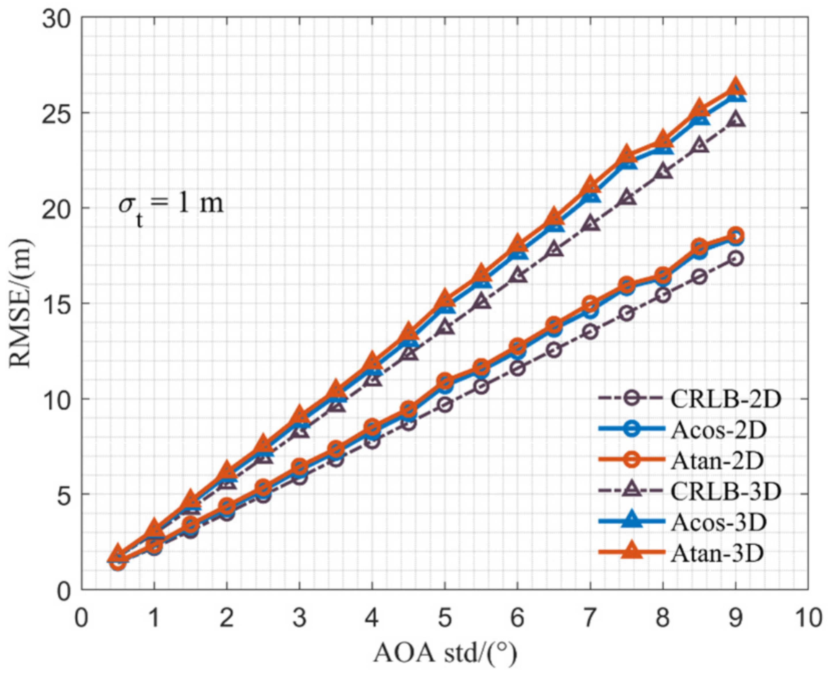
4.1. 5G RTT/AOA Parameter Settings Based on CRLB

The GPP TS38.855 [10] evaluates the performance of 5G in three distinct positioning scenarios: Urban Micro (UMi), Urban Macro (UMa), and Indoor Office, and the simulation experiment is conducted within the UMi scenario set in an urban environment. The scenario range specified in this paper was 200 × 200 m. The coordinate system chosen was the navigation coordinate system. Additionally, the positioning points were randomly distributed within the scenario covered by the base station. The height of the terminal was set to 1.5 m, with a fixed standard deviation of 1 m for ranging. The standard deviation of the angular measurement of AOAs was denoted as ${\sigma }_{\theta }={\sigma }_{\phi }$, ranging from 0 to 9 degrees with an increment of 0.5 degrees. We randomly generated simulation points by setting the noise value and the derivation part of the observation noise based on the CRLB in Appendix B. There were 18 groups of comparison experiments for angular variance of AOAs. To ensure the stability and credibility of the experimental results, 10,000 observations were randomly generated in each group of experiments.

4.2. Performance Evaluation

Firstly, the efficiency of the Acos method and the Atan method in RTT/AOA joint positioning for a single base station was compared. When using least squares to solve nonlinear problems, the convergence of the problem and the number of iterations are two distinct criteria. For this Section, the positioning success rate and the average number of iterations of the Acos and Atan methods were calculated based on 18 groups of experiments, each comprising 10,000 observations. The results are presented in

Table 1. Efficiency comparison of single-base-station positioning algorithms.

Algorithms	Success Rate	Number of Iterations
Acos	$100.00\%$	3.00
Atan	$83.11\%$	9.17

. Among the 10,000 observations, the Atan method successfully obtained convergent and correct solutions 8311 times, resulting in a positioning success rate of $83.11\%$. The average number of iterations for successfully positioned solutions was 9.17 times. In contrast, the Acos approach significantly reduced the average number of iterations to 3 and achieved a positioning success rate of $100\%$. The experiment demonstrated that the efficiency of the Acos method is significantly superior to the Atan method for solving the RTT/AOA-joint-positioning problem for a single base station.

This set of experiments also compared the localization results of the Acos method and the Atan method. The Root Mean Square Error (RMSE) of the positioning results is illustrated in Figure 3. The blue line, red line, and black line represent the variations of the Acos method, the Atan method, and the CRLB RMSE with the standard-deviation-of-angle observation. In Figure 3, the circle represents the two-dimensional positioning, the triangle represents the three-dimensional positioning, and the lower limit of the CRLB represents the variance’s lower limit achievable by the joint positioning of RTT/AOA for the single base station under the current parameter setting. As the standard-deviation-of-angle measurement increased, the trend of the six lines remained consistent, and the positioning error linearly increased. The positioning error of both the Acos method and the Atan method was greater than the lower limit of the CRLB. Notably, the Acos method exhibited slightly superior positioning errors in both two-dimensional and three-dimensional results.

To emphasize the distinctions between the Acos and Atan methods in the positioning results,

Table 2. Comparison of RTT/AOA positioning errors in a single base station.

Index	Acos-2D	Atan-2D	Acos-3D	Atan-3D
Mean Value	1.89	1.95	$2.64$	2.72
Max Value	$12.05$	12.05	$12.07$	12.07
Min Value	$0.02$	0.03	$0.11$	0.14
STD	$1.30$	1.33	$1.54$	2.72

provides a comparison of two-dimensional and three-dimensional positioning errors for 10,000 random observations at ${\sigma }_{\tau }=1$ m and ${\sigma }_{AOA}=1^{\circ }$. The table includes the mean, maximum, minimum, and standard deviation of the error, with the results of the Acos method highlighted in bold. The average two-dimensional and three-dimensional positioning errors of the Acos method were 1.85 m and 2.64 m, respectively, compared to the average positioning errors of the Atan method, which were 1.95 m and 2.72 m, indicating increases of $5.13\%$ and $2.94\%$, respectively.

Based on experiment, the Acos method performs better than the Atan method in solving the RTT/AOA-joint-positioning problem for a single base station, both in terms of solution efficiency and positioning accuracy. This demonstrates the effectiveness of the RTT/AOA solution proposed in this paper. The Acos method will continue to be used in subsequent fusion experiments.

5. 5G/GNSS Semiphysical Experiment

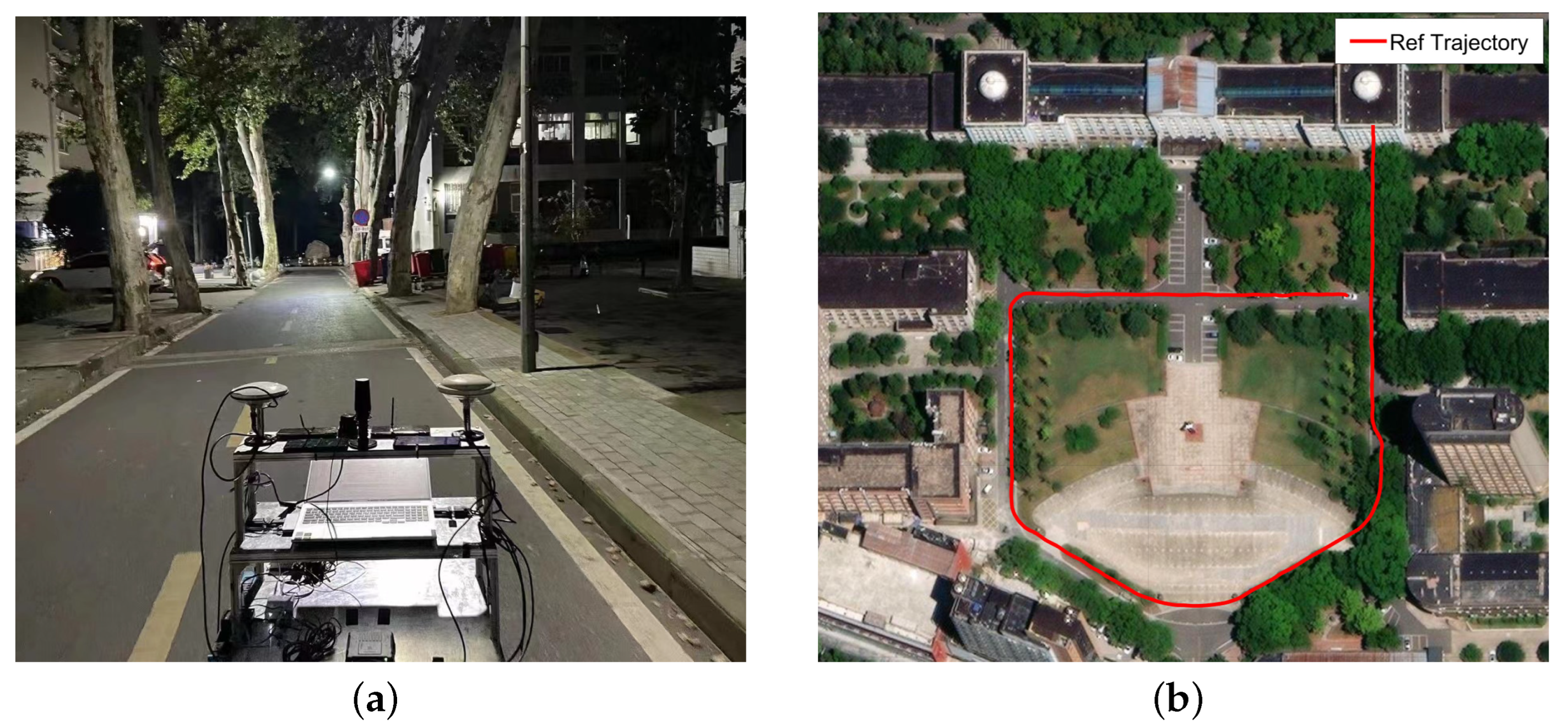
5.1. Experiment Settings

In order to verify the performance of the proposed algorithm, semiphysical experiments of GNSS in typical scenarios were carried out. GNSS data, including pseudo-range and Doppler measurements of GPS L1/L2 and BDS B1/B3 signals, were collected in Wuhan University on 1 August 2023. We calculated the real distance and angle from each preset 5G base station to the UE at each epoch and we estimated the CRLB of 5G RTT/AOA measurements by the distance-dependent noise model in Appendix B. According to the CRLB, the standard deviation of observation noise was estimated. The 5G RTT/AOA data were synthetically generated by introducing appropriate observation noise following white Gaussian noise. The reference truth value acquired through the high-precision integrated navigation system could reach centimeter-level in most scenarios and decimeter-level in a few scenarios. Figure 4a shows the measured scene, and Figure 4b shows the experimental route.

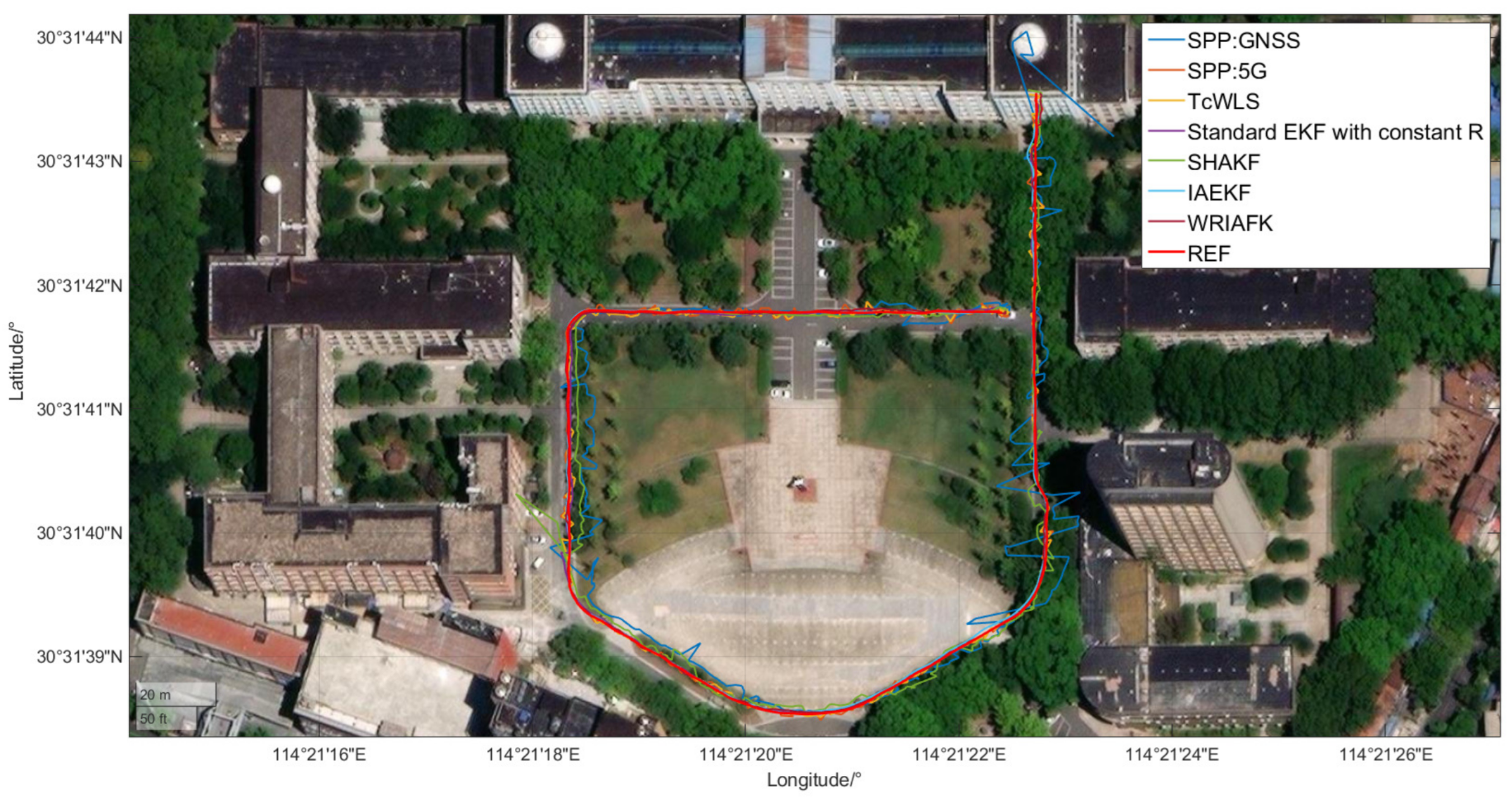
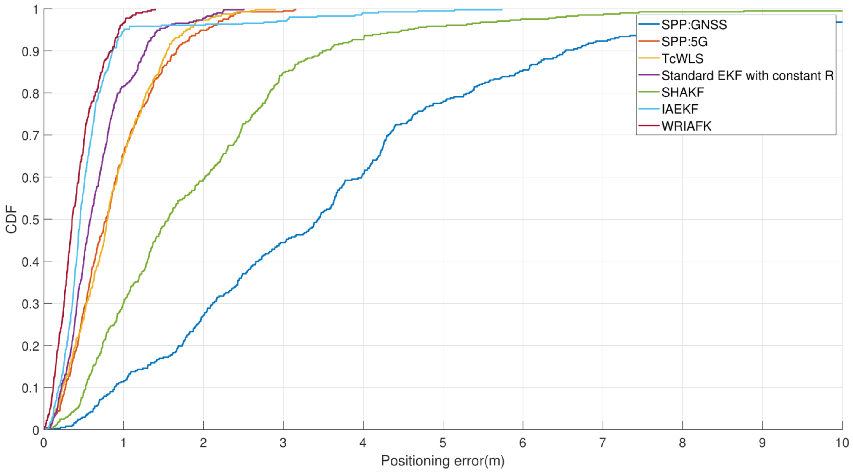
5.2. Performance Evaluation

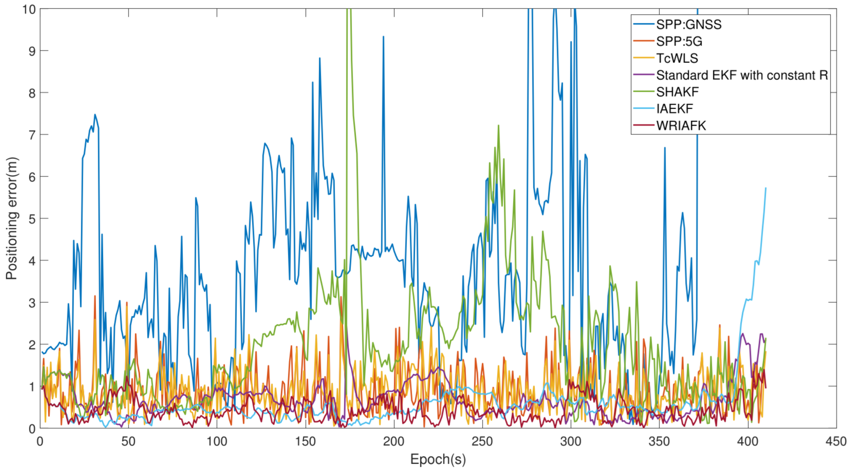
This group of experiments evaluated the gain of 5G data to the positioning system, and it compared the proposed fusion algorithm with the positioning of a single data source. Additionally, the performance of the proposed fusion algorithm was compared with common industry methods, such as standard EKF, Weighted Least Squares (WLS) [35], SHAKF, and the Innovation-based Anti-Error Kalman Filter (IAEKF) [35] to validate its effectiveness. Figure 5 illustrates the final positioning trajectory of various algorithms on the remote-sensing image map. Figure 6 presents the Cumulative Distribution Function (CDF) statistical diagram for these algorithms, while Figure 7 displays the Root Mean Square (RMS) error distribution diagram for the same set of algorithms.

Table 3. Comparison of RTT/AOA positioning errors in a single base station.

Index	SPP:GNSS	SPP:5G	TcWLS	SEKF	SHAKF	IAEKF	WRIAKF
Mean	3.78	0.89	0.86	0.68	1.96	0.60	0.42
$1\sigma (cdf68\%)$	4.26	1.07	1.04	0.79	2.39	0.58	0.50
$2\sigma (cdf95\%)$	8.24	1.95	1.79	1.45	4.56	1.00	0.94
$3\sigma (cdf99\%)$	14.23	2.99	2.58	2.24	7.45	3.99	1.15

shows the comparison of errors of each algorithm, including the average error and the error at $1\sigma /2\sigma /3\sigma$ levels. Analysis of the three graphs reveals that the 5G/GNSS-fusion positioning algorithm demonstrated enhanced performance when compared to a single data source employing the same weighted-least-squares algorithm. Among all the algorithms utilizing Kalman filtering, the SHAKF exhibited the poorest performance, with errors at $1\sigma /2\sigma /3\sigma$ levels measuring 2.38 m, 4.56 m, and 7.22 m, respectively. An examination of the adaptive noise matrix during the algorithm’s operation reveals that, in many instances, the noise matrix failed to maintain a positive definite matrix and, at times, approached singularity, which confirmed the limitations of the SHAKF algorithm proposed earlier. The standard Extended Kalman Filter algorithm outperformed the Tight Coupled Weighted Least Squares (TcWLS) [13] algorithm by considering the time correlation. However, the constant noise matrix in the system model could not adapt to changing observation conditions in dynamic environments and lacked resistance to gross errors, leading to a certain degree of accuracy loss. The Weighted Robust Iterative Adaptive Kalman Filter, as presented in this paper, exhibited the best performance. Compared to the second-best-performing IAEKF, the WRIAKF demonstrated improvements of $30\%$, $13.79\%$, and $71.18\%$ at $1\sigma /2\sigma /3\sigma$ levels, respectively. These findings thoroughly demonstrate the superiority of the proposed algorithm.

In addition, as is shown in Figure 7 and Figure 8, all kinds of temporal-filtering algorithms except SHAKF have good performance when the number of satellites is sufficient and stable. However, it is worth noting that near the trajectory terminal, due to the occlusion of buildings, the number of observable satellites decreases sharply and the observation environment changes dramatically. In such challenging conditions, the SPP fails to provide a positioning solution, and other filter-based or TcWLS algorithms are more or less affected by interference. The WRIAKF algorithm, introduced in this paper, demonstrates minimal susceptibility to these challenges, thanks to its implementation of dual gross error detection and adaptive adjustment of the forgetting factor. This substantiates that the WRIAKF algorithm consistently delivers robust localization performance even in scenarios with rapidly changing observation environments.

5.3. Discussion

When considering traditional GNSS in urban environments or amid high-rise buildings, signal blockage and frequent multipath interference often lead to inaccurate positioning. In contrast, the 5G signal harnesses its advantages of low latency, high bandwidth, and large capacity. It can provide positioning information even in intricate scenarios, such as indoor areas and urban canyons, which compensates for the shortcomings and limitations of GNSS to a certain extent. Moreover, 5G networks generally exhibit greater stability than GNSS signals. Consequently, the amalgamation of 5G and GNSS positioning confers enhanced reliability in inclement weather or challenging conditions, bearing particular significance for emergency rescue operations, traffic management, and military applications.

In practical-application scenarios, User Equipment often establishes a connection with only one base station. However, due to limitations in the number of observations and the geometric distribution, the positioning accuracy of a single base station is significantly reduced. Hence, there is a need to explore the positioning algorithms specific to 5G single base stations. Additionally, addressing the 5G-single-base-station RTT/AOA-joint-positioning challenge, a novel approach is introduced. This method involves the transformation of the arctangent trigonometric function into cosine functions, followed by linearization. This transformation mitigates the issue of high non-linearity between observation angles and position coordinates. Furthermore, the proposed algorithm’s advantages are analyzed through simulation experiments. To tackle the problems related to noise-matrix assignment in the standard EKF algorithm and the adjustment of weights between different observation systems in the absence of prior information, a fusion positioning algorithm is proposed. This algorithm leverages 5G angle, distance, GNSS pseudo-range, and Doppler measurements for adaptive Kalman filtering. Aiming at the problem of non-positivity or singularity of the noise matrix in SHAKF, this algorithm resolves by replacing the adaptive-observation noise matrix R estimation based on the prior residual with an estimation based on the posterior residual. It also introduces dual gross error detection adaptive correction of the forgetting factor based on innovation in the iterative Kalman filter to enhance accuracy and robustness. Finally, semiphysical experiments validate the proposed algorithm’s improvements in positioning accuracy and reliability.

6. Conclusions

In this study, we mainly discussed the problems of high linearization of user position and angle in the 5G RTT/AOA joint positioning of a single base station, lack of accurate prior information and assignment of observation noise under different observation conditions. In response to these problems, angle cosine and WRIAKF algorithms were proposed, respectively. The robustness and superiority of the algorithm were verified by simulation and semiphysical experiments. The numerical results showed that compared with the traditional Atan method, the Acos method reduced the average number of iterations from 9.17 to 3 with higher accuracy, which greatly improves the efficiency of the algorithm. Meanwhile, compared with the standard EKF, the WRIAKF algorithm improved by $48.66\%$, $35.17\%$, and $38.23\%$ at $1\sigma /2\sigma /3\sigma$, respectively.

References

1. Groves, P.D. Principles of GNSS, Inertial, and Multisensor Integrated Navigation Systems, 2nd ed.; Artech House: London, UK, 2013. [Google Scholar]
2. Seco-Granados, G.; López-Salcedo, J.; Jiménez-Baños, D.; López-Risueño, G. Challenges in Indoor Global Navigation Satellite Systems: Unveiling its core features in signal processing. IEEE Signal Process. Mag. 2012, 29, 108–131. [Google Scholar] [CrossRef]
3. Xu, B.; Jia, Q.; Hsu, L.T. Vector Tracking Loop-Based GNSS NLOS Detection and Correction: Algorithm Design and Performance Analysis. IEEE Trans. Instrum. Meas. 2020, 69, 4604–4619. [Google Scholar] [CrossRef]
4. Chen, R.Z.; Chen, L. Indoor Positioning with Smartphones: The State-of-the-art and the Challenges. Acta Geod. Cartogr. Sin. 2017, 46, 1316. [Google Scholar]
5. Gakne, P.V.; O’Keefe, K. Tightly-coupled GNSS/vision using a sky-pointing camera for vehicle navigation in urban areas. Sensors 2018, 18, 1244. [Google Scholar] [CrossRef] [PubMed]
6. Wen, W.W.; Hsu, L.T. 3d LiDAR aided GNSS NLOS mitigation in urban canyons. IEEE Trans. Intell. Transp. Syst. 2022, 23, 18224–18236. [Google Scholar] [CrossRef]
7. Sun, R.; Wang, J.H.; Cheng, Q.; Mao, Y.; Ochieng, W.Y. A new IMU-aided multiple GNSS fault detection and exclusion algorithm for integrated navigation in urban environments. GPS Solut. 2021, 25, 147. [Google Scholar] [CrossRef]
8. De Angelis, G.; Baruffa, G.; Cacopardi, S. GNSS/Cellular hybrid positioning system for mobile users in urban scenarios. IEEE Trans. Intell. Transp. Syst. 2012, 14, 313–321. [Google Scholar] [CrossRef]
9. Ruan, Y.L.; Chen, L.; Zhou, X.; Guo, G.Y.; Chen, R.Z. Hi-Loc: Hybrid Indoor Localization via Enhanced 5G NR CSI. IEEE Trans. Instrum. Meas. 2022, 71, 5502415. [Google Scholar] [CrossRef]
10. 3GPP TS 38.855. Study on NR Positioning Support (Release 16). Available online: https://portal.3gpp.org/desktopmodules/Specifications/SpecificationDetails.aspx?specificationId=3501 (accessed on 28 March 2019).
11. 3GPP RP-223549. New WID on Expanded and Improved Positioning. Available online: https://www.3gpp.org/ftp/Information/WI_Sheet/?sortby=daterev (accessed on 20 June 2023).
12. Destino, G.; Saloranta, J.; Seco-Granados, G.; Wymeersch, H. Performance Analysis of Hybrid 5G-GNSS Localization. In Proceedings of the 2018 52nd Asilomar Conference on Signals, Systems, and Computers, Pacific Grove, CA, USA, 28–31 October 2018; pp. 8–12. [Google Scholar]
13. Del Peral-Rosado, J.; Saloranta, J.; Destino, G.; López-Salcedo, J.; Seco-Granados, G. Methodology for simulating 5G and GNSS highaccuracy positioning. Sensors 2018, 18, 3220–3244. [Google Scholar] [CrossRef] [PubMed]
14. Abu-Shaban, Z.; Seco-Granados, G.; Benson, C.R.; Wymeersch, H. Performance analysis for autonomous vehicle 5G-assisted positioning in GNSS-challenged environments. In Proceedings of the 2020 IEEE/ION Position, Location and Navigation Symposium (PLANS), Portland, OR, USA, 20–23 April 2020; pp. 996–1003. [Google Scholar]
15. Del Peral-Rosado, J.; Bartlett, D.; Grec, F.; Ries, L.; Chassaigne, A. Physical-layer abstraction for hybrid GNSS and 5G positioning evaluations. In Proceedings of the 2019 IEEE 90th Vehicular Technology Conference (VTC2019-Fall), Honolulu, HI, USA, 22–25 September 2019; pp. 1–6. [Google Scholar]
16. Sun, C.; Zhao, H.; Bai, L.; Cheong, J.W.; Dempster, A.G.; Feng, W. GNSS-5G hybrid positioning based on TOA/AOA measurements. In Proceedings of the China Satellite Navigation Conference (CSNC) 2020, Chengdu, China, 22–25 November 2020; pp. 527–537. [Google Scholar]
17. Hiltunen, T.; Turkka, J.; Mondal, R.; Ristaniemi, T. Performance evaluation of LTE radio fingerprint positioning with timing advancing. In Proceedings of the 2015 10th International Conference on Information, Communications and Signal Processing (ICICS), Singapore, 2–4 December 2015; pp. 1–5. [Google Scholar]
18. Ruan, Y.; Chen, L.; Zhou, X.; Liu, Z.; Liu, X.; Guo, G. iPos-5G: Indoor Positioning via Commercial 5G NR CSI. IEEE Internet Things J. 2023, 10, 8718–8733. [Google Scholar] [CrossRef]
19. Zhou, X.; Chen, L.; Ruan, Y.L. Indoor Positioning with Multibeam CSI From a Single 5G Base Station. IEEE Sens. Lett. 2024, 8, 1. [Google Scholar] [CrossRef]
20. Zhou, X.; Chen, L.; Ruan, Y.L.; Chen, R.Z. Indoor positioning with multi-beam CSI of commercial 5G signals. Urban Inf. 2024, 3, 1. [Google Scholar] [CrossRef]
21. Guo, C.; Qi, S.; Guo, W.; Deng, C.; Liu, J. Structure and performance analysis of fusion positioning system with a single 5G station and a single GNSS satellite. Geo-Spat. Inf. Sci. 2023, 26, 94–106. [Google Scholar] [CrossRef]
22. He, J.; Swamy, M.N.S.; Ahmad, M.O. Efficient Application of MUSIC Algorithm Under the Coexistence of Far-Field and Near-Field Sources. IEEE Trans. Signal Process. 2012, 60, 2066–2070. [Google Scholar] [CrossRef]
23. Wang, B.; Zhao, Y.; Liu, J. Mixed-Order MUSIC Algorithm for Localization of Far-Field and Near-Field Sources. IEEE Signal Process. Lett. 2013, 20, 311–314. [Google Scholar] [CrossRef]
24. Zheng, Z.; Fu, M.; Wang, W.-Q.; So, H.C. Mixed Far-Field and near-Field Source Localization Based on Subarray Cross-Cumulant. Signal Process. 2018, 150, 51–56. [Google Scholar] [CrossRef]
25. Zhou, X.; Chen, L.; Yan, J.; Chen, R.Z. Accurate DOA Estimation with Adjacent Angle Power Difference for Indoor Localization. IEEE Access 2020, 8, 44702–44713. [Google Scholar] [CrossRef]
26. Shahmansoori, A.; Garcia, G.E.; Destino, G.; Seco-Granados, G.; Wymeersch, H. Position and Orientation Estimation Through Millimeter-Wave MIMO in 5G Systems. IEEE Trans. Wirel. Commun. 2018, 17, 1822–1835. [Google Scholar] [CrossRef]
27. Abdallah, A.A.; Shamaei, K.; Kassas, Z.M. Assessing Real 5G Signals for Opportunistic Navigation. In Proceedings of the 33rd International Technical Meeting of the Satellite Division of The Institute of Navigation (ION GNSS+ 2020), Online, 22–25 September 2020; pp. 2548–2559. [Google Scholar]
28. Liu, Z.L.; Chen, L.; Zhou, X.; Jiao, Z.H.; Guo, G.Y.; Chen, R.Z. Machine Learning for Time-of-Arrival Estimation with 5G Signals in Indoor Positioning. IEEE Internet Things J. 2023, 10, 9782–9795. [Google Scholar] [CrossRef]
29. Liu, Q.; Liu, R.; Wang, Z.; Zhang, Y. Simulation and Analysis of Device Positioning in 5G Ultra-Dense Network. In Proceedings of the 2019 15th International Wireless Communications & Mobile Computing Conference (IWCMC), Tangier, Morocco, 24–28 June 2019; pp. 1529–1533. [Google Scholar]
30. Dev, C.S.G.N.; Pathak, L.; Ponnamareddy, G.; Das, D. NRPos: A Multi-RACH Framework for 5G NR Positioning. In Proceedings of the 2020 IEEE 3rd 5G World Forum (5GWF), Bangalore, India, 10–12 September 2020. [Google Scholar]
31. Rahman, M.M. Investigations of 5G Localization with Positioning Reference Signals. Available online: https://trepo.tuni.fi/handle/10024/120011 (accessed on 3 June 2021).
32. Ferre, R.; Seco-Granados, G.; Lohan, E. Positioning Reference Signal Design for Positioning via 5G. Available online: https://www.ursi.fi/2019/Papers/Morales.pdf (accessed on 3 June 2021).
33. Liu, J.; Deng, Z.; Hu, E.; Huang, Y.; Deng, X.; Zhang, Z.; Ding, Z.; Liu, B. GNSS-5G Hybrid Positioning Based on Joint Estimation of Multiple Signals in a Highly Dependable Spatio-Temporal Network. Remote Sens. 2023, 15, 4220. [Google Scholar] [CrossRef]
34. Bai, L.; Sun, C.; Dempster, A.G.; Zhao, H.; Cheong, J.W.; Feng, W. GNSS-5G Hybrid Positioning Based on Multi-Rate Measurements Fusion and Proactive Measurement Uncertainty Prediction. IEEE Trans. Instrum. Meas. 2022, 71, 8501415. [Google Scholar] [CrossRef]
35. Mohamed, A.H.; Schwarz, K.P. Adaptive Kalman Filtering for INS/GPS. J. Geod. 1999, 73, 193–203. [Google Scholar] [CrossRef]
36. Karasalo, M.; Hu, X. An Optimization Approach to Adaptive Kalman Filtering. In Proceedings of the 48th IEEE Conference on Decision and Control (CDC) Held Jointly with 2009 28th Chinese Control Conference, Shanghai, China, 15–18 December 2009. [Google Scholar]
37. Akhlaghi, S.; Zhou, N.; Huang, Z. Adaptive Adjustment of Noise Covariance in Kalman Filter for Dynamic State Estimation. In Proceedings of the 2017 IEEE Power & Energy Society General Meeting, Chicago, IL, USA, 16–20 July 2017. [Google Scholar]
38. Mehra, R. Approaches to Adaptive Filtering. IEEE Trans. Autom. Control. 1972, 17, 693–698. [Google Scholar] [CrossRef]
39. Bierman, G. Stochastic Models, Estimation, and Control. IEEE Trans. Autom. Control. 1983, 28, 868–869. [Google Scholar] [CrossRef]
40. Sage, A.P.; Husa, W. Adaptive Filtering with Unknown Prior Statistics. In Proceedings of the Joint Automatic Control Conference, Washington, DC, USA, 22–24 June 1969; pp. 760–769. [Google Scholar]
41. Yang, Y.X.; Cheng, M.K.; Shum, C.K.; Tapley, B.D. Robust estimation of systematic errors of satellite laser range. J. Geod. 1999, 73, 345–349. [Google Scholar] [CrossRef]
42. Ho, K.C.; Lu, X.N.; Kovavisaruch, L. Source localization using TDOA and FDOA measurements in the presence of receiver location errors: Analysis and solution. IEEE Trans. Signal Process. 2007, 55, 684–696. [Google Scholar] [CrossRef]
43. Pauluzzi, D.R.; Beaulieu, N.C. A comparison of SNR estimation techniques for the AWGN channel. IEEE Trans. Commun. 2000, 48, 1681–1691. [Google Scholar] [CrossRef]
44. Abu-Shaban, Z.; Zhou, X.; Abhayapala, T.; Seco-Granados, G.; Wymeersch, H. Error bounds for uplink and downlink 3D localization in 5G millimeter wave systems. IEEE Trans. Wirel. Commun. 2018, 17, 4939–4954. [Google Scholar] [CrossRef]
45. MacCartney, G.R.; Zhang, J.H.; Nie, S.; Rappaport, T.S. Path Loss Models for 5G Millimeter Wave Propagation Channels in Urban Microcells. In Proceedings of the IEEE Global Communications Conference (GLOBECOM), Atlanta, GA, USA, 9–13 December 2013; pp. 3948–3953. [Google Scholar]
Figure 1. Basic principle of RTT.
Remotesensing 16 01009 g001
Figure 2. Implementation flowchart of the SHAKF, where d k = ( 1 b ) / ( 1 b k + 1 ) is the amnestic factor and b is the forgetting factor usually chosen in the range from 0.95 to 0.99.
Remotesensing 16 01009 g002
Figure 3. RMSE comparison of single-base-station positioning algorithms over an area of 200 by 200 m.
Remotesensing 16 01009 g003
Figure 4. Scene and trajectory: (a) Measured scene. (b) Experiment trajectory.
Remotesensing 16 01009 g004
Figure 5. Positioning trajectory of various algorithms.
Remotesensing 16 01009 g005
Figure 6. CDF statistical diagram for these algorithms.
Remotesensing 16 01009 g006
Figure 7. RMSE comparison of the algorithms.
Remotesensing 16 01009 g007
Figure 8. Number of visible GPS/BDS satellites varying over time.
Remotesensing 16 01009 g008