Abstract
The construction of a high-precision geomagnetic map is a prerequisite for geomagnetic navigation and magnetic target-detection technology. The Kriging interpolation algorithm makes use of the variogram to perform linear unbiased and optimal estimation of unknown sample points. It has strong spatial autocorrelation and is one of the important methods for geomagnetic map construction. However, in a region with a complex geomagnetic field, the sparse geomagnetic survey lines make the ratio of line-spacing resolution to in-line resolution larger, and the survey line direction differs from the geomagnetic trend, which leads to a serious effect of geometric anisotropy and thus, reduces the interpolation accuracy of the geomagnetic maps. Therefore, this paper focuses on the problem of geometric anisotropy in the process of constructing a geomagnetic map with sparse data, analyzes the influence of sparse data on geometric anisotropy, deduces the formula of geometric anisotropy correction, and proposes a modified interpolation algorithm accounting for geometric anisotropy correction of variogram for sparse geomagnetic data. The results of several sets of simulations and measured data show that the proposed method has higher interpolation accuracy than the conventional spherical variogram model in a region where the geomagnetic anomaly gradient changes sharply, which provides an effective way to build a high-precision magnetic map of the complex geomagnetic field under the condition of sparse survey lines.
1. Introduction
As a basic work of geomagnetic matching navigation and magnetic anomaly detection, the geomagnetic map is of great significance to improve navigation accuracy and target-detection ability. Geomagnetic mapping can be obtained by means of aeromagnetic survey, etc. According to relevant measurement specifications [1,2,3,4,5], the magnetic data obtained by aeromagnetic survey is characterized by dense data in the direction of survey lines and sparse data in the direction of line-spacing. Such data cannot be directly used for geomagnetic navigation and magnetic target detection, and it is necessary to interpolate the data to establish high-resolution grid data. The Kriging interpolation algorithm is one of the best methods. Kriging uses a variogram to perform linear unbiased and optimal estimation of unknown sample points, and it has strong spatial autocorrelation, which can better represent the structural component of the geomagnetic field and accurately reflect the geomagnetic information in a local region [6]. Hao et al. [7] studied the basic principle of ordinary Kriging interpolation and found that the accuracy of geomagnetic grid data obtained using it is higher than that obtained by inverse distance weighting interpolation, natural neighbor interpolation and other methods. Yang et al. [8] used cross-validation to verify that the universal Kriging method has better interpolation effect than the ordinary Kriging method. Cai et al. [9] applied the co-Kriging interpolation algorithm to indoor navigation and positioning based on the geomagnetic field. The sample was divided into two parts for ordinary Kriging interpolation processing and then fusion processing, which has the characteristics of small root-mean-square error and good interpolation effect. At the same time, with the development of deep learning technology, Zhao et al. [10] combined neural networks with a Kriging interpolation algorithm and proposed a geomagnetic reference map construction method based on the combination of Kriging and a back propagation (BP) neural network. The Kriging interpolation error in a large gradient region is greater than that in a BP neural network, and the interpolation error in a small gradient region is smaller than that in a BP neural network. In the large gradient region, the predicted value of the BP neural network is used instead of the Kriging interpolation result to improve the interpolation accuracy.
However, the sparsity of aeromagnetic data and the direction of survey line intensify the influence of geometric anisotropy on the accuracy of geomagnetic map construction, which shows that the geomagnetic detail with high resolution in-line cannot be distinguished with low resolution in the line-spacing direction. Wackernagel et al. [11], Sun [12] and Mcbratney et al. [13] point out that anisotropy is absolute and isotropy is relative. However, geometric anisotropy is often ignored in the actual processing, so the accuracy of interpolation is reduced by processing according to isotropy. Therefore, this paper analyzes the geometric anisotropy problem of sparse data, deduces the geometric anisotropy processing formula, and proposes a modified interpolation algorithm accounting for geometric anisotropy correction of variogram for sparse geomagnetic data. Based on the simulated data and the measured data, the proposed algorithm is used to construct high-precision geomagnetic maps respectively, and is compared with the geomagnetic maps constructed using a spherical variogram model. The results show that the interpolation accuracy of this method has obvious advantages, which greatly reduces the maximum absolute error, average absolute error and root-mean-square error, and is suitable for constructing local geomagnetic reference maps with high precision and high resolution.
2. Influence Analysis of Geometric Anisotropy of Variogram
2.1. Principles of Kriging Interpolation Algorithm
The Kriging interpolation algorithm is a spatial interpolation method based on geostatistics, which makes a minimum variance estimation and linear unbiased method for unknown data of similar characteristics in a region, according to certain characteristic data of several information samples.
2.1.1. Regionalized Variable
The magnetic data provide information about regionalized variables, which are simply functions (of a spatial or time continuum) whose behavior we would like to characterize. In the probabilistic model, a regionalized variable is considered to be a realization of a random function (the infinite family of random variables constructed at all points x. of a spatial domain). The advantage of this approach is that we shall only try to characterize the random function and not a particular regionalized variable. In such a setting, the data values are samples from one particular realization of [11].
2.1.2. Principle of Interpolation
The basic idea of the Kriging algorithm is that a certain weight is assigned to each sample value, according to the spatial correlation between sample points, especially the spatial position, and the unknowns in the estimation region that were estimated using the weighted average method [14].
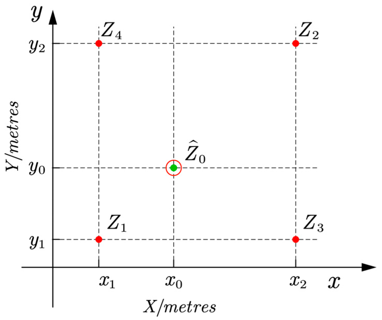
As shown in Figure 1, (the red points) is a set of measured magnetic field sample data points with coordinate position , and the estimated value (the green point) of a prediction point with coordinate position can be expressed by linear combination of sampled magnetic field samples:
where is the weight of the measured point , is called the Kriging estimation of . As long as the weight coefficient is determined, the forecast point estimation can be obtained. Kriging interpolation estimation is used to calculate the weight under the condition that the estimate is unbiased and the estimation variance is minimum.
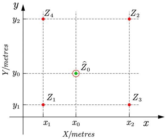
Figure 1.
Schematic diagram of Kriging interpolation algorithm.
2.1.3. Variogram
The variogram is the core of the Kriging interpolation algorithm and is defined as half of the variance of the difference of the regionalized variable at two points , and the formula is:
where is the variogram, and is the lag distance. There are many variogram models, such as the spherical, which is more commonly used; its general form is as follows:
where is the nugget, which is the value of the variogram, when the lag is 0; is the sill, which is defined as the value reached when the variogram is in a stable state with the increase of lag ; is the arch height, which is defined as the difference between sill and nugget; is the range, which is defined as the size of the autocorrelation range of regionalized variables.
2.1.4. Experimental Variogram
The experimental variogram is an estimate of the variogram constructed from the measured data. We can divide every pair of data: is respectively regarded as a one-time implementation of , represents the groups of the data pair divided by the vector , so the formula of the experimental variogram is obtained:
For different lags , the values of can be calculated according to Equation (4), and points can be marked in the graph of experimental variogram, which can directly reflect the relevant situation of measurement data [11].
2.2. Analysis of Geometric Anisotropy of Experimental Variogram
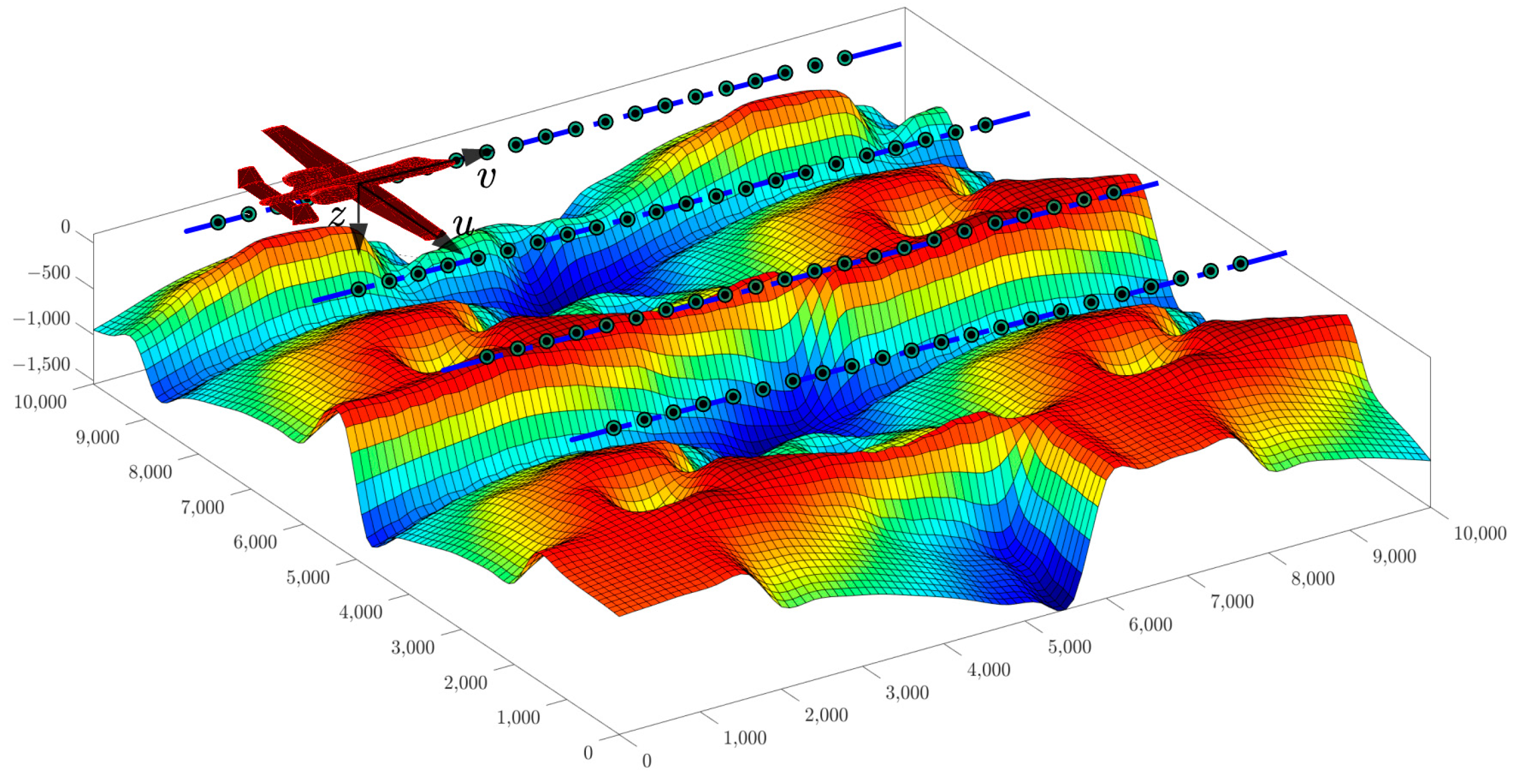
The constructed geomagnetic map is a two-dimensional plane with the height as the constant value, and as the coordinate axes, and its surveying simulation is shown in Figure 2. The and axes, which are perpendicular to each other, represent the direction in the flight-line and the direction of line-spacing during aeromagnetic measurement, and the circles with black dot are the sampling points. The magnetic data value is a regionalized variable, and the selected experimental variogram (such as spherical variogram) diagram can be drawn by sample points in Figure 3. and are the variables in different directions of the and axis, and is the anisotropy ratio. When , the direction of and axes is isotropic; when , (the blue solid line in Figure 2) or indicates the direction of and axes is anisotropic. Its physical meaning is: the average degree of variation between two points with a distance of in the direction of is equal to that with a distance of in the direction of , that is, .

Figure 2.
Simulation diagram of aeromagnetic survey flight.
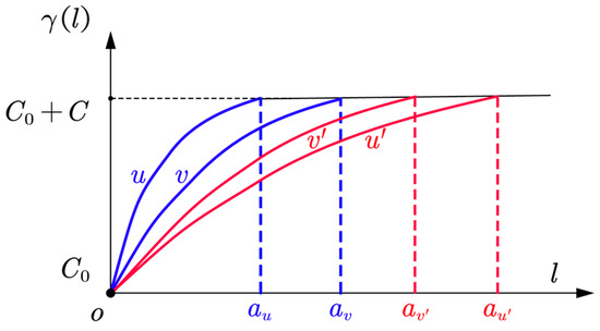
Figure 3.
Diagram of the geometric anisotropic variogram.
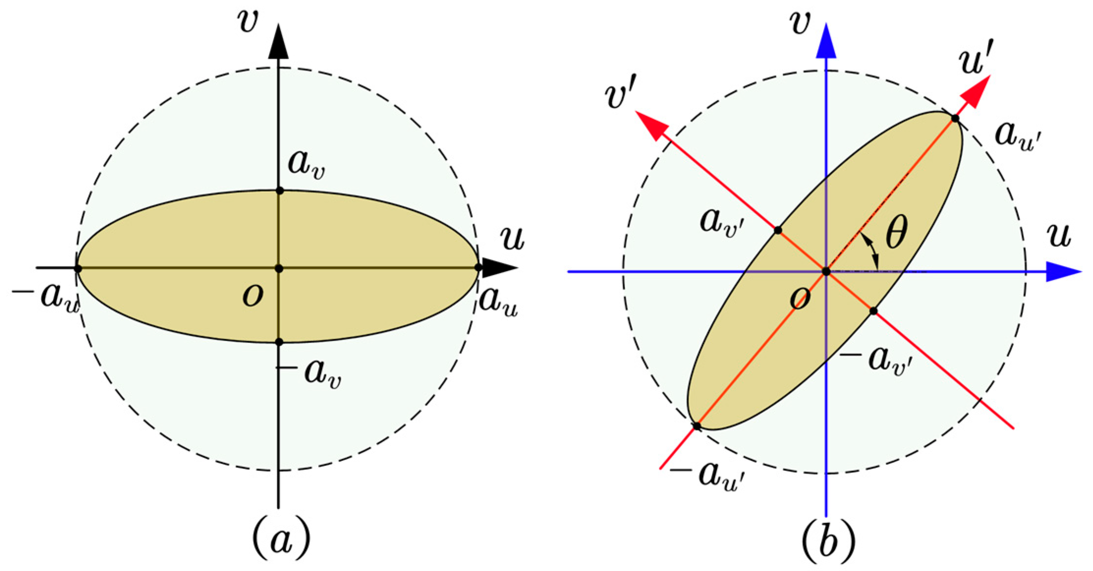
Using this variogram model, the diagram of direction–range is shown in Figure 4a. When , the direction of and axes is isotropic, the graph of direction–range is approximately a circle with range (or ) as the radius, which is shown by the dotted line in Figure 4a. When , the direction of and axes is anisotropic, the graph of direction–range is approximately an ellipse with range as the long radius and as the short radius, which is shown by the solid line in Figure 4a. This can be understood as meaning that the characteristic direction of the geomagnetic data is inconsistent with the mapping direction. If the azimuth angle between the geomagnetic variation trend and the measured axis is , then the variogram diagram and the direction–range diagram will change due to the introduction of . The converted variogram diagram is shown by the red line in Figure 3, and the converted direction–range diagram is shown by the solid line in Figure 4b. The red and blue lines in Figure 3 correspond to the red and blue lines in Figure 4b, indicating the transformation of the coordinate system from Coordinate to Coordinate .
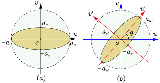
Figure 4.
Direction–range diagrams of two-dimensional geometric anisotropy. (a) Direction-range diagram of geometric anisotropy versus anisotropy; (b). Direction-range diagram of the azimuth angle between the geomagnetic variation trend and the measured axis.
Therefore, the results of geomagnetic data interpolation are not only related to the length of lag, but also to the direction of lag. If the trend of geomagnetic change is the same as the change of lag distance in all directions, then it is isotropic. If the geomagnetic trend is not the same as the change of the lag distance in each direction, it shows geometric anisotropy. This is caused by the different evolution of underlying physical processes in space [15].
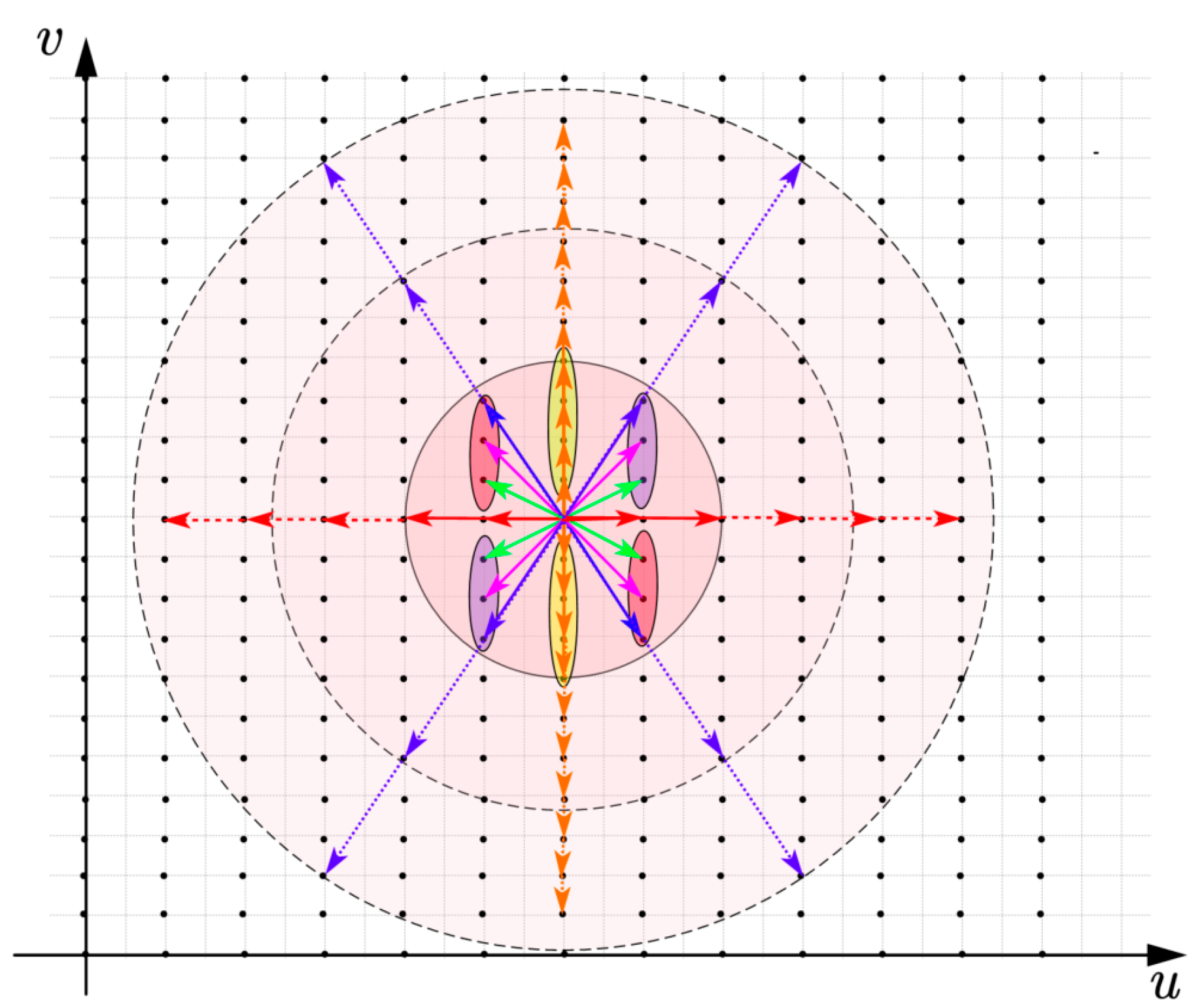
For sparse geomagnetic data, using an isotropic interpolation method to process anisotropic geomagnetic data has a great impact on the interpolation accuracy. For further explanation, this paper draws the interpolation processing diagram using the known sampling points, as shown in Figure 5. The figure shows the variable range and orientation relationship between the center point and other points in the effective region (the big pink circle region); the black dots represent the sampling points; the sampling mode along the and directions is to simulate the sampling mode between the line-spacing direction ( direction) and the flight-line direction ( direction) during aeromagnetic survey in Figure 2; and the sampling points along the direction are
twice the number of sampling points along the direction to simulate the sparsity of geomagnetic data. Although two times is a small percentage, it is just one way of analyzing the problem.
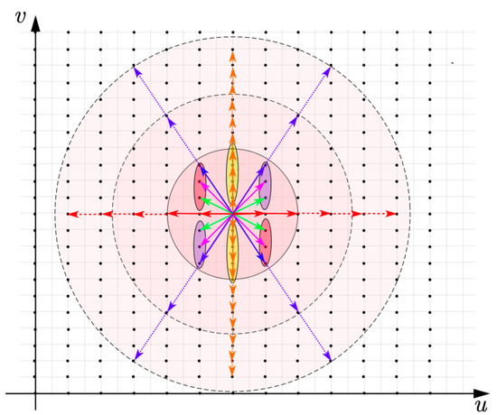
Figure 5.
Diagram of data interpolation processing.( The different colors arrows represent the lag from the midpoint to the different directions.)
It can be seen from Figure 5 that: (a) through the length of the arrows of different colors, the size of the interval between the center point and the sampling points in each direction changes with the change of the direction angle; and (b) by setting the effective region between two points (the large, medium and small regions of the pink circle), the number of sampling points in each direction around the central point decreases with the reduction of the effective region, and some directions even have no sample points.
It can be determined from Figure 5 that:
- (1)
- If the geomagnetic trend is distributed along the direction (orange arrows), the number of sampling data is sufficient and the interval is small, thus the resolution is high and the magnetic trend in this direction can be better represented;
- (2)
- If the geomagnetic trend is distributed along the direction (red arrows), the number of sampling data and interval are significantly lower than that along the direction , which can properly reflect the geomagnetic trend in this direction. If the sampling interval in this direction is increased, and the data become more and more sparse, its resolution will be reduced and the interpolation accuracy will be reduced, too;
- (3)
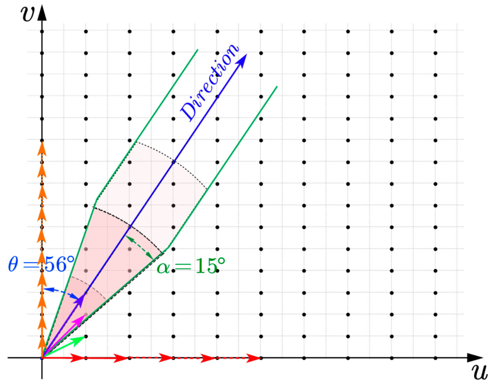
- If the geomagnetic trend is distributed along the blue line, the number of sampling points in this direction is extremely reduced (the number of blue arrows), and the sampling interval is significantly larger than the above two methods, which makes the details of geomagnetic changes in this direction easy to be ignored, thus reducing the accuracy of interpolation. At this time, in order to increase the number of samples, the area in the azimuth direction is often expanded by setting the tolerance in the azimuth direction and the lag distance tolerance, as shown in Figure 6 for the blue direction expansion in Figure 5, where the azimuth angle and the azimuth tolerance .
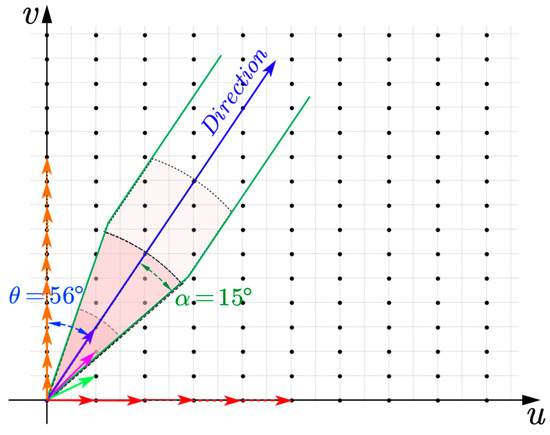 Figure 6. Diagram of azimuth angle and azimuth tolerance calculation in the interpolation processing.
The Figure 5 and Figure 6 show the method of sample point selection before the calculation of variogram parameters in the interpolation processing of geomagnetic data, which directly affects the calculation of the experimental variogram. As can be seen from Figure 6, during the measurement process, the recommended direction of the survey line is consistent with the trend of local geomagnetic change, and the actual sampling points are dense and the lag distance is small, which can better reflect the geomagnetic change in a small area. However, in the actual measurement process, it is difficult to match the geomagnetic trend, and the size of the interval between lines in direction is 8–10 times that in direction , thus increasing the influence of geometric anisotropy on the geomagnetic construction accuracy. Therefore, this paper proposes a geomagnetic map construction algorithm based on geometric anisotropy correction of variogram, by calculating the variogram in each direction of the layout area and searching for the variogram in the direction that best fits the trend of the geomagnetic map to be processed to improve the interpolation accuracy of the geomagnetic data.
3. Construction Method of Geomagnetic Map Based on Geometric Anisotropy Correction of Variogram
The geometric anisotropic variogram is a universal problem, which has a greater impact on sparse geomagnetic data. In this section, a geomagnetic interpolation algorithm based on geometric anisotropy correction of variogram is proposed by deducing the geometric anisotropy correction formula, which provides effective support for the construction of high-precision geomagnetic maps.
3.1. Geometric Anisotropy Correction Formula
For the geometric anisotropy mentioned in Section 2.2, the relevant formulas can be deduced into the following two cases:
- The characteristic direction of the geomagnetic map is consistent with the surveying direction
At this time, the diagram of direction–range is shown by the solid line in Figure 4a. Using the sample data, the range in different directions are calculated respectively, and then updated by the following formula:
where anisotropy ratio .
- 2.
- The characteristic direction of the geomagnetic map is inconsistent with the surveying direction
At this time, the diagram of direction–range is shown in Figure 4b. The surveying direction (selected axis) is at the azimuth angle to the characteristic direction of the geomagnetic data (elliptic principal axis). The processing goes through three processes of coordinate rotation, anisotropy processing and coordinate restoration in turn. For the convenience of calculation, it is converted into matrix form and solved as follows:
where is the rotation matrix, ; is the coordinate system transformation matrix, ; is the anisotropic processing matrix, ; ; is the coordinate system to restore the matrix, then
Suppose , , , then bring them into formula (7).
From formula (8), when , it is geometric isotropy; when , , it is equal to formula (5), in which the characteristic direction of the geomagnetic map is consistent with the mapping direction.
3.2. Geomagnetic Interpolation Algorithm Based on Geometric Anisotropy Correction of Variogram
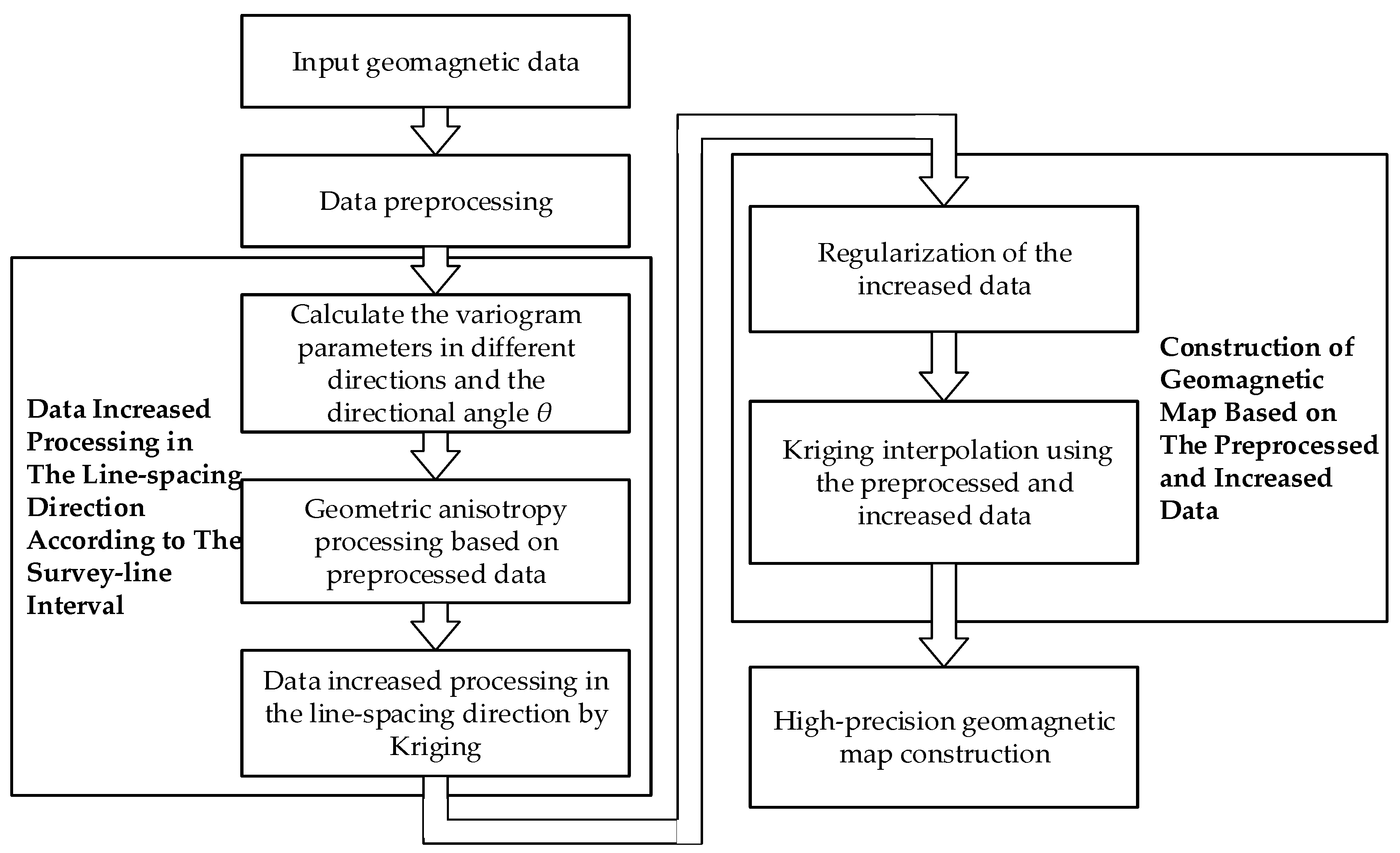
In the previous section, the geometric anisotropy correction formula was deduced. Based on this formula, a modified interpolation algorithm for sparse geomagnetic data is proposed in this section, and its flow chart is shown in Figure 7.
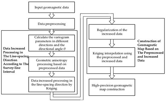
Figure 7.
Geomagnetic interpolation processing flow chart based on geometric anisotropy correction of variogram.
As shown in Figure 7, the algorithm mainly consists of two steps: data increase processing in the direction perpendicular to the line using the flight-line interval and construction of the magnetic map using the increased and raw magnetic data.
- (1)
- Data Increase Processing
According to the above sparse data survey methods, the aeromagnetic data are dense in the survey-line and sparse in the line-spacing direction, which is perpendicular to the survey-line. This step is used to increase sparse data in the line-spacing direction with the same resolution as in the survey-line, at which point a grid is constructed to reduce the effects of geometric anisotropy in both directions.
(1) According to the distribution of surveying data, the interval of the survey-line is meters, the interval of the line-spacing is meters, and the number of the increased rows between line-spacing is calculated using equation , in which is the number of the increased rows.
(2) Calculate the angle between the trend analysis of the regional geomagnetic field and the mapping direction and construct the variogram. In this paper, the brute force search method is used for processing, which mainly includes three steps: First, calculate the corresponding parameters of the variogram using Equation (3), and the range obtained is. Secondly, calculate the corresponding parameters of the variogram in each direction using Formula (3), too. The range obtained at this time is, so as to calculate the anisotropy ratios in each direction. Finally, the variogram curves of each direction and sample points are drawn in the same variogram diagram to find out which curve better fits the distribution requirements of the sample points; its corresponding azimuth angle is the appropriate one, and its corresponding parameters are the desired curve. In this paper, the initial value of the azimuth angle is set to 0°, the maximum value is 180°, and the step angle is 5° (or 6°).
(3) Based on the results of calculated in the previous step, calculate the magnetic values of the column data obtained in the first step using Kriging interpolation processing through Equations (3) and (10), so as to obtain the increased geomagnetic map data.
- (2)
- Construction of Geomagnetic Map
Using the increased data and known data as the sample, the data at this time fits a regular grid. Next, the Kriging method is used to fit it again, according to the required resolution, so as to construct high-precision geomagnetic map data. Specific methods can be referred to in Oliver [16].
In short, in order to construct the high-precision geomagnetic map, this paper first uses geometric anisotropy correction to increase the number of sparse data, and then uses the regular grid sample data composed of the known data and the increased data to interpolate again, according to the required resolution through the Kriging algorithm.
4. Simulation
According to Chen et al. [17], the simulation of the magnetic field is obtained using the mathematical expression of the field source with regular geometry distributed in space, such as the sphere model. This paper uses the sphere magnetic source model (referred to as the sphere combination model) to calculate, and the magnetic anomaly expression generated by a single sphere magnetic source is as follows:
where represents the vacuum permeability; represents the deflection angle of the magnetization intensity; and indicates the inclination of the geomagnetic field and the inclination of magnetization intensity. represents the magnetic moment, which has a relationship with the magnetic susceptibility :, represents the radius of the sphere. represents the magnetic anomaly at the position point , the variable is calculated by the formula , , and represents the center coordinates of the sphere.
4.1. Simulation of Geomagnetic Field Using Two Magnetic Dipoles
In order to verify the universality of the calculation, two magnetic dipoles are used to simulate the local geomagnetic anomaly region which is shown in Figure 8a. The parameters are shown in Table 1. The z-axis is specified as the positive direction, the normal field of geomagnetic background is set to 48,000 nT, and the true value of the simulated geomagnetic map with a regional resolution of 50 × 50 m is generated according to the relevant parameters. The magnetic data distribution shown in Figure 8b was obtained by aeromagnetic survey, where the spacing-line interval was 1000 m and the in-line interval was 250 m.
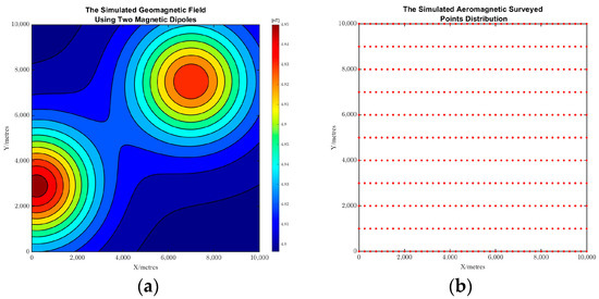
Figure 8.
Diagrams of the simulated geomagnetic map with two magnetic dipoles and simulated aeromagnetic measurement points. (a) The simulated geomagnetic map with two magnetic dipoles. (b) Diagram of the simulated aeromagnetic measurement points distribution.

Table 1.
Parameters of two magnetic dipoles.
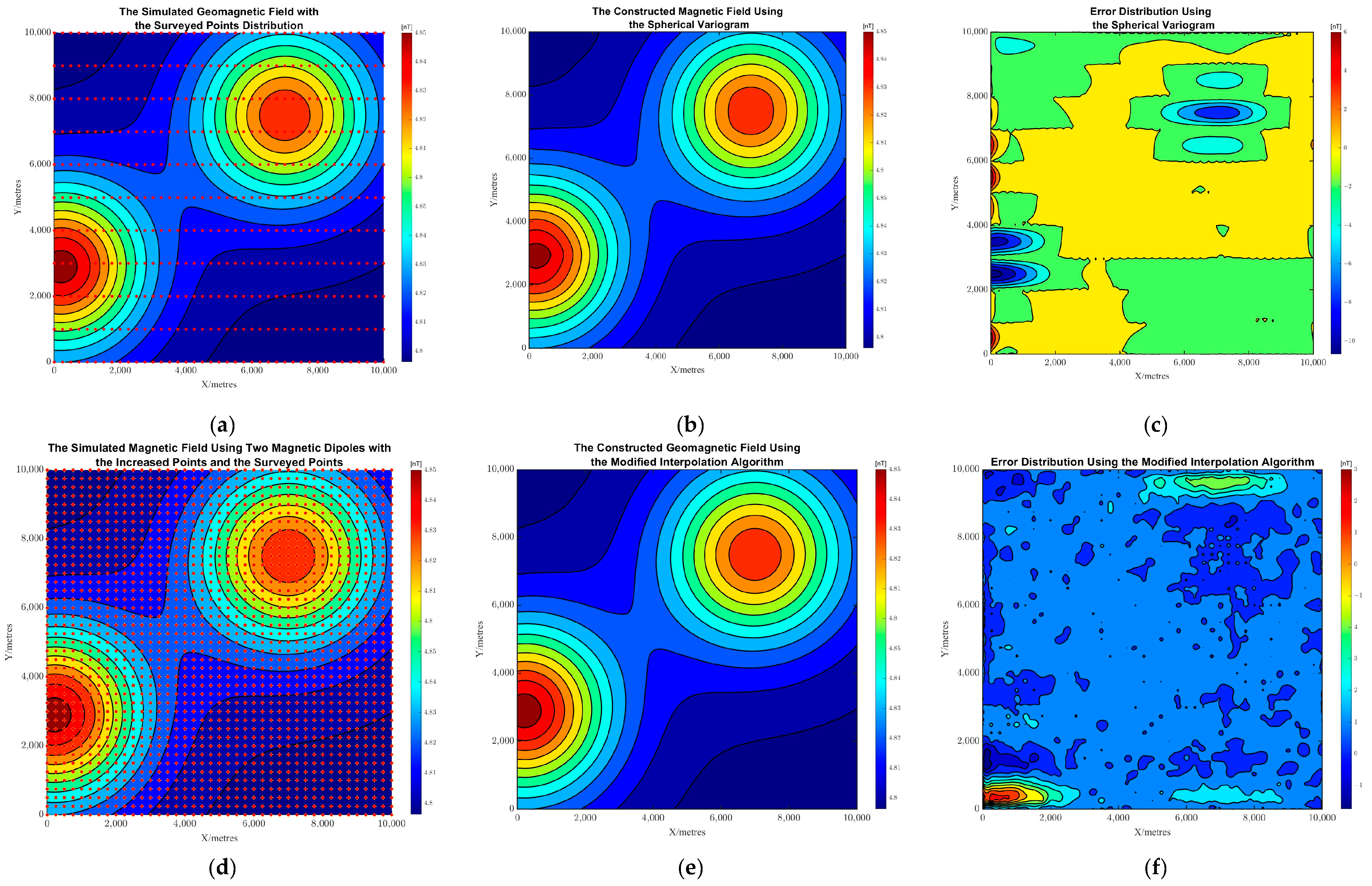
As can be seen from Figure 9a, the trend of the geomagnetic map is about 34° upward along the X direction, by calculating the relative position of two magnetic dipoles’ points (200, 2900) and (7000, 7500). Through data increase processing, the modified algorithm selected azimuth angle 35° to be the most suitable for geometric anisotropy processing. As mentioned above, it is necessary to increase the data of four routes, as shown in Figure 9d. After processing the data with the algorithm proposed in this paper, the results are shown in Figure 9e, and the comparison results between simulation diagram and interpolation diagram are shown in Figure 9f. At the same time, to verify the effectiveness of the algorithm, we use the traditional spherical variogram to process it, and the results are shown in Figure 9b. The comparison results between the simulation graph and the interpolation graph are shown in Figure 9c.

Figure 9.
A series of diagrams of the simulated geomagnetic map with two magnetic dipoles interpolated by the geometric anisotropy correction algorithm of variogram: (a) diagram of sample data distribution; (b) interpolation map processed by the traditional spherical variogram; (c) comparison results between the simulation map and the interpolation map by the traditional spherical variogram; (d) diagram of increased data distribution; (e) interpolation map processed by the geometric anisotropy correction algorithm of variogram; (f) comparison results between the simulation map and the interpolation map by the geometric anisotropy correction algorithm of variogram.
At the same time, in order to verify the effectiveness of the algorithm, we use the maximum absolute error (ME), the mean absolute error (MAE), and the root-mean-square error (RMSE) to evaluate the accuracy. ME responses are the magnitude of the error and MAE and RMSE response distribution of the error; they are calculated as shown in Equation (10).
where the parameter is the number of points in Kriging interpolation, the parameter is the true value of the magnetic field, and the parameter is the magnetic value after interpolation. From the comparison (as shown in Table 2), it can be seen that the ME, MAE, and RMSE of the improved variogram have decreased.
Table 2.
Comparison of Kriging interpolation errors for the simulated geomagnetic map with two magnetic dipoles using different variogram models.
4.2. Simulation of Geomagnetic Field Using Multiple Magnetic Dipoles
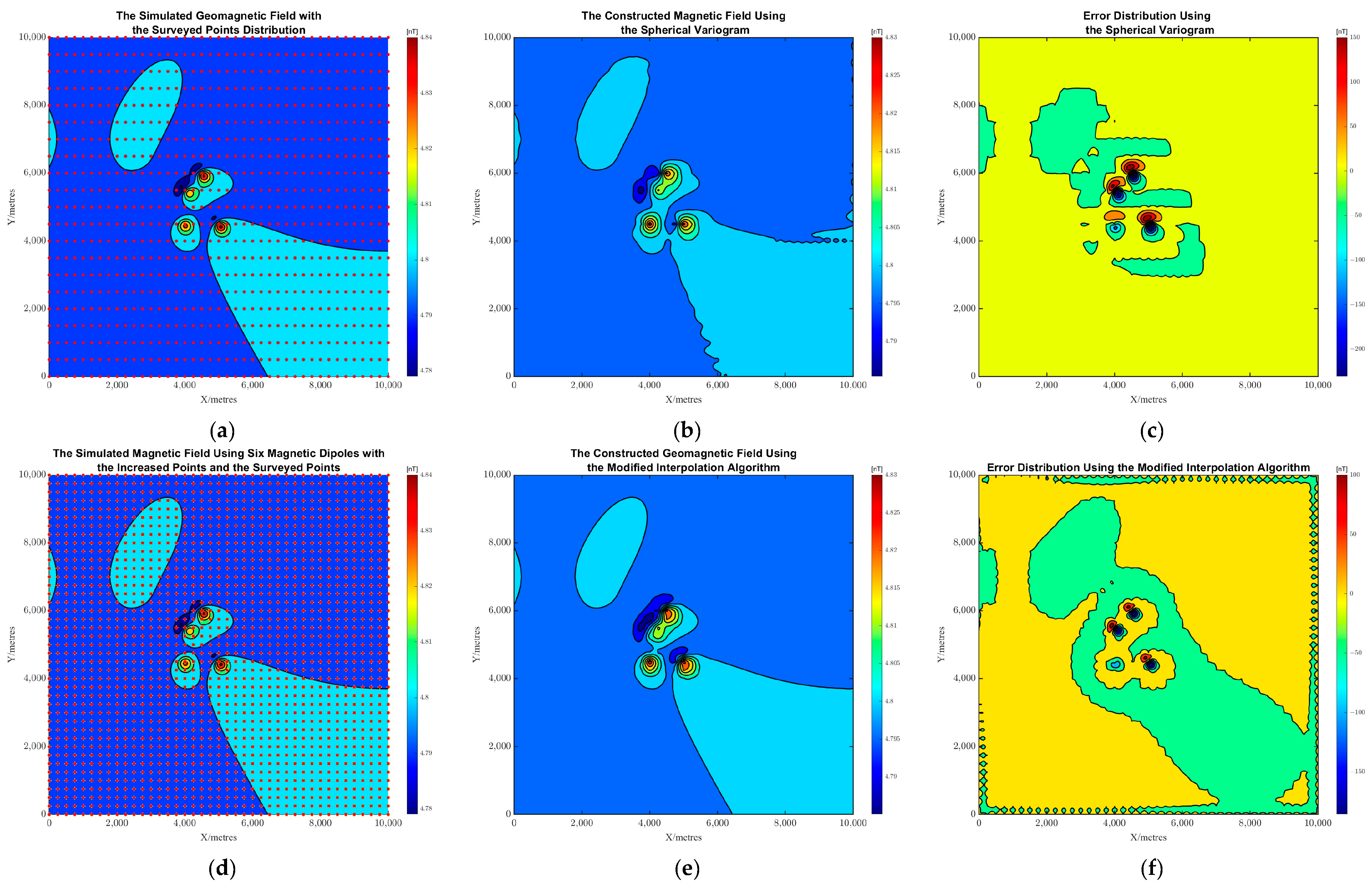
The above simulated geomagnetic map is not representative. Therefore, six magnetic dipoles are used in this paper to simulate the local geomagnetic anomaly region. The relevant parameters are shown in Table 3. The z-axis is specified as the positive direction, the normal field of geomagnetic background is set to 48,000 nT, and the true value of the simulated geomagnetic map with a regional resolution of 50 × 50 m is generated according to the relevant parameters, as shown in Figure 10a. In order to obtain the magnetic samples in the flight-line during the simulation of the aeromagnetic survey, the magnetic data of simulated flight along the Y direction is taken as the measured value on the constructed geomagnetic map, the in-line resolution is set to 250 m, and the flight line spacing is set to 500 m. The schematic diagram of the measurement points is shown in Figure 10b.
Table 3.
Parameters of the six spherical combined model.
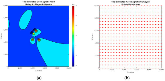
Figure 10.
Diagrams of simulated geomagnetic field with six magnetic dipoles and simulated aeromagnetic measurement points. (a) The simulated geomagnetic map with six magnetic dipoles. (b) Diagram of the simulated aeromagnetic measurement points distribution.
As mentioned above, through data increase processing, the modified algorithm-selected coordinate azimuth angle of 105° is selected for geometric anisotropy processing. The results after processing using the algorithm proposed in this paper are shown in Figure 11e, and the comparison results between the simulation graph and the interpolation graph are shown in Figure 11f. At the same time, this paper uses the traditional spherical variogram to process it, and the results are shown in Figure 11b. The comparison results between the simulation graph and the interpolation graph are shown in Figure 11d. The calculated maximum absolute error (ME), mean absolute error (MAE) and root-mean-square error (RMSE) are shown in Table 4, and the results have been greatly improved.

Figure 11.
A series of diagrams of the simulated geomagnetic map with six magnetic dipoles interpolated by the geometric anisotropy correction algorithm of variogram: (a) diagram of sample data distribution; (b) interpolation map processed by the traditional spherical variogram; (c) comparison results between the simulation map and the interpolation map by the traditional spherical variogram; (d) diagram of increased data distribution; (e) interpolation map processed by the geometric anisotropy correction algorithm of variogram; (f) comparison results between the simulation map and the interpolation map by the geometric anisotropy correction algorithm of variogram.
Table 4.
Comparison of Kriging interpolation errors for the simulated geomagnetic map with six magnetic dipoles using different variogram models.
5. Experiments
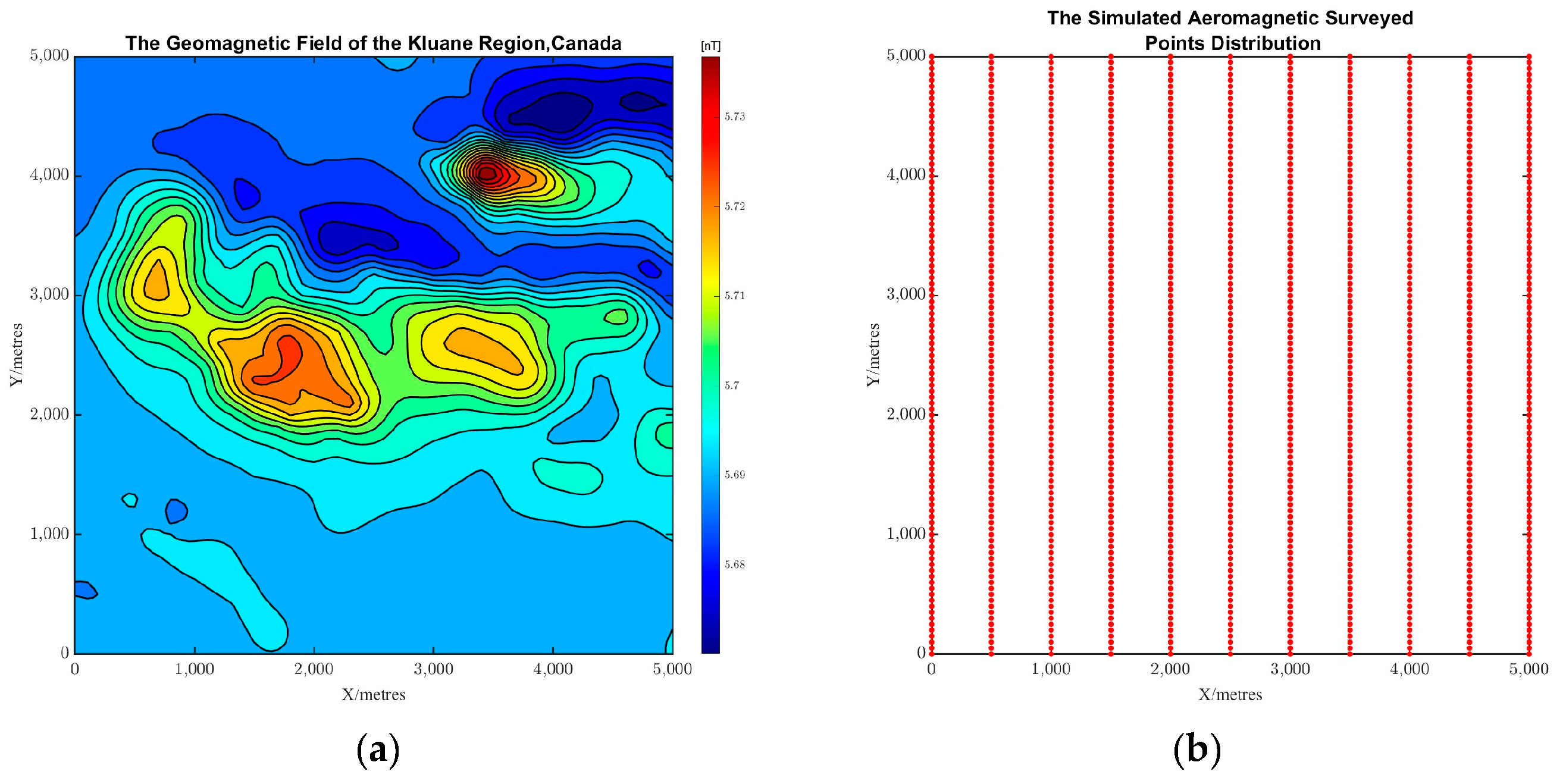
To verify the effectiveness of this method, the aeromagnetic survey data of the Canadian Geological Survey (data sources: Kluane Lake West Aeromagnetic Survey, Residual Total Magnetic Field, NTS 115G/12 and parts of NTS 115G/11, 13, 14 and NTS 115F/9 and 16, Yukon) [18,19] are used for analysis and research. There are abundant deposits and significant magnetic anomalies in the Kluane area. The regional resolution of the geomagnetic map is 50 × 50 m, as shown in Figure 12a.

Figure 12.
The aeromagnetic survey data of the Canadian Geological Survey and the simulated aeromagnetic surveyed points: (a) the geomagnetic map of the Kluane Region, Canada; (b) the simulated aeromagnetic surveyed points.
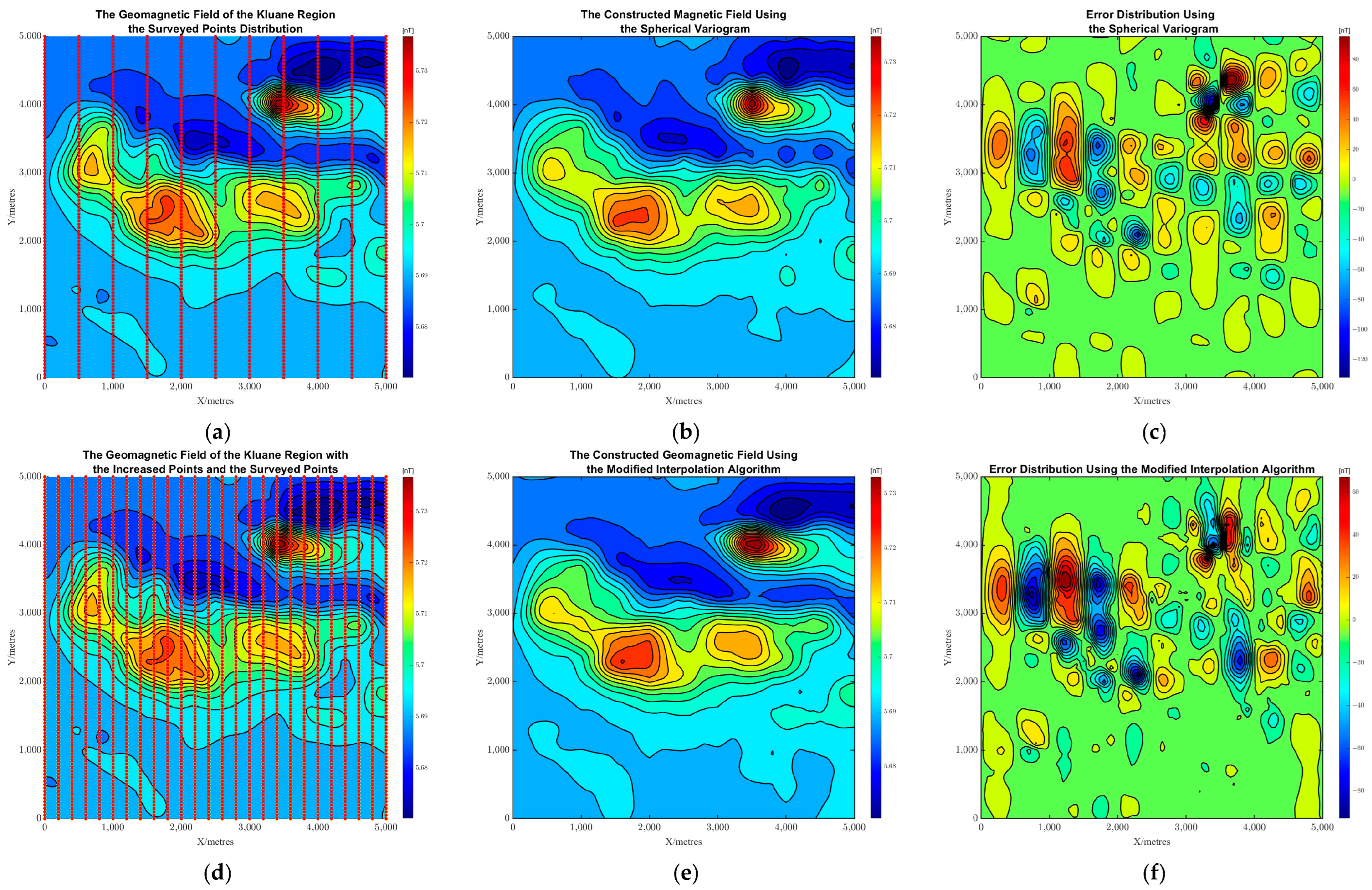
The geomagnetic data with the distance of 500 m in the line-spacing long the Y direction is taken from the geomagnetic map in Figure 12a, and superimposes the Gaussian white noise with a mean of 0 nT and a variance of 0.1, which is taken as the aeromagnetic acquisition data to be interpolated. The spherical model and the method proposed in this paper are respectively used to carry out Kriging interpolation composition. The interpolation results and error distribution are shown in Figure 13b,e. As can be seen from Figure 12, the trend of the geomagnetic map is about 10° downward along the X direction. Through the analysis of the direction–range diagram, the coordinate azimuth angle 162° is selected in this paper for geometric anisotropy processing, and the comparison results between the processed geomagnetic map and the interpolation map are shown in Figure 13e. The 11 lines in Figure 13 are increased according to the algorithm proposed in this paper (as shown in Figure 13d). It can be seen from the comparison chart that the proposed algorithm is better. Meanwhile, compared with the maximum absolute error (ME), mean absolute error (MAE) and root-mean-square error (RMSE) (as shown in Table 5), the calculated results are all improved to a certain extent compared with the results without geometric anisotropy.
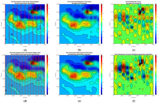
Figure 13.
A series diagrams of geomagnetic interpolation using the geometric anisotropy correction algorithm of variogram: (a) diagram of sample data distribution; (b) interpolation map processed by the traditional spherical variogram; (c) comparison results between the simulation map and the interpolation map by the traditional spherical variogram; (d) diagram of increased data distribution; (e) interpolation map processed by the geometric anisotropy correction algorithm of variogram; (f) comparison of results between the simulation map and the interpolation map by the geometric anisotropy correction algorithm of variogram.
Table 5.
Comparison of Kriging interpolation errors for the aeromagnetic survey data using different variogram models.
6. Conclusions
The main work of this paper includes:
- The influence of geometric anisotropy caused by the sparsity of geomagnetic data on the variability of geomagnetic map construction is analyzed;
- The geometric anisotropy correction formula of the variogram of sparse data is derived;
- A geomagnetic interpolation algorithm based on geometric anisotropy correction of variogram is proposed.
At the same time, through the simulation and measured data test, it is verified that the interpolation accuracy of this method has obvious advantages, which greatly reduces the maximum absolute error, average absolute error and root mean square error, and the performance of ME, MAE and RMSE is improved by at least 10%. Furthermore, the performance is improved by four times in the simulation scene with uncomplicated geomagnetic field based on two magnetic dipoles. To sum up, this modified interpolation algorithm can be applied to the construction of local geomagnetic anomaly maps with high precision and high resolution.
Author Contributions
Conceptualization, M.P. and Q.Z.; methodology, Z.Y., Z.L. and Y.X.; software, H.L., L.Y. and Z.D.; validation, Z.Y. and K.W.; formal analysis, D.C and X.L.; data curation, H.L.; writing—original draft preparation, H.L. and Z.Y.; writing—review and editing, Q.Z. and D.C.; project administration, Q.Z. and W.D.; funding acquisition, Q.Z. All authors have read and agreed to the published version of the manuscript.
Funding
This research was funded by the National Natural Science Foundation of China (No. 12101608).
Data Availability Statement
The data that support the findings of this study are available in Journal of Physics: Conference Series at DOI 10.1088/1742-6596/2486/1/012062, reference 18. These data were derived from the following resources available in the public domain: Kluane Lake West Aeromagnetic Survey, Residual Total magnetic Field, NTS 115G/12 and parts of NTS 115G/11, 13, 14 and NTS 115F/9 and 16, Yukon—Original metadata (https://open.yukon.ca)—Open Government Portal (canada.ca).
Conflicts of Interest
The authors declare no conflicts of interest.
References
- Zhou, W. Aeromagnetic Survey. In Encyclopedia of Engineering Geology; Encyclopedia of Earth Sciences Series; Bobrowsky, P.T., Marker, B., Eds.; Springer: Cham, Switzerland, 2018; pp. 13–18. ISBN 978-3-319-73568-9. [Google Scholar]
- Colin, R. Aeromagnetic Surveys: Principles, Practice and Interpretation|Sebas Sanguil—Academia.Edu. Available online: https://www.academia.edu/16883197/Aeromagnetic_Surveys_Principles_Practice_and_Interpretation (accessed on 10 January 2024).
- Reid, A.B. Aeromagnetic Survey Design. Geophysics 1980, 45, 973–976. [Google Scholar] [CrossRef]
- DB63/T 1933-2021; Technical Specification for Aerial Magnetic Survey of UAV. Administration for Market Regulation of Qinghai Province: Xining, China, 2021. (In Chinese)
- DZ-T-0142-1994; Technical Specification for Airborne Magnetic Survey. Ministry of Land and Resources: Beijing, China, 1994. (In Chinese)
- Xie, X.; Zhao, D.; Liu, C.; Fu, L. Comparative study on different preparation methods of geomagnetic reference map. Eng. Surv. Mapp. 2023, 32, 13–20. (In Chinese) [Google Scholar] [CrossRef]
- Huang, H.; Liu, Q.; Wang, J.; Chen, J.; Yu, X. Kriging-Based Study on the Visualization of Magnetic Method Data. In Proceedings of the 2012 International Conference on Image Analysis and Signal Processing, Hangzhou, China, 9–11 November 2013. [Google Scholar]
- Yang, G.; Zhang, G.; Li, S. Application of universal Kriging interpolation in geomagnetic map. J. Chin. Inert. Technol. 2008, 16, 162–166. (In Chinese) [Google Scholar]
- Cai, C.; Cao, Z.; Zhang, X.; Li, S. A Study for Optimizing the Indoor Geomagnetic Reference Map. J. Geod. Geodyn. 2017, 37, 647–650. (In Chinese) [Google Scholar] [CrossRef]
- Zhao, H.; Zhang, N.; Lin, C.; Lin, P.; Xu, L.; Liu, Y. Construction Method of Geomagnetic Reference Map for Satellite Communication Navigation through Kriging Method. J. Phys. Conf. Ser. 2021, 2033, 012034. [Google Scholar] [CrossRef]
- Wackernagel, H. Multivariate Geostatistics; Springer: Berlin/Heidelberg, Germany, 1995; ISBN 978-3-662-03100-1. [Google Scholar]
- Sun, H. Principle of Geostatistics and Application; China University of Mining and Technology Press: Xuzhou, China, 1990. (In Chinese) [Google Scholar]
- Mcbratney, A.B.; Webster, R. Choosing Functions for Semi-Variograms of Soil Properties and Fitting Them to Sampling Estimates. J. Soil Sci. 1986, 37, 617–639. [Google Scholar] [CrossRef]
- Ai, S.; Ding, X.; Tolle, F.; Wang, Z.; Zhao, X. Latest Geodetic Changes of Austre Lovénbreen and Pedersenbreen, Svalbard. Remote Sens. 2019, 11, 2890. [Google Scholar] [CrossRef]
- Cressie, N.A.C. Statistics for Spatial Data; Wiley series in probability and mathematical statistics; Wiley: New York, NY, USA, 1993; ISBN 978-0-471-00255-0. [Google Scholar]
- Oliver, M.A.; Webster, R. Kriging: A Method of Interpolation for Geographical Information Systems. Int. J. Geogr. Inf. Syst. 1990, 4, 313–332. [Google Scholar] [CrossRef]
- Chen, L.; Cao, J.; Wu, M. Research on Spatial Domain Numerical Methods for Potential Field Continuation in Geomagnetic Navigation; National Defense Industry Press: Arlington, VA, USA, 2015; p. 133. (In Chinese) [Google Scholar]
- Yu, Z.; Pan, M.; Liu, Z. Research on magnetic anomaly detection method assisted by geomagnetic map. J. Phys. Conf. Ser. 2023, 12, 62. [Google Scholar] [CrossRef]
- Open Government Portal|Open Government[EB/OL]. Available online: https://search.open.canada.ca/en/od/ (accessed on 20 March 2023).


Disclaimer/Publisher’s Note: The statements, opinions and data contained in all publications are solely those of the individual author(s) and contributor(s) and not of MDPI and/or the editor(s). MDPI and/or the editor(s) disclaim responsibility for any injury to people or property resulting from any ideas, methods, instructions or products referred to in the content. |
© 2024 by the authors. Licensee MDPI, Basel, Switzerland. This article is an open access article distributed under the terms and conditions of the Creative Commons Attribution (CC BY) license (https://creativecommons.org/licenses/by/4.0/).