Article

Remote Sensing Observations of a Coastal Water Environment Based on Neural Network and Spatiotemporal Fusion Technology: A Case Study of Hangzhou Bay

1
Marine Science and Technology College, Zhejiang Ocean University, Zhoushan 316022, China
2
Shanghai Investigation, Design & Research Institute Co., Ltd., Shanghai 200050, China
3
School of Geography Science and Geomatics Engineering, Suzhou University of Science and Technology, Suzhou 215009, China
4
State Key Laboratory of Estuarine and Coastal Research, East China Normal University, Shanghai 200241, China
*
Author to whom correspondence should be addressed.
Remote Sens. 2024, 16(5), 800; https://doi.org/10.3390/rs16050800
Submission received: 31 December 2023 / Revised: 28 January 2024 / Accepted: 23 February 2024 / Published: 25 February 2024
(This article belongs to the Section Remote Sensing in Geology, Geomorphology and Hydrology)

Abstract

:
The coastal environment is characterized by high, multi-scale dynamics and the corresponding observations from a single remote sensing sensor are still facing challenges in achieving both high temporal and spatial resolution. This study proposed a spatiotemporal fusion model for coastal environments, which could fully enhance the efficiency of remote sensing data use and overcome the shortcomings of traditional spatiotemporal models that are insensitive to small-scale disturbances. The Enhanced Deep Super-Resolution Network (EDSR) was used to reconstruct spatial features in the lower spatial resolution GOCI-II data. The spatial features obtained instead of GOCI-II data were fed into the spatiotemporal fusion model, which enabled the fusion data to achieve an hour-by-hour observation of the water color and morphology information changes at 30 m resolution, including the changes in the spatial and temporal distributions of suspended particulate matter (SPM), the characterization of the vortex street caused by the bridge piers, the inundation process of the tidal flats, and coastline changes. In addition, this study analyzed the various factors affecting fusion accuracy, including spectral difference, errors in both temporal difference and location distance, and the structure of the EDSR model on the fusion accuracy. It is demonstrated that the location distance error and the spectral difference have the most significant impact on the fusion data, which may lead to the introduction of some ambiguous or erroneous spatial features.

1. Introduction

The coastal area has garnered considerable attention due to the frequent impact of human activities. In recent years, the large-scale synchronous observation of coastal information has become achievable with the development of high-resolution spatial and temporal sensors. Earth observation satellites such as GaoFen-1 and Landsat-8/9, with high spatial resolution (<30 m), have been widely utilized for observing small-scale turbidity flows and suspended particulate matter (SPM) in coastal areas [1,2,3]. Geostationary orbit satellites, such as Geostationary Ocean Color Imager (GOCI) and its successor Geostationary Ocean Color Imager: Follow-on (GOCI-II), showcase remarkable temporal resolution with a revisiting period of one hour. Such satellites have found widespread application in the study of tidal current, sediment transport, and harmful algal blooms [4,5,6]. However, constrained by sensor performance, observations of coastal areas using single-source remote sensing data remain at either high temporal or high spatial resolution stages. As a result, there are still a few limitations in observing the water color characteristics and morphological disturbances at small scales over short periods, such as the inundation process of the tidal flats.
Spatiotemporal fusion serves as an effective approach to enhance the efficiency of utilizing remote sensing data and to address the limited temporal or spatial resolution for coastal environment monitoring. Most fusion models, such as the Spatial and Temporal Adaptive Reflectance Fusion Model (STARFM) [7], capture time series changes among high temporal resolution data and apply them to known high spatial resolution data [8]. The enhanced STARFM improves the search method for similar pixels by introducing a conversion coefficient, and this optimization enhances performance, particularly in heterogeneous sites containing numerous mixed pixels [9]. The Flexible Spatiotemporal Data Fusion (FSDAF) model employs an unmixing method to obtain the residuals between high spatial resolution images, which improves the applicability of the model in scenarios of rapid changes in landcover type [10]. Currently, traditional spatiotemporal fusion models have matured and are widely applied in landcover classification, urban flood mapping, and heat island monitoring [11,12,13,14,15,16]. In recent years, with the development of deep learning technology, many studies have explored the application of neural networks in the field of spatiotemporal fusion, which may further enhance the application prospects of spatiotemporal fusion [17]. Song et al. [18] proposed a spatiotemporal fusion framework with Deep Convolutional Neural Networks (STFDCNNs), which employs two convolutional neural networks to learn the complex nonlinear mapping between Landsat and MODIS images. The STFDCNN has been demonstrated to have a satisfactory performance for observing phenological changes. Liu et al. [19] improved the STFDCNN by fully considering the temporal dependence and temporal consistency, and proposed a two-stream convolutional neural network (StfNet) by incorporating temporal information in fine image sequences for spatiotemporal image fusion. Zhang et al. [20] proposed a spatiotemporal fusion method using a generative adversarial network (STFGAN), which is able to learn an end-to-end mapping between the Landsat–MODIS image pairs and predicts a Landsat-like image by considering all the bands, thus significantly improving the accuracy of phenological change and landcover-type change prediction.
In contrast to land applications, there are fewer applications of spatiotemporal fusion technologies focusing on marine and coastal areas. Vanhellemont et al. [21] fused the Spinning Enhanced Visible and InfraRed Imager (SEVIRI) with Moderate Resolution Imaging Spectroradiometer (MODIS) data to observe turbidity in the southern North Sea and English Channel, inheriting SEVIRI’s temporal resolution (15 min) and MODIS’s radiometric resolution, but with a spatial resolution of 3 km, which makes it challenging to meet the observation requirements for coastal areas. Pan et al. [22] fused Landsat-8 with GOCI data, obtaining SPM products at 30 m spatial resolution for the Yangtze Estuary every hour. However, this approach did not effectively address the issue of insensitivity to small-scale land disturbances [23].
In conclusion, the application of spatiotemporal fusion techniques to dynamic coastal observations continues to face challenges, with difficulties arising from the following: (1) Limited remote sensing data. For example, Hangzhou Bay, influenced by irregular semi-diurnal tides, undergoes a tidal cycle every 12 h. As a result, achieving an optimal observation frequency at hourly or even minute-level intervals is crucial. Fusion models like the Enhanced STARFM, STFDCNN, and STFGAN require input from multiple high-resolution data scenes within a tidal cycle, and the limited remote sensing data constrains the application of these models. (2) Complex dynamic changes in coastal regions compared to land. Notably, SPM exhibits significant horizontal and vertical transport, significantly heightening the prediction difficulty. And (3) loss of details after fusion. Some traditional models, due to pixel mixing effects, result in the loss of details in prediction results and exhibit a lower sensitivity in predicting small-scale features, such as fronts, eddies, and changes in submerged areas.
This study employs a neural network model to explore and reconstruct spatial features, significantly enhancing the spatial observation capabilities of low spatial resolution data and addressing the issue of insufficient sensitivity in spatiotemporal fusion models for coastal applications. The fusion method holds the potential to greatly improve the efficiency of remote sensing data utilization. For instance, by integrating Sentinel-2 and Landsat-8/9 data with GOCI-II, it can provide approximately 24 days of high spatiotemporal resolution data (30 m spatial resolution, one scene per hour) annually for the Yangtze Estuary, representing a breakthrough in obtaining high spatiotemporal data where it was previously unavailable. The fusion data contribute to the study of the spatiotemporal distributions of SPM, the characterization of the vortex street caused by the bridge piers, the inundation process of the tidal flats, and coastline changes. Above all, this study provides rich data sources and technical support for environmental monitoring, ecological conservation, site selection for docks, and other studies related to coastal areas.

2. Study Area

The study area is located at Hangzhou Bay (Figure 1), characterized by a strong tidal influence and frequent human activities. The SPM in Hangzhou Bay is influenced by various factors such as runoff, tidal currents, wind waves, and human activities, displaying significant complexity and dynamics. The SPM in Hangzhou Bay consists mainly of south-dispersing Yangtze Estuary sediment after it enters the sea [24]. Its concentration is ultra-high and can reach 1.51 g·L−1 [25], which may be mainly attributed to strong tide- and wave-driven resuspension of bottom sediments and vertically well-mixed masses in the water column [26]. In comparison to natural impacts, human activities often exert more intense and complex influences on the water color and morphological characteristics. For example, bridge construction projects can significantly alter SPM concentrations over several kilometers [27], while deposit-promoting projects swiftly change landcover types [28], affecting nearby erosion–deposition patterns, as well as SPM distribution. Figure 1 shows three regions of interest within Hangzhou Bay, as follows: A.1 was selected to assess the observational capabilities for SPM distributions. This area includes the Hangzhou Bay Bridge and disturbances caused by the bridge piers are a significant focus of engineering considerations. However, rapidly changing disturbance features cannot be effectively observed and analyzed through single-source remote sensing data. A.2 was selected to assess the observational capabilities of the tidal inundation process. This area is a tidal flat located outside the mouth of Hangzhou Bay, covering an area of 20 km2. During the flood tide, high-turbidity water gradually inundates the tidal flat. For low spatial resolution data, accurately delineating the extent of exposed and submerged areas is challenging. A.3 is a muddy tidal flat located on the north bank of Hangzhou Bay, suitable for studying short-to-medium-term coastline changes and changes in landcovers due to sediment transport. Spatiotemporal fusion data increases the observation frequency, making it easier to obtain the land–sea boundary at the same tidal level. This facilitates a quantitative assessment of accumulation and erosion along the coastline.

3. Materials and Methods

3.1. Remote Sensing Data

Landsat-8, launched in February 2013, is a satellite designed to provide seasonal coverage of the global landmass at a spatial resolution of 30 m, allowing for detailed observations of surface features. It passes over Hangzhou Bay at approximately 10:26 local time. The Operational Land Imager (OLI) onboard captures data across five visible–near-infrared (VNIR) bands and two shortwave infrared (SWIR) bands, covering characteristic wavelengths for various surface materials such as aerosols, chlorophyll-a, and SPM. As a successor to Landsat-8, Landsat-9 was launched in September 2021. It carries the enhanced OLI-2 instrument, which benefits from improved radiometric resolution, allowing for a finer detection of radiance changes, particularly suitable for observing darker targets such as water bodies. Orthorectified and terrain-corrected Level 1T products for Landsat-8/9 are available through the United States Geological Survey’s Global Visualization Viewer (GloVis, https://glovis.usgs.gov/, accessed on 1 October 2023), while remote sensing reflectance (Rrs) products can be obtained using ACOLITE software (version 20231023.0) [29,30].
GOCI-II, the successor to the world’s first geostationary water color sensor GOCI, features an improved spatial resolution from 500 m to 250 m. This enhancement enables the capture of more detailed information about spatial changes in coastal areas, providing enhanced monitoring capabilities for SPM distribution, algal bloom dynamics, and shoreline evolution [31]. GOCI-II is equipped with 12 VNIR bands, capturing hourly data from 7:30 to 16:30 local time. Its Level 1B products are provided by the National Institute of Oceanography of Korea (https://www.nosc.go.kr/, accessed on 1 October 2023), and the Rrs products are obtained based on the 6S model [32].

3.2. Radiometric Calibration

Radiometric calibration is the process of converting digital number (DN) values into top-of-atmosphere radiance (LTOA), using gain and offset coefficients, as detailed in Equation (1),
L TOA = gain × DN + offset
The gain and offset values are typically provided by the metadata file in Level 1 products. For Landsat-8/9, the gain and offset differ for each band. In the case of GOCI-II, all bands have a gain of 1e-6 and an offset of 0.

3.3. Atmospheric Correction

The surface reflectance products of Landsat-8/9 are not optimized for turbid water; thus, this study employs the ACOLITE software [29,30] to perform atmospheric correction on Landsat data. The Rayleigh reflectance in the top-of-atmosphere signal can be calculated using the solar and satellite geometric information and the Rayleigh transmittance for each Landsat-8/9 band under a standard atmospheric condition [1,33]. The aerosol reflectance was estimated by Dark Spectrum Fitting (DSF), which calculates aerosol optical thickness (AOT) by utilizing multiple dark targets without a predefined dark band. The look-up table (LUT) employed in DSF was generated using the second simulation of the satellite signal in the solar spectrum-vector (6SV) radiative transfer model [32]. The sun glint reflectance was estimated on SWIR bands and was extrapolated to the VNIR bands using a modeled reflectance shape, as in Harmel et al. [34]. Some studies indicate that the DSF and glint correction works especially well for turbid and productive waters (a water body characterized by high turbidity and high rates of biological productivity), with a minimum root mean square error of 4.6 × 10⁻³ for the water reflectance of Landsat-8 [1,29]. In the Level-2 products generated by ACOLITE software, AOT products are used to assist in the aerosol correction of GOCI-II data, while Rrs products serve as the input for the spatiotemporal fusion model.
Rrs products of GOCI-II provided by the Korea National Ocean Satellite Center exhibit missing data within Hangzhou Bay. Pixels corresponding to extremely turbid waters (e.g., SPM > 1 g·L−1) are identified as clouds or ice, likely contributing to the observed data gaps. As an alternative, the 6SV model was employed for the atmospheric correction of GOCI-II. The 6SV model is a radiative transfer model designed to simulate the interaction of solar radiation with the atmosphere and surface. By inputting the geometric positions of GOCI-II, the solar, atmospheric, and aerosol models’ bands information (spectral response functions or wavelengths), and the surface reflectance characteristics, a relationship between LTOA and surface reflectance can be established. The AOT is provided by Landsat-8/9 products for the given day, with the assumption that AOT remains relatively constant throughout the day. It has been verified that the Rrs of GOCI-II and Landsat-8 has a similar value, with an RMSE less than 0.009 sr−1 (detailed in Section 4.1).

3.4. SPM Inversion

In this study, all obtained SPM concentrations are related to the water quality near the surface, without containing any information about the vertical distribution. The method for estimating SPM concentration is known as the semi-empirical radiative transfer (SERT) model [35,36,37], and its methodology is outlined in Equation (2). Considering that, the Rrs at shorter wavebands is more sensitive to low SPM and at longer wavebands is more sensitive to high SPM [36]. Here, adjustable coefficients α and β are provided for different bands, ensuring sensitivity to SPM changes by switching bands and avoiding saturation issues in shorter wavelength bands. Additionally, to ensure spatial continuity in the inferred SPM distribution from different bands, the maximum SPM concentration value across all bands is utilized [37].
[ SPM ] = 2 × α × R rs β × ( α R rs ) 2
The parameters α and β in Equation (2) are detailed in Table 1, and were calibrated based on the in situ SPM concentration and the spectral response functions of Landsat-8 [22]. While SERT does not comprehensively account for the influence of chlorophyll-a and colored dissolved organic matter, these errors noticeably diminish as the SPM concentration increases. For instance, when the SPM concentration reaches 0.5 g·L−1, such errors will not surpass 10% [22].

3.5. Neural Network and Spatiotemporal Fusion Model

According to the STARFM [7], the predicted pixel values in high spatial resolution data are determined by three primary factors: spectral differences between high and low spatial resolution data, temporal differences among sequences of low spatial resolution observations, and the location distance among the same target. The STARFM assumes that changes in reflectance are consistent and comparable in both high and low spatial resolution images if pixels in low spatial resolution images are pure. In this case, changes derived from coarse pixels can be directly added to pixels in high-resolution images to make predictions. In coastal areas, this ideal condition is often not met. If both clean and mixed coarse pixels coexist, the STARFM can assign higher weights to clean coarse pixels by excluding mixed ones [10]. However, when there are too many mixed coarse pixels, the STARFM may not have enough clean coarse pixels for statistics, leading to a decrease in accuracy.
To enhance the applicability of the STARFM in more complex situations, the Enhanced Deep Super-Resolution Network (EDSR) [38] was employed to reconstruct a coarse pixel into a few purer, fine pixels. The training, validation, and testing datasets for the EDSR model come from Landsat-8/9 imagery over Hangzhou Bay captured on 27 February, 15 March, and 20 December 2022, as well as 29 January 2023. Water bodies within these data were cropped into squares with dimensions of 64 × 64 pixels (approximately 20,000 pieces), out of which, 15,120 pieces were randomly selected as the training dataset, 1680 pieces were selected as the validation dataset, and another 1200 pieces were selected as the testing dataset. The methodology for acquiring true values versus observed values in our dataset is outlined below:
(1)
For all EDSR datasets, the true values correspond to 64 × 64 pixel squares, representing a spatial resolution of 30 m.
(2)
The squares mentioned in (1) are resampled to obtain squares with dimensions of 32 × 32 pixels (60 m spatial resolution) and 16 × 16 pixels (120 m spatial resolution), respectively. These squares serve as transitional data for different upscaling EDSR models and can be used as observed values or true values.
(3)
The squares mentioned in (1) are resampled to obtain squares with dimensions of 8 × 8 pixels (240 m spatial resolution). These squares, with a spatial resolution close to GOCI-II data, serve as observed values for EDSR models.
The EDSR model comprises approximately seven million trainable parameters, and its architectural diagram is depicted in Figure 2. To minimize degradation issues in deep networks [39], only four sets of residual blocks are configured. Each residual block consists of a convolutional activation layer, a convolutional layer, and an addition layer. In the final part of the model, there are 1–3 additional convolutional activation layers, each with an upscaling factor of 2×, aimed at upscaling the data by 21~23 times.
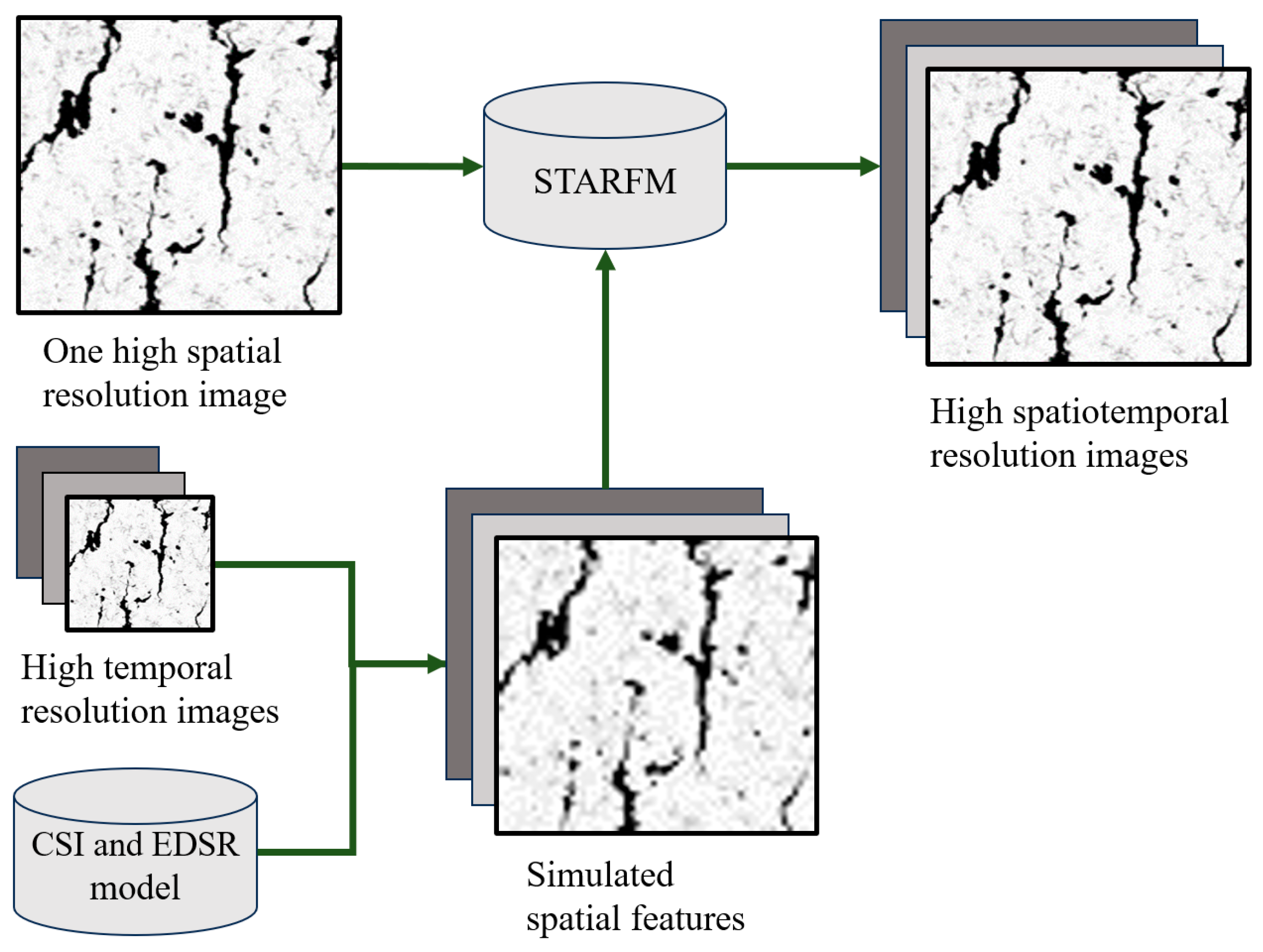
Currently, neural networks like the EDSR model face two challenges in upscaling, as follows: (1) Neural networks exhibit a great feature reconstruction capability when upscaling the data by 2~4 times [40], but encounter issues such as reduced accuracy, excessively large training datasets, and insufficient training parameters when upscaling the data to a higher factor (e.g., 8×). (2) Increasing the depth of neural networks may improve the accuracy and robustness of reconstructions, but it also leads to overfitting, and the spatial features of the data may gradually degrade in excessively deep networks. Section 4.2 provides a detailed evaluation of the feature reconstruction capability of the EDSR model and Cubic Spline Interpolation. The combination of the EDSR model and Cubic Spline Interpolation (CSI) was explored to improve the signal-to-noise ratio and the accuracy of the reconstructions, and the best upscaling model was utilized for the generation of spatiotemporal fusion data. As shown in Figure 3, high temporal resolution images were generated using the upscaling model, producing simulated spatial features with more pure pixels. Therefore, the spatial features obtained from the simulations, rather than the GOCI-II data, were fed into the STARFM. This helps the STARFM learn the pixel relationship corresponding to the high spatial resolution image and the simulated spatial features. At last, this method led to the generation of high spatiotemporal resolution data.

3.6. Assessment Methods

The coefficient of determination (R-squared, R2), Mean Absolute Percentage Error (MAPE), and Root Mean Square Error (RMSE) were employed as metrics to assess the consistency between the actual and predicted values. The equations for these metrics are as follows:
R 2 = [ i = 1 N [ ( y i y i ¯ ) ( x i x i ¯ ) ] i = 1 N ( y i y i ¯ ) 2 i = 1 N ( x i x i ¯ ) 2 ] 2
MAPE = 100 % N i = 1 N x i y i x i
RMSE = 1 N i = 1 N ( x i y i ) 2
In Equations (3)–(5), x represents the actual or high-confidence values, such as the Rrs observed by the GOCI-II; and y represents the predicted or low-confidence values, such as the Rrs observed by Landsat 8/9.
Additionally, Peak Signal-to-Noise Ratio (PSNR) [41] and Structural Similarity (SSIM) [42] are commonly used metrics for assessing the image reconstruction quality, employed here to evaluate the predictive performance of the EDSR model. The PSNR is an error-sensitive image quality assessment metric, reflecting the differences between predicted and actual values, while SSIM is a perceptual model that measures the similarity in brightness, contrast, and structure between predicted and actual values.

4. Results

4.1. Cross-Comparison of Landsat-8/9 and GOCI-II

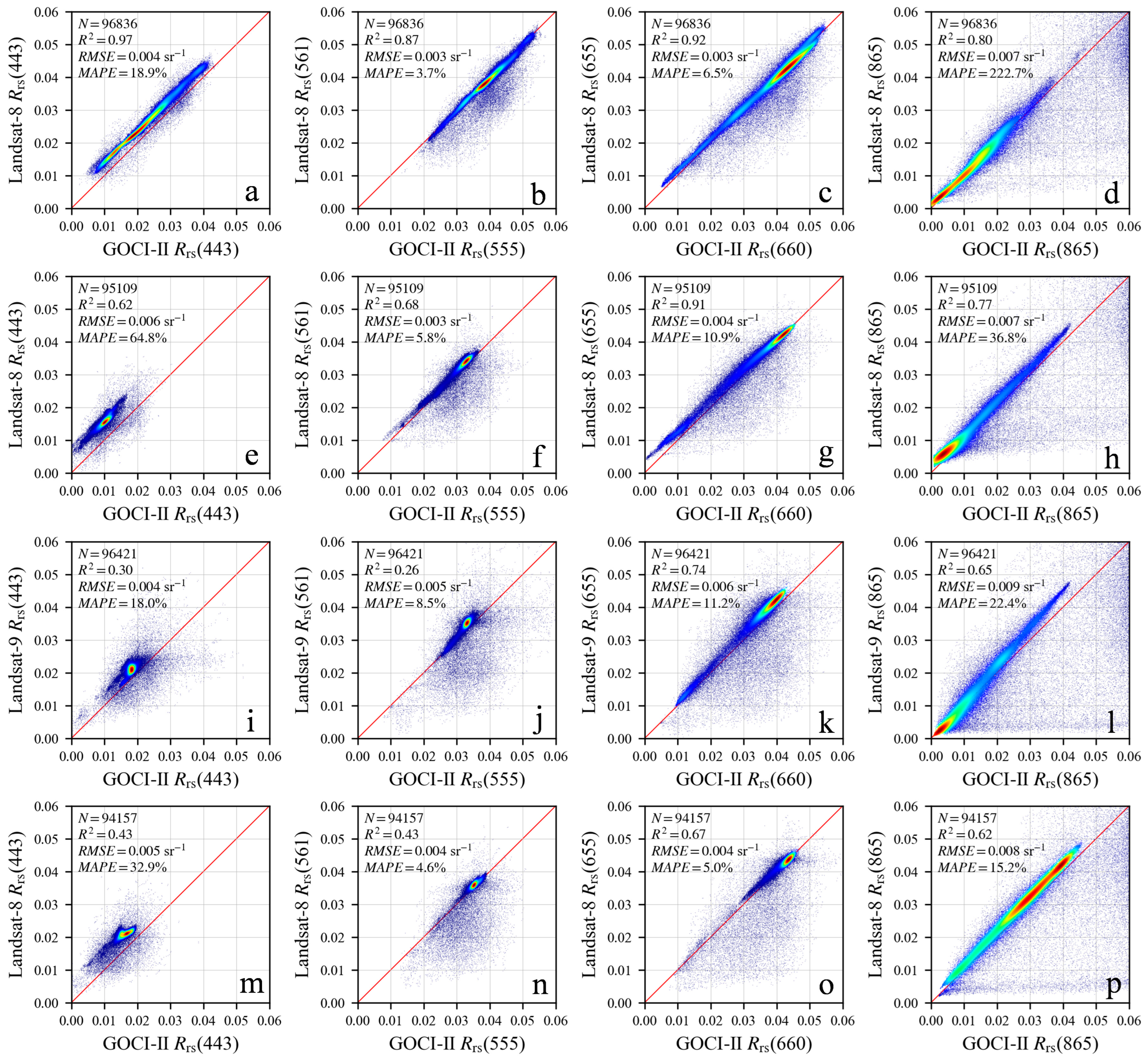
The cross-comparison of the Rrs products from Landsat-8/9 and GOCI-II at a similar moment are shown in Figure 4. The blue bands, being less sensitive to changes in SPM concentration, lead to an unchanged value for both Landsat-8/9 and GOCI-II. In contrast, the red and near-infrared bands show a higher sensitivity to variations in SPM concentration, enabling the inversion of SPM with significant spatial distribution and concentration changes in Hangzhou Bay. The ratio of the Rrs values across all spectral bands between Landsat-8/9 and GOCI-II closely aligns with the 1:1 line, with an RMSE less than 0.009 sr−1. The minimal difference between the satellites may stem from radiometric calibration or atmospheric correction processes, as well as differences in spatial resolution, spectral observation range, and data acquisition time. In summary, the consistent correlations observed in the Rrs from Landsat-8/9 and GOCI-II during four different periods validate the feasibility of utilizing land-based satellites for coastal area observations. This validation is crucial as it establishes the prerequisite for implementing spatiotemporal fusion in coastal areas.

4.2. Evaluation of the Upscaling Model

Currently, the spatial feature reconstruction capability of individual neural network models at a high upscaling factor (e.g., 8×) is yet to be verified. In this section, a quantitative analysis of the spatial feature reconstruction capability of CSI and the EDSR model [38] was conducted. An attempt was made to combine the EDSR model and CSI (e.g., using the EDSR model for upscaling from 240 m to 120 m, and CSI for upscaling from 120 m to 30 m) to obtain a superior upscaling model. The evaluation metrics used include the PSNR and SSIMs.
Figure 5 simulates the feature reconstruction capability of various upscaling models on observed data. Despite some EDSR models having the same network structure and upscaling factor (e.g., [EDSR_240_120] and [EDSR_60_30]), the training process used different observed and real values, resulting in significant differences in the outcomes. The feature reconstruction results in Figure 5b–i show no significant spectral differences compared to the real values. Despite some degradation in spatial representation, small- and medium-scale features such as bridges and islands can still be identified. The PSNR and SSIMs between the predicted values and real values are shown in Table 2.
As shown in Table 2, the feature reconstruction capability of the EDSR model surpasses that of the CSI. Whether using EDSR models directly or combining it with CSI, the reconstruction results consistently outperform CSI in terms of the PSNR, demonstrating the significant potential of EDSR in the spatial reconstruction domain. Compared to the [EDSR_240_30] model, the reconstruction results of the [EDSR_240_120, EDSR_120_30] and [EDSR_240_60, EDSR_60_30] models show a degradation in both the PSNR and SSIMs, which indicates that a single EDSR model is already capable of sufficiently capturing the spatial relationship between observed and true values. Therefore, increasing the trainable parameters may not enhance the feature reconstruction capability of the EDSR model. Among all the upscaling models, the [EDSR_240_120, CSI_120_30] model achieved the best feature reconstruction performance, with a PSNR of 30.29 and SSIM of 0.7845. Therefore, before performing spatiotemporal fusion, feature reconstruction based on the [EDSR_240_120, CSI_120_30] model was applied to GOCI-II data. The obtained spatial features replaced the GOCI-II data as an input for the STARFM model, thereby enhancing the prediction accuracy of spatiotemporal fusion data.

4.3. Example Applications: Spatiotemporal Variation of Coastal Environments

4.3.1. Spatiotemporal Variation of Tidal Flats

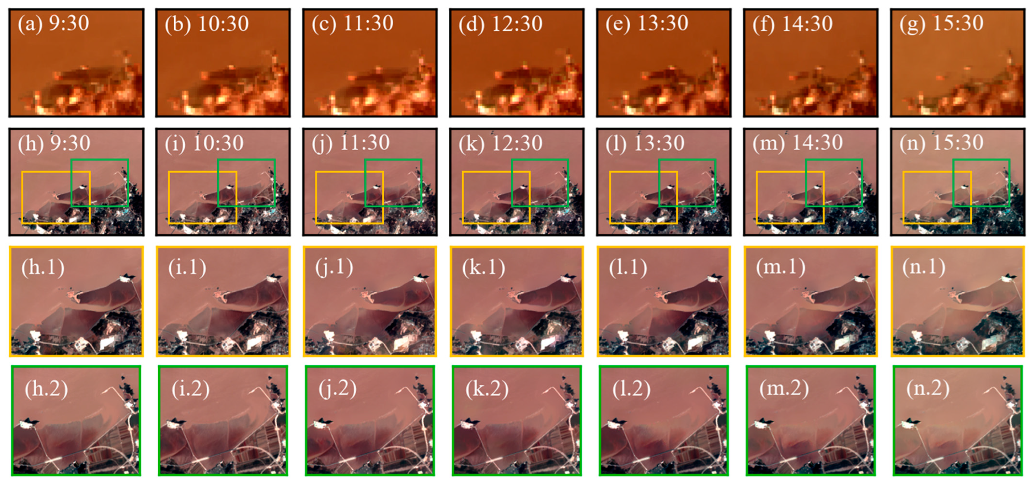
To analyze the observation capabilities of spatiotemporal fusion data for small-scale morphological disturbances, observations were conducted in the coastal area (A.2 in Figure 1). The fusion data were obtained on a day characterized by a neap tide, and the corresponding water level information is detailed in Figure 6. Figure 7 demonstrates the disturbances in the inundation area of two tidal flats under tidal influence. In the true-color images, exposed tidal flats appear as “Chocolate” in color, while high turbidity water appears as “Peru” in color. With the tide rising, both the fusion data and GOCI-II data demonstrate the process of tidal flats gradually being submerged by high turbidity water. Compared to GOCI-II data (Figure 7a–g), the fusion data (Figure 7h–n) not only enables the identification of small-scale features such as tidal channels and embankments, but also provides a more detailed observation of the inundation process of the tidal flats and the extent of exposed and submerged areas. To further illustrate the inundation process, the eastern and western tidal flats are magnified, as indicated by the yellow and green boxes in Figure 7h–n.
During the ebb slack (9:30–11:30), most areas of both the eastern and western tidal flats were exposed, with only the eastern side of the eastern tidal flat being submerged (Figure 7h–j). During the flood tide (12:30–14:30), the eastern tidal flat gradually experienced submersion from east to west by high-turbidity water flow, while the western tidal flat experienced submersion from west to east (Figure 7k–m). At the flood slack (15:30), both the eastern and western tidal flats, along with the tidal channels, were completely submerged by high-turbidity water. Only the eastern side of the western tidal flat had relatively thick sediment, remaining exposed at that time (Figure 7n). Additionally, the Rrs in Figure 7n is higher than in the previous six scenes, resulting in a whitish appearance, which can be attributed to the high solar zenith angle of 69°, causing lower solar irradiance and larger errors in remote sensing observation and fusion results.

4.3.2. Spatiotemporal Variation of SPM Distribution

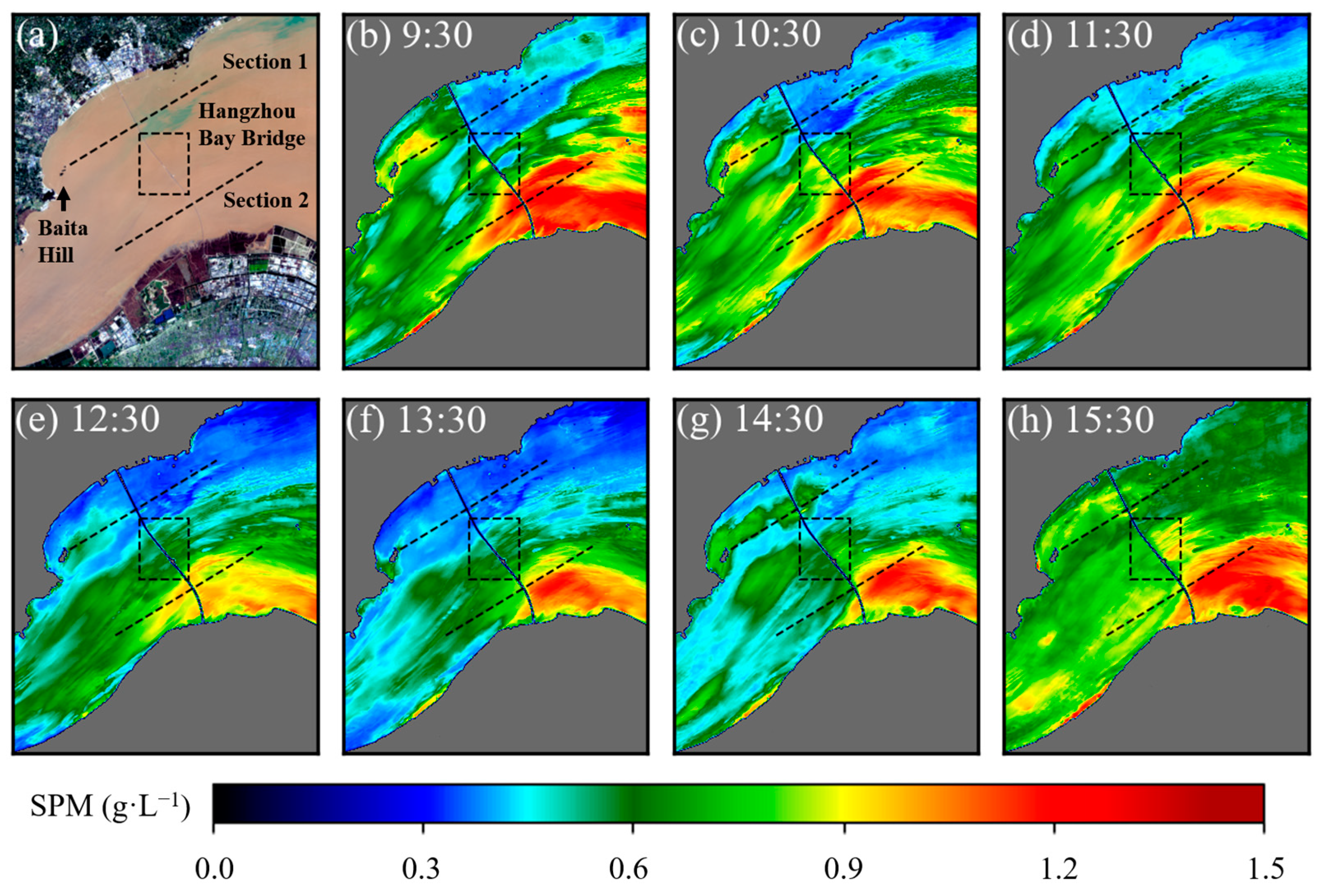
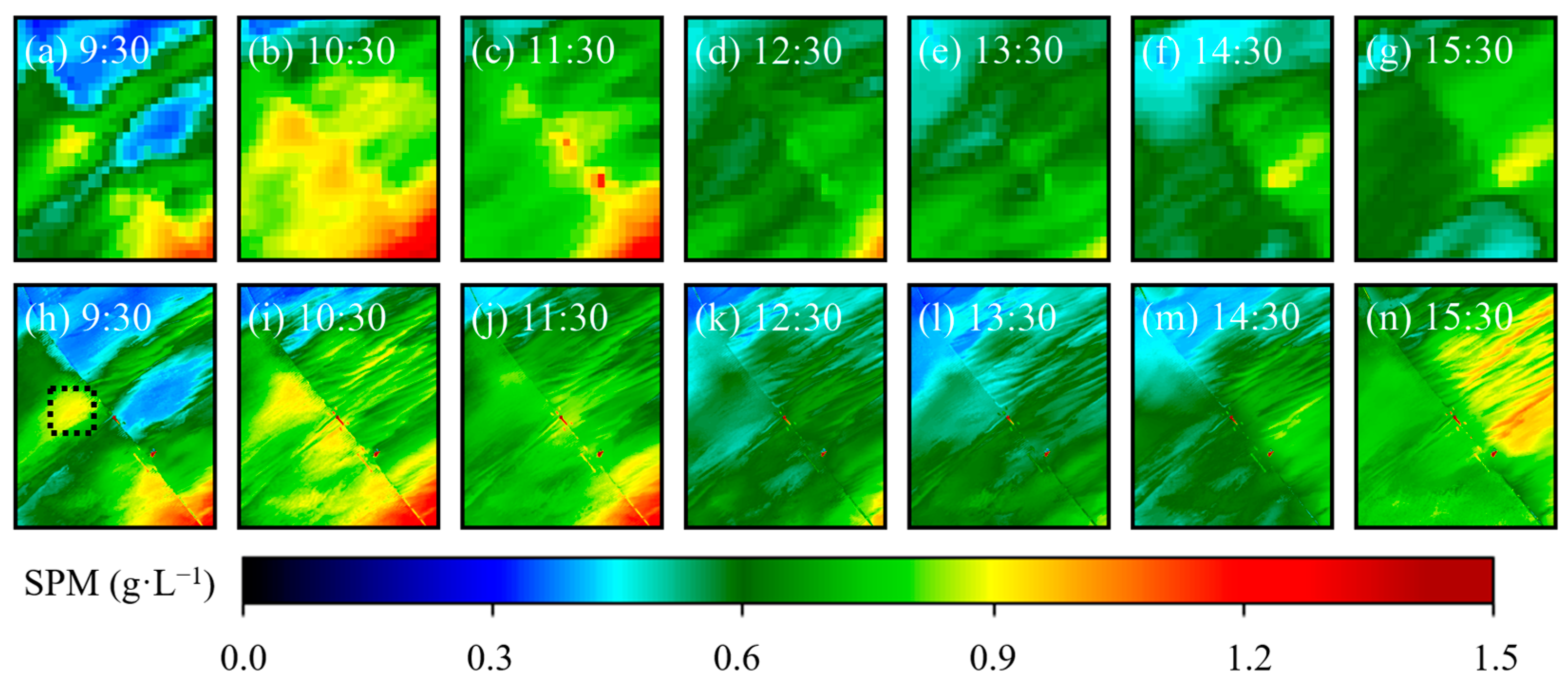
The fusion data offer valuable insights into the highly dynamic distribution of SPM. Figure 8 depicts some medium- and small-scale features in Hangzhou Bay, including the Hangzhou Bay Bridge, areas of high turbidity along the south coast, and the vortex street with high turbidity caused by the bridge piers. To underscore the observational advantages of the fusion data, a region of interest near the Hangzhou Bay Bridge was identified (black dotted box in Figure 8a), showcasing differences in SPM distribution between GOCI-II and fusion data (Figure 9). Additionally, two sections were demarcated along the south and north coasts of Hangzhou Bay (Figure 8a) to monitor the distribution of SPM on the east and west sides of the bridge. This approach allows for a quantitative analysis of the tidal effects on the SPM distribution around water structures such as the bridge piers (Figure 10).
The fusion data were collected on a day characterized by a normal tide, with the corresponding water levels detailed in Figure 10c. During the flood tide (9:30–10:30), the northern part of Hangzhou Bay serves as the main channel for the incoming tide. The rise in water level in this area was significantly faster than that on the southern bank [43]. As the tidal flow passed through bridge piers, it induced a flow separation and generated a high-speed rotating water flow. A horseshoe vortex is generated in front of the bridge piers, while alternating wake vortex streets are generated behind the piers [44,45]. These vortices have a strong sediment-carrying capacity, leading to a rapid increase in the suspended sediment concentration in the surface layer. After passing through the bridge piers from east to west, there was an increase in SPM concentration ranging from 0.12 to 0.25 g/L both at sections 1 and 2, with a notable growth extending up to 2 km. During the flood slack (11:30–12:30), the tidal flow slowed down and the vortex street gradually disappeared. The SPM concentration on the western side of the bridge decreased by around 0.3 g/L, while there was almost no change in SPM concentration on its eastern side. During the ebb tide (13:30–15:30), the southern part of Hangzhou Bay became the main channel for the ebbing flow. After passing through the bridge piers from west to east, the vortex streets, extending 6 to 14 km, formed on their eastern sides, leading to an increase in SPM concentration ranging from 0.25 to 0.35 g/L. Simultaneously, the ebbing flow encountered obstruction from Baita Hill and the bridge piers, resulting in the vortex street extending several kilometers or even tens of kilometers (Figure 8g). According to Figure 10a, the SPM concentration of the vortex street remained around 0.75 g/L. When passing through the bridge piers, the SPM concentration briefly decreased and then rose again to 0.75–0.85 g/L.
The SPM concentration derived from GOCI-II and fusion data exhibit good consistency (Figure 9). Both datasets show similar spatial distribution patterns of SPM changes; high-turbidity water appears in the western area of the bridge during the flood tide (9:30–10:30) and in the eastern area during the ebb tide (14:30–15:30). Due to uneven flow velocities during the flood and ebb tides, the SPM concentration during the flood tide is significantly higher than during the ebb tide. In terms of spatial feature representation, the fusion data (Figure 9h,j–n) and Landsat-8 data (Figure 9i) can both identify the bridge structures. Compared to GOCI-II, the fusion data, accurately displaying abrupt boundaries of SPM, exhibit a greater sensitivity to disturbances in SPM concentration at medium- and small-scales, such as a 2.5 km2 SPM mutation area due to the vortex streets in Figure 9h. However, if the disturbances are too subtle to be detected by GOCI-II observations (such as sediment transitions at the bridge piers or wake turbulence from ships), or if contradictory changes occur simultaneously within a coarse pixel and compensate for each other, the fusion data may not capture effective spatial features in such cases.

4.3.3. Spatiotemporal Variation of Coastline

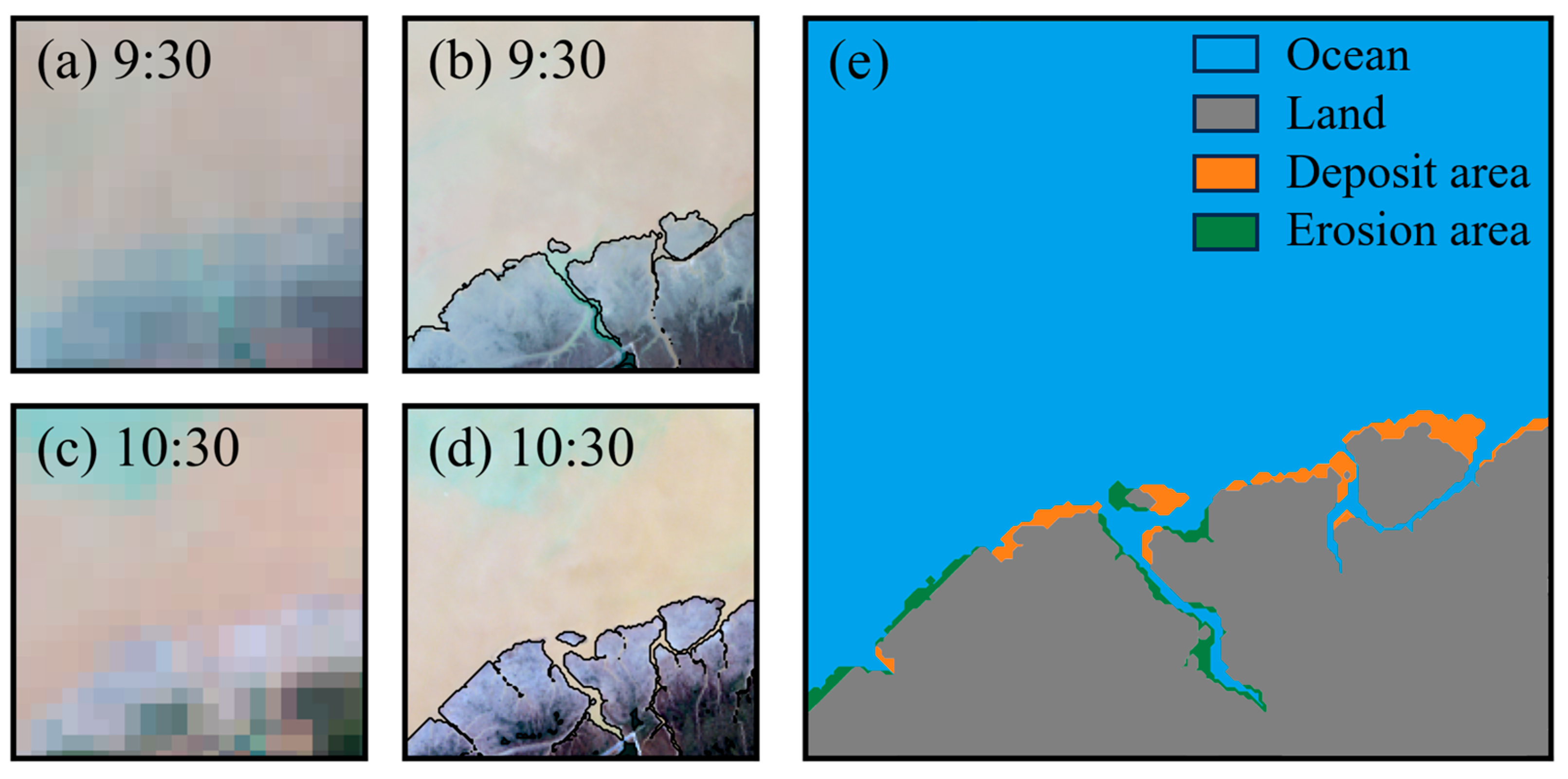
Coastline variation observation based on remote sensing data requires mitigating uncertainties caused by the tidal height, thus imposing strict requirements on the sampling time. Spatiotemporal fusion techniques increase the observation frequency, providing data support for studying coastline and landcover changes in the coastal area over the short- and medium-term. Figure 11 illustrates coastline and landcover changes on the southern coast of Hangzhou Bay (A.3 in Figure 1) between 27 February 2022 and 20 December 2022, using both GOCI-II and fusion data. According to the hydrological information in the Zhapu station (S.1 in Figure 1), both observations occurred during normal tides and at the flood slack, with a water level at 537 cm.
The coastline in the GOCI-II data (Figure 11a,c) appears blurry, making it difficult to distinguish the land and ocean boundaries. In contrast, the fusion data (Figure 11b,d) inherit the spatial features of Landsat-8, enabling the delineation of the boundary between tidal flats and ocean water, based on a simple threshold. The observations in Figure 11e indicate that from February to December, there is approximately 0.4 km2 of deposit area and 0.25 km2 of erosion area along the southern coast of Hangzhou Bay. Due to the lower velocity of the flood tide flow from west to east, sediment deposition occurs on the eastern side of the tidal flats. The flood tide flow is hindered by the tidal flats and gradually slows down, creating favorable conditions for sediment deposition on the eastern side of the tidal flats. In contrast, greater erosion occurs on the western side of the tidal flats, as the higher velocity of the ebb tide flow eroded tidal flats, making the western tidal flats more susceptible to erosion. Additionally, variation in the coastline may also be influenced by sediment transport, waves, and wind forces. Figure 11 indicates that the fusion data from GOCI-II and Landsat-8 increase the likelihood of capturing the land–sea boundary under the same tidal conditions. Moreover, in terms of coastline delineation and accuracy, fusion data provide effective support for studying coastline changes and land area variations.

5. Discussion

5.1. Error Sources and Limitations

The values and accuracy of fusion data are jointly determined by the weights assigned to location distance, temporal difference, and spectral difference. Location distance measures the spatial distance between the central predicted pixel and the surrounding spectral similar candidate pixel. Typically, spatial similarity is better for closer pixels, so a higher weight should be assigned to closer candidates. The error in location distance mainly depends on the geometric calibration accuracy of sensor data. Unfortunately, the uncertainty regarding the geolocation of GOCI-II images remains unclear. As an alternative, this study selected ten point-like land features and, through manual interpretation and statistics, it was found that there is approximately 250 m of geolocation uncertainty between GOCI-II and Landsat-8 images.
Spatial variation in time series data is often emphasized to analyze temporal patterns of landcover changes. The error in temporal difference depends on the accuracy of time series data. Here, according to the signal-to-noise ratio of GOCI-II visible bands, the error in temporal difference is set as 0.14% of the radiance/reflection.
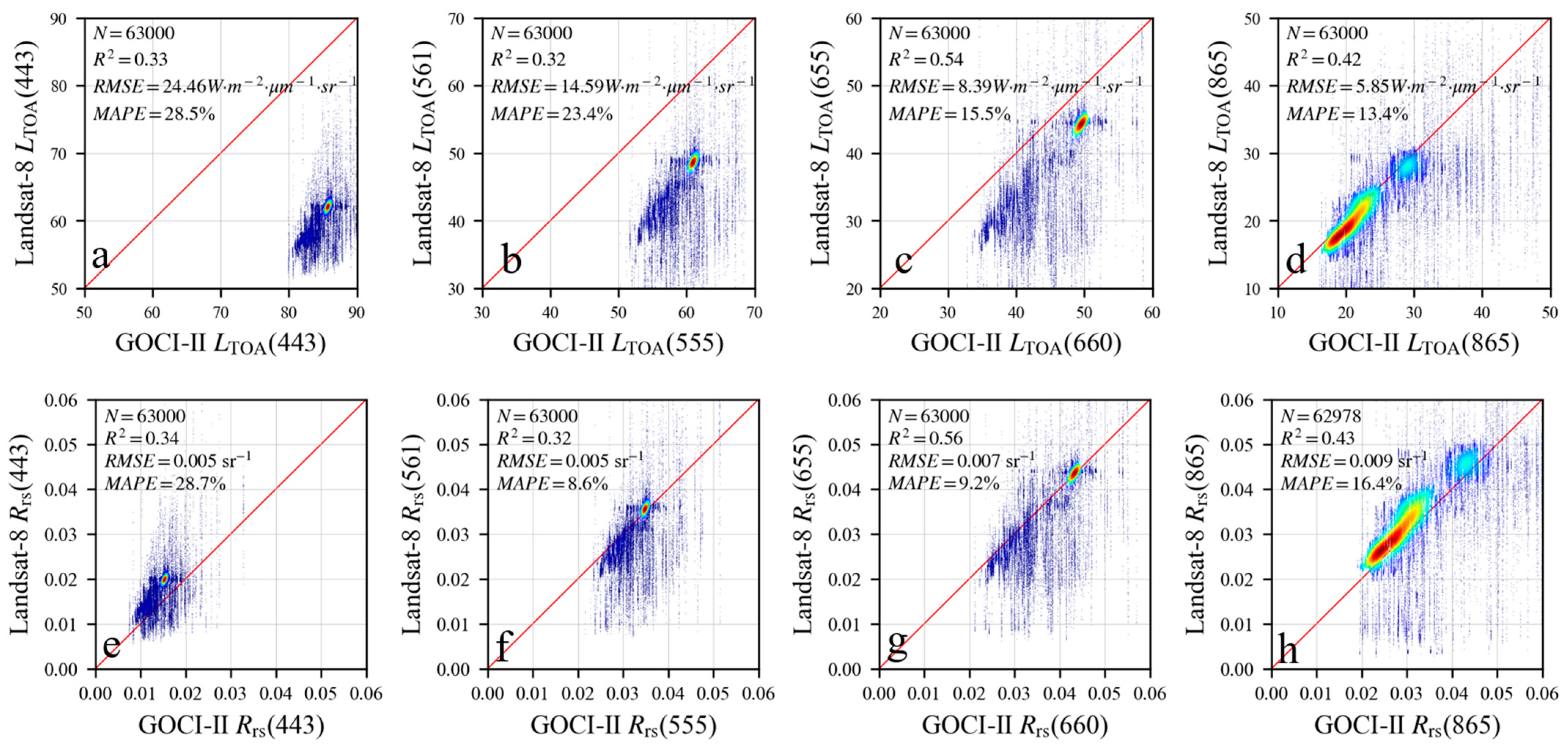
Spectral differences between high and low spatial resolution data within the same period tend to be less noticeable. Some studies assume that errors during preprocessing can be neglected [22], while others utilize simulated data instead of certain remote sensing observations to mitigate these discrepancies [10]. In Section 4.1, a cross-comparison between the Landsat-8/9 and GOCI-II Rrs products yielded consistent results in all VNIR bands. However, if more remote sensing data sources are taken into consideration, the spectral differences between sensor products may become more pronounced. This is particularly critical in coastal waters, where atmospheric correction presents challenges, and variations in SPM are substantial. To quantitatively assess the sources of spectral differences, this study conducted cross-comparisons between the LTOA and Rrs of GOCI-II and Landsat-8, within the A.2 area.
As shown in Figure 12, the overall LTOA of GOCI-II are higher than those of Landsat-8, particularly noticeable in the blue band, where there is an approximate radiance difference of 24 W·m−2·μm−1·sr−1. Conversely, the LTOA in the red and near-infrared bands exhibit better consistency, with differences ranging from 6 to 8 W·m−2·μm−1·sr−1. These differences in LTOA between GOCI-II and Landsat-8 primarily stem from observation angles. GOCI-II has a satellite zenith angle of 36 degrees, much higher than that of Landsat-8 (close to 0 degrees). Consequently, GOCI-II’s LTOA contain more Rayleigh and aerosol scattering signals, especially in the blue band, where higher Rayleigh scattering in the atmosphere results in substantially higher radiance, causing an offset of approximately 20% (Figure 12a–c). Additionally, differences in spectral response functions between the two satellites may contribute to slight radiance variations.
Atmospheric correction eliminates the effects of atmosphere and solar irradiance, extracting the surface signals of water bodies from the LTOA. Consequently, the disparities in Rrs between Landsat-8 and GOCI-II are significantly diminished, with the ratio nearly aligning with the 1:1 line. Minor differences observed in the blue band may stem from spectral response functions or potential atmospheric correction errors. Given the very weak signal of water bodies in this band, an MAPE of 28.7% remains acceptable.
In addition to spectral differences resulting from product processing, another potential contributor to the spectral differences arises from spatial resolution, as depicted by the vertical lines in Figure 12. In Figure 12f,g, the Rrs values of Landsat-8 and GOCI-II show similar mean values. However, there still exists an MAPE of approximately 9%, indicating differences between the mixed coarse pixels in GOCI-II data and the corresponding multiple pure fine pixels in Landsat-8 data.
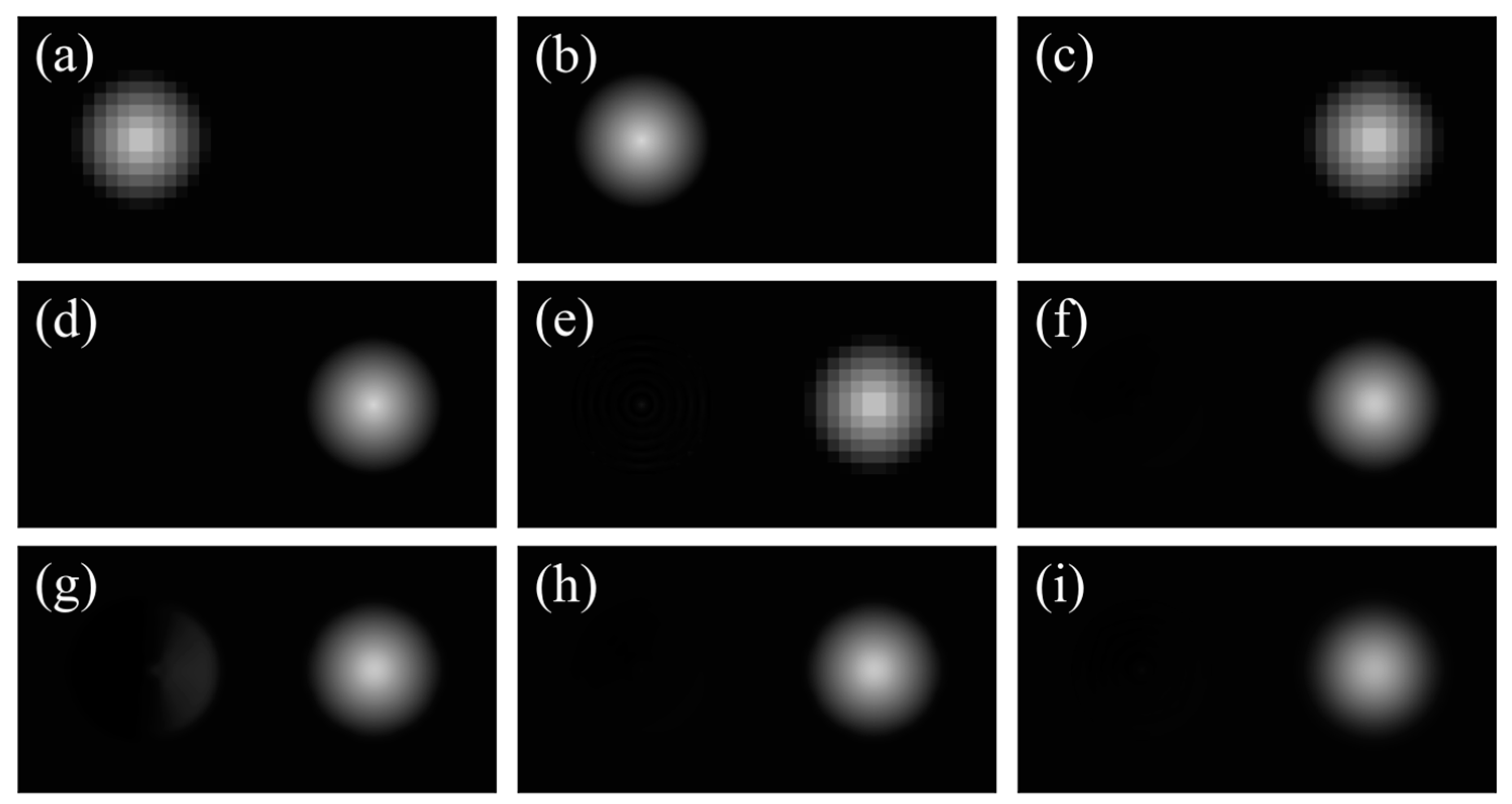
This study quantitatively evaluated the effects of spatial resolution differences, spectral differences, errors in location distance, and temporal differences on fusion processes, using simulated data. The fusion results, along with the data used, are presented in Figure 13. The accuracy of the fusion data obtained under the different models and conditions is shown in Table 3.
Figure 13a,b simulate a pair of high and low spatial resolution data acquired simultaneously, with an 8× difference in spatial resolution. Figure 13c,d display the movement of the sphere (highlighted in bright colors) over time to simulate the horizontal transport of SPM. Figure 13e,f depict the fusion results for Figure 13d based on the information provided in Figure 13a–c. Among all fusion results, Figure 13f,h exhibit the highest accuracy, showing a high similarity to the true value. This indicates that the noise in radiance and reflectance has little impact on the fusion results and can be ignored. Figure 13e demonstrates the degradation caused by spatial resolution differences, which can be effectively mitigated using the EDSR model (as shown in Figure 13f). In Figure 13i, the offset of 20% results in a decrease in SSIMs and the PSNR. Furthermore, upon closer comparison, degradation is primarily concentrated in the peak and valley regions of the images. It can be anticipated that, as the offset value increases, the data quality near the maximum and minimum values of the images will be further degraded. Figure 13g demonstrates the degradation due to location distance errors. These errors lead to the model’s inability to accurately predict the movement of the sphere, resulting in a significant distortion in the start and end positions of the sphere’s movement. Among all factors, the error in location distance and the spectral difference are the primary contributors to fusion errors.
The fusion data based on the LTOA and Rrs are depicted in Figure 14. Fusion data based on LTOA exhibits some erroneous features (Figure 14a–c). On the western side of the tidal flat in Daishan County (Figure 14b), there is a notably “turbid” water outside of the tidal flat (highlighted by the red dashed box). However, such a feature is absent in the corresponding GOCI-II data at the same moment. The possible reason is that the spatiotemporal fusion model erroneously identifies the changes in the tidal flat as changes in the adjacent water area. Similarly, in the eastern side tidal flat (Figure 14c), the features are blurry, making it challenging to determine the extent of the submerged area and water boundaries (red dashed box). This is due to the complex and rapid changes in spectral and spatial features during the inundation process, and the spatiotemporal fusion algorithm fails to correctly identify the changing patterns of these features. In comparison, the features in the fusion data based on Rrs appear clearer (Figure 14d,e). The transformation of LTOA to Rrs does not involve spatial coordinate conversion, resulting in the same location distance error between the Landsat-8 and GOCI-II products. According to the analysis of the simulation (Table 3), the fundamental cause of image distortion in Figure 14b and c lies in radiance differences, or the amplification of location distance errors caused by radiance differences. Additionally, in the true-color images synthesis using the LTOA, the dominance of the blue band as the main component exacerbates the radiance differences, further contributing to the distortion.
Some studies employ georegistration [46,47] and radiometric normalization [47,48] during data preprocessing to reduce the errors mentioned above. In this study, an attempt was made to train high and low spatial resolution data at the corresponding time to eliminate spectral differences between multi-source satellite data. However, the spectral differences are influenced by various factors such as differences in spatial resolution, the accuracy of geometric correction and radiometric calibration, quantization bits (i.e., the sensor’s ability to observe minimum radiance variations), wavelength range signal-to-noise ratio, and satellite geometric location. Such complexity makes it challenging to improve the training accuracy of the EDSR model. At last, the PSNR of the [EDSR_240_30] model is 25.51, and the SSIM is 0.6970, indicating the need for optimizing the network structure or specifying a more reasonable training approach.

5.2. Impact of Network Structure on Feature Reconstruction

According to Lim et al. [38], the EDSR model can increase the number of residual blocks based on the quantization bits of the image, thus achieving better upscaling effects. For images with a higher number of quantization bits (e.g., 8 bits), it is possible to configure 32 residual blocks and place a constant scaling layer at the end of each block, setting the addition factor to 10%, thereby avoiding a decrease in model robustness. In this study, the network structure of the EDSR model with 32 residual blocks was modified (referred to as EDSR* below for distinction from EDSR) and the performance of the EDSR* model was evaluated. The PSNR and SSIMs of the EDSR* models are shown in Table 4.
Compared to EDSR models, EDSR* models exhibit an improved robustness. All the EDSR* models, CSI, and their combined models show similar reconstruction capabilities. Although the residual blocks in the EDSR* models can suppress the decrease in signal-to-noise ratio to some extent, excessively deep networks can still lead to the degradation of spatial features. This leads to a decrease in the PSNR for EDSR* models and, in some cases, a weaker performance than CSI. In contrast, the EDSR models constructed with four convolutional blocks (as detailed in Section 3.5) demonstrate superior feature reconstruction capabilities, with a higher PSNR and SSIMs than EDSR* models.

6. Conclusions

This study proposes a spatiotemporal fusion method for multi-source remote sensing data based on neural networks. The combination of the EDSR model and CSI is utilized to reconstruct spatial features in GOCI-II data and decompose mixed pixels, achieving a SSIM of 0.7845 and a PSNR of 30.29 between the predicted and true values. The reconstructed spatial features, replacing GOCI-II data as the input to the STARFM, address the weakness in sensitivity to disturbances in small-scale features. Leveraging fusion data, this study conducted high spatiotemporal resolution observations of water color and morphological disturbances in Hangzhou Bay. The results indicate that fusion data effectively identifies medium- and small-scale information in coastal areas, such as changes in the inundation area caused by the tidal effects, the vortex street near the bridge piers, hourly variations in SPM distribution, and both short- and medium-term coastline changes. Additionally, this study explores the impact factors on the quality of fusion data, revealing that the error in location distance and the spectral difference are the primary contributors to fusion errors, which can lead to blurring in fusion results and introduce erroneous spatial features.

Author Contributions

Conceptualization, R.T.; Software, R.T.; Methodology, R.T. and F.S; Validation, R.T. and R.J.; Formal analysis, R.T.; Funding acquisition, R.T. and X.W.; Data curation, R.T.; writing—original draft preparation, R.T., X.W. and R.J.; writing—review and editing, X.W., C.C. and F.S. All authors have read and agreed to the published version of the manuscript.

Funding

This research was funded by the “Pioneer” and “Leading Goose” R&D Program of Zhejiang (No.21107000523), the Open Foundation from Marine Sciences in the First-Class Subjects of Zhejiang (No.OFMS001), the Research Project of China Three Gorges Corporation (No.202103552) and Shanghai Investigation, Design & Research Institute Co., Ltd. (No.2022QT(83)-062).

Data Availability Statement

The GOCI-II Level-1 data are available from https://www.nosc.go.kr/eng/program/actionGociDownload.do, accessed on 1 December 2023. The Landsat-8/9 Level-1 data are available from https://glovis.usgs.gov/app, accessed on 1 December 2023. The ACOLITE software can be download from https://github.com/acolite/acolite, accessed on 1 December 2023.

Acknowledgments

We express our gratitude to everyone who helped us to successfully complete this research.

Conflicts of Interest

Author Xiaodao Wei was employed by the Shanghai Investigation, Design & Research Institute Co., Ltd. The remaining authors declare that the research was conducted in the absence of any commercial or financial relationships that could be construed as a potential conflict of interest.

References

  1. Vanhellemont, Q.; Ruddick, K. Turbid wakes associated with offshore wind turbines observed with Landsat 8. Remote Sens. Environ. 2014, 145, 105–115. [Google Scholar] [CrossRef]
  2. Luo, W.; Shen, F.; He, Q.; Cao, F.; Zhao, H.; Li, M. Changes in suspended sediments in the Yangtze River Estuary from 1984 to 2020: Responses to basin and estuarine engineering constructions. Sci. Total Environ. 2022, 805, 150381. [Google Scholar] [CrossRef] [PubMed]
  3. Tian, L.; Wai, O.W.H.; Chen, X.; Li, W.; Li, J.; Li, W.; Zhang, H. Retrieval of total suspended matter concentration from Gaofen-1 Wide Field Imager (WFI) multispectral imagery with the assistance of Terra MODIS in turbid water—Case in Deep Bay. Int. J. Remote Sens. 2016, 37, 3400–3413. [Google Scholar] [CrossRef]
  4. Hu, Z.; Pan, D.; He, X.; Song, D.; Huang, N.; Bai, Y.; Xu, Y.; Wang, X.; Zhang, L.; Gong, F. Assessment of the MCC method to estimate sea surface currents in highly turbid coastal waters from GOCI. Int. J. Remote Sens. 2017, 38, 572–597. [Google Scholar] [CrossRef]
  5. Zhou, Y.; Xuan, J.; Huang, D. Tidal variation of total suspended solids over the Yangtze Bank based on the geostationary ocean color imager. Sci. China Earth Sci. 2020, 63, 1381–1389. [Google Scholar] [CrossRef]
  6. Chen, C.; Liang, J.; Yang, G.; Sun, W. Spatio-temporal distribution of harmful algal blooms and their correlations with marine hydrological elements in offshore areas, China. Ocean Coast. Manag. 2023, 238, 106554. [Google Scholar] [CrossRef]
  7. Gao, F.; Masek, J.G.; Schwaller, M.R.; Hall, F. On the blending of the Landsat and MODIS surface reflectance: Predicting daily Landsat surface reflectance. IEEE Trans. Geosci. Remote Sens. 2006, 44, 2207–2218. [Google Scholar]
  8. Huang, B.; Zhao, Y. Research status and prospect of spatiotemporal fusion of multi-source satellite remote sensing imagery. Acta Geod. Cartogr. Sin. 2017, 46, 1492–1499. [Google Scholar]
  9. Zhu, X.; Chen, J.; Gao, F.; Chen, X.; Masek, J.G. An enhanced spatial and temporal adaptive reflectance fusion model for complex heterogeneous regions. Remote Sens. Environ. 2010, 114, 2610–2623. [Google Scholar] [CrossRef]
  10. Zhu, X.; Helmer, E.H.; Gao, F.; Liu, D.; Chen, J.; Lefsky, M.A. A flexible spatiotemporal method for fusing satellite images with different resolutions. Remote Sens. Environ. 2016, 172, 165–177. [Google Scholar] [CrossRef]
  11. Kim, J.; Hogue, T.S. Evaluation and sensitivity testing of a coupled Landsat-MODIS downscaling method for land surface temperature and vegetation indices in semi-arid regions. J. Appl. Remote Sens. 2012, 6, 63569. [Google Scholar] [CrossRef]
  12. Ouyang, W.; Hao, F.; Skidmore, A.K.; Groen, T.A.; Toxopeus, A.G.; Wang, T. Integration of multi-sensor data to assess grassland dynamics in a Yellow River sub-watershed. Ecol. Indic. 2012, 18, 163–170. [Google Scholar] [CrossRef]
  13. Huang, B.; Wang, J.; Song, H.; Fu, D.; Wong, K. Generating High Spatiotemporal Resolution Land Surface Temperature for Urban Heat Island Monitoring. IEEE Geosci. Remote Sens. Lett. 2013, 10, 1011–1015. [Google Scholar] [CrossRef]
  14. Senf, C.; Leitão, P.J.; Pflugmacher, D.; van der Linden, S.; Hostert, P. Mapping land cover in complex Mediterranean landscapes using Landsat: Improved classification accuracies from integrating multi-seasonal and synthetic imagery. Remote Sens. Environ. 2015, 156, 527–536. [Google Scholar] [CrossRef]
  15. Zhang, F.; Zhu, X.; Liu, D. Blending MODIS and Landsat images for urban flood mapping. Int. J. Remote Sens. 2014, 35, 3237–3253. [Google Scholar] [CrossRef]
  16. Chen, C.; Yang, X.; Jiang, S.; Liu, Z. Mapping and spatiotemporal dynamics of land-use and land-cover change based on the Google Earth Engine cloud platform from Landsat imagery: A case study of Zhoushan Island, China. Heliyon 2023, 9, e19654. [Google Scholar] [CrossRef]
  17. Zhang, Q.; Yuan, Q.; Zeng, C.; Li, X.; Wei, Y. Missing data reconstruction in remote sensing image with a unified spatial–temporal–spectral deep convolutional neural network. IEEE Trans. Geosci. Remote Sens. 2018, 56, 4274–4288. [Google Scholar] [CrossRef]
  18. Song, H.; Liu, Q.; Wang, G.; Hang, R.; Huang, B. Spatiotemporal Satellite Image Fusion Using Deep Convolutional Neural Networks. IEEE J. Sel. Top. Appl. Earth Observ. Remote Sens. 2018, 11, 821–829. [Google Scholar] [CrossRef]
  19. Liu, X.; Deng, C.; Chanussot, J.; Hong, D.; Zhao, B. StfNet: A Two-Stream Convolutional Neural Network for Spatiotemporal Image Fusion. IEEE Trans. Geosci. Remote Sens. 2019, 57, 6552–6564. [Google Scholar] [CrossRef]
  20. Zhang, H.; Song, Y.; Han, C.; Zhang, L. Remote Sensing Image Spatiotemporal Fusion Using a Generative Adversarial Network. IEEE Trans. Geosci. Remote Sens. 2021, 59, 4273–4286. [Google Scholar] [CrossRef]
  21. Vanhellemont, Q.; Neukermans, G.; Ruddick, K. Synergy between polar-orbiting and geostationary sensors: Remote sensing of the ocean at high spatial and high temporal resolution. Remote Sens. Environ. 2014, 146, 49–62. [Google Scholar] [CrossRef]
  22. Pan, Y.; Shen, F.; Wei, X. Fusion of Landsat-8/OLI and GOCI Data for Hourly Mapping of Suspended Particulate Matter at High Spatial Resolution: A Case Study in the Yangtze (Changjiang) Estuary. Remote Sens. 2018, 10, 158. [Google Scholar] [CrossRef]
  23. Hilker, T.; Wulder, M.A.; Coops, N.C.; Linke, J.; McDermid, G.; Masek, J.G.; Gao, F.; White, J.C. A new data fusion model for high spatial-and temporal-resolution mapping of forest disturbance based on Landsat and MODIS. Remote Sens. Environ. 2009, 113, 1613–1627. [Google Scholar] [CrossRef]
  24. Xie, D.; Pan, C.; Wu, X.; Gao, S.; Wang, Z. The variations of sediment transport patterns in the outer Changjiang Estuary and Hangzhou Bay over the last 30 years. J. Geophys. Res. Ocean. 2017, 122, 2999–3020. [Google Scholar] [CrossRef]
  25. Chen, S.L.; Gu, G.C. Modeling suspended sediment concentrations in the mouth of Hangzhou Bay. J. Sediment Res. 2000, 5, 45–50. [Google Scholar]
  26. Xie, D.; Wang, Z.; Gao, S.; De Vriend, H.J. Modeling the tidal channel morphodynamics in a macro-tidal embayment, Hangzhou Bay, China. Cont. Shelf Res. 2009, 29, 1757–1767. [Google Scholar] [CrossRef]
  27. Qiao, S.; Pan, D.; He, X.; Cui, Q. Numerical Study of the Influence of Donghai Bridge on Sediment Transport in the Mouth of Hangzhou Bay. Procedia Environ. Sci. 2011, 10, 408–413. [Google Scholar] [CrossRef]
  28. Shi, Y.; Huang, C.; Shi, S.; Gong, J. Tracking of Land Reclamation Activities Using Landsat Observations—An Example in Shanghai and Hangzhou Bay. Remote Sens. 2022, 14, 464. [Google Scholar] [CrossRef]
  29. Vanhellemont, Q. Adaptation of the dark spectrum fitting atmospheric correction for aquatic applications of the Landsat and Sentinel-2 archives. Remote Sens. Environ. 2019, 225, 175–192. [Google Scholar] [CrossRef]
  30. Vanhellemont, Q.; Ruddick, K. Atmospheric correction of metre-scale optical satellite data for inland and coastal water applications. Remote Sens. Environ. 2018, 216, 586–597. [Google Scholar] [CrossRef]
  31. Ahn, Y.H.; Ryu, J.H.; Cho, S.I.; Kim, S.H. Missions and User Requirements of the 2nd Geostationary Ocean Color Imager (GOCI-II). Korean J. Remote Sens. 2010, 26, 277–285. [Google Scholar]
  32. Vermote, E.F.; Tanré, D.; Deuze, J.L.; Herman, M.; Morcette, J. Second Simulation of the Satellite Signal in the Solar Spectrum, 6S: An overview. IEEE Trans. Geosci. Remote Sens. 1997, 35, 675–686. [Google Scholar] [CrossRef]
  33. Gordon, H.R.; Brown, J.W.; Evans, R.H. Exact Rayleigh scattering calculations for use with the Nimbus-7 Coastal Zone Color Scanner. Appl. Opt. 1988, 27, 862–871. [Google Scholar] [CrossRef] [PubMed]
  34. Harmel, T.; Chami, M.; Tormos, T.; Reynaud, N.; Danis, P. Sunglint correction of the Multi-Spectral Instrument (MSI)-SENTINEL-2 imagery over inland and sea waters from SWIR bands. Remote Sens. Environ. 2018, 204, 308–321. [Google Scholar] [CrossRef]
  35. Shen, F.; Zhou, Y.; Li, J.; He, Q.; Verhoef, W. Remotely sensed variability of the suspended sediment concentration and its response to decreased river discharge in the Yangtze estuary and adjacent coast. Cont. Shelf Res. 2013, 69, 52–61. [Google Scholar] [CrossRef]
  36. Shen, F.; Verhoef, W.; Zhou, Y.; Salama, M.S.; Liu, X. Satellite Estimates of Wide-Range Suspended Sediment Concentrations in Changjiang (Yangtze) Estuary Using MERIS Data. Estuaries Coasts 2010, 33, 1420–1429. [Google Scholar] [CrossRef]
  37. Shen, F.; Zhou, Y.; Peng, X.; Chen, Y. Satellite multi-sensor mapping of suspended particulate matter in turbid estuarine and coastal ocean, China. Int. J. Remote Sens. 2014, 35, 4173–4192. [Google Scholar] [CrossRef]
  38. Lim, B.; Son, S.; Kim, H.; Nah, S.; Lee, K.M. Enhanced Deep Residual Networks for Single Image Super-Resolution. In Proceedings of the 2017 IEEE Conference on Computer Vision and Pattern Recognition Workshops (CVPRW), Honolulu, HI, USA, 21–26 July 2017; pp. 1132–1140. [Google Scholar]
  39. He, K.; Zhang, X.; Ren, S.; Sun, J. Deep Residual Learning for Image Recognition. In Proceedings of the Conference on Computer Vision and Pattern Recognition, Las Vegas, NV, USA, 27–30 June 2016; pp. 770–778. [Google Scholar]
  40. Dong, C.; Loy, C.C.; Tang, X. Accelerating the Super-Resolution Convolutional Neural Network. In Proceedings of the Computer Vision–ECCV 2016: 14th European Conference, Amsterdam, The Netherlands, 11–14 October 2016; Springer: Berlin/Heidelberg, Germany, 2016. Part II 14. pp. 391–407. [Google Scholar]
  41. Wang, Z.; Bovik, A.C.; Sheikh, H.R.; Simoncelli, E.P. Image quality assessment: From error visibility to structural similarity. IEEE Trans. Image Process 2004, 13, 600–612. [Google Scholar] [CrossRef]
  42. Horé, A.; Ziou, D. Image Quality Metrics: PSNR vs. SSIM. In Proceedings of the 2010 20th International Conference on Pattern Recognition, Istanbul, Turkey, 23–26 August 2010; pp. 2366–2369. [Google Scholar]
  43. Liu, M.; Shen, F.; Ge, J.Z.; Kong, Y.Z. Diurnal variation of suspended sediment concentration in Hangzhou Bay from geostationary satellite observation and its hydrodynamic analysis. J. Sediment Res. 2013, 1, 7–13. [Google Scholar]
  44. Skrbek, L.; Vinen, W.F. The Use of Vibrating Structures in the Study of Quantum Turbulence. In Progress in Low Temperature Physics; Elsevier: Amsterdam, The Netherlands, 2009; Volume 16, pp. 195–246. [Google Scholar]
  45. Ahmad, N.; Kamath, A.; Bihs, H. 3D numerical modelling of scour around a jacket structure with dynamic free surface capturing. Ocean Eng. 2020, 200, 107104. [Google Scholar] [CrossRef]
  46. Emelyanova, I.V.; McVicar, T.R.; Van Niel, T.G.; Li, L.T.; Van Dijk, A.I. Assessing the accuracy of blending Landsat–MODIS surface reflectances in two landscapes with contrasting spatial and temporal dynamics: A framework for algorithm selection. Remote Sens. Environ. 2013, 133, 193–209. [Google Scholar] [CrossRef]
  47. Gevaert, C.M.; García-Haro, F.J. A comparison of STARFM and an unmixing-based algorithm for Landsat and MODIS data fusion. Remote Sens. Environ. 2015, 156, 34–44. [Google Scholar] [CrossRef]
  48. Gao, F.; Masek, J.G.; Wolfe, R.E.; Huang, C. Building a consistent medium resolution satellite data set using moderate resolution imaging spectroradiometer products as reference. J. Appl. Remote Sens. 2010, 4, 43526. [Google Scholar]
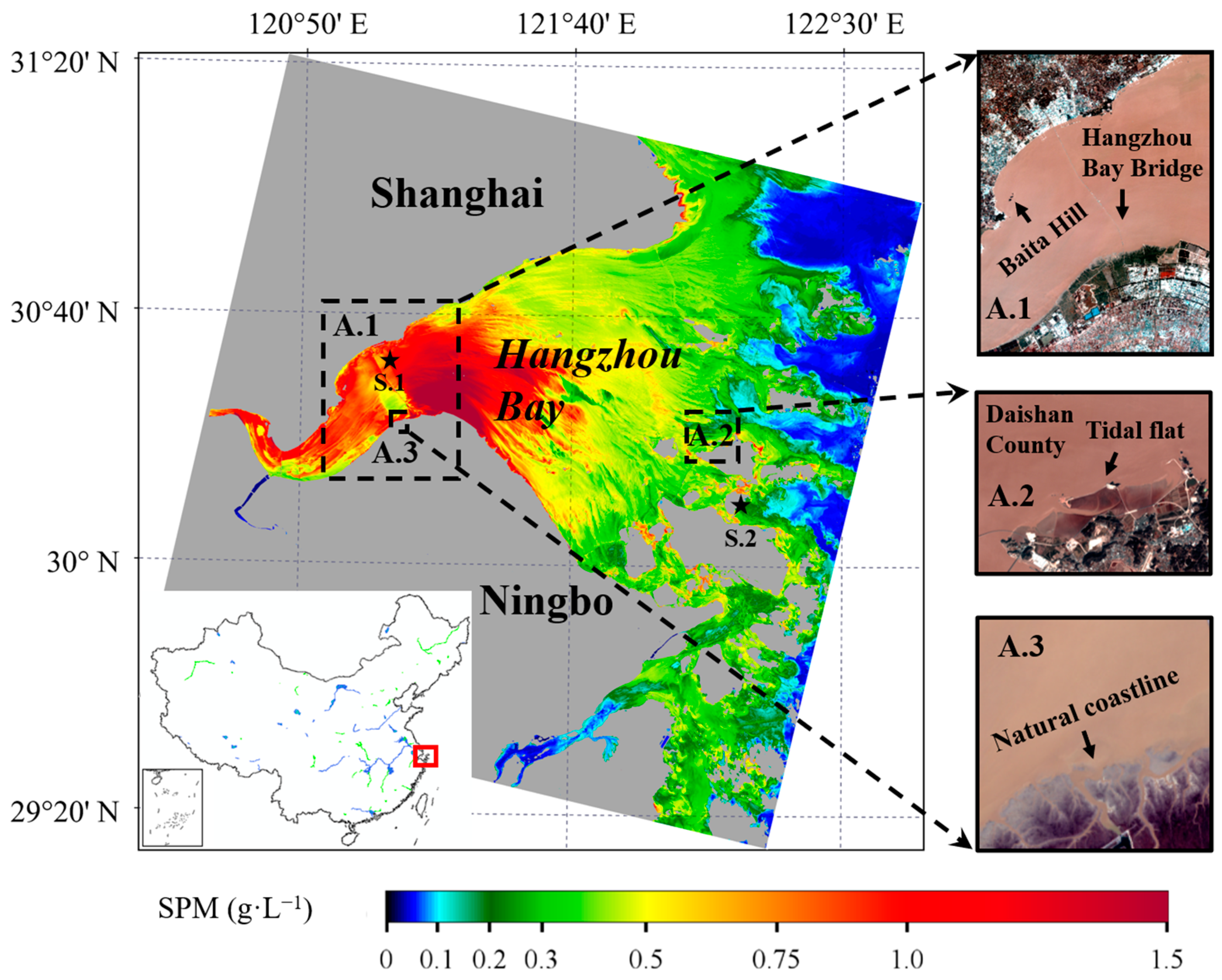
Figure 1. The study area and the SPM distribution based on Landsat-9 data on 20 December 2022. A.1, A.2, and A.3 are the regions of interest for water color and morphological dynamics observations. The star (★) signifies the locations of the Zhapu (S.1) and Daishan (S.2) hydrological stations, which supplied measured water levels for the regions of interest.
Remotesensing 16 00800 g001
Figure 2. Structure of the EDSR model.
Remotesensing 16 00800 g002
Figure 3. The production process of high spatiotemporal fusion data.
Remotesensing 16 00800 g003
Figure 4. Cross-comparison of Rrs in the blue, green, red, and near-infrared bands of GOCI-II and Landsat 8/9. From top to bottom, each row corresponds to the comparison results on 27 February 2022 (ad), 15 March 2022 (eh), 20 December 2022 (il), and 29 January 2023 (mp).
Remotesensing 16 00800 g004
Figure 5. The feature reconstruction capability of multiple upscaling models on observed data. (a) Observations of the model with a spatial resolution of 240 m; (bi) high spatial resolution data, predicted based on the EDSR model, CSI, and their combination models, with a target spatial resolution of 30 m. The model is named in the format of [upscaling method_origin spatial resolution_target spatial resolution]. For example, [EDSR_240_120, CSI_120_30] refers to the model trained by EDSR, which reconstructs 240 m spatial resolution data into 120 m spatial resolution data, and then upscales it to 30 m using CSI; (j) the true values of the data, with a spatial resolution of 30 m, were used to evaluate the feature reconstruction effects of the models.
Remotesensing 16 00800 g005
Figure 6. Water levels at Daishan Hydrological Station obtained from the Global Tide Prediction Service Platform (http://global-tide.nmdis.org.cn/, accessed on 1 October 2023), hollow circles are hourly predicted water levels, and the gray columns correspond to the observation periods of GOCI-II and fusion data in Figure 7.
Remotesensing 16 00800 g006
Figure 7. True-color observations of GOCI-II, Landsat-8, and fusion data on the north shore tidal flats of Daishan County on 29 January 2023, from 9:30 to 15:30. (ag) Disturbances in the inundation area of the east–west tidal flats observed by GOCI-II; (h,jn) predicted results of spatiotemporal fusion at the corresponding moments of GOCI-II; (i) observation data of Landsat-8; (h.1n.1) spatiotemporal variations of the western tidal flats, corresponding to the yellow box in (hn); (h.2n.2) spatiotemporal variations of the eastern tidal flats, corresponding to the green box in (hn).
Remotesensing 16 00800 g007
Figure 8. Spatial distribution of SPM in the central part of Hangzhou Bay on 15 March 2022. (a) Landsat-8 true-color composite image with two sections and a region of interest detailed in Figure 9 and Figure 10; (bh) variation of the spatial distribution of SPM in central Hangzhou Bay derived from fusion data.
Remotesensing 16 00800 g008
Figure 9. Spatial distribution of SPM concentrations near Hangzhou Bay Bridge from GOCI-II and fusion data inversion. (ag) SPM concentrations derived from GOCI-II data near Hangzhou Bay Bridge on 15 March 2022, 9:30–15:30; (h,jn) SPM concentration derived from spatiotemporal fusion data near Hangzhou Bay Bridge, the black dotted box in (h) represents the SPM mutation area near the bridge pier due to vortex streets; (i) SPM concentrations derived from Landsat-8 data near Hangzhou Bay Bridge on 15 March 2022, 10:30.
Remotesensing 16 00800 g009
Figure 10. SPM distribution on March 15 2022 at the north and south cross-sections of the Hangzhou Bay Bridge. (a) SPM distribution at Section 1 in the northern part of the Hangzhou Bay Bridge from 9:30 to 15:30. A data gap at 10 km was caused by the bridge cover-up; (b) SPM distribution at Section 2 in the southern part of the Hangzhou Bay Bridge from 9:30 to 15:30; (c) water level at Zhapu station (S.1 in Figure 1), hollow circles are predicted tide heights and gray columns are the observation periods of the GOCI-II.
Remotesensing 16 00800 g010
Figure 11. Spatiotemporal variation in the coastline on the southern coast of Hangzhou Bay observed by GOCI-II and fusion data. (a,b) GOCI-II and fusion data observation at 9:30 on 27 February 2022; (c,d) GOCI-II and fusion data observation at 10:30 on 20 December 2022. (e) Coastal deposit (orange) and erosion (green) areas identified by fusion data.
Remotesensing 16 00800 g011
Figure 12. Cross-comparison between GOCI-II and Landsat-8 on 29 January 2023, in the A.2 area (the tidal flats in Figure 1). Warmer colors represent areas with higher point density, while cooler colors indicate lower density regions. (ad) scatter plot of the LTOA; (eh) scatter plot of the Rrs.
Remotesensing 16 00800 g012
Figure 13. Model performance evaluation and error analysis based on simulated data. (a) Low spatial resolution image at time t1; (b) high spatial resolution image at time t1; (c) low spatial resolution image at time t2; (d) high spatial resolution image at time t2, serving as the true value for the fusion data; (e) fusion data predicted based on the STARFM; (f) fusion data predicted based on the EDSR model and the STARFM under theoretical conditions; (g) fusion data predicted based on the EDSR model and the STARFM considering location distance error (250m); (h) fusion data predicted based on the EDSR model and the STARFM considering temporal difference error (0.14% random noise); (i) fusion data predicted based on the EDSR model and the STARFM considering a spectral difference with a 20% offset added to the low spatial resolution image.
Remotesensing 16 00800 g013
Figure 14. True-color fusion data of the tidal flats along the northern side of Daishan County at 14:30 on 29 January 2023. (a) Spatiotemporal fusion data generated by LTOA of GOCI-II and Landsat-8; (b,c) western and eastern tidal flats in the fused data, incorrect spatial features are marked by red boxes; (d,e) corresponding fusion data of (b,c) generated using the Rrs.
Remotesensing 16 00800 g014
Table 1. SERT model parameters corresponding to the Landsat 8/9 bands, used for SPM inversion of fused data.
Bands (nm)αβ
5610.050932.2256
6550.076211.5345
8650.10381.8042
Table 2. Feature reconstruction capacity assessment of the EDSR model, CSI, and their combined models.
ModelsPSNRSSIM
CSI_240_3029.490.7797
CSI_240_60, EDSR_60_3029.830.7806
CSI_240_120, EDSR_120_3030.060.7814
EDSR_240_120, CSI_120_3030.290.7845
EDSR_240_60, CSI_60_3030.110.7779
EDSR_240_3030.120.7831
EDSR_240_120, EDSR_120_3030.110.7788
EDSR_240_60, EDSR_60_3029.970.7783
Table 3. The R2, MAPE, PSNR, and SSIM of the fusion data obtained under different models and conditions.
Fusion Data in Figure 13R2MAPEPSNRSSIM
(e)0.98348.1%42.350.9415
(f)0.99820.1%51.880.9793
(g)0.93051.95%35.840.8529
(h)0.99819.55%51.860.9790
(i)0.99421.96%43.980.9646
Table 4. Feature reconstruction capacity assessment of the EDSR* model, CSI, and their combined models.
ModelsPSNRSSIM
CSI_240_3029.490.7797
CSI_240_60, EDSR*_60_3029.480.7786
CSI_240_120, EDSR*_120_3029.410.7756
EDSR*_240_120, CSI_120_3028.990.7733
EDSR*_240_60, CSI_60_3029.400.7732
EDSR*_240_3029.800.7784
EDSR*_240_120, EDSR*_120_3028.990.7704
EDSR*_240_60, EDSR*_60_3029.500.7786
Disclaimer/Publisher’s Note: The statements, opinions and data contained in all publications are solely those of the individual author(s) and contributor(s) and not of MDPI and/or the editor(s). MDPI and/or the editor(s) disclaim responsibility for any injury to people or property resulting from any ideas, methods, instructions or products referred to in the content.