Abstract
The three-dimensional (3D) reconstruction of buildings using photogrammetric point clouds is important for many applications, ranging from digital city construction to urban energy consumption analysis. However, problems such as building complexity and point cloud flaws may lead to incorrect modeling, which will affect subsequent steps such as texture mapping. This paper introduces a pipeline for building surface reconstruction from photogrammetric point clouds, employing a hybrid method that combines connection evaluation and framework optimization. Firstly, the plane segmentation method divides building point clouds into several pieces, which is complemented by a proposed candidate plane generation method aimed at removing redundancies and merging similarities. Secondly, the improved connection evaluation method detects potential skeleton lines from different planes. Subsequently, a framework optimization method is introduced to select suitable undirected polygonal boundaries from planes, forming the basis for plane primitives. Finally, by triangulating all plane primitives and filling holes, a building surface polygonal model is generated. Experiments conducted on various building examples provide both qualitative and quantitative evidence that the proposed hybrid method outperforms many existing methods, including traditional methods and deep learning methods. Notably, the proposed method successfully reconstructs the main building structures and intricate details, which can be further used to generate textural models and semantic models. Experimental results validate that the proposed method can be used for the surface reconstruction from photogrammetric point clouds of planar buildings.
1. Introduction
Recently, 3D digital city modeling using aerial images is a popular research field. Aerial images can provide not only geometric position information but also texture information, which can satisfy the whole reconstruction process of generating photogrammetric point clouds, surface model modeling and texture mapping. It is worth emphasizing that buildings constitute a pivotal element of the urban landscape, and their modeling has a substantial impact [1]. Through entities in conjunction with computer vision methods, important information such as geometry, semantic, textures, and structural systems can be stored in building models and ultimately serve applications such as city planning and energy consumption analysis [2].
In the process of modeling, using photogrammetric point clouds for 3D model reconstruction is an important step [3,4]. Level of detail (LOD) models are simplified building model with five successive levels of detail defined in the CityGML standard, which has been widely used in building information modeling (BIM) [5], urban energy conservation [6] and indoor geometry [7]. Among them, LOD2 building models usually include complex mesh models and lightweight polygonal models. Some commercial 3D modeling software such as Pix4DMapper and Context Capture [8] frequently use the triangulation of dense point clouds to produce complex mesh models. Nevertheless, these methods can result in uneven surfaces or modeling errors due to outliers and uneven point cloud data. Conversely, lightweight polygonal models not only have flat surfaces but also have advantages in applications with extensive scenes or numerous objects due to the efficient utilization of storage resources [9]. However, how to reasonably build lightweight surface models and make them convenient for subsequent modeling steps such as texture mapping is an important research direction. Therefore, on the basis of the advantages of planes regarding extracting the main building components and their textures, this work uses the point cloud generated by oblique photography and models the building from the perspective of the plane combination, which can not only generate a lightweight LOD2 geometric model but also provides a basis for the subsequent texture searching and mapping.
Data-driven methods and model-driven methods are the two main kinds of building modeling methods [10]. Between them, the data-driven method employs a bottom–up approach that begins with data extraction to reconstruct the geometric model [11,12]. This method has great flexibility and can reconstruct complex shapes; however, its success hinges highly on data accuracy. Conversely, the model-driven method follows a top–down strategy. It involves constructing a library of primitive models, aligning them with data, and ultimately combining selected primitives to form a model [13,14]. Models produced by this method incorporate semantic information and maintain accurate framework. Nonetheless, the descriptive capacity is constrained due to the limitations of the content of the model library. Hence, it is necessary to develop a method that minimizes the impact of data and avoids excessive reliance on rules while still ensuring boundary accuracy and correct framework.
Primitive extraction constitutes the foundational step in building reconstruction [15,16]. The primary objective of primitive extraction is to obtain high-quality geometric primitive for texture mapping and semantic attachment. As typical artifacts, buildings are mostly composed of planes [15,17]. Therefore, this work concentrates on piecewise planar buildings. Typical methods encompass Random Sample Consensus (RANSAC) [18], region growth [19], and clustering [20], primarily relying on factors such as normal vectors, point cloud distances, and colors [21]. Nevertheless, the results of these methods can be influenced by the complexity of the building, causing some problems such as excessive segmentation, which requires further post-processing of the generated results.
Framework reconstruction is the key to surface polygonal reconstruction. It aims to enhance the geometry of plane primitives with a framework, resulting in the creation of a coherent and logical model. Moreover, framework reconstruction can be used to simplify complex building models [22] and further build different LOD models including indoor and outdoor [23,24]. To construct a reasonable overall building framework, there are three common reconstruction methods: cell decomposition methods, shape grammar methods, and connection evaluation methods [25].
Cell decomposition methods are commonly used to create two-dimensional indoor or three-dimensional outdoor watertight models [26]. Researchers transform the reconstruction task into an optimal subset selection problem with hard constraints [16]. The PolyFit proposed by Nan et al. is a state-of-the-art (SOTA) cell decomposition method of building 3D reconstruction. It generates face candidates by intersecting the extracted planar primitives and then selects an optimal subset of these candidates via optimization. Xie et al. have further improved PolyFit by incorporating constraints related to adjacent faces [16]. Meanwhile, Liu et al. have enhanced PolyFit by integrating feature line detection to improve the connectivity between plane primitives [15]. Nevertheless, it is worth noting that while cell decomposition methods excel at creating watertight models, they might struggle with complex buildings or sharp edges like fences due to their requirement for watertightness. In addition, due to the impact of global optimization, some planes may be generated that actually deviate from the original point cloud, which is not conducive to subsequent modeling steps.
Shape grammar methods involve establishing a predetermined set of grammar rules or hypotheses, which are then employed to model according to a defined sequence [27]. Particularly within BIM, shape grammar methods are used to generate instances of architectural elements such as walls and doors [25]. Some researchers segment the buildings into different parts and then match them with the predefined building primitives. The corresponding parameters are estimated with the identified primitives to form the model [28,29]. Moreover, one exemplar of a shape grammar approach is Computer-Generated Architecture (CGA), which excels at procedurally generating intricate 3D building geometries [30]. While it facilitates rapid batch modeling, CGA is contingent on rule definitions and may necessitate pre-training efforts. When facing some complex buildings, the effect may not be ideal.
Connection evaluation methods are conventional approaches to reconstruct the framework [25]. These methods assess potential connections among primitives and facilitate their linkage based on specific criteria. Frequently, a certain Euclidean distance of primitives is used to determine candidate adjacent planes [31]. Among the candidate adjacent planes, the connection modes are selected according to the wall axes, and the intersecting connection is the most popular. This process subsequently leads to the establishment of the topological connection [32]. However, connection evaluation methods are often applied to indoor modeling or BIM modeling, where the orientations of their wall axes remain constant. When considering entire building modeling, determining the appropriate wall axes presents a challenging issue due to the uncertainty surrounding the normal directions of the planes.
With the continuous development of deep learning methods, 3D reconstruction using deep learning algorithms has gradually emerged in recent years. Implicit Geometric Regularization for Learning Shapes (IGR) proposed by Gropp et al. has been proved to be useful for different shape analysis and reconstruction tasks [33]. However, IGR is not designed for building reconstruction, so it generates complex mesh models and may create unnecessary parts due to point cloud noise. Bacharidis et al. used deep learning methods of image segmentation and single image depth prediction for 3D building façade reconstruction. However, they only considered facades of the buildings and also built complex mesh models [34]. As for lightweight polygonal LOD2 building models, Building3D is an urban-scale building modeling benchmark, allowing a comparison of supervised and self-supervised learning methods [35]. In a research paper that studied Building3D, the authors firstly proposed and adopted self-supervised pre-training methods for 3D building reconstruction. However, Building3D does not handle the model plane well, resulting in wave parts which should belong to one plane. Moreover, in order to reconstruct buildings with different characteristics, it is necessary to train another model instead of the provided one before using deep learning methods for reconstruction. Therefore, we may need a non-deep learning method to provide some data in advance to assist training.
Drawing upon photogrammetric point clouds and targeting the creation of lightweight polygonal models for planar buildings, this work introduces a building modeling pipeline. The main contributions of this paper are outlined below:
- (1)
- Hybrid method for surface reconstruction. To achieve the structural integrity and accurate framework essential for building modeling, a hybrid method is proposed. This approach combines connection evaluation and framework optimization to reconstruct building surfaces from photogrammetric point clouds.
- (2)
- Candidate plane generation method. To solve the problem of poor effect of plane primitive extraction, a candidate plane generation method is proposed to remove redundancies and merge similar elements.
- (3)
- Improved connection evaluation method. To ensure the integrity of the model framework, based on connection evaluation methods, an improved method is proposed. This method extracts wall axes from adjacent planes in any direction and calculates the intersection mode to extract potential skeleton lines from different planes.
- (4)
- Plane shape modeling method. To make the modeling result close to the actual situation while retaining vital boundary details, a plane shape optimization method based on topological connection rules is proposed, which converts the plane modeling task into an optimal boundary loop selection problem.
The subsequent sections of this paper are as follows. Section 2 introduces the workflow of the proposed method and describes the process for each step in detail. Section 3 presents the experimental results and conducts comparative analyses against other methods. Section 4 summarizes the findings and draws the conclusions.
2. Methodology
2.1. Overview of the Proposed Approach
Figure 1 shows the pipeline of the proposed method. The input of the method consists of photogrammetric point clouds of a single planar building, and the output is a building surface polygonal model. The method consists of four parts.
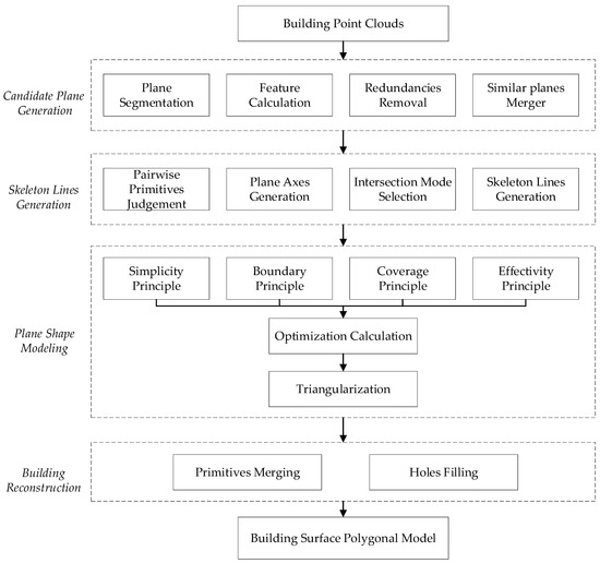
Figure 1.
The pipeline of the proposed method.
- (1)
- Candidate plane generation. The extraction of candidate plane primitives is the basis of all subsequent reconstruction processes. This work first employs a plane segmentation method to divide the point clouds into several plane pieces. Then, the features of these pieces are computed. Considering that some segmented pieces may be undesired elements, a process of elimination is applied to simplify the plane results. Additionally, some planes may be divided into multiple pieces due to the building complexity. Similar pieces are merged according to their features. Following these steps, a set of candidate plane primitives is obtained.
- (2)
- Skeleton lines generation. Models are made up of faces, faces are made up of lines, and lines are made up of points. Therefore, the key of framework reconstruction is to find the skeleton lines and their connecting points based on candidate planes primitives. In this part, an improved connection evaluation method is proposed. First, plane pairs are formed based on adjacent plane primitives. Then, plane axes are determined by considering the positional relationship between pairwise primitives. Subsequently, intersection modes are designated according to plane axes. Finally, skeleton lines are generated by combining plane intersection modes.
- (3)
- Plane shape modeling. Actually, not all skeleton lines are utilized in the creation of a plane model, owing to factors like the presence of some skeleton lines within the plane. Therefore, a framework-based optimization method is proposed, which converts the skeleton line selection problem into an optimal boundary loop selection problem. The optimization calculation incorporates four guiding principles: the simplicity principle, the boundary principle, the coverage principle, and the effectivity principle. After obtaining the optimal boundary loop, the plane is modeled through triangulation.
- (4)
- Building reconstruction. Based on the above plane primitive models, the final model can be obtained by merging primitive models and filling holes.
2.2. Candidate Plane Generation
The purpose of this section is to generate a reasonable set of candidate plane primitives CP (with a count of n) using the input building point clouds BP.
where is a candidate plane primitive.
Plane segmentation. This proposed method first divides building point clouds BP into many planar pieces PP (with a count of m) according to point normal vectors and point distances [21].
where is a set of points that are close enough and similar in direction.
Feature calculation. The number of points , ratio of length to width , normal vectors , and average color of each piece are calculated to prepare for subsequent redundancies removal and similar planes merger.
where is the feature values of .
Redundancies removal. Given the presence of numerous outliers in the building point clouds, the data may give rise to unnecessary pieces. Considering factors such as the overall number of point clouds, the uneven distribution of point clouds, and the shape of point pieces, the following pieces are deleted:
where represents pieces with point counts below a threshold , represents pieces located on the top of the building with point counts below a threshold , and represents pieces characterized by slender shapes with point counts below a threshold . The thresholds depend on the actual number of building point clouds.
Then, the remaining planar pieces are:
Similar planes merger. Using the features calculated through the feature calculation step, the similar planes can be judged [36]. This work presents two criteria for judging similar planes: 1. The normal vectors of the two point clouds are similar enough. 2. The ratio of length to width of one of the two point clouds is large enough, and the points in this point cloud are all close enough to the other point cloud. Among them, it is considered that condition 1 is more likely to explain the similarity than condition 2.
where represents two similar planes, while and , respectively, represent plane pairs that satisfy condition 1 and condition 2, is the threshold of the difference between two normal vectors, is the threshold of the difference between two ratios of length to width, is the maximum value of the nearest distances of points in to , and is the threshold of the distance.
Given that some small planes may be similar to multiple large planes, it is necessary to establish merging rules to judge the merging sort. Firstly, the distinction between primary and secondary relationships of point clouds becomes vital during the merging process. This work considers that the primary plane has the following characteristics relative to the secondary plane: 1. The ratio of length to width should not be too large. 2. The number of point clouds should be large. Then, the merging order can be determined as follows: 1. Plane pairs judged by condition 1 are preferentially merged. 2. Plane pairs with more similar colors are preferentially merged. After similar planes merge, a reasonable set of candidate plane primitives CP can be obtained.
As shown in Figure 2, for a building point clouds example, a sequence of steps is executed. After plane segmentation (arrow 1), multiple plane pieces are segmented. Following feature calculation, the redundant gray piece is removed through redundancies removal (arrow 2). Then, based on the calculated features, similar planes are merged (arrow 3). For example, the yellow and the red pieces can be merged according to condition 1, while the dark green and the light green pieces can be merged according to condition 2. Notably, even though the blue and the light green pieces also satisfy condition 2, the dark green piece is chosen due to its closer color similarity.
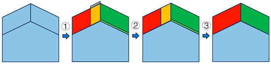
Figure 2.
Schematic diagram of candidate plane generation.
2.3. Skeleton Lines Generation
This section focuses on generating skeleton lines for each candidate plane primitive, which play a pivotal role in building modeling [37,38]. To effectively establish the topological connections between plane primitives, this work improves the connection evaluation method. The main improvement involves extracting the axes of two adjacent planes in any two orientations, subsequently determining the connection mode suitable for planar buildings according to the axes, and ultimately extracting and arranging essential skeleton lines.
Pairwise primitives judgement. Adjacency pairwise primitives are the basis of the connection evaluation method. This work uses the shortest Euclidean distances between the geometries to judge pairwise primitives [25]. To visually show the adjacency between planes, the adjacency graph shown in Figure 3 is usually used. In Figure 3, plane primitives of different colors first calculate their Euclidean distances from each other. When the distance approximates 0, it signifies adjacency between the two planes. Therefore, dotted lines link the center points of every two adjacent planes to complete the adjacency graph. The adjacent pairwise primitives AP in Figure 3 are .
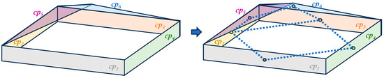
Figure 3.
Adjacency graph to show the pairwise primitives.
Plane axes generation. Based on the pairwise primitives, the connection relationship can be evaluated by the connection evaluation method. However, the connection evaluation methods are typically employed when the orientations of the wall axes remain constant [25]. In the case of buildings with complex planar orientation, different wall axes may be present when one plane faces different adjacent planes. Therefore, this work proposes a method to generate plane axes.
As shown in Figure 4a, for two planes and with center points and , their normal vectors and can be calculated. The normal vector of the plane that is perpendicular to both and is
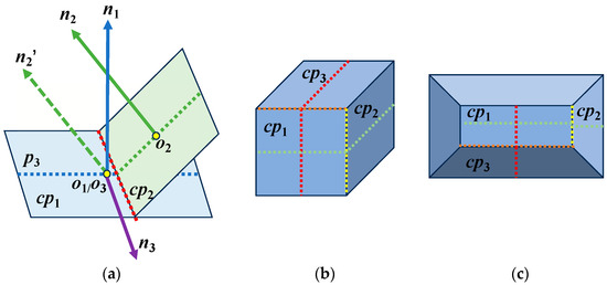
Figure 4.
Schematic diagram of plane axes generation: (a) plane axes calculation; (b) plane axes example A; (c) plane axes example B.
The point on the plane is
where Area(·) represents the size of the candidate plane primitive.
The equation of is
where are the direction ratios of the normal vector .
The current axis of can be obtained by solving the simultaneous equations of and , and likewise, the axis of can be obtained. The dotted blue line and the dotted green line in Figure 4a are the axes for and , respectively. The dotted red line in Figure 4a is the intersecting line between and .
Figure 4b,c are two examples showing that the axis of one plane can be different when facing different planes. Dotted green lines indicate the axes between and , while dotted red lines indicate the axes between and . Moreover, dotted yellow lines indicate the intersecting lines between and , while dotted orange lines indicate the intersecting lines between and .
Intersection mode selection. Considering the characteristics of planar buildings, this work adopts the direct intersection method [25] to achieve plane connections. For each pairwise plane primitive, to judge the effect of the intersecting line on every plane, the points in each plane are projected onto its axis to form a solid axis line, and the distance between the axis line and the intersecting line is calculated. As shown in the top row of Figure 5, due to the complexity of buildings and the point cloud noise and loss, there are many possibilities for point clouds and their projected lines on the two planes.
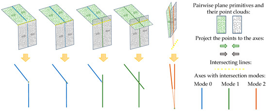
Figure 5.
Examples of intersection mode selection.
Using the distance relationship between the plane axis and the intersecting line, the intersection mode of each plane can be determined. Three types of intersection mode are chosen, as shown in different colors of the solid axis lines in Figure 5. The bottom row of Figure 5 is a simplified version of the top row, three colors mean different intersection modes for the current planes, and the yellow circles mean the intersection positions.
Firstly, when one end of the solid line is very close to the intersection point, it is considered that the other plane may be a truncation of the current plane. For the blue lines in Figure 5, this work uses mode 0 to indicate that the current plane is truncated. Secondly, when one end of the solid line exceeds a certain range of the intersection point, it is considered that the other plane may only reach the middle of the current plane. For the green lines in Figure 5, this work uses mode 1 to indicate that the current plane is not truncated. Thirdly, when one end of the solid line exceeds the intersection point a lot, it is considered that the two planes may be close to parallel. For the orange lines in Figure 5, this work uses mode 2 to indicate plane parallelism, which is no longer used for skeleton line generation.
Skeleton lines generation. In this work, the intersecting lines of reasonable length belonging to the current plane are defined as skeleton lines, which are subsequently processed as the boundaries of the current plane. Therefore, two different lengths of intersecting line segments and can be obtained by projecting the point clouds of two planes corresponding to the intersecting line onto the intersecting line. As illustrated in Figure 6, for the current pairwise and , the preceding procedures yield two axes (the black dotted line and the red dotted line), one intersecting line (the purple dotted line), two intersecting line segments (the yellow line segment and the green line segment), and the respective intersection mode for each plane (mode 0 and mode 0).
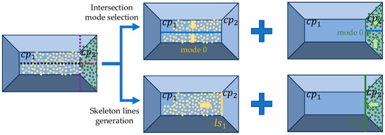
Figure 6.
Contrast diagram of intersection modes and skeleton lines.
Therefore, for each plane primitive , intersecting with distinct planes results in the acquisition of a set of intersecting line segment pairs :
where
Since each contains two segments of different lengths, two sets of potential skeleton lines can be obtained:
in which
where Long(·) and Short(·) represent the longer and the shorter segments of the two segments, respectively.
An example of and is shown in Figure 7, where the blue segments denote an intersection mode of 0, and the green segments denote an intersection mode of 1.
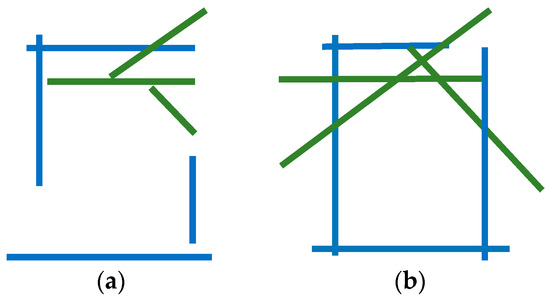
Figure 7.
Example of potential skeleton line sets: (a) an example of ; (b) an example of .
Similar to the intersection mode selection process of determining whether there are intersection points of axes, by calculating the shortest distance between every two segments in the same skeleton line sets, this work evaluates whether a potential intersection point exists between them. Then, the boundary constraint of segments is carried out by using the intersection point positions and the intersection modes. Figure 8a,b show and after the intersection point generation and boundary constraint, in which the yellow points represent the intersection points and the green points represent endpoints without constraint. To generate a unified set of potential skeleton lines, this work uses as the basis and uses to further modify the uncertain endpoints. Finally, the remaining uncertain endpoints are connected to the nearest noncollinear intersection points to complete the closed skeleton lines generation. Figure 8c shows the combination of constrained and , and Figure 8d shows the final skeleton lines. Notably, in Figure 8d, each intersection point is related to at least two line segments.
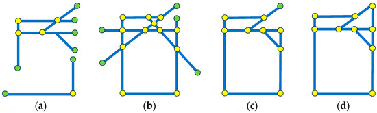
Figure 8.
Example of potential skeleton line sets after processing: (a) after constraint; (b) after constraint; (c) initial combination and (d) final skeleton lines.
2.4. Plane Shape Modeling
This section proposes a plane shape optimization method based on topological connection principles, which converts the plane modeling task into an optimal boundary closed-loop selection problem. Given K skeleton line segments SL = {} generated in the previous step, this work selects a subset of these line segments to form the triangulation model of the current plane.
Topological connection principles. We define four principles to compose our objective function:
Simplicity principle. The number of intersection points in the selected loop should be as small as possible. Therefore, the ratio of the total number of intersection points in the closed loop to the total number of intersection points in the skeleton lines is calculated as the first numerical term .
Boundary principle. The closed loop should be made up of boundary lines with a truncation effect to the greatest extent. Considering that the intersection mode can reflect whether the plane is truncated, the ratio of the total number of mode values in the closed loop to the total number of mode values in the skeleton lines is calculated as the second numerical term .
Coverage principle. As many point clouds as possible in the current plane should be contained in the closed loop. Consequently, the ratio of the total number of point clouds contained in the closed loop to the total number of point clouds belong to the current plane is calculated. To optimize the indicators uniformly, this work uses one minus the ratio value as the third numerical term .
Effectivity principle. The regions without point clouds in the closed loop should be as small as possible. Accordingly, the ratio of the region containing point clouds in the closed loop to the region of the total closed loop is calculated. This work uses one minus the ratio value as the fourth numerical term .
Optimization calculation. Based on the skeleton line sets, different simple undirected closed loops SUCL can be obtained [39], where each intersection point on the closed loop is a 2-link point (the point connects to two line segments).
where represents a closed loop and M is the number of closed loops.
Using the above four principles, this work calculates the framework optimization value of each loop and chooses the loop with the smallest value as the result RV.
where , , , and represent weights of different numerical terms and +++, min(·) represents choosing the smallest value.
The adjustment of a weight represents a change in the importance attached to the corresponding principle. A high weight indicates that the current principle plays an important role in the loop selection. A high indicates a simple loop rather than unnecessary turns, but it may also cause a small plane. A high indicates that the skeleton lines are close to the point cloud boundary but may lead to a complex loop. A high indicates a sufficient point cloud coverage, but the plane may be larger than the true plane due to outliers and other reasons. A high indicates that the plane basically fits the point cloud, but the plane may be smaller than the true plane due to the absence of the point cloud. Therefore, by adjusting the weights, the loops can be modified according to specific needs. In addition, for the balance of principles, the values of the four weights are not exactly equal. This is due to the small numbers of skeleton lines and intersections in the plane, resulting in relatively discrete changes in and . On the contrary, changes in and caused by changes in the point numbers and region area are relatively continuous. Therefore, to avoid the relatively large impact of changes in and , and should be smaller than and .
Triangularization. After the optimal simple undirected closed loop is obtained, the model of the current plane primitive can be obtained by triangulating the closed loop [40].
As shown in Figure 9, a collection of potential simple undirected closed loops is initially calculated from a set of skeleton lines. Utilizing the four principles as guidelines, an optimal closed loop is derived, striving to encompass the majority of point clouds. Finally, the triangular mesh model of the plane is generated through triangulation.
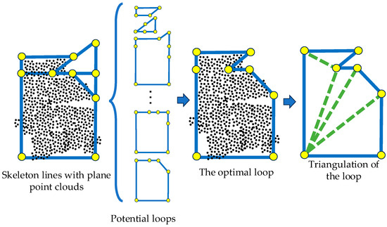
Figure 9.
Schematic diagram of plane shape modeling.
2.5. Building Reconstruction
Based on the above steps, models for each plane are obtained. By aligning these plane models with their original spatial positions, the collective model of all planes can be seamlessly interconnected. However, some holes might emerge due to factors such as the selection of closed loops. This work fills the holes based on the existing skeleton lines and intersection points. With the completion of all stages, the 3D reconstruction of the building is successfully achieved.
3. Experiments
To evaluate the proposed approach, a building is taken as an example to give the whole process result of modeling. Then, this work qualitatively and quantitatively compares the reconstruction quality of different buildings with those of some SOTA methods. Experiments demonstrated the advantages of our hybrid method of connection evaluation and framework optimization for building surface reconstruction. In this section, experimental comparisons are made with SOTA traditional methods and deep learning methods, respectively, and two kinds of metrics are used to verify simplicity and accuracy. Moreover, to demonstrate the superiority of the proposed method in the 3D reconstruction of buildings, this work further illustrates the application based on the model result. Taking a building as an example, a textural model and LOD3 model based on the surface model are constructed. The results are shown below.
3.1. Data and Metrics Selection
3.1.1. Experimental Data
The method in this paper can reconstruct piecewise planar buildings. To qualitatively and quantitatively analyze the proposed method, several real-world buildings with different shapes and complexity are chosen as shown in Figure 10 (buildings 1–6). The photogrammetric point clouds are generated from oblique photography images of typical modern buildings captured in the suburban areas of China. Among buildings 1–6, buildings 1–4 are captured in Beijing and buildings 5–6 are captured in Zhuhai. Image orientation and point cloud generation are obtained by existing solutions including structure form motion (SFM) and multi-view stereo (MVS). The descriptions of the photogrammetric surveys employed for the experiments and their characteristics are shown in Table 1. The major components of buildings in the point clouds are visible, yet there remains some noise and absence of the point clouds due to the factors such as shooting heights and occlusions. As for the comparison experiment with the deep learning algorithm proposed in Building3D [35], in order to avoid the difference caused by different data characteristics, three buildings in the dataset of the original paper are used for comparison, as shown in Figure 10 (buildings 7–9). Notably, the point clouds in Building3D are laser point clouds instead of photogrammetric point clouds, which are not our focus. In addition, to well display the characteristics of the buildings, scalebars and coordinate axes are shown below the building point clouds in Figure 10, and the unit of the scalebars is meter (m).
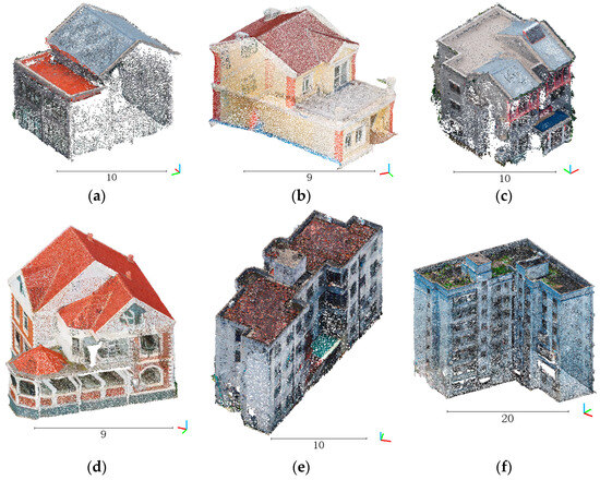
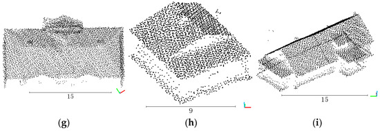
Figure 10.
Building point clouds. (a) Photogrammetric point cloud building 1; (b) photogrammetric point cloud building 2; (c) photogrammetric point cloud building 3; (d) photogrammetric point cloud building 4; (e) photogrammetric point cloud building 5; (f) photogrammetric point cloud building 6; (g) Building3D point cloud building 7; (h) Building3D point cloud building 8; (i) Building3D point cloud building 9.

Table 1.
Photogrammetric characteristics.
Moreover, according to the method proposed in Section 2, thresholds , , , , , and and weights , , , and need to be set before the experiments take place. After an experimental comparison of the visual and data effects of different values of these factors, the thresholds and weights are set as shown in Table 2. It is worth noting that the values can be modified according to the actual conditions of the building.
Table 2.
Thresholds and weights settings.
3.1.2. Metrics Selection
To quantitatively analyze the modeling effect, this work adopts metrics of two aspects to assess reconstruction performance, which are simplicity and accuracy.
The first aspect pertains to the simplicity of the models. Since the objective is to create lightweight polygonal models, the number of vertices (Ver. No.) and the number of faces (Fac. No.) in the model become critical evaluation factors. Taking building 1 we mentioned in Section 3.1.1 as an example, Figure 11a represents the built 3D model, Figure 11b represents the vertices on the model (each point is a sphere), Figure 11c represents the wireframe of the model, and Figure 11d represents the faces based on the wireframe (each face is a triangular face). The small numbers of vertices and faces signify the simple reconstruction model. This work uses the software CloudCompare to count the number of vertices and faces. After importing the model into CloudCompare, the number of vertices can be obtained through “Cloud” and the number of faces can be obtained through “Mesh” in column “Properties”. The units of vertices and faces are both individual.
Figure 11.
Examples of vertices and faces of a model. (a) 3D model; (b) vertices on the model; (c) wireframe of the model; (d) faces based on the wireframe.
The second aspect concerns the accuracy of the models. This work mainly uses the orthogonal distance from the original building points to their nearest faces of the building 3D model (P2M) and the shortest distance from the building model vertices to the original building points (O2P) to assess the model accuracy [15,16]. Taking building 1 we mentioned in Section 3.1 as an example, Figure 12a represents the combination of the input point clouds and the built 3D model, Figure 12b represents the P2M distance of each point in the point clouds, Figure 12c represents the combination of the input point clouds and the building model vertices, and Figure 12d represents the O2P distance of each building model vertex. For an intuitive comparison, this work calculates the mean P2M distance (Mean P2M) and the mean O2M distance (Mean O2P). Moreover, for a mean P2M distance, the lower the value, the higher the fit degree between the input point clouds and the output model mesh. For a mean O2M distance, the lower the value, the fewer artificial points exist and the more accurate the retention of key features. Therefore, both low values indicate accurate results. The mean P2M distance and the mean O2P distance can also be calculated using the software CloudCompare. After importing the model and the original point cloud into CloudCompare, we can use “Tools”-“Distances”-“Mesh”-“Cloud/Mesh Dist.” and “Cloud/Cloud Dist.” to calculate the mean P2M distance and the mean O2P distance. The unit for both P2M and O2P is meter (m). meter (m) is also the unit of the scalebars in Figure 12.
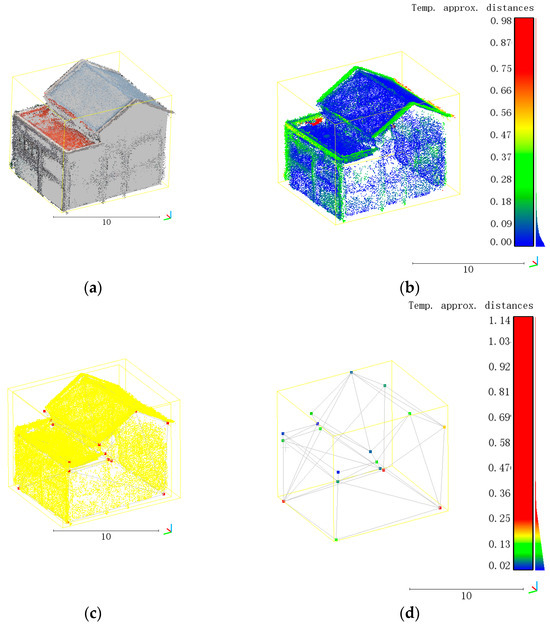
Figure 12.
Examples of P2M and O2P of a model. (a) Point clouds and 3D model; (b) P2M distance of each point; (c) point clouds and model vertices; (d) O2P distance of each model vertex.
3.2. Modeling Result Example
To explain the experimental results of each step in the modeling process, the modeling process diagram is given with building 1 as an example.
As shown in Figure 13, in the candidate plane generation step, the building point cloud (a) is segmented first. However, some point cloud parts in the segmentation result are not suitable for modeling alone, such as the red dotted box parts in (b). After redundancies are removed and similar planes are merged, a relatively satisfactory result (c) can be obtained.
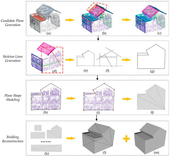
Figure 13.
The modeling process diagram of building 1.
Based on the candidate planes, in the skeleton lines generation step, a pairwise intersection is used to find the potential skeleton lines of the building. Taking the plane in the red dotted box in (d) and its two adjacent planes as an example, two intersection lines (the black lines in (d)) can be calculated. Moreover, according to the condition of the axes of the plane (the green lines and the red lines in (d)) when intersecting, the mode of each intersection is judged, which will be used in subsequent loop selection. After calculating all the intersection relations of the current plane, and ((e) and (f)) can be obtained to generate the final skeleton lines (g). Notably, the final skeleton lines are not simple enough, which should be further selected for modeling.
In the plane shape modeling step, by combining the situations of the point cloud and the skeleton lines (h), this work calculates the optimal loop (i) for modeling. The optimal loop not only can fit the point cloud basically but also is easy to triangulate. This is useful for obtaining a correct and simple mesh model.
Finally, this work combines models of different planes to achieve building reconstruction.
3.3. Comparison with Traditional Methods
To demonstrate the advances of our method, this work conducts experiments with two SOTA traditional building surface reconstruction methods, namely the 2.5D dual contouring method (2.5DC) [41] and the PolyFit method [42].
3.3.1. Modeling Results and Qualitative Analysis
Table 3 shows the reconstruction results of the three methods of buildings 1–6.
Table 3.
Reconstruction results comparison with traditional methods.
From the above visual effects of different reconstruction results, it can be seen that these methods can all obtain the polygonal surface models of buildings. Among them, the 2.5DC method mainly reconstructs point clouds by identifying building roofs and then extruding them to create the models. Although the major components can be retained, the framework information is ignored. In addition, the 2.5DC method performs poorly on flat surfaces, which hampers subsequent steps such as texture mapping. Regarding the PolyFit method, it can produce flat polygonal surface models and offer building framework information. However, due to the requirements of manifold and watertight models, along with some limitations in model optimization settings, some model details can be overly simplified. The method in this work is grounded in planes, and the framework is modeled by exploring the connection between these planes. Polygonal models of planes are then constructed using optimization equations. Consequently, this method preserves plane feature information to a great extent while also ensuring the correctness of the model framework.
3.3.2. Quantitative Analysis
The simplicity results for the six buildings in Section 3.3.1 are shown in Table 4. The results are the numbers of vertices and faces.
Table 4.
Simplicity results comparison with traditional methods.
Table 4 shows that the proposed method can achieve the lowest numbers of vertices and faces of the three methods. Through the method analysis, it can be seen that the main reason for the large numbers of vertices and faces of 2.5DC is that their planes are not flat enough, while the main reason for the large numbers of vertices and faces of PolyFit is that their faces in a plane are too fragmented. For the method proposed in this paper, because the optimal closed loop is found for each plane and the triangular mesh is constructed based on the intersection points of the closed loop, it can not only ensure the flatness of the plane but also ensure there is as little segmentation as possible on the surface.
Table 5 shows the accuracy results of the three methods, where the unit of distances is meter (m).
Table 5.
Accuracy results comparison with traditional methods.
As can be seen from the simplicity validation, the proposed method has small numbers of faces and vertices, which results in the faces covering large areas and the vertices being distributed at the edges of models. In fact, the photogrammetric point clouds are not perfectly flat but undulating, which can result in less-than-ideal face fits. Moreover, when the vertices are distributed at the edges of models rather than in the middle of the planes, the mean O2P value might be higher because there are no central vertices to provide averaging. However, despite these considerations, the experimental results show that on the whole, the mean P2M and O2P data generated by the proposed method are still more accurate compared to other methods. Furthermore, there is no significant deviation in the data, which further underscores the stability and reliability of the proposed method.
3.4. Comparison with Deep Learning Methods
Considering the constant development of deep learning algorithms, this work also conducts experiments with two SOTA deep learning 3D reconstruction methods, namely the IGR method [33] and the Building3D method [35]. Notably, the IGR method is not designed only for buildings; therefore, this work reconstructs buildings 1–6 for comparison. As for the Building3D method, because different types of buildings have different data characteristics, and the Building3D method is mainly aimed at laser point clouds, buildings 7–9 provided in the Building3D dataset are selected for comparison. Moreover, because IGR has too many grids, and Building3D have an uneven surface, only 3D models are displayed for a more intuitive display. The comparison results with the two deep learning methods are shown separately as follows.
3.4.1. Comparison Results with IGR
Table 6 shows the reconstruction comparison results of the IGR method and the proposed method for buildings 1–6.
Table 6.
Reconstruction results comparison between IGR and our method.
Table 7 shows the simplicity comparison results of the IGR method and the proposed method for buildings 1–6. The results are the numbers of vertices and faces.
Table 7.
Simplicity results comparison between IGR and our method.
Table 8 shows the accuracy comparison results of the IGR method and the proposed method for buildings 1–6. The unit of accuracy results is meter (m).
Table 8.
Accuracy results comparison between IGR and our method.
From the above results, it can be seen that the reconstruction results of the IGR method are more consistent with the point clouds, and the mean P2M and mean O2P values of IGR are lower than the method proposed in this work. However, the IGR method builds complex mesh models, which not only results in a very high number of vertices and faces but also can lead to unwanted tortuous meshes and even some distortion due to noise points. Moreover, the goal of this work is to build LOD2 mesh models, which can be further used to build textural models and LOD3 models. Therefore, the simple mesh model is suitable for building subsequent models, and this work gives an application example in Section 3.5.
3.4.2. Comparison Results with Building3D
Table 9 shows the reconstruction comparison results of the Building3D method and the proposed method for buildings 7–9.
Table 9.
Reconstruction results comparison between Building3D and our method.
Table 10 shows the simplicity comparison results of the Building3D method and the proposed method for buildings 7–9. The results are the numbers of vertices and faces.
Table 10.
Simplicity results comparison between Building3D and our method.
Table 11 shows the accuracy comparison results of the Building3D method and the proposed method for buildings 7–9. The unit of accuracy results is meter (m).
Table 11.
Accuracy results comparison between Building3D and our method.
Building3D adopts self-supervised pre-training methods for 3D building reconstruction and can build simple LOD2 mesh models. However, because Building3D does not take into account the actual framework of the buildings, some models have uneven surfaces. Uneven surfaces not only pose potential problems for subsequent steps such as texture mapping but also increase the number of faces. Since the proposed method is based on the plane point cloud for surface reconstruction, each plane retains the topological structure characteristics well. The reconstructed results of the proposed method not only look closer to the actual situation but also show smaller mean P2M and O2P values.
3.5. Application
Since the proposed method uses aerial images to generate point clouds through an SFM algorithm, the correspondence between point clouds and images can be obtained, enabling texture mapping. In addition, the skeletons are extracted after plane fitting based on point cloud segmentation, which can not only determine the topological relationship between planes but also facilitate the clipping of flat texture images. The flat texture images ensure that the building is not distorted, and the components can be extracted for LOD3 reconstruction. In order to illustrate the application of our method in CityGML, this work takes building 1 as an example to build a textural model and LOD3 model. The results are shown in Figure 14.
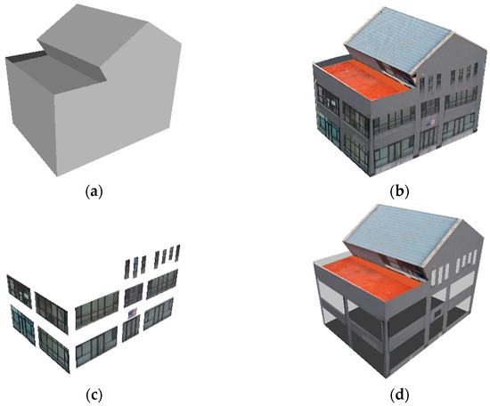
Figure 14.
Model of CityGML. (a) LOD2 3D model; (b) LOD2 textural model; (c) LOD3 component models; (d) LOD3 model without components.
From the above results, it can be seen that the model built by the proposed method can generate satisfying LOD2 textural and LOD3 models, which is closely related to the plane fitting and topological relationship detecting carried out by the photogrammetric point cloud in this work.
4. Discussion
This work proposes a workflow for obtaining a building surface reconstruction characterized by low numbers of vertices and faces as well as a relatively good performance regarding model accuracy. The proposed method is based on the definition of candidate planes from the building point cloud, and it especially describes methods of extracting intersection lines of arbitrarily oriented planes and optimizing the framework using intersection modes and the data.
The hybrid method that combines connection evaluation and framework optimization for building surface reconstruction has proven effective in creating 3D models from photogrammetric point clouds, which can be further used to build LOD3 models. Moreover, the modeling effect of this method on laser scanning point clouds is also verified.
However, since its preprocessing steps involve point cloud segmentation and plane fitting, the proposed method relies on the connection relationship between planes. Consequently, for this method to work optimally, it necessitates that the input data can extract planes as complete content as possible to avoid situations where the planes cannot be connected.
5. Conclusions
This work proposes a hybrid method of connection evaluation and framework optimization for building surface reconstruction from photogrammetric point clouds. Given the point clouds of a single planar building, a candidate plane generation method is firstly proposed to remove redundancies and merge similar elements to solve the poor effect of plane primitive extraction. Secondly, through the improvement of the connection evaluation method, this work solves the problem of connecting two plane primitives in any direction, and the skeleton lines of each plane are extracted. Thirdly, the plane modeling task is converted into an optimal boundary loop selection problem to realize plane shape modeling. Finally, by plane primitive merging and holes filling, a complete 3D building model is generated.
Experiment comparisons of our method with SOTA methods prove the qualitative and quantitative advantages of the proposed method in 3D building reconstruction. Reconstruction results and qualitative analysis demonstrate that the proposed method can reproduce the details while maintaining the major structure of the building. Meanwhile, quantitative analysis reveals that the proposed method can build simple models while ensuring the accuracy of modeling. Moreover, constructing a textural model and LOD3 model on the basis of a 3D model also shows the superiority of this work.
Although this work proposes a candidate plane generation method, the modeling results still rely on the initial plane segmentation. This reliance on the segmentation process is a common problem encountered in primitive-based methods. If there is a significant lack of data, addressing how to complete the modeling becomes a critical challenge that needs to be tackled in future research. This could involve developing robust methods for handling incomplete or sparse data and exploring techniques for data augmentation to improve the modeling process. In addition, for some buildings with curved parts, how to apply some of the steps in this work, such as skeleton line extraction, to other modeling algorithms, such as deep learning algorithms, will also be the focus of future research. Through the fusion of different algorithms, it may be possible to obtain a simple polygonal surface model on the basis of preserving the original topological relationship between curved and flat surfaces. Finally, to obtain the high LOD model, adding semantic, material, structure and other information on the polygon surface model is also future research content. On this basis, it is hoped that more building simulations can be further carried out.
Author Contributions
Conceptualization, Y.L., G.G. and N.L.; methodology, Y.L., C.L.(Chen Liu), G.G. and N.L.; software, Y.L., Y.Z. and Y.Q.; validation, Y.L. and C.L.(Chuanchuan Lu); writing—original draft preparation, Y.L.; writing—review and editing, G.G. and N.L. All authors have read and agreed to the published version of the manuscript.
Funding
This research funding is not publicly available due to privacy.
Data Availability Statement
The data presented in this study are available on request from the corresponding author. The data are not publicly available due to privacy.
Conflicts of Interest
The authors declare no conflicts of interest.
References
- Zhang, P.; He, H.; Wang, Y.; Liu, Y.; Lin, H.; Guo, L.; Yang, W. 3D urban buildings extraction based on airborne lidar and photogrammetric point cloud fusion according to U-Net deep learning model segmentation. IEEE Access 2022, 10, 20889–20897. [Google Scholar] [CrossRef]
- Pantoja-Rosero, B.G.; Achanta, R.; Kozinski, M.; Fua, P.; Perez-Cruz, F.; Beyer, K. Generating LOD3 building models from structure-from-motion and semantic segmentation. Autom. Constr. 2022, 141, 104430. [Google Scholar] [CrossRef]
- Kushwaha, S.; Mokros, M.; Jain, K. Enrichment of Uav Photogrammetric Point Cloud To Enhance Dsm in a Dense Urban Region. Int. Arch. Photogramm. Remote Sens. Spat. Inf. Sci. 2022, 48, 83–88. [Google Scholar] [CrossRef]
- Özdemir, E.; Remondino, F. Segmentation of 3D photogrammetric point cloud for 3D building modeling. Int. Arch. Photogramm. Remote Sens. Spat. Inf. Sci. 2018, 42, 135–142. [Google Scholar] [CrossRef]
- Tan, Y.; Liang, Y.; Zhu, J. CityGML in the Integration of BIM and the GIS: Challenges and Opportunities. Buildings 2023, 13, 1758. [Google Scholar] [CrossRef]
- Saran, S.; Wate, P.; Srivastav, S.; Krishna Murthy, Y. CityGML at semantic level for urban energy conservation strategies. Ann. GIS 2015, 21, 27–41. [Google Scholar] [CrossRef]
- Boeters, R.; Arroyo Ohori, K.; Biljecki, F.; Zlatanova, S. Automatically enhancing CityGML LOD2 models with a corresponding indoor geometry. Int. J. Geogr. Inf. Sci. 2015, 29, 2248–2268. [Google Scholar] [CrossRef]
- Ying, L.; Guanghong, G.; Lin, S. A fast, accurate and dense feature matching algorithm for aerial images. J. Syst. Eng. Electron. 2020, 31, 1128–1139. [Google Scholar] [CrossRef]
- Jiang, Y.; Dai, Q.; Min, W.; Li, W. Non-watertight polygonal surface reconstruction from building point cloud via connection and data fit. IEEE Geosci. Remote Sens. Lett. 2021, 19, 1–5. [Google Scholar] [CrossRef]
- Buyukdemircioglu, M.; Kocaman, S.; Kada, M. Deep learning for 3D building reconstruction: A review. Int. Arch. Photogramm. Remote Sens. Spat. Inf. Sci. 2022, 43, 359–366. [Google Scholar] [CrossRef]
- Chen, Z.; Xiang, X.; Zhou, H.; Hu, T. Data-driven Reconstruction for Massive Buildings within Urban Scenarios: A Case Study. In Proceedings of the 2020 IEEE 9th Data Driven Control and Learning Systems Conference (DDCLS), Liuzhou, China, 20–22 November 2020; pp. 982–988. [Google Scholar]
- Murtiyoso, A.; Veriandi, M.; Suwardhi, D.; Soeksmantono, B.; Harto, A.B. Automatic Workflow for Roof Extraction and Generation of 3D CityGML Models from Low-Cost UAV Image-Derived Point Clouds. ISPRS Int. J. Geo-Inf. 2020, 9, 743. [Google Scholar] [CrossRef]
- Huang, W.; Jiang, S.; Jiang, W. A model-driven method for pylon reconstruction from oblique UAV images. Sensors 2020, 20, 824. [Google Scholar] [CrossRef]
- Costantino, D.; Vozza, G.; Alfio, V.S.; Pepe, M. Strategies for 3D Modelling of Buildings from Airborne Laser Scanner and Photogrammetric Data Based on Free-Form and Model-Driven Methods: The Case Study of the Old Town Centre of Bordeaux (France). Appl. Sci. 2021, 11, 10993. [Google Scholar] [CrossRef]
- Liu, X.; Zhang, Y.; Ling, X.; Wan, Y.; Liu, L.; Li, Q. TopoLAP: Topology recovery for building reconstruction by deducing the relationships between linear and planar primitives. Remote Sens. 2019, 11, 1372. [Google Scholar] [CrossRef]
- Xie, L.; Hu, H.; Zhu, Q.; Li, X.; Tang, S.; Li, Y.; Guo, R.; Zhang, Y.; Wang, W. Combined rule-based and hypothesis-based method for building model reconstruction from photogrammetric point clouds. Remote Sens. 2021, 13, 1107. [Google Scholar] [CrossRef]
- Monszpart, A.; Mellado, N.; Brostow, G.J.; Mitra, N.J. RAPter: Rebuilding man-made scenes with regular arrangements of planes. ACM Trans. Graph. 2015, 34, 103:101–103:112. [Google Scholar] [CrossRef]
- Schnabel, R.; Wahl, R.; Klein, R. Efficient RANSAC for point-cloud shape detection. In Computer Graphics Forum; Wiley: Hoboken, NJ, USA, 2007; pp. 214–226. [Google Scholar]
- Ma, X.; Luo, W.; Chen, M.; Li, J.; Yan, X.; Zhang, X.; Wei, W. A fast point cloud segmentation algorithm based on region growth. In Proceedings of the 2019 18th International Conference on Optical Communications and Networks (ICOCN), Huangshan, China, 5–8 August 2019; pp. 1–2. [Google Scholar]
- Lu, X.; Yao, J.; Tu, J.; Li, K.; Li, L.; Liu, Y. Pairwise linkage for point cloud segmentation. ISPRS Ann. Photogramm. Remote Sens. Spat. Inf. Sci. 2016, 3, 201–208. [Google Scholar] [CrossRef]
- Nguyen, A.; Le, B. 3D point cloud segmentation: A survey. In Proceedings of the 2013 6th IEEE Conference on Robotics, Automation and Mechatronics (RAM), Manila, Philippines, 12–15 November 2013; pp. 225–230. [Google Scholar]
- Wang, B.; Wu, G.; Zhao, Q.; Li, Y.; Gao, Y.; She, J. A topology-preserving simplification method for 3d building models. ISPRS Int. J. Geo-Inf. 2021, 10, 422. [Google Scholar] [CrossRef]
- Abou Diakité, A.; Damiand, G.; Van Maercke, D. Topological reconstruction of complex 3d buildings and automatic extraction of levels of detail. In Proceedings of the Eurographics Workshop on Urban Data Modelling and Visualisation, Strasbourg, France, 6 April 2014; pp. 25–30. [Google Scholar]
- He, B.; Li, L.; Guo, R.; Shi, Y. 3D topological reconstruction of heterogeneous buildings considering exterior topology. Geomat. Inf. Sci. Wuhan Univ. 2011, 36, 579–583. [Google Scholar]
- Bassier, M.; Vergauwen, M. Topology reconstruction of BIM wall objects from point cloud data. Remote Sens. 2020, 12, 1800. [Google Scholar] [CrossRef]
- Previtali, M.; Scaioni, M.; Barazzetti, L.; Brumana, R. A flexible methodology for outdoor/indoor building reconstruction from occluded point clouds. ISPRS Ann. Photogramm. Remote Sens. Spat. Inf. Sci. 2014, 2, 119–126. [Google Scholar] [CrossRef]
- Mathias, M.; Martinovic, A.; Weissenberg, J.; Van Gool, L. Procedural 3D building reconstruction using shape grammars and detectors. In Proceedings of the 2011 International Conference on 3D Imaging, Modeling, Processing, Visualization and Transmission, Hangzhou, China, 16–19 May 2011; pp. 304–311. [Google Scholar]
- Li, Z.; Shan, J. RANSAC-based multi primitive building reconstruction from 3D point clouds. ISPRS J. Photogramm. Remote Sens. 2022, 185, 247–260. [Google Scholar] [CrossRef]
- Song, J.; Xia, S.; Wang, J.; Chen, D. Curved buildings reconstruction from airborne LiDAR data by matching and deforming geometric primitives. IEEE Trans. Geosci. Remote Sens. 2020, 59, 1660–1674. [Google Scholar] [CrossRef]
- Müller, P.; Wonka, P.; Haegler, S.; Ulmer, A.; Van Gool, L. Procedural modeling of buildings. In Proceedings of the SIGGRAPH06: Special Interest Group on Computer Graphics and Interactive Techniques Conference, Boston, MA, USA, 30 July–3 August 2006; pp. 614–623. [Google Scholar]
- Murali, S.; Speciale, P.; Oswald, M.R.; Pollefeys, M. Indoor Scan2BIM: Building information models of house interiors. In Proceedings of the 2017 IEEE/RSJ International Conference on Intelligent Robots and Systems (IROS), Vancouver, BC, Canada, 24–28 September 2017; pp. 6126–6133. [Google Scholar]
- Jung, J.; Stachniss, C.; Ju, S.; Heo, J. Automated 3D volumetric reconstruction of multiple-room building interiors for as-built BIM. Adv. Eng. Inform. 2018, 38, 811–825. [Google Scholar] [CrossRef]
- Gropp, A.; Yariv, L.; Haim, N.; Atzmon, M.; Lipman, Y. Implicit geometric regularization for learning shapes. arXiv 2020, arXiv:2002.10099. [Google Scholar]
- Bacharidis, K.; Sarri, F.; Ragia, L. 3D building façade reconstruction using deep learning. ISPRS Int. J. Geo-Inf. 2020, 9, 322. [Google Scholar] [CrossRef]
- Wang, R.; Huang, S.; Yang, H. Building3D: A Urban-Scale Dataset and Benchmarks for Learning Roof Structures from Point Clouds. In Proceedings of the IEEE/CVF International Conference on Computer Vision, Paris, France, 1–6 October 2023; pp. 20076–20086. [Google Scholar]
- Yang, B.; Dong, Z. A shape-based segmentation method for mobile laser scanning point clouds. ISPRS J. Photogramm. Remote Sens. 2013, 81, 19–30. [Google Scholar] [CrossRef]
- Sugihara, K. Straight Skeleton Computation Optimized for Roof Model Generation. In WSCG; Václav Skala-UNION Agency: Pilsen, Czech Republic, 2019; pp. 101–109. [Google Scholar]
- Sugihara, K.; Kikata, J. Automatic generation of 3D building models from complicated building polygons. J. Comput. Civ. Eng. 2013, 27, 476–488. [Google Scholar] [CrossRef][Green Version]
- Johnson, D.B. Finding all the elementary circuits of a directed graph. SIAM J. Comput. 1975, 4, 77–84. [Google Scholar] [CrossRef]
- Bern, M.; Shewchuk, J.R.; Amenta, N. Triangulations and mesh generation. In Handbook of Discrete and Computational Geometry; Chapman and Hall/CRC: Boca Raton, FL, USA, 2017; pp. 763–785. [Google Scholar]
- Zhou, Q.-Y.; Neumann, U. 2.5 d dual contouring: A robust approach to creating building models from aerial lidar point clouds. In Proceedings of the Computer Vision–ECCV 2010: 11th European Conference on Computer Vision, Heraklion, Crete, Greece, 5–11 September 2010; pp. 115–128. [Google Scholar]
- Nan, L.; Wonka, P. Polyfit: Polygonal surface reconstruction from point clouds. In Proceedings of the IEEE International Conference on Computer Vision, Venice, Italy, 22–29 October 2017; pp. 2353–2361. [Google Scholar]


Disclaimer/Publisher’s Note: The statements, opinions and data contained in all publications are solely those of the individual author(s) and contributor(s) and not of MDPI and/or the editor(s). MDPI and/or the editor(s) disclaim responsibility for any injury to people or property resulting from any ideas, methods, instructions or products referred to in the content. |
© 2024 by the authors. Licensee MDPI, Basel, Switzerland. This article is an open access article distributed under the terms and conditions of the Creative Commons Attribution (CC BY) license (https://creativecommons.org/licenses/by/4.0/).