Abstract
The full waveform inversion at this stage still has many problems in the recovery of deep background velocities. Velocity modeling based on end-to-end deep learning usually lacks a generalization capability. The proposed method is a multi-scale convolutional neural network velocity inversion (Ms-CNNVI) that incorporates a multi-scale strategy into the CNN-based velocity inversion algorithm for the first time. This approach improves the accuracy of the inversion by integrating a multi-scale strategy from low-frequency to high-frequency inversion and by incorporating a smoothing strategy in the multi-scale (MS) convolutional neural network (CNN) inversion process. Furthermore, using angle-domain reverse time migration (RTM) for dataset construction in Ms-CNNVI significantly improves the inversion efficiency. Numerical tests showcase the efficacy of the suggested approach.
1. Introduction
Seismic exploration depends heavily on modeling velocity, as it directly impacts downstream data processing accuracy. As such, this area of research has received considerable attention and continues to be a critical aspect of seismic exploration. Velocity modeling in seismic exploration encompasses several methods including migration velocity analysis [1], tomography [2], and full-waveform inversion (FWI) [3,4,5]. The aim of these techniques is to produce high-resolution velocity models [6] that can provide valuable insight into subsurface geological structures and enable accurate seismic imaging and interpretation.
As the most advanced seismic inversion technique, FWI (or full-waveform inversion) aims to generate high-resolution models of subsurface media by iteratively fitting the observed waveform, which enables us to extract more information from seismic data and create highly detailed velocity models. Due to the influence of the shallow tomographic component (mainly direct and diving waves), FWI mainly updates the velocity information in the shallow layers, but hardly addresses the deep layers. Reflection-waveform inversion (RWI) [7,8,9,10,11,12,13,14], developed on this basis, updates the deep layer background velocity. However, it is still difficult to update the complex structural features of the deeper layers. The difficulty of updating deep velocity features is a bottleneck in waveform inversion.
Targeting the problems of traditional waveform inversion, researchers in recent years have combined deep learning algorithms with traditional inversion to come up with a number of creative ideas. First, the most widely explored method is to extract the inner connection between velocity and seismic data by an intelligence network, such as mapping observed data [15,16,17,18] or migration data [19,20,21,22,23] to an accurate velocity model. The second approach is the use of AI methods as an aid to inversion as part of the inversion process. Waheed et al. [24] and Song and Alkhalifah [25] proposed combining a physics-informed neural network with inversion to reconstruct the initial model. Although all of the above methods have produced good results, there are still some problems, such as the lack of generalizability of some of the approaches.
Bunks et al. [26] first proposed a multi-scale (MS) strategy from low to high frequencies. Fu et al. [27], Choi and Alkhalifah [28], Qu et al. [29], Guo et al. [30], and Liu et al. [31] further developed the MS approach based on the research of Bunks and achieved good inversion results in its application to FWI. Firstly, multi-scale FWI, in the process of inversion from low to high frequencies, can weaken the uncertainty introduced by high-frequency components in the inversion and reduce data redundancy. Secondly, the MS inversion process first inverts the background velocity through low-frequency information and then gradually reconstructs the fine structure through high-frequency information. The neural network inversion process is similar to FWI in that it also solves the inverse problem with strong nonlinearity. The same multi-scale algorithm can also be combined with AI inversion to enhance the inversion effect [32].
In this paper, we propose an MS convolutional neural network (CNN) velocity inversion (Ms-CNNVI) method, which incorporates a multi-scale strategy into the CNN-based velocity inversion algorithm. In CNN-based velocity inversion, the initial velocity model is combined with the corresponding migration image to reconstruct unknown velocity media iteratively. We test the Ms-CNNVI on some different models and demonstrate its effectiveness in reconstructing the velocity model in different subsurface media. Compared to conventional FWI methods, our approach can better invert the velocity structure of the deep layers. Furthermore, compared to other AI inversion methods, our approach exhibits robust adaptability for different models.
The contributions of this paper are as follows. Firstly, we propose an MS inversion strategy based on deep learning. Secondly, in the MS AI inversion process, we propose to incorporate a smoothing strategy. Finally, we introduce angle-domain RTM in each CNNVI module.
2. Theory and Method
As previously mentioned, conventional full-waveform inversion (FWI) struggles to accurately recover deep background velocity information, while current data-driven deep learning methods often lack generalization capabilities. To address these issues, we propose a multi-scale CNNVI approach that incorporates multi-scale concepts into convolutional neural network (CNN)-based velocity inversion. Our method achieves the robust inversion of deeper layers’ velocity.
In this section, we will firstly delve into the details of the CNNVI module within Ms-CNNVI. We will then provide an overview of Ms-CNNVI, starting with the idea and workflow behind it. Finally, the third subsection will explore data processing, network structure, and training specifics.
2.1. The Iterative Update Structure
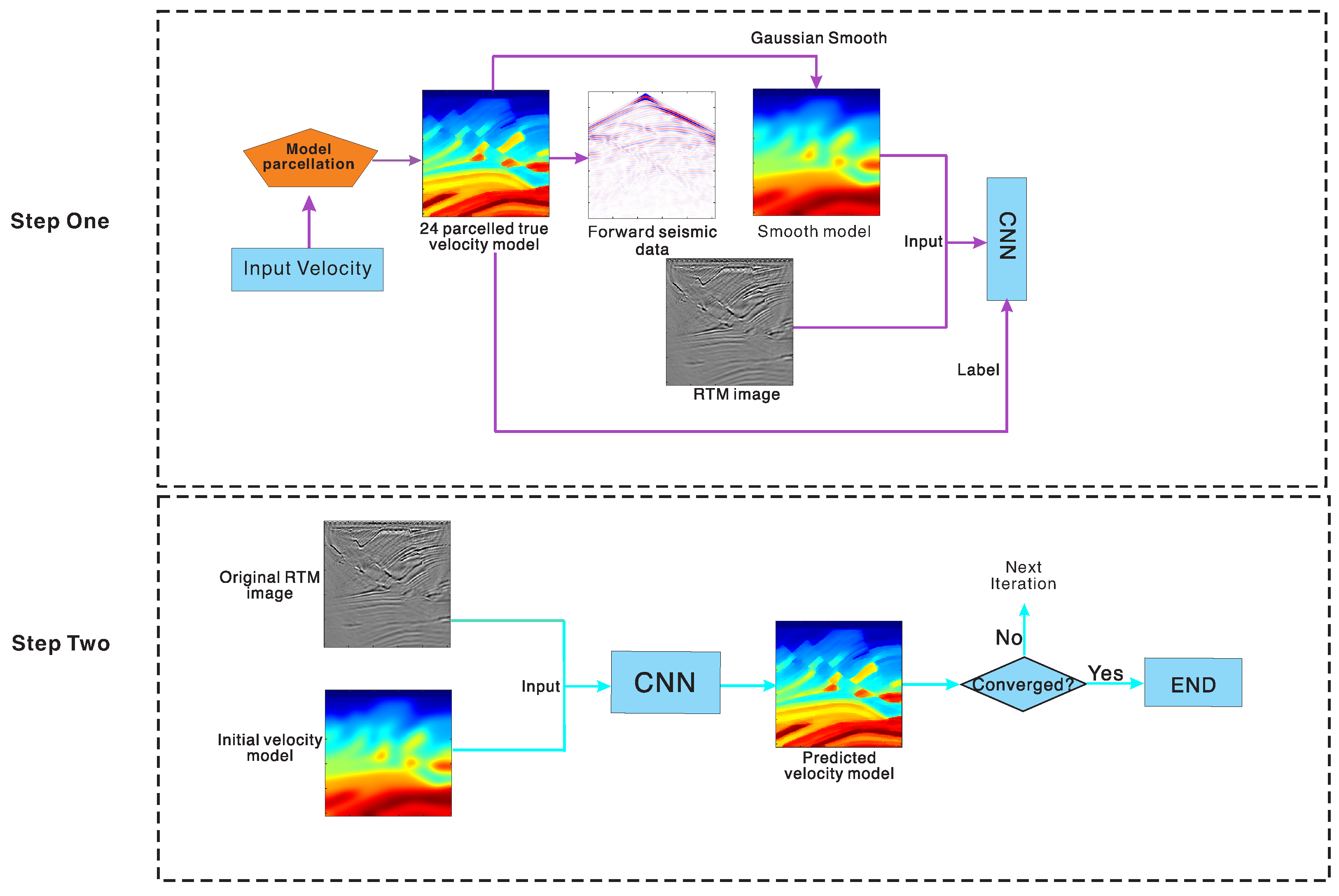
Figure 1 is a step-by-step iterative update pipeline of CNNVI. The two-loop structure represents a combination of network training and network prediction processes. Iterative updating refers to the use of network prediction results as the basis for the next iterative construction of the training set.
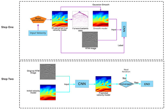
Figure 1.
The iterative step-by-step update structure. Step one denotes the training process, and step two denotes the prediction process. For the first iteration, the input velocity is the initial velocity model, and for the other iteration, it is the previous step’s prediction result.
Below, we will explain exactly how the iterative structure works. The CNNVI inversion has two parts, the network training process (step one) and the network prediction process (step two). The prediction of the network and the training of the next network are iterative processes that are continuously facilitated until convergence. Before proceeding with the CNNVI module, we constructed the input database for the network using angle RTM imaging and tomography. The input data containing the initial velocity model and migration image are used for the network prediction. It is worth noting that during the iterations of the CNNVI method, the input to the network prediction is always the original RTM image and the initial velocity.
The following paragraphs present a detailed description of the step-by-step iterative update pipeline. Step one denotes the training process, and step two denotes the prediction process. For the first iteration, the input velocity is the initial velocity model, and for the other iteration, it is the previous step two’s prediction result.
(a) Step one
Step one is the neural network training process. In CNNVI, the first step is to construct an appropriate training set. For the data-driven end-to-end approach to AI inversion, this typically involves generating a large batch of velocity samples that capture the full subsurface structure. To ensure optimal results, it is important to carefully consider the composition of this training set before starting the network training process. The subsurface is characterized by a plethora of intricate geological structures, including but not limited to salts, faults, folds, and unconformities, which have been formed by millions of years of evolution on Earth. Due to the remarkable diversity and complexity of these subsurface features, it remains a challenge to comprehensively capture them all using a training dataset of sufficient diversity.
We propose constructing a perturbed velocity model training set with similar characteristics to the initial model. Using the model parcelation method [22,33], we create some perturbed velocity models.
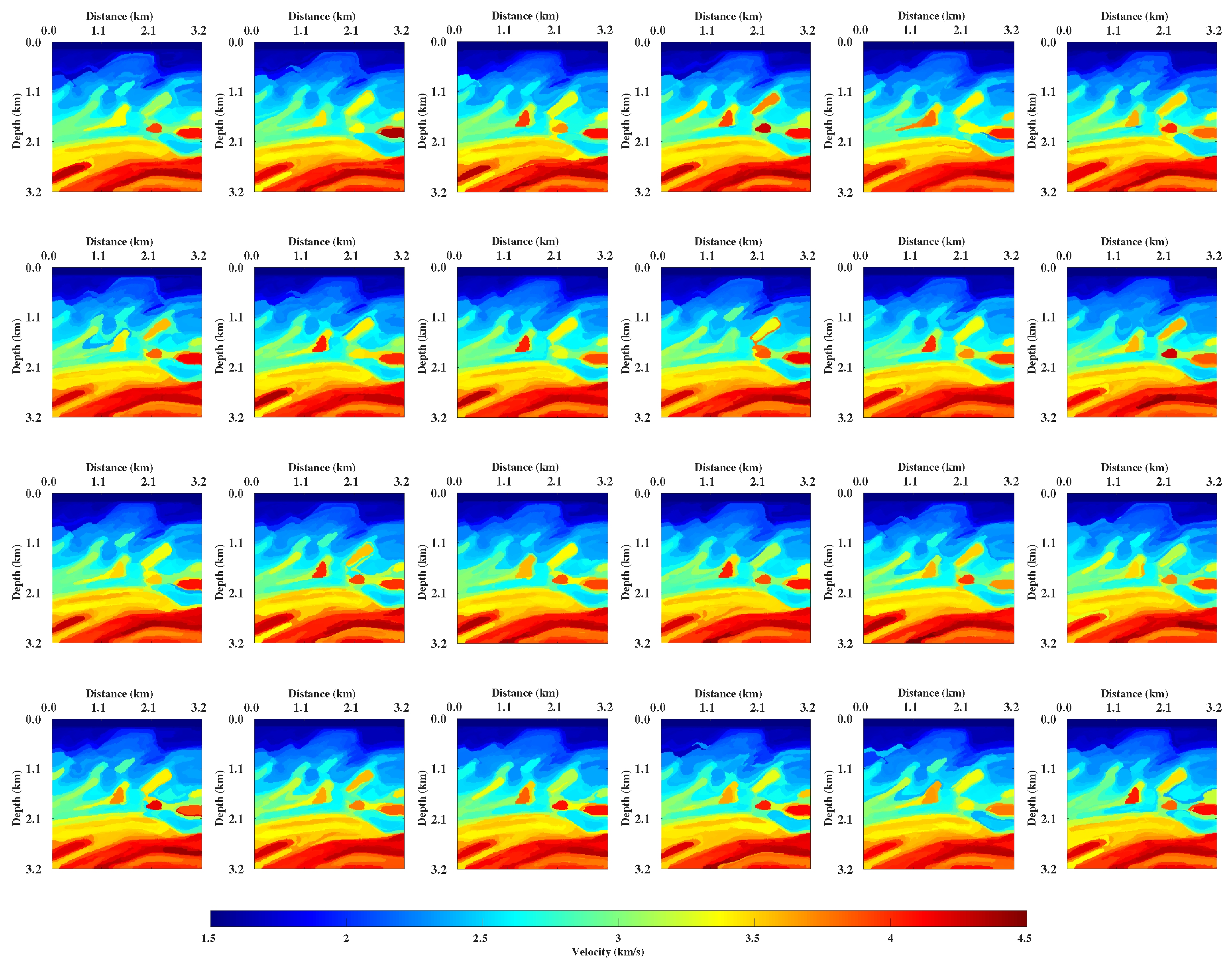
Displayed in Figure 2 is the 24-sample training set, which originates from the initial model utilizing the model parcelation approach in the first iteration. This technique introduces some reflection events to the training data. The parceled models, despite having similar features, exhibit distinct reflective interfaces and background velocity values in each iteration from the first to the final iteration. The model parcelation method enables the generation of a training library that possesses comparable features to the true velocity model. Subsequent model parcelation performed using a more improved initial model leads to a superior training database.
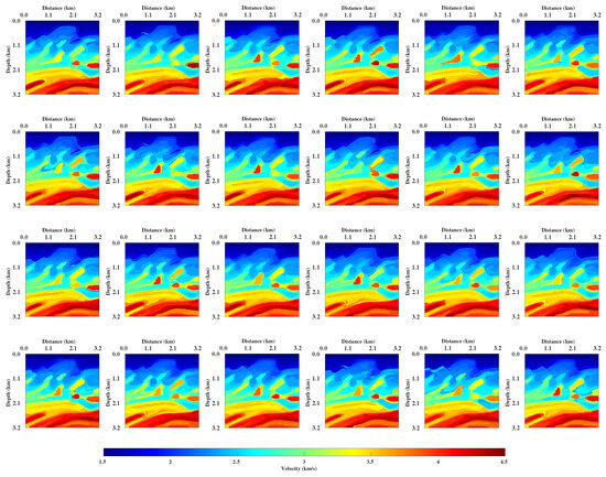
Figure 2.
Model parcelation diagram from the first iteration.
With the model parcelation method, we can obtain a perturbed model dataset for the first iteration of CNNVI training. We then construct samples from these parceled velocity models and use them as labels for network training. Through Gaussian smoothing and angle-domain RTM imaging, we obtain the initial velocity model and its corresponding migration components, which serve as the inputs for the first iteration of CNNVI. After the training of the neural network, we can obtain the parameters of a well-trained neural network. The initial iteration of the neural network training process in CNNVI is completed at this stage.
(b) Step two
The process shown by the sky blue line in Figure 1 is the neural network prediction process. As mentioned above, for the network prediction, we input the original initial model and RTM as a two-channel databody. It is worth noting that during the iterations of the CNNVI method, the input to the network prediction is always the original RTM image and the initial velocity model. The network prediction at the end determines whether the inversion converges or not. If it converges, the whole CNNVI process is ended. If it does not converge, model parcelation is performed on the new predicted velocity model to create the training dataset for the next iteration.
In addition, unlike the traditional CNN prediction process, we perform an error evaluation after the prediction. After the velocity model prediction, we can process forward modeling to obtain the corresponding synthetic data for error evaluation. Unlike classic FWI, which updates the velocity model depending on the residual data minimization, CNNVI only uses the data error to evaluate the predicted accuracy indirectly.
If it does not converge (the data error does not meet the convergence criteria, e.g., a threshold of the minimum data error), it continues model parcelation and the next inner-loop, forming an iterative process until convergence.
Here, we analyze the CNNVI step-by-step iterative process in detail. We always input the two-channel data including the original velocity model and migration image, so we have a fixed-input model space. At the end of one iteration, this better prediction is used for parceling to build the next training set. Thus, our training set space is progressively closer to the real subsurface medium space, and our prediction results are more accurate.
2.1.1. Physical Rationality Analysis
Under the Born approximation, we make the assumption that the updated model is composed of the initial model combined with a perturbation model .
where , k, and represent the model perturbation, iteration number, and step-length, respectively.
Based on its Taylor expansion, the derivative of an objective function is as follows [5]:
where and are the Taylor expansion’s higher-order term and the initial model, respectively. Ignoring , we obtain the following Equation (3):
Finally, the FWI iterative equation can be expressed as:
where g is the inversion gradient, and is the Hessian matrix. In traditional full-waveform inversion (FWI), the model parameters are updated iteratively using Equation (5). However, the seismic record for the initial model typically only contains first arrivals and a limited number of reflection signals. As a result, the gradient can be estimated by its migration image , as suggested by [2,34]. This allows us to simplify Equation (5) to the following form:
where is a complex function containing an inverse Hessian matrix [33]. In each iteration, the training process of the neural network aims to continuously adjust and optimize the fit of the complex function .
2.1.2. Angle-Domain RTM
Transitioning from single-frequency CNNVI to multi-scale CNNVI involves a significant increase in computational cost. To address this challenge, we propose incorporating angle-domain reverse time migration (RTM) [35] into CNNVI as a means of accelerating the convergence rate and enhancing the inversion process’s accuracy.
The zero-delay cross-correlation imaging condition is the most widely used RTM imaging condition and can be expressed as in Equation (7).
where t is the propagation time; x is the imaging point; and are the time- and space-domain wavefields, respectively; is the largest recording time; is the angle of our own choice; and is the imaging result. We can calculate the wavefield propagation direction by the Poynting vector method, which is expressed as follows:
where is the Poynting vector, is the velocity vector, and P is the pressure field. Calculating the Poynting vectors and of the source and detector wavefields, respectively, we can obtain the reflection angle by the following equation:
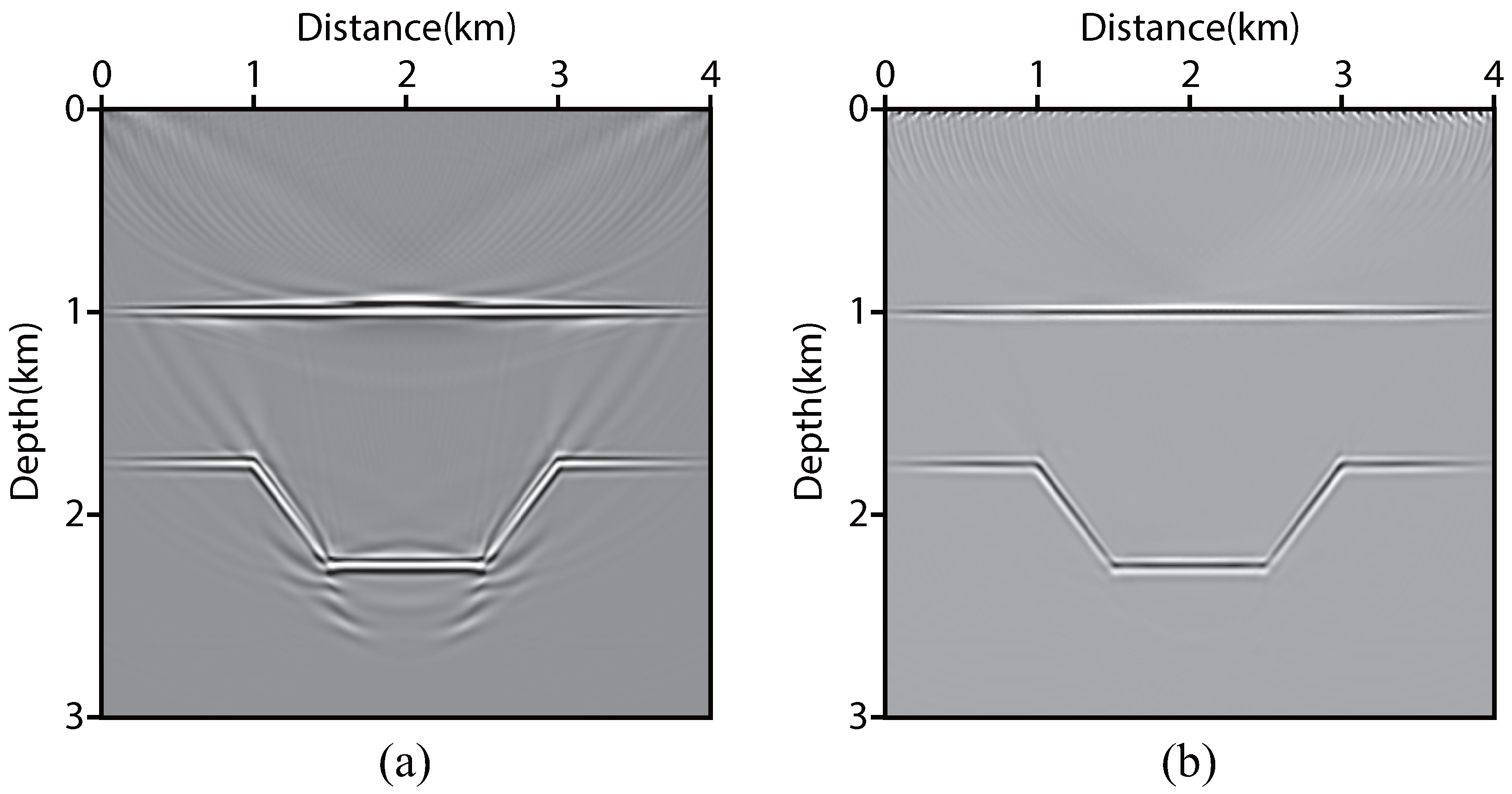
The purpose of the angle domain is to image seismic waves with specified reflection angles during the wavefield inter-correlation process of the RTM. It can effectively suppress wavefield noise and improve RTM imaging quality. Figure 3b shows the angle-domain RTM imaging result. It can be seen that the imaging result is much better than the normal RTM in (a). Thus, by introducing better RTM images into the neural network, the network prediction results can be improved. This allows us to enhance the RTM imaging results by angle-domain imaging conditions. Angle-domain RTM based on the Poynting vector method does not increase the computational effort, but it can accelerate the convergence speed of CNNVI.
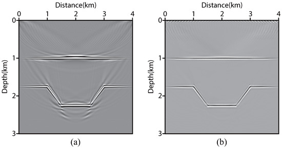
Figure 3.
The comparison of angle-domain RTM result with conventional RTM. (a) Conventional RTM imaging result. (b) Angle-domain RTM imaging result.
2.2. The Workflow of Multi-Scale CNN Velocity Inversion
In recent years, Fu et al. [27], Choi and Alkhalifah [28], Qu et al. [29], Guo et al. [30], and Liu et al. [31] further developed the MS strategy based on the research of Bunks and achieved good inversion results in its application to FWI.
Multi-scale full-waveform inversion is a cutting-edge technique that addresses two key challenges in seismic inversion. Firstly, it mitigates the uncertainty associated with high-frequency components, which can introduce errors and redundancy in the inversion process. Secondly, we first invert the background velocity using low-frequency information and then gradually reconstruct fine-scale details using high-frequency information. Similar to FWI, neural network inversion is also a highly nonlinear inverse problem. By combining these approaches, the same multi-scale algorithm can be used to integrate AI inversion and optimize the inversion process.
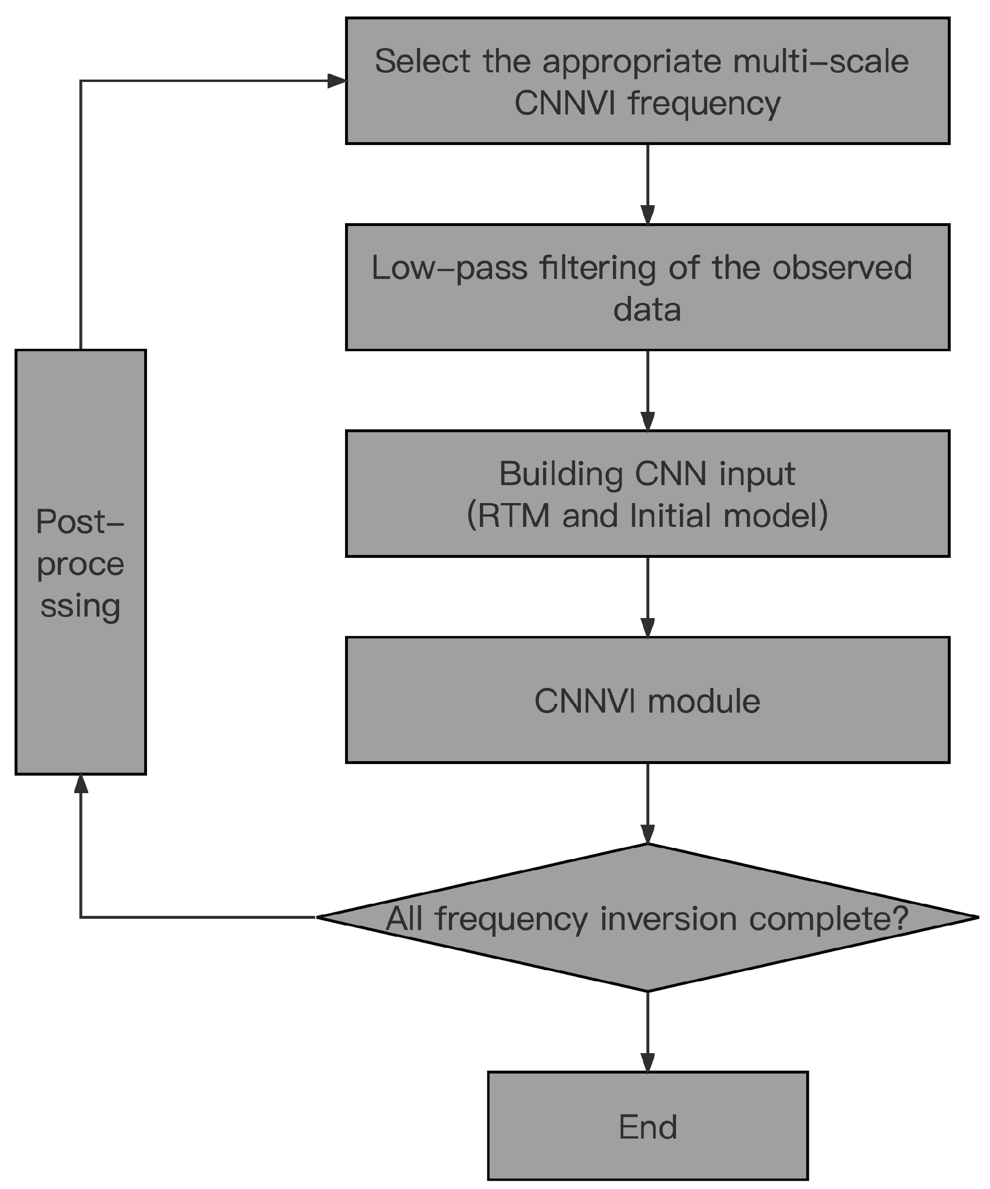
Figure 4 is the workflow of the Ms-CNNVI method. The process of the Ms-CNNVI method is divided into the following parts:
- To begin, we carefully choose several inversion frequencies at various scales, taking into account the specific features of the observed seismic data. In a given area, for example, our selection may begin at 5 Hz and progress to 10 Hz, 15 Hz, and 20 Hz in a sequential manner to perform the inversion. Then, at the beginning of the iteration we start with the inversion at low frequencies.
- Once we have chosen the inversion frequency for the current iteration, it is time to apply a low-pass filter to the observations. This step ensures that the data are properly prepared for downstream processing.
- In the construction of the CNN input, both the RTM and the initial velocity model play crucial roles. The RTM component is obtained through the technique of angle-domain RTM imaging, and the initial velocity model can be obtained via tomography imaging or migration velocity analysis (MVA).
- CNNVI is performed using the input data obtained in step c, and more accurate inversion results are obtained. The specific principles of the CNNVI module were introduced in the previous subsection.
- The inversion process is complete for all selected frequencies. If complete, the entire Ms-CNNVI process is ended; if not complete, the post-processing of the data continues.
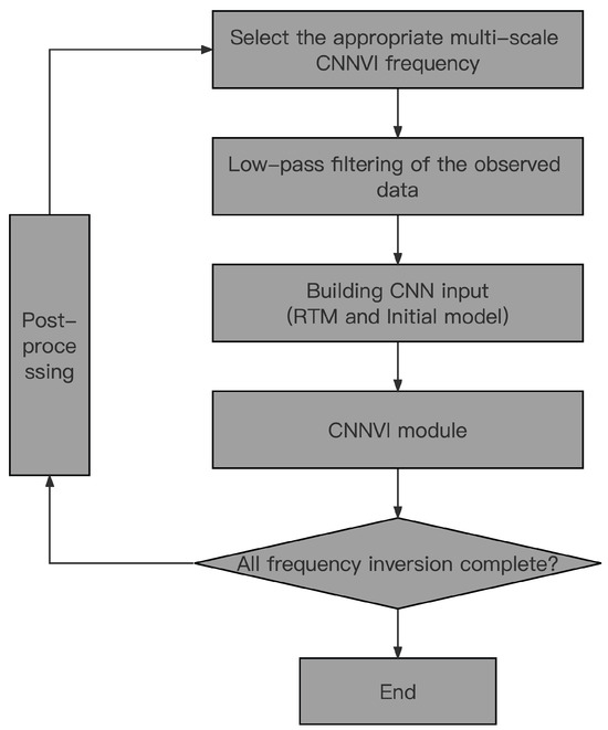
Figure 4.
The workflow of the Ms-CNNVI method.
Figure 4.
The workflow of the Ms-CNNVI method.
The MS strategy can reduce the errors introduced in the data fitting process and obtain better gradient information, thus improving the inversion accuracy. We first invert the background velocity using low-frequency information and then gradually reconstruct the fine-scale details using high-frequency information. As for CNNVI, the initial velocity model and its corresponding initial RTM image are always used as input to the network for inversion. The FWI gradient can be approximated by the migration image of the initial model [2,34]. Thus, multi-scale inversion can reduce the error in the gradient, producing a more accurate migration component, and thus improve the accuracy of the whole inversion.
Based on Equation (6), the multi-scale inversion equation for different frequencies can be expressed in the following form:
where , , represents the CNN mapping, and is the inversion frequency.
Algorithm 1 is the pseudocode of the Ms-CNNVI method.
| Algorithm 1 Multi-scale CNNVI. |
| Given Inversion frequency Observed seismic data Initial velocity model Initialize , Select the max inversion frequency
|
2.3. Method Details
2.3.1. The Structure of the Network in CNNVI
In this paper, we use an attention U-Net to introduce some attention layers into a standard U-Net. We can improve the network’s attention to structures such as faults and layers based on the attention layers, thus improving the accuracy of the inversion of subsurface structures. Figure 5 shows the structure the attention U-Net in this paper. The specific structure of the network was described in our previous paper [36].
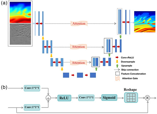
Figure 5.
The structure of the attention U-Net in this paper. (a) A standard U-Net with some attention gates. (b) The inner structure of an attention gate.
The attention U-Net is a potent neural network comprising diverse elements, encompassing downsampling and upsampling strata, skip connections, and attention strata. The encoder segment of the network is fashioned using Conv, ReLU, and downsampling strata. The encoder and decoder segments of the network share an asymmetrical structure. Additionally, the attention strata augment the precision of the network by concentrating on the most informative attributes throughout the training procedure.
The attention U-Net is a powerful neural network that consists of various components, including downsampling and upsampling layers, skip connections, and attention layers. The encoder part of the network is constructed using Conv, ReLU, and downsampling layers, where Maxpooling is used as the downsampling layer. The encoder and decoder parts of the network have an asymmetric structure in common. Furthermore, the attention layers enhance the accuracy of the network by focusing on the most informative features during the training process. Overall, the attention U-Net is a powerful tool that can be used in various applications, including image segmentation and classification, due to its ability to extract and utilize important features from the input data. In this paper, we choose an attention U-Net as the basic structure of CNNVI, which can greatly improve the inversion accuracy.
2.3.2. The Data Processing and Training Details
By paying close attention to data pre-processing, deep learning models can achieve better performance and accuracy, leading to improved predictions. Across the whole Ms-CNNVI process, there are some data processing elements worth highlighting. Initially, it is imperative to implement deep illumination compensation and Laplace filtering on the data post-RTM imaging. The purpose of Laplace filtering is to eradicate low-frequency noise. Furthermore, deep illumination compensation for RTM endeavors to enhance the network’s inversion on deep background velocity and reflectivity.
Additionally, as illustrated in Equation (10), it is necessary to perform post-processing on the output predicted velocity model following each CNNVI in order to obtain the initial velocity model for the subsequent multi-scale frequency inversion. The post-processing depicted in Figure 4 entails a limited number of Gaussian smoothing procedures applied to the prediction model of CNNVI. This is due to the fact that in CNNVI, our training involves mapping from smoothed data to the accurate model, and the input in the prediction process impacts the output result of the network if it contains data with numerous sharp structures. Therefore, a small amount of smoothing is administered to the velocity model, aligning it more closely with the characteristics of the network model trained in each CNNVI.
The epoch, learning rate, batch size, and activate function of every iteration are 800, 0.001, 1, and Tanh, respectively.
3. Numerical Results
In the section dedicated to numerical results, we present the practical experiments carried out to validate the Ms-CNNVI method. Initially, we conducted an ablation experiment to evaluate the effectiveness of our proposed multi-scale (MS) strategy within the Ms-CNNVI method. Following this, we applied the Ms-CNNVI method to complex models and compared it with multi-scale FWI. Finally, we illustrate how to implement Ms-CNNVI using an inaccurate initial velocity model.
The parameters of the forward modeling algorithm in the RTM for constructing the training set and the FWI for testing in this paper were as follows. We utilized the Ricker wavelet as the wavelet function. The number of sources was 25, the spatial sampling interval was 12.5 m, the time sampling interval was 0.001 s, and the travel time was 4 s. Two hundred and fifty-six receivers were evenly distributed on the surface.
3.1. Ablation Experiments with Ms-CNNVI Method
We first tested the effectiveness of the Ms-CNNVI method proposed in this paper based on the Sigsbee velocity model. In this paper, we propose an MS convolutional neural network (CNN) velocity inversion (Ms-CNNVI) method. Specifically, it includes the following contributions.
Firstly, we propose an MS AI inversion strategy. Secondly, in the multi-scale AI inversion process, we propose to incorporate a smoothing strategy. Finally, we introduce angle-domain RTM in each CNNVI module. Compared to conventional CNNVI, this paper makes three improvements. Thus, we performed ablation experiments to test the influences of different modifications on the inversion results.
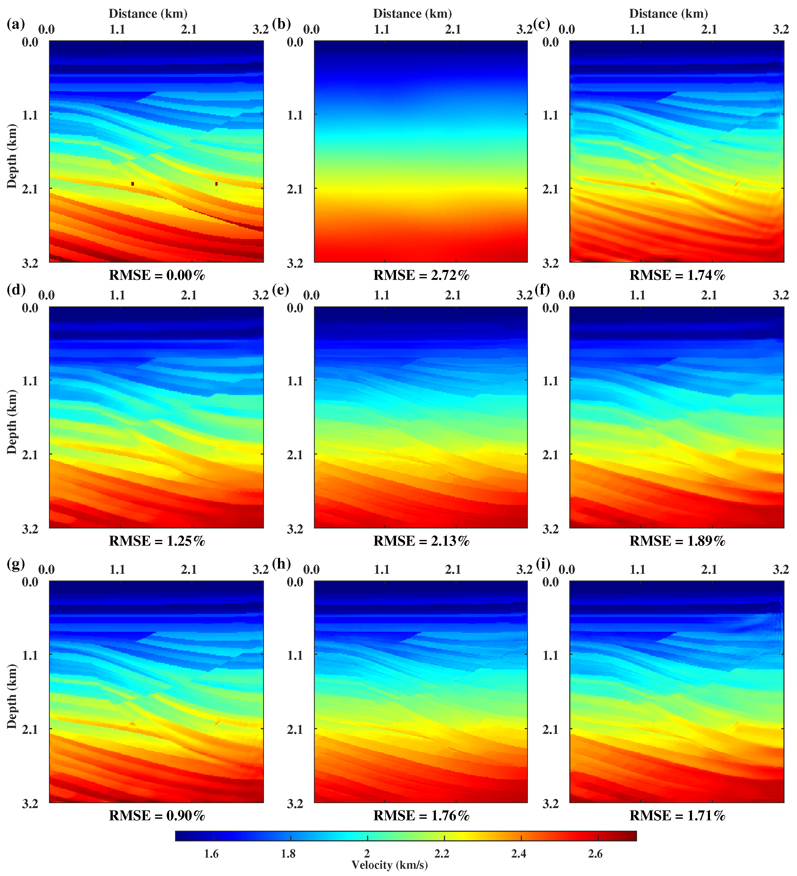
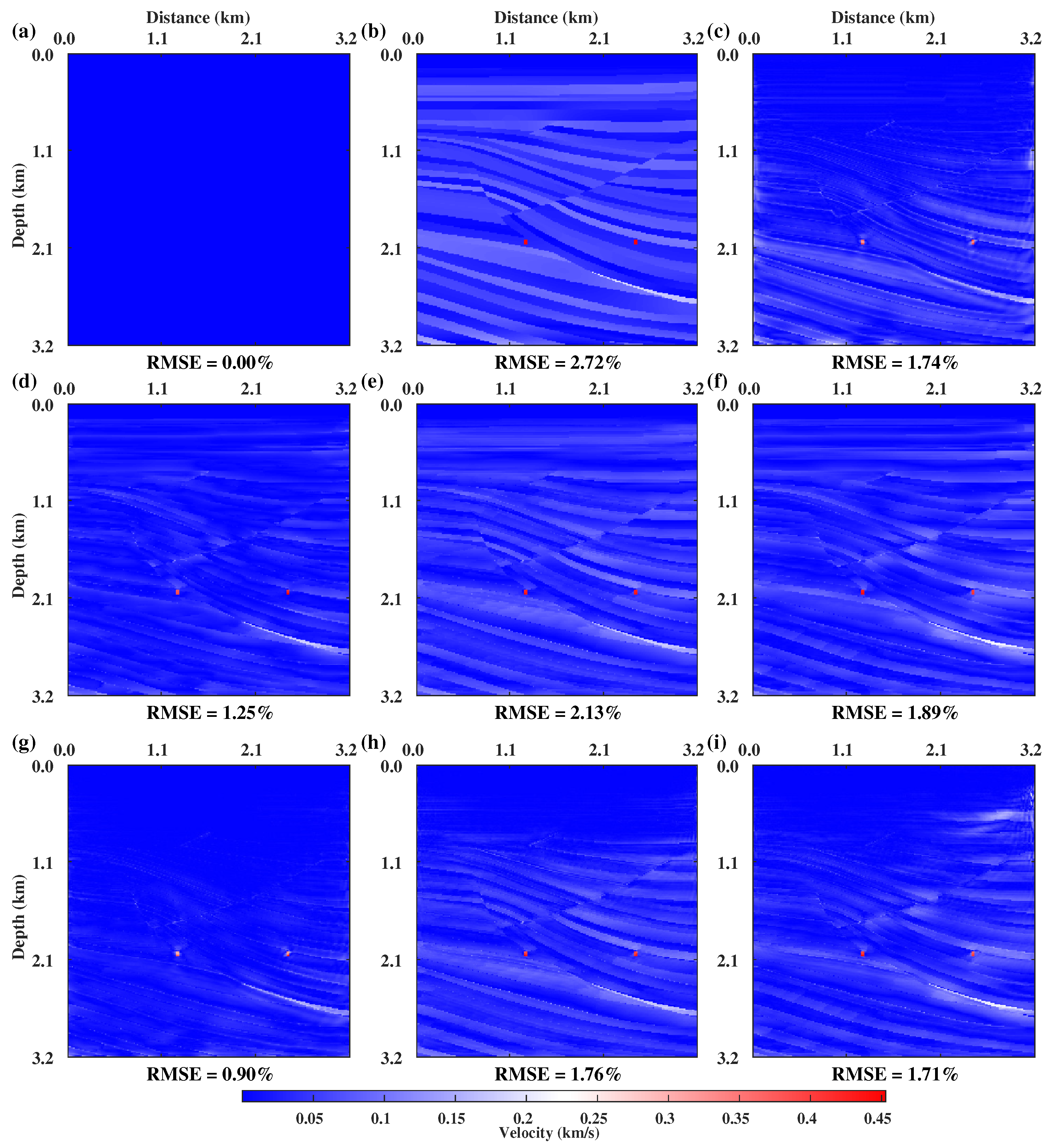
Figure 6 depicts the ablation experiments conducted with Ms-CNNVI using the Sigsbee model. To assess the method’s capability of updating the deeper section of the velocity model, we chose to establish a 1:1 aspect ratio for the model’s ordinate. (a) and (b) represent the true and initial velocity models, respectively. (c) portrays the inversion result based on traditional multi-scale FWI. (d) and (g) show the inversion results obtained through the proposed Ms-CNNVI and its corresponding FWI. (e) and (h) exhibit the inversion results solely based on CNNVI and its corresponding FWI. Finally, (f) and (i) demonstrate the CNNVI results exclusively derived from our proposed smoothing strategy and its corresponding FWI.
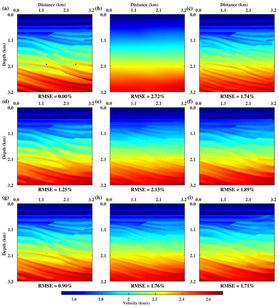
Figure 6.
The ablation experiments with Ms-CNNVI based on Sigsbee model. (a) True Sigsbee velocity model. (b) Original velocity model. (c) The inversion result based on Ms-FWI. (d,g) The inversion results based on the proposed Ms-CNNVI method and its corresponding FWI. (e,h) The inversion results based only on the CNNVI method and its corresponding FWI. (f,i) The inversion results based only on our proposed smoothing strategy and its corresponding FWI.
It is worth noting that Figure 6e is the result obtained using CNNVI based on 21 Hz migration images, and Figure 6f is the result of adding a smoothing strategy to the 21 Hz CNNVI consistent with that in the multi-scale process.
By comparing Ms-CNNVI with conventional FWI in Figure 6, we can find that the RMSE of Ms-CNNVI was much smaller than that of conventional FWI. In addition, the conventional FWI method could reconstruct well for the shallow layers (<1.5 km), but the velocity reconstruction in the deep part was not good. However, for the Ms-CNNVI method, the deep background velocity and structural features could be accurately reconstructed.
Comparing (e) with (d) in Figure 6, we find that the MS-CNNVI method’s inversion results were far better than those of the single CNNVI at any depth position in terms of background velocity and geological structure. Comparing (e) with (f), we find that using only the smoothing strategy could improve the inversion effect. In contrast, multiple scales from low-frequency to high-frequency inversion could significantly enhance the inversion accuracy. Through the ablation experiments, we demonstrated that both the multi-scale and smoothing strategies could improve the inversion effect, but the multi-scale strategy was more critical. By comparing (g), (h), and (i), we find that the inversion effect could be further improved by using conventional FWI based on the AI inversion results.
In the RTM and FWI processes, the forward modeling constitutes the most time-consuming aspect. Meanwhile, the remaining computational procedures are negligible. Running environments and code languages may produce varying running times. Thus, to evaluate the efficiency of the two methods, we compared their respective forward modeling counts.
The comparison of the residual between the velocity models shown in Figure 6 and the true velocity model is depicted in Figure 7. Fewer residual structures in the residuals represent a better inversion effect. We found that the residuals of the FWI results had minor residual information in the shallow part, which proves that FWI is effective for shallow inversion. The Ms-CNNVI method presented in this paper had even fewer residual structural details in the deep central part. This proves that our method can invert the background velocity and geological structure information in the deep part very well. The residuals of Figure 7g were minimal at any depth, which proves that our Ms-CNNVI combined with FWI can achieve higher-accuracy inversion.
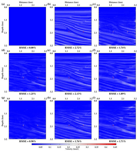
Figure 7.
Residuals of the inversion results with the real model. (a) True Sigsbee velocity model’s residual. (b) Original velocity model’s residual. (c) The inversion result’s residual based on Ms-FWI. (d,g) The inversion results’ residuals based on the proposed Ms-CNNVI method and its corresponding FWI. (e,h) The inversion results’ residuals based only on the CNNVI method and its corresponding FWI. (f,i) The inversion results’ residuals based only on our proposed smoothing strategy and its corresponding FWI.
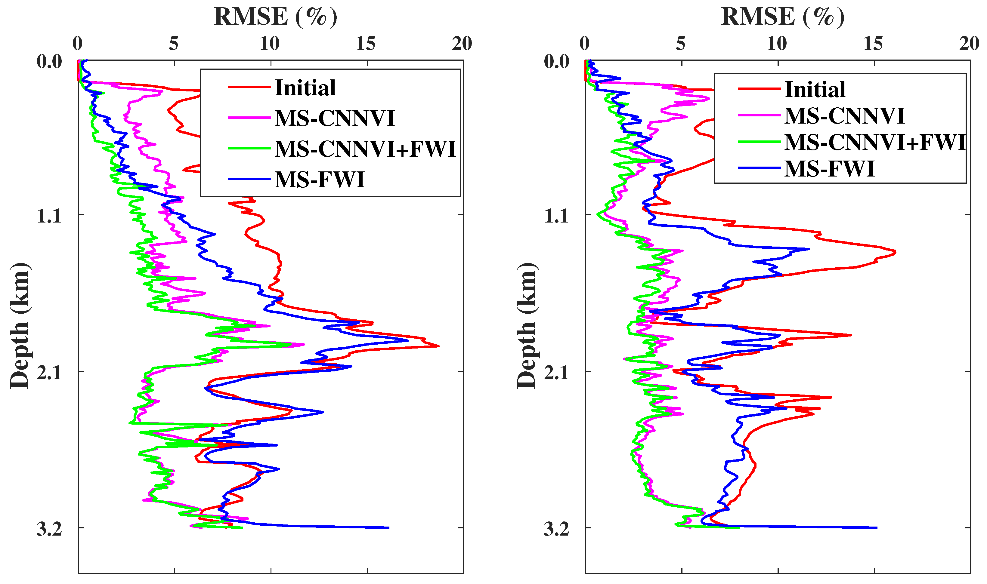
Figure 8a shows the cumulated RMS errors for each position in the same layer, and (b) shows the single trace velocity extracted from Figure 6. The solid lines represent the results of AI inversion, and the dashed lines are the corresponding FWI results. A smaller RMSE means better inversion for that layer. We can find that the error of FWI in the shallow layers was low, proving that FWI has a good inversion effect for shallow layers. The results of the Ms-CNNVI method and its corresponding FWI proposed in this paper had the lowest error, proving the effectiveness of the proposed method. The single-channel comparison showed that the results obtained by the Ms-CNNVI method were closest to the real velocity model.
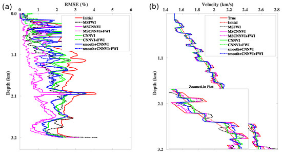
Figure 8.
(a) The cumulated RMS errors for each position in the same layer. (b) Comparison of the single trace velocity extracted from Figure 6.
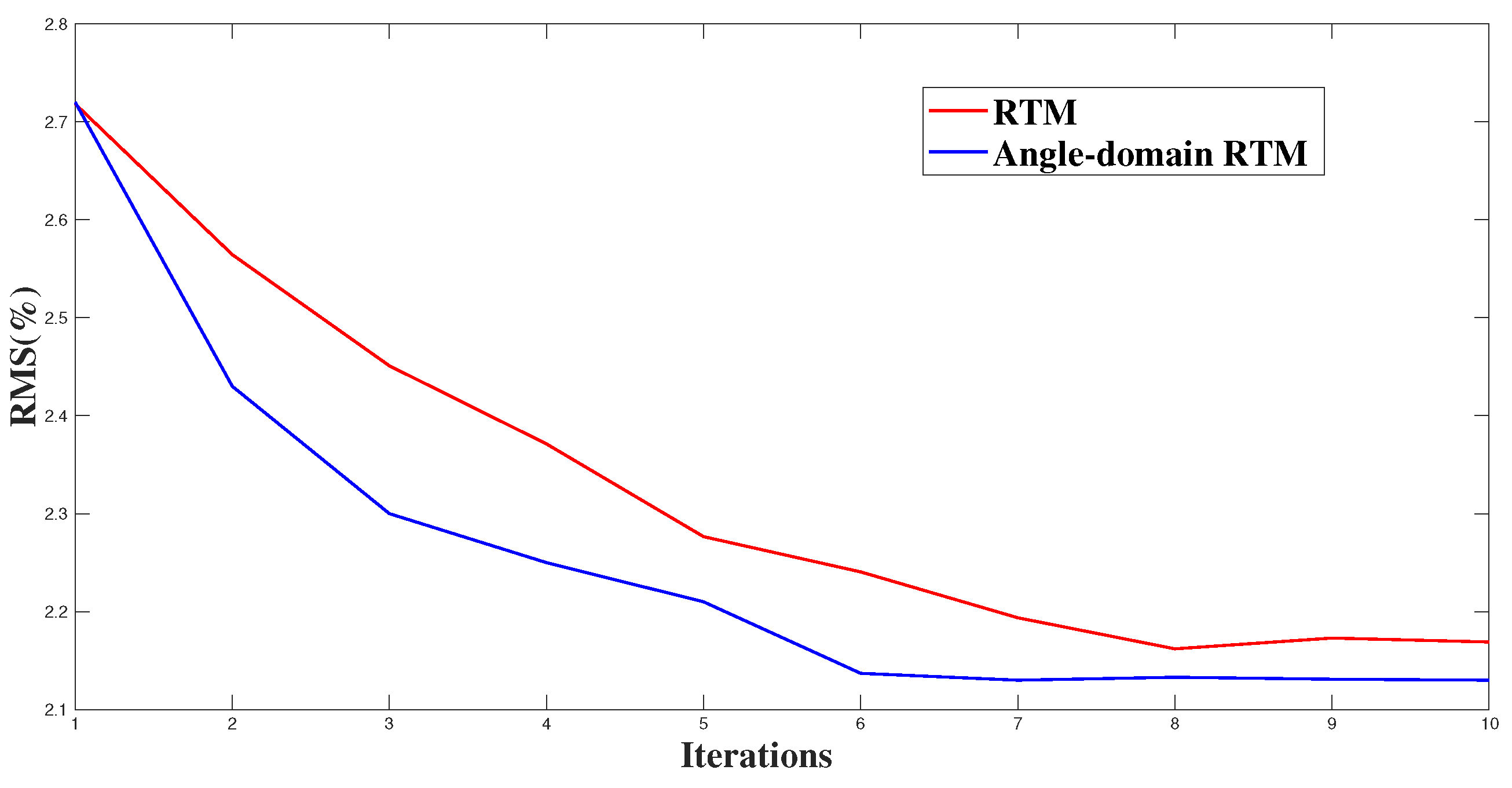
For a single CNNVI, Figure 9 shows the change in RMS as the number of iterations increased for both RTM methods. We can find that angle-domain RTM accelerated the convergence speed of CNNVI. In addition, the introduction of angle-domain RTM could slightly improve the inversion effect of CNNVI. This also demonstrates the utility of the third contribution of this paper.
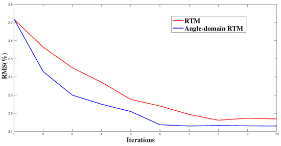
Figure 9.
The variation of RMS with the number of iterations for the two RTM methods in a single CNNVI.
The Ms-CNNVI method converged at the sixth iteration, as Figure 9 shows. For each iteration, 24 RTMs of the model were required, where each RTM contained two wavefield propagations. The total number of iterations was 24 × 2 × 6 = 288. For FWI, three wavefield propagations were required per iteration for a total of 150–250 iterations. Thus, the total number of wavefield propagations for FWI was 450–750, which is much more than for our method.
3.2. Complex Velocity Model Testing
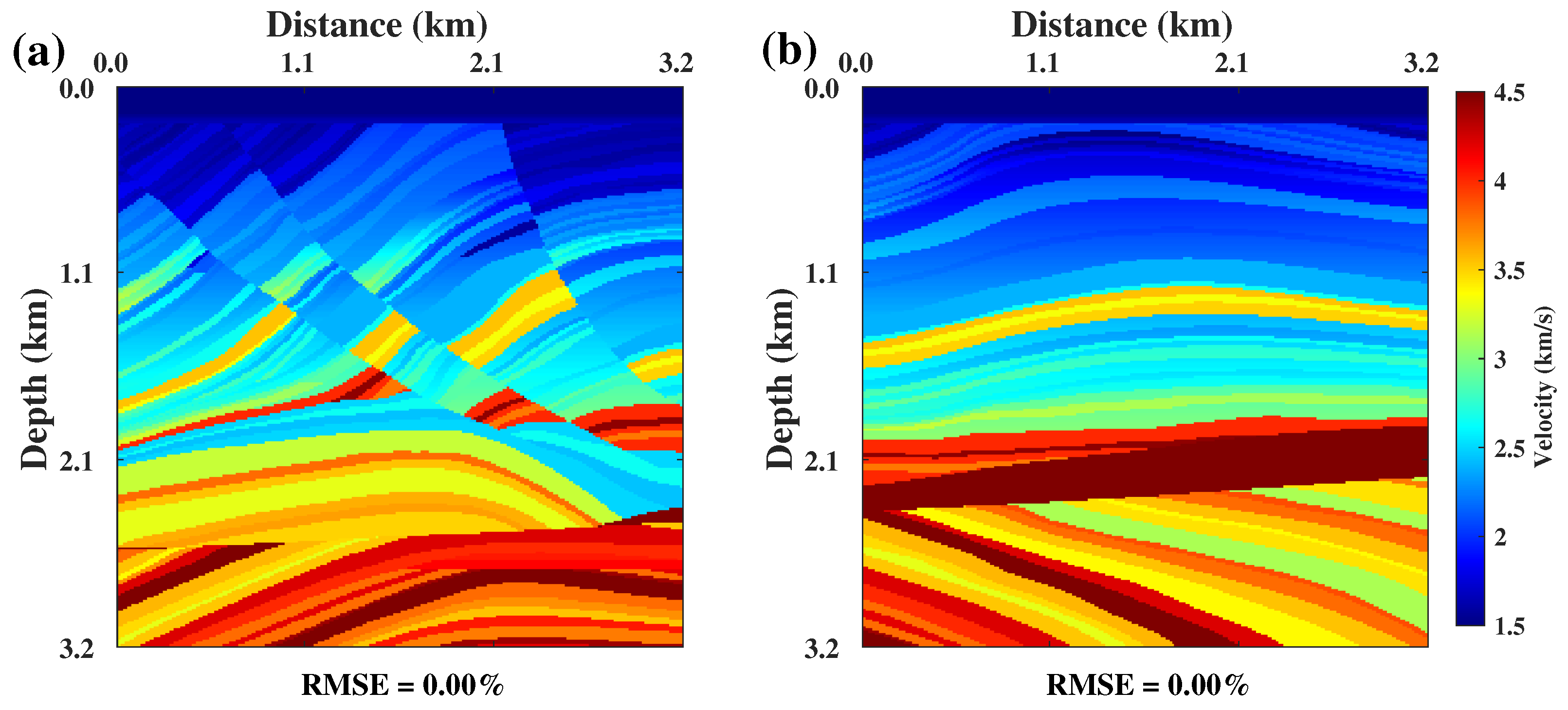
Then, we tested the method in a complex model. Figure 10 shows the two true velocity models intercepted from the Marmousi model.
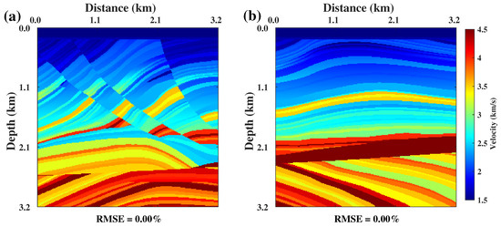
Figure 10.
Two true velocity models intercepted from the Marmousi model. (a) Interception of the left part in the Marmousi model. (b) Interception of the right part in the Marmousi model.
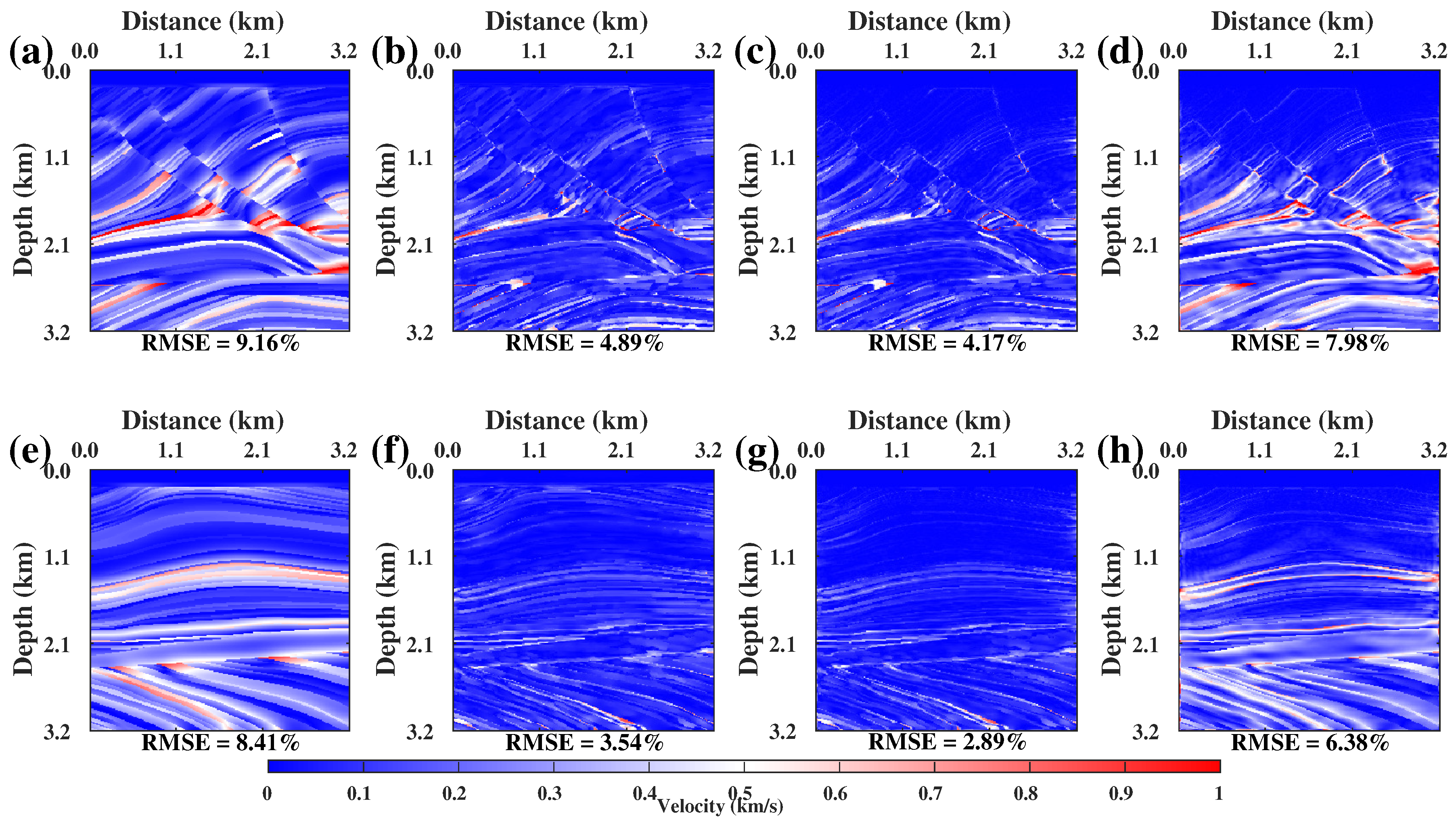
Figure 11a,e show the original model. (b) and (f) are the Ms-CNNVI results. (c) and (g) are the FWI results with (b) and (f) as the original models. (d) and (h) are the multi-scale FWI results with (a) and (e) as the original models. Our Ms-CNNVI method achieved impressive inversion results, even in complex models. Our findings reveal that the RMSE results obtained from our Ms-CNNVI approach were considerably lower than those of multi-scale FWI. Notably, the most significant aspect of our method was its ability to outperform conventional multi-scale FWI in the deeper layers, accurately reconstructing geological structures, such as the boundary of the high-velocity body. Moreover, our Ms-CNNVI approach demonstrated superior performance in recovering the deeper part’s background velocity, an area in which the conventional FWI results proved particularly inaccurate. In light of these findings, we took the output result of Ms-CNNVI as the initial model, leading to further error convergence. Figure 12 shows the residuals of the inversion results with the real model. We can find that the residuals of Ms-CNNVI+FWI had the least useful signal information remaining, which means that its inversion results were the best.
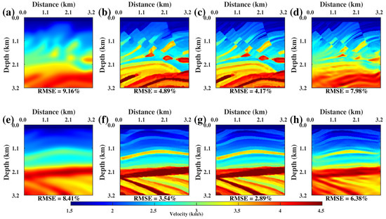
Figure 11.
(a,e) The original model. (b,f) The Ms-CNNVI results. (c,g) The FWI results with (b,f) as the original models. (d,h) The multi-scale FWI results with (a,e) as the original models.
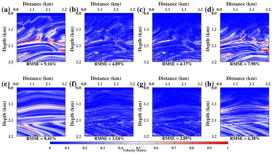
Figure 12.
Residuals of the inversion results with the real model. (a,e) The original models’ residuals. (b,f) The Ms-CNNVI results’s residuals. (c,g) The FWI results’s residuals with (b,f) as the original models. (d,h) The multi-scale FWI results’ residuals with (a,e) as the original models.
The comparison shown in Figure 13 provides a quantitative assessment of the inversion results for each depth by measuring the RMSE across all positions. The order of the lines in the graph represents the different models: initial model, Ms-CNNVI, Ms-CNNVI+FWI, and FWI, represented by blue, magenta, green, and blue lines, respectively. The RMSE of the AI-based method was lower than that of the FWI method at any depth. FWI has good inversion for shallow layers, but the accuracy of inversion for deep layers is poor. The method proposed in this paper can solve this problem very well.
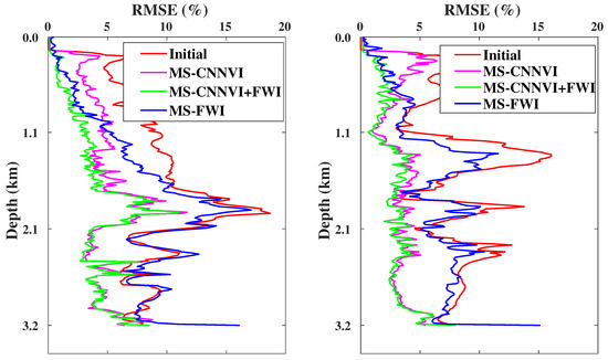
Figure 13.
The cumulated RMS errors for each position in the same layer.
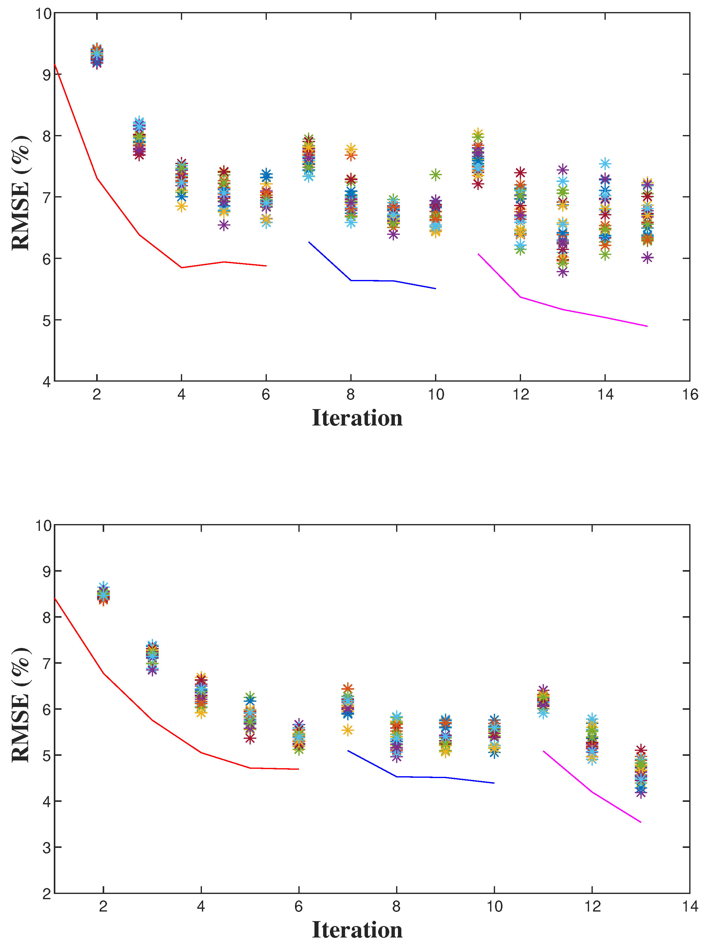
Figure 14 shows the RMSE of the Ms-CNNVI results with the number of iterations. The red, blue, and magenta lines represent the 7 Hz, 14 Hz, and 21 Hz CNNVI, respectively. The scatter represents the RMS error of the different training models obtained after model parcelation. After the inversion from low to high frequencies, the error underwent a continuous decreasing process three times. Furthermore, comparing the red line to the blue line and the blue line to the magenta line shows a rise in the error caused by the smoothing strategy we added. Although the smoothing strategy caused a slight rise in the error, it decreased rapidly in the next few iterations.
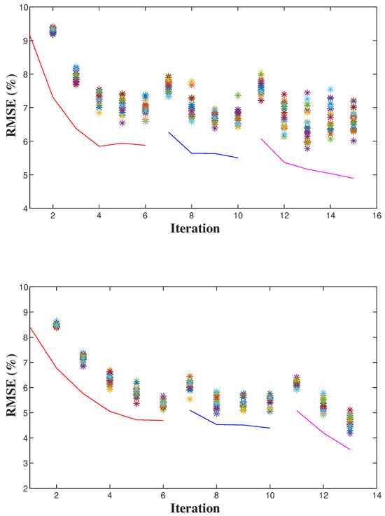
Figure 14.
The RMS errors of the Ms-CNNVI results with the number of iterations. The red, blue, and magenta lines represent the 7 Hz, 14 Hz, and 21 Hz CNNVI, respectively. The scatter represents the RMS error of the different training models obtained after model parcelation.
One interesting phenomenon deserves attention. According to the scatters, the error in the dataset used for training decreased with each iteration and was greater than the error in the network prediction. We used the training set shown in the scatters for network training and prediction to obtain more accurate prediction results. Then, the training set was reconstructed with this prediction model to obtain more accurate results for the next iteration. The process of continuously building more accurate training sets is also the core of the proposed method.
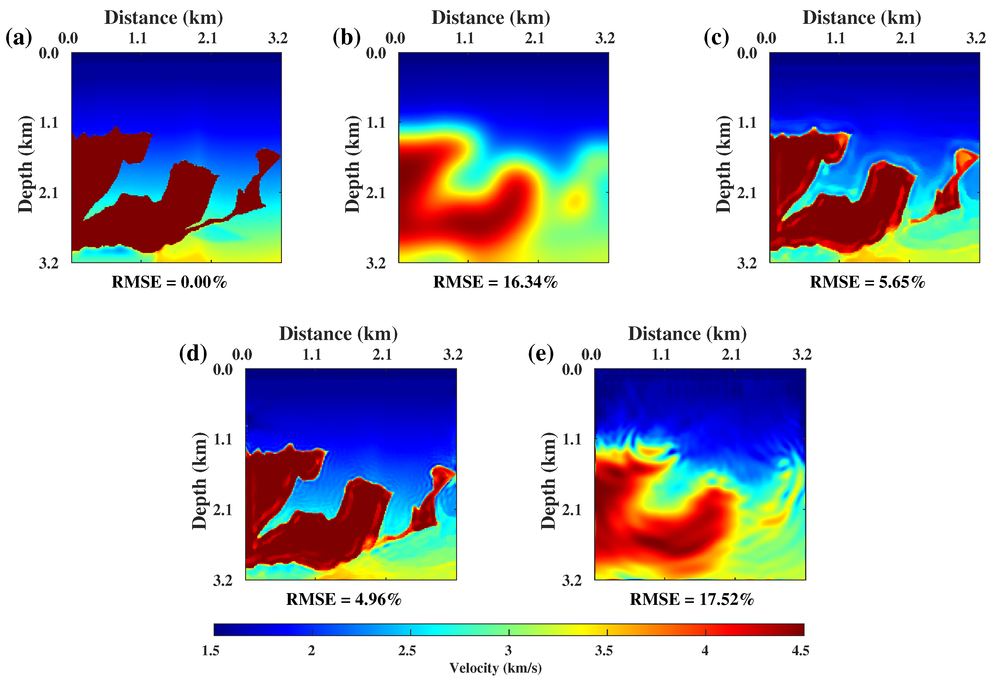
Next, we tested the effectiveness of this paper’s method in a salt model. We selected a salt model with a highly complex structure, the inversion of which is very challenging. Figure 15a,b show the true model and initial model, respectively. (c) is the inversion result of Ms-CNNVI. (d) and (e) are the multi-scale FWI results with (c) and (b) as the original models. We can find that this paper’s method carved the salt domes’ boundary features very well. The velocity structure below the salt dome was also well recovered.

Figure 15.
(a,b) The true model and initial model. (c) The inversion result of Ms-CNNVI. (d,e) The multi-scale FWI results with (c,b) as the original models.
3.3. Ms-CNNVI from a Bad Initial Velocity Model
After verifying the previous two cases, we demonstrate that the method in this paper has higher accuracy than FWI, especially for deep inversion. Moreover, traditional FWI relies more on the initial model. For a poor initial model, the gap between the data obtained by modeling the initial model and the observed data is too large, directly leading to the nonconvergence of the inversion. The Ms-CNNVI method in this paper also relies on the initial model. For FWI, in the case of a poor initial model, we can usually recover the background velocity first by methods such as tomography or full travel-time inversion [37] before further proceeding with a more accurate FWI. Then, the same strategy can be used for our Ms-CNNVI to construct the initial model containing more accurate background velocity.
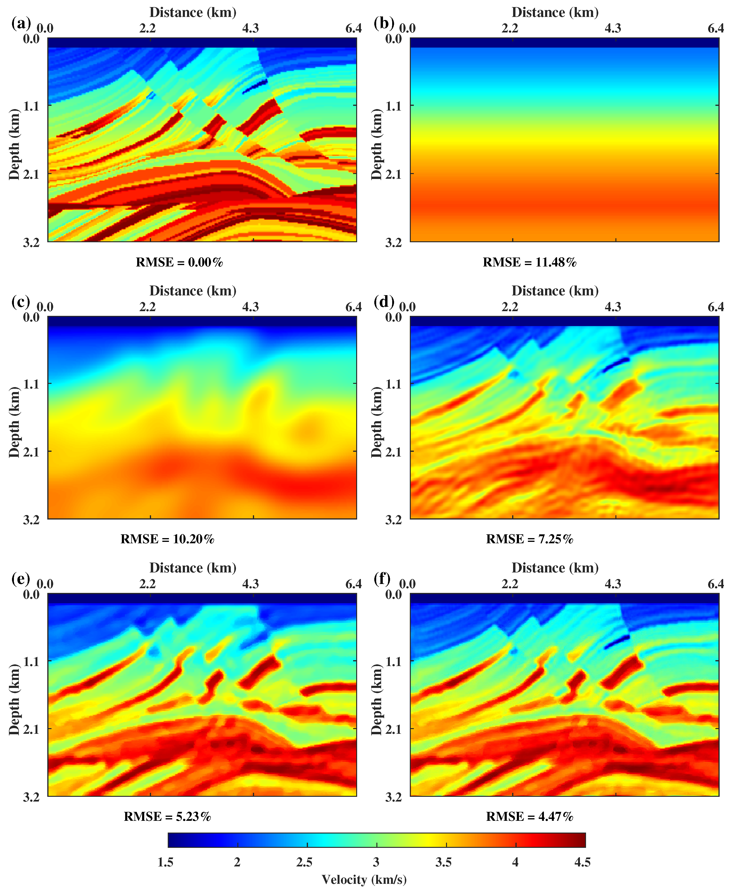
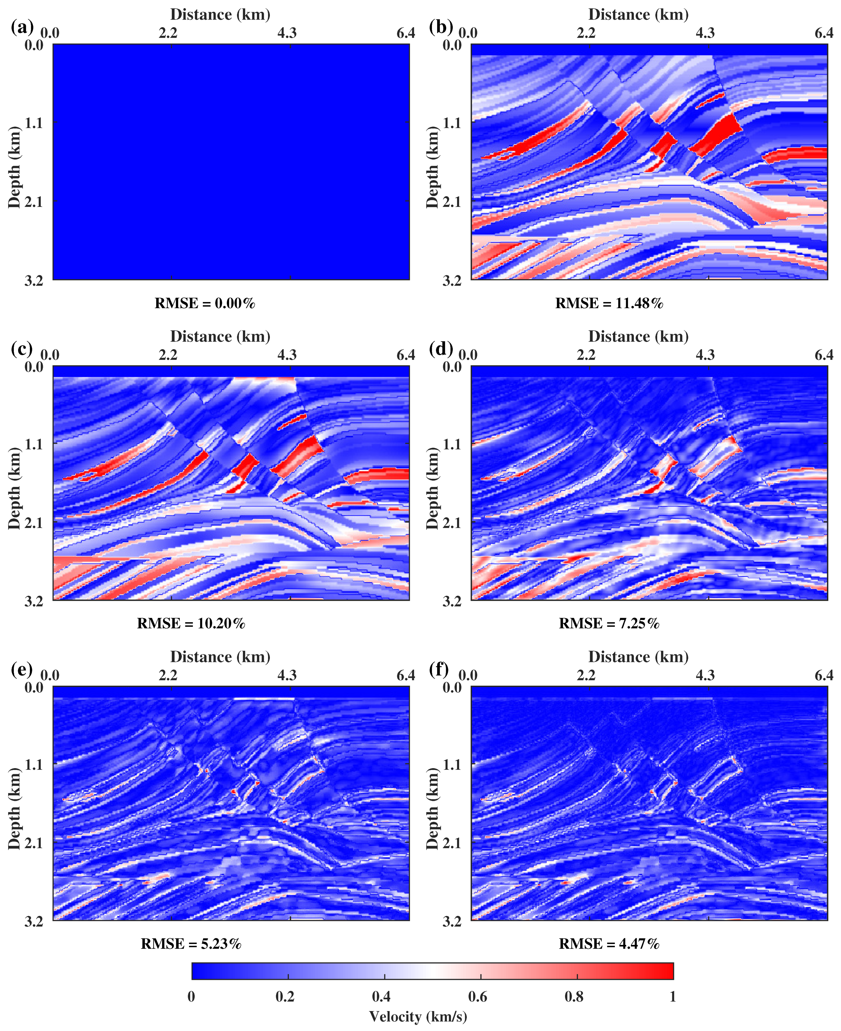
Figure 16b shows a poor initial velocity model. In this study, we firstly reconstructed the background velocity by FTI, as (c) shows. Figure 16d shows the inversion result with FTI (c) as the initial model. The FWI method effectively reconstructed the background velocity information, as Figure 16d shows. However, we also observed that the velocity information of the deeper parts was not as well reconstructed. At this point, the FWI method reached convergence. Continued iterative inversion did not produce better results.
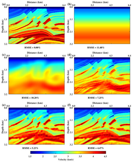
Figure 16.
(a) The true model. (b) The initial model. (c) The FTI result with (b) as the initial model. (d) The FWI result with (c) as the initial model. (e) The Ms-CNNVI method inversion result with (c) as the initial model. (f) The FWI result with (e) as the initial model.
Figure 16e displays the inversion result of Ms-CNNVI with FTI (c) as the initial model, where the RMSE decreased significantly. We found that the result obtained by the Ms-CNNVI method was better than the FWI result for both background velocity and structural features. This proves that the error can be further converged using the AI method based on FWI. In particular, the information on deep folds and high-velocity bodies was better portrayed. This also proves that our proposed scheme of constructing the background velocity and continuing the accurate inversion by AI is feasible. Finally, we continued to use FWI on the inversion result of Ms-CNNVI (e), which could provide a higher-accuracy velocity model.
Figure 17 shows the residuals of the inversion results with the real model. We also found that the residuals of Figure 17f had the least useful signal information remaining, which meant that these inversion results were the best.
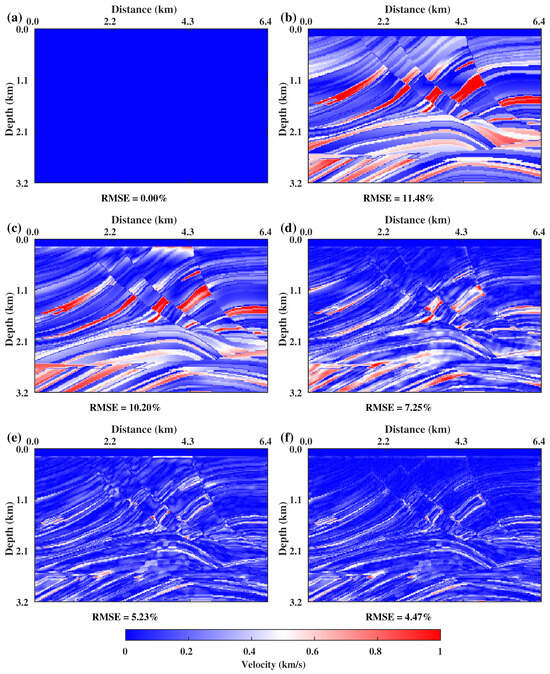
Figure 17.
Residuals of the inversion results with the real model. (a) The true model’s residual. (b) The initial model’s residual. (c) The FTI result’s residual with (b) as the initial model. (d) The FWI result’s residual with (c) as the initial model. (e) The Ms-CNNVI method inversion result’s residual with (c) as the initial model. (f) The FWI result’s residual with (e) as the initial model.
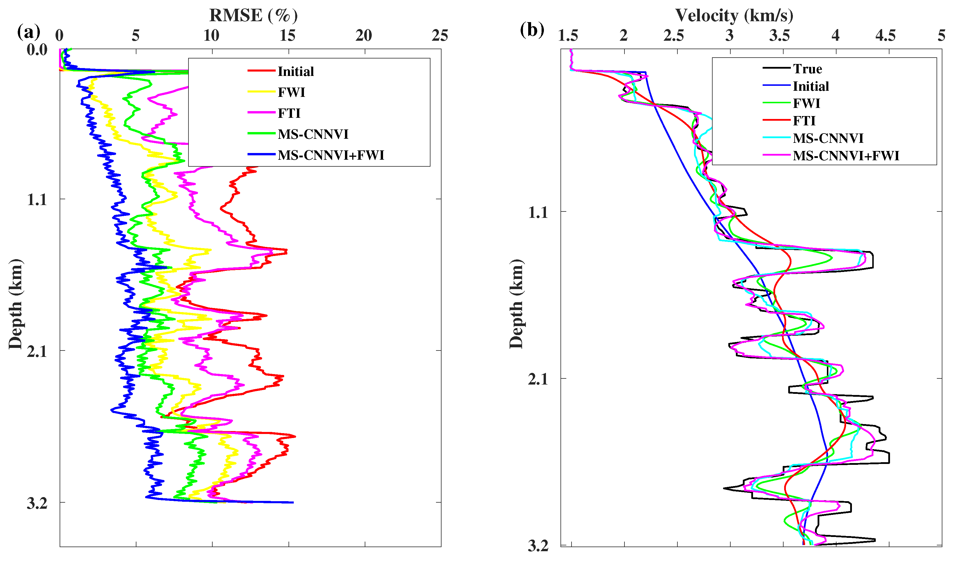
Figure 18a shows the cumulated RMS errors for each position in the same layer. The MS-CNNVI + FWI method exhibited the lowest error across all layers, with our proposed method showcasing significantly more minor errors in the deeper regions compared to the traditional FWI method. These results provide compelling evidence that our proposed strategy for overcoming the limitations of initial models is both feasible and has the potential to achieve further convergence on FWI results. After a comparison of the single trace extracted as illustrated in Figure 18d, it can be inferred that our method, Ms-CNNVI + FWI, achieved the highest velocity accuracy at various positions, thereby showcasing its superiority.
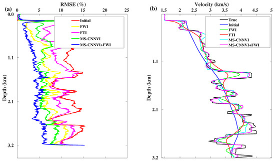
Figure 18.
(a) The cumulated RMS errors for each position in the same layer. (b) Comparison of the single trace velocity extracted from Figure 16.
4. Discussion
Why is a smoothing strategy necessary? First of all, the MS strategy must be combined with a smoothing strategy for implementation. This is because, in the process of inversion from low to high frequencies, each frequency inversion is a CNNVI. At the end of a single-frequency inversion, the output cannot be directly applied to the CNNVI of the next frequency. So, it is necessary to make the inversion processable with a smoothing strategy. Secondly, adding a smoothing strategy can also improve the inversion accuracy of CNNVI, which was partially demonstrated in the ablation experiments in Case 1.
As Figure 15 shows, the method in this paper recovered the boundaries of the salt well. In practice, we could obtain a more accurate velocity model by identifying the boundary of the salt domes and then filling in a fixed velocity value. We could continue the inversion based on this velocity model to obtain a more accurate imaging of the subsalt structure.
Several other directions need to be investigated next in regard to this method. The first is the presented method’s realization of multi-parameter inversion; for example, it can invert parameters such as density and Q-value [38]. It also combines the multi-scale idea with multi-parameter inversion to improve the inversion accuracy of different parameters.
5. Conclusions
In this paper, we propose a multi-scale convolutional neural network (CNN) full-waveform inversion (Ms-CNNVI) method, which incorporates a multi-scale strategy into the CNN-based velocity inversion algorithm. The CNN-based velocity inversion method iteratively estimates the unknown subsurface velocity model using the initial velocity model and its corresponding RTM image. To achieve multi-scale artificial intelligence (AI) inversion, we first integrate a multi-scale strategy from low-frequency inversion to high-frequency inversion into the CNN-based velocity inversion process. This MS strategy greatly enhances the inversion accuracy. Secondly, in the multi-scale AI inversion process, we propose to incorporate a smoothing strategy, which can also improve the inversion accuracy of CNNVI. In addition, we use angle-domain reverse time migration (RTM) for dataset construction in Ms-CNNVI, which significantly improves the efficiency and effectiveness of the inversion. We tested the proposed Ms-CNNVI on several different models and demonstrated its effectiveness in reconstructing the velocity model in different subsurface media. Compared to conventional FWI methods, our approach could better invert the velocity structure of the deep layers. Furthermore, compared to other AI inversion methods, our approach exhibited robust adaptability for different velocity models.
In addition, the method in this paper is restricted by the accuracy of the initial model, which is very similar to FWI. The conventional FWI method is prone to falling into local minima in the absence of a good initial model. The algorithm in this paper also needs the initial model to provide a good background velocity so that the model parcelation algorithm obtains a good training dataset.
Author Contributions
Conceptualization, W.L.; methodology, W.L.; software, W.L. and T.W.; validation, W.L.; formal analysis, W.L.; investigation, W.L.; resources, T.W. and H.L.; data curation, W.L.; writing—original draft preparation, W.L.; writing—review and editing, H.L.; visualization, T.W.; supervision, H.L.; project administration, H.L.; funding acquisition, H.L. All authors have read and agreed to the published version of the manuscript.
Funding
This work was supported by the National Natural Science Foundation of China (Grant No.U20B2014).
Data Availability Statement
Data associated with this research are available and can be obtained by contacting the corresponding author because of funder requirements.
Conflicts of Interest
The authors declare no conflicts of interest.
References
- Symes, W.W. Migration velocity analysis and waveform inversion. Geophys. Prospect. 2008, 56, 765–790. [Google Scholar] [CrossRef]
- Mora, P. Inversion= migration+ tomography. Geophysics 1989, 54, 1575–1586. [Google Scholar] [CrossRef]
- Lailly, P. The Seismic Inverse Problem as a Sequence of Before Stack Migrations; SIAM: Philadelphia, PA, USA, 1983. [Google Scholar]
- Tarantola, A. Inversion of seismic reflection data in the acoustic approximation. Geophysics 1984, 49, 1259–1266. [Google Scholar] [CrossRef]
- Virieux, J.; Operto, S. An overview of full-waveform inversion in exploration geophysics. Geophysics 2009, 74, WCC1–WCC26. [Google Scholar] [CrossRef]
- Li, Z.C.; Qu, Y.M. Research progress on seismic imaging technology. Pet. Sci. 2022, 19, 128–146. [Google Scholar] [CrossRef]
- Hu, L.Z. Wave-field transformations of vertical seismic profiles. Geophysics 1987, 52, 307–321. [Google Scholar] [CrossRef]
- Wang, F.; Chauris, H.; Donno, D.; Calandra, H. Taking advantage of wave field decomposition in full waveform inversion. In Proceedings of the 75th EAGE Conference & Exhibition Incorporating SPE EUROPEC 2013, London, UK, 10–13 June 2013; European Association of Geoscientists & Engineers: Utrecht, The Netherlands, 2013; pp. 1–348. [Google Scholar]
- Lian, S.; Yuan, S.; Wang, G.; Liu, T.; Liu, Y.; Wang, S. Enhancing low-wavenumber components of full-waveform inversion using an improved wavefield decomposition method in the time-space domain. J. Appl. Geophys. 2018, 157, 10–22. [Google Scholar] [CrossRef]
- Wu, Z.; Alkhalifah, T. Efficient scattering-angle enrichment for a nonlinear inversion of the background and perturbations components of a velocity model. Geophys. J. Int. 2017, 210, 1981–1992. [Google Scholar] [CrossRef]
- Yao, G.; Wu, D. Reflection full waveform inversion. Sci. China Earth Sci. 2017, 60, 1783–1794. [Google Scholar] [CrossRef][Green Version]
- Yao, G.; da Silva, N.V.; Warner, M.; Kalinicheva, T. Separation of migration and tomography modes of full-waveform inversion in the plane wave domain. J. Geophys. Res. Solid Earth 2018, 123, 1486–1501. [Google Scholar] [CrossRef]
- Yao, G.; Wu, D.; Wang, S.X. A review on reflection-waveform inversion. Pet. Sci. 2020, 17, 334–351. [Google Scholar] [CrossRef]
- Wang, G.; Guo, Q.; Alkhalifah, T.; Wang, S. Frequency-domain reflection waveform inversion with generalized internal multiple imaging. Geophysics 2021, 86, R701–R710. [Google Scholar] [CrossRef]
- Wu, Y.; Lin, Y.; Zhou, Z. InversionNet: Accurate and efficient seismic waveform inversion with convolutional neural networks. In SEG Technical Program Expanded Abstracts 2018; Society of Exploration Geophysicists: Houston, TX, USA, 2018; pp. 2096–2100. [Google Scholar]
- Yang, F.; Ma, J. Deep-learning inversion: A next-generation seismic velocity model building method. Geophysics 2019, 84, R583–R599. [Google Scholar] [CrossRef]
- Wang, W.; Ma, J. Velocity model building in a crosswell acquisition geometry with image-trained artificial neural networks. Geophysics 2020, 85, U31–U46. [Google Scholar] [CrossRef]
- Liu, B.; Yang, S.; Ren, Y.; Xu, X.; Jiang, P.; Chen, Y. Deep-learning seismic full-waveform inversion for realistic structural models. Geophysics 2021, 86, R31–R44. [Google Scholar] [CrossRef]
- Zhang, W.; Gao, J. Deep-learning full-waveform inversion using seismic migration images. IEEE Trans. Geosci. Remote Sens. 2021, 60, 5901818. [Google Scholar] [CrossRef]
- Zhang, W.; Gao, J.; Gao, Z.; Chen, H. Adjoint-driven deep-learning seismic full-waveform inversion. IEEE Trans. Geosci. Remote Sens. 2020, 59, 8913–8932. [Google Scholar] [CrossRef]
- Wu, Y.; McMechan, G.A.; Wang, Y. CNN-based gradient-free multiparameter reflection full-waveform inversion. In Proceedings of the First International Meeting for Applied Geoscience & Energy, Denver, CO, USA, 26 September–1 October 2021; Society of Exploration Geophysicists: Houston, TX, USA, 2021; pp. 1369–1373. [Google Scholar]
- Wu, Y.; McMechan, G.A.; Wang, Y. Adaptive Feedback Convolutional-Neural-Network-Based High-Resolution Reflection-Waveform Inversion. J. Geophys. Res. Solid Earth 2022, 127, e2022JB024138. [Google Scholar] [CrossRef]
- Muller, A.P.; Bom, C.R.; Costa, J.C.; Klatt, M.; Faria, E.L.; Silva, B.d.S.; de Albuquerque, M.P.; de Albuquerque, M.P. Deep-Tomography: Iterative velocity model building with deep learning. Geophys. J. Int. 2023, 232, 975–989. [Google Scholar] [CrossRef]
- Waheed, U.b.; Alkhalifah, T.; Haghighat, E.; Song, C.; Virieux, J. PINNtomo: Seismic tomography using physics-informed neural networks. arXiv 2021, arXiv:2104.01588. [Google Scholar]
- Song, C.; Alkhalifah, T. Wavefield reconstruction inversion via physics-informed neural networks. IEEE Trans. Geosci. Remote. Sens. 2021, 60, 5908012. [Google Scholar] [CrossRef]
- Bunks, C.; Saleck, F.M.; Zaleski, S.; Chavent, G. Multiscale seismic waveform inversion. Geophysics 1995, 60, 1457–1473. [Google Scholar] [CrossRef]
- Fu, L.; Guo, B.; Schuster, G.T. Multiscale phase inversion of seismic data. Geophysics 2018, 83, R159–R171. [Google Scholar] [CrossRef]
- Choi, Y.; Alkhalifah, T. Source-independent time-domain waveform inversion using convolved wavefields: Application to the encoded multisource waveform inversion. Geophysics 2011, 76, R125–R134. [Google Scholar] [CrossRef]
- Qu, Y.; Li, Z.; Huang, J.; Li, J. Multi-scale full waveform inversion for areas with irregular surface topography in an auxiliary coordinate system. Explor. Geophys. 2018, 49, 68–80. [Google Scholar] [CrossRef]
- Guo, Y.; Huang, J.; Cui, C.; Li, Z.; Fu, L.; Li, Q. Multi-source multi-scale source-independent full waveform inversion. J. Geophys. Eng. 2019, 16, 479–492. [Google Scholar] [CrossRef]
- Liu, D.J.; Huang, J.P.; Wang, Z.Y. Convolution-based multi-scale envelope inversion. Pet. Sci. 2020, 17, 352–362. [Google Scholar] [CrossRef]
- Lu, J.; Wu, C.; Qu, Y.; Zhang, H.; Ma, B. Multi-scale Fusion Network with SR-attention for seismic velocity model building. IEEE Trans. Geosci. Remote Sens. 2023, 61, 5923011. [Google Scholar] [CrossRef]
- Li, W.; Liu, H.; Wu, T.; Huo, S. A High Resolution Velocity Inversion Method Based on Attention Convolutional Neural Network. IEEE Trans. Geosci. Remote Sens. 2023, 61, 5918314. [Google Scholar] [CrossRef]
- Mora, P. Nonlinear two-dimensional elastic inversion of multioffset seismic data. Geophysics 1987, 52, 1211–1228. [Google Scholar] [CrossRef]
- Zhang, Q.; McMechan, G.A. Direct vector-field method to obtain angle-domain common-image gathers from isotropic acoustic and elastic reverse time migration. Geophysics 2011, 76, WB135–WB149. [Google Scholar] [CrossRef]
- Li, W.; Wu, T.; Liu, H. Structure-Preserving Random Noise Attenuation Method for Seismic Data Based on a Flexible Attention CNN. Remote Sens. 2022, 14, 5240. [Google Scholar] [CrossRef]
- Liu, L.; Wu, Y.; Guo, B.; Han, S.; Luo, Y. Near-surface velocity estimation using source-domain full traveltime inversion and early-arrival waveform inversion. Geophysics 2018, 83, R335–R344. [Google Scholar] [CrossRef]
- Wang, Y.; Qu, Y. Q-compensated full waveform inversion for velocity and density. Explor. Geophys. 2022, 53, 487–500. [Google Scholar] [CrossRef]
Disclaimer/Publisher’s Note: The statements, opinions and data contained in all publications are solely those of the individual author(s) and contributor(s) and not of MDPI and/or the editor(s). MDPI and/or the editor(s) disclaim responsibility for any injury to people or property resulting from any ideas, methods, instructions or products referred to in the content. |
© 2024 by the authors. Licensee MDPI, Basel, Switzerland. This article is an open access article distributed under the terms and conditions of the Creative Commons Attribution (CC BY) license (https://creativecommons.org/licenses/by/4.0/).

