
High Spatial Resolution Leaf Area Index Estimation for Woodland in Saihanba Forestry Center, China


Abstract
1. Introduction
2. Data
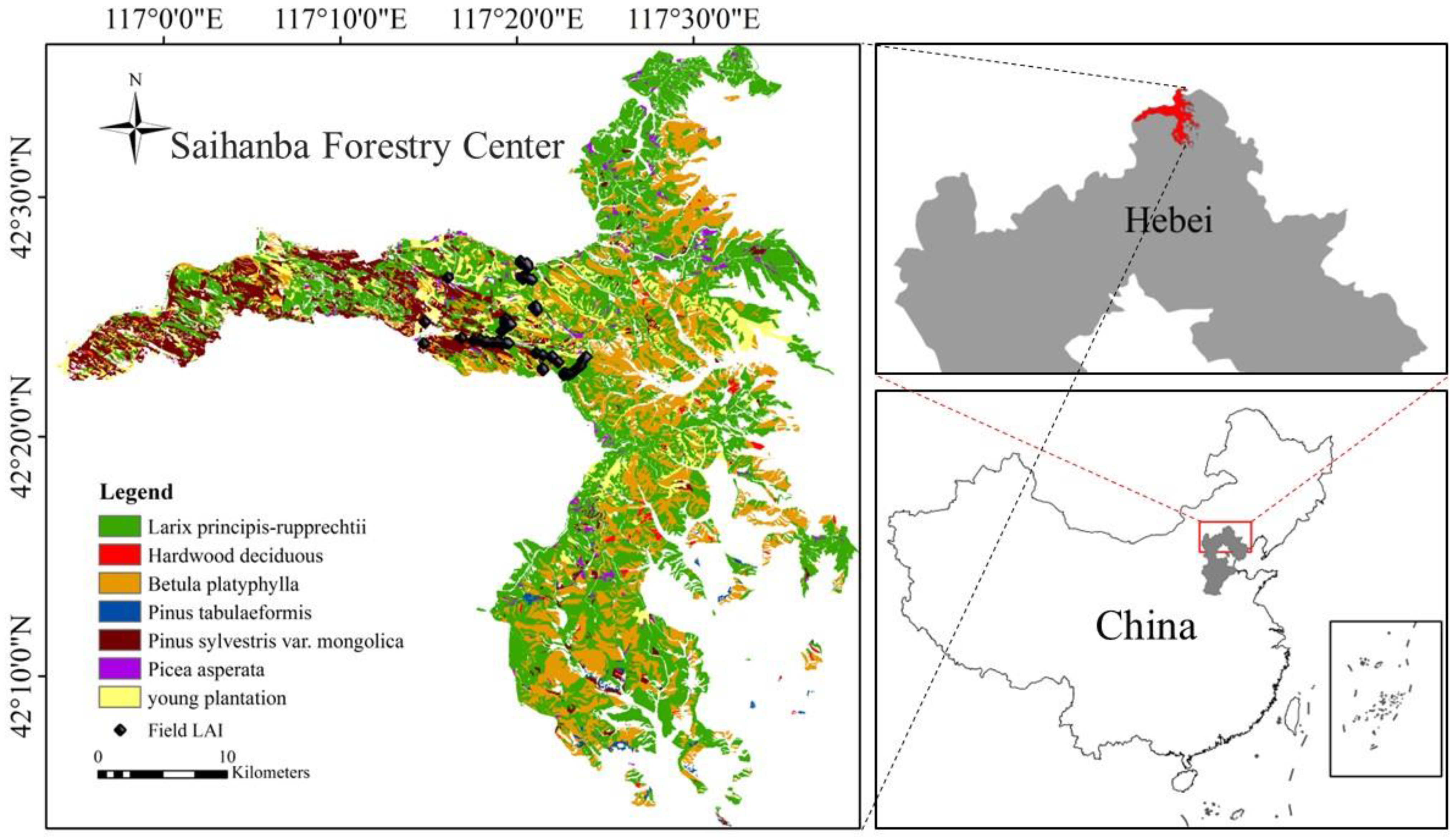
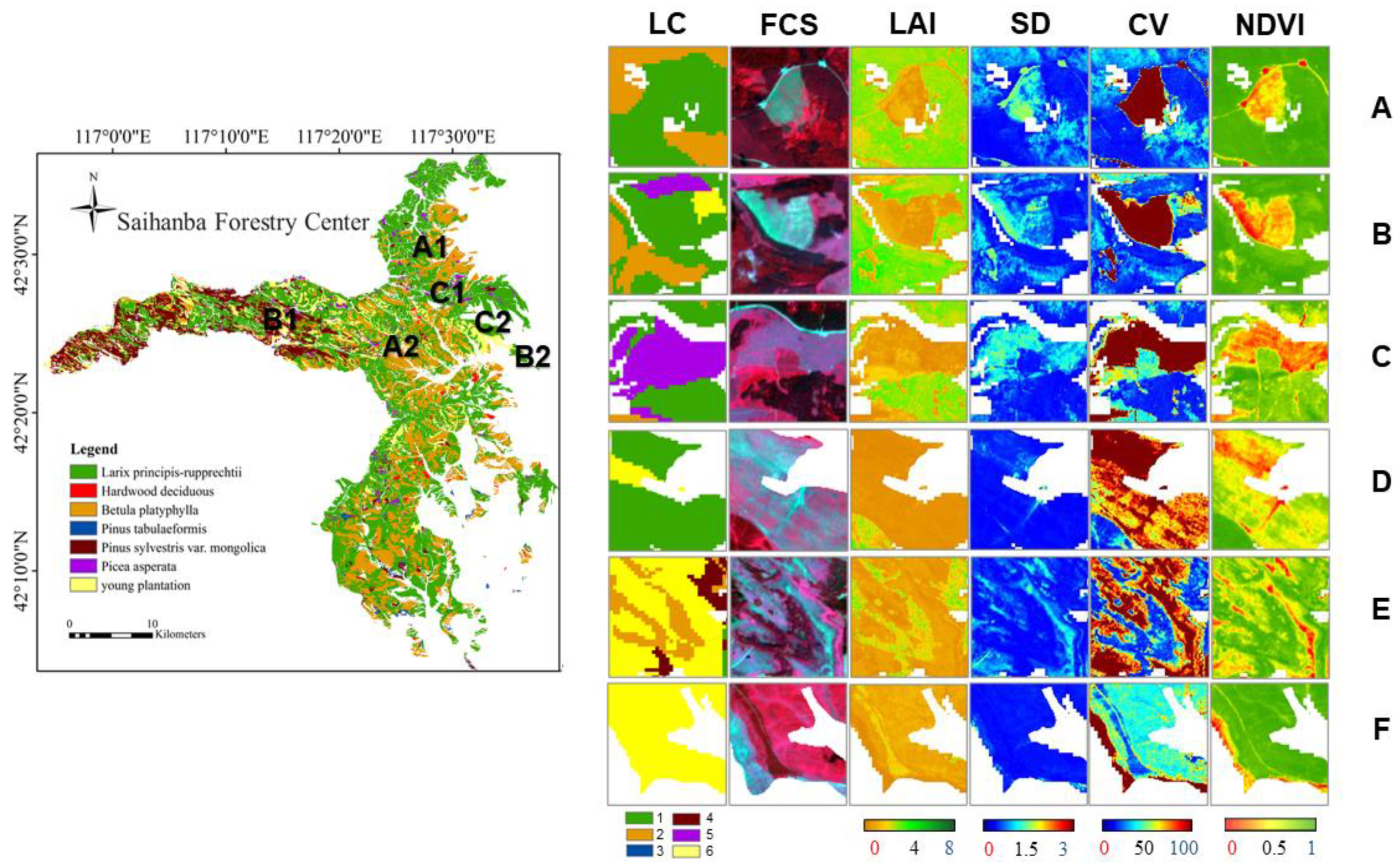
2.1. Study Area
2.2. Field Data
2.3. Sentinel-2 Data
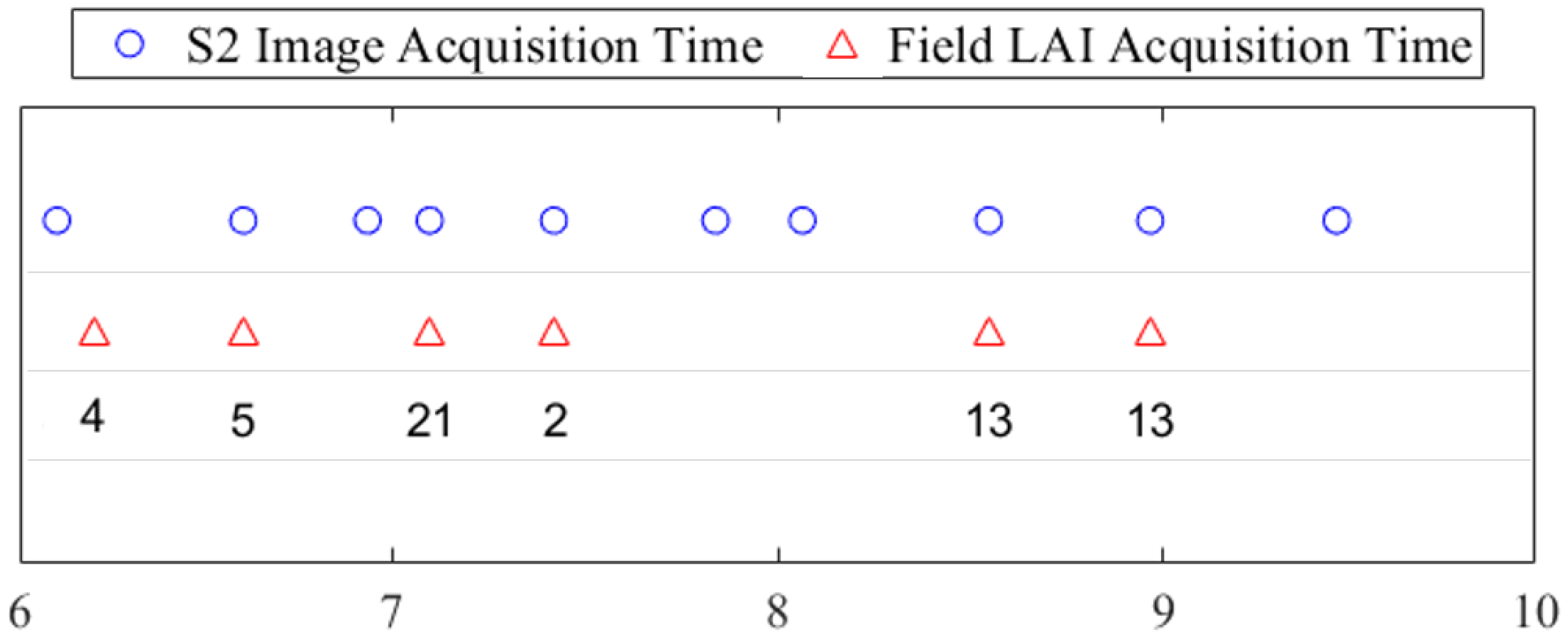
2.4. Matching Sentinel-2 Reflectance and Field LAI
3. Methods
3.1. Principle of Involved Models
3.1.1. Gaussian Process Regression
3.1.2. Backpack Neural Network Based on Simulated Annealing Algorithm
3.2. Method Implementation and Verification
4. Result
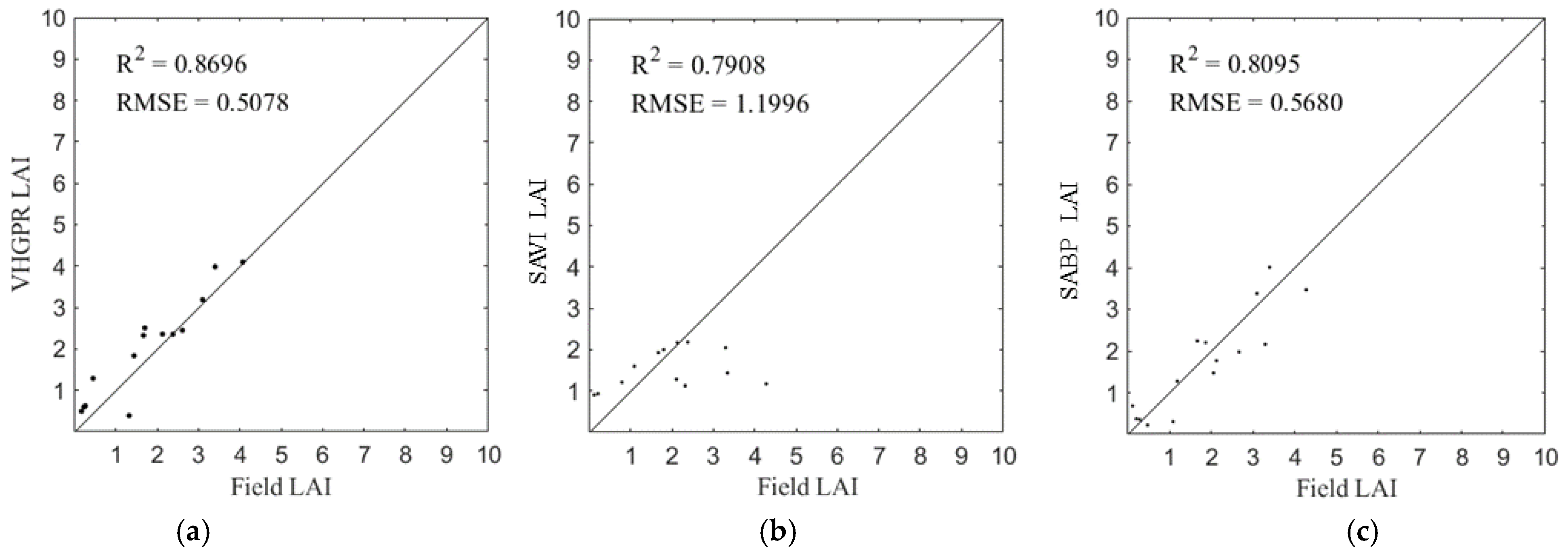
4.1. Validation with Field Data
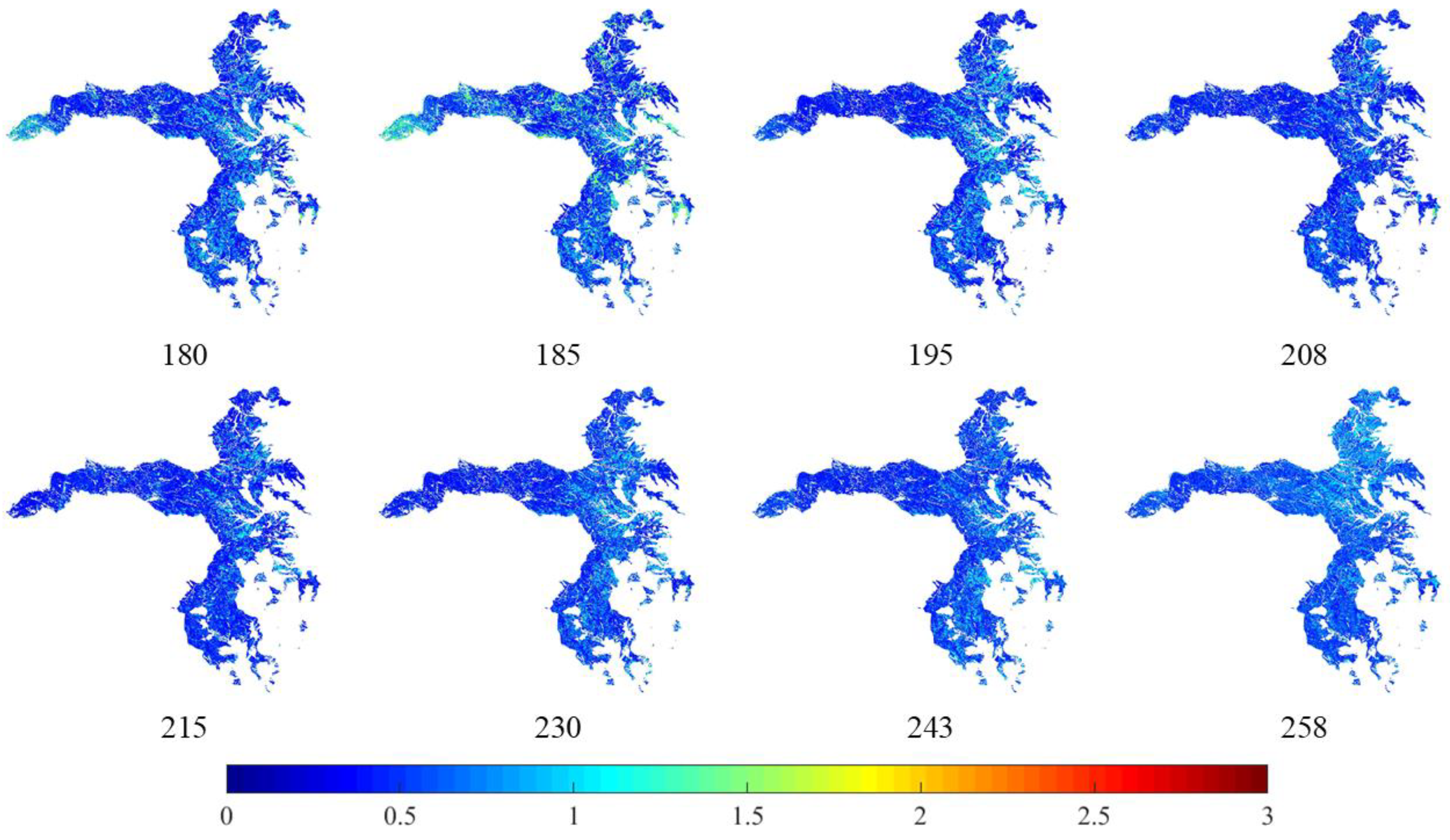
4.2. SFC LAI Distribution Map Generated by VHGPR
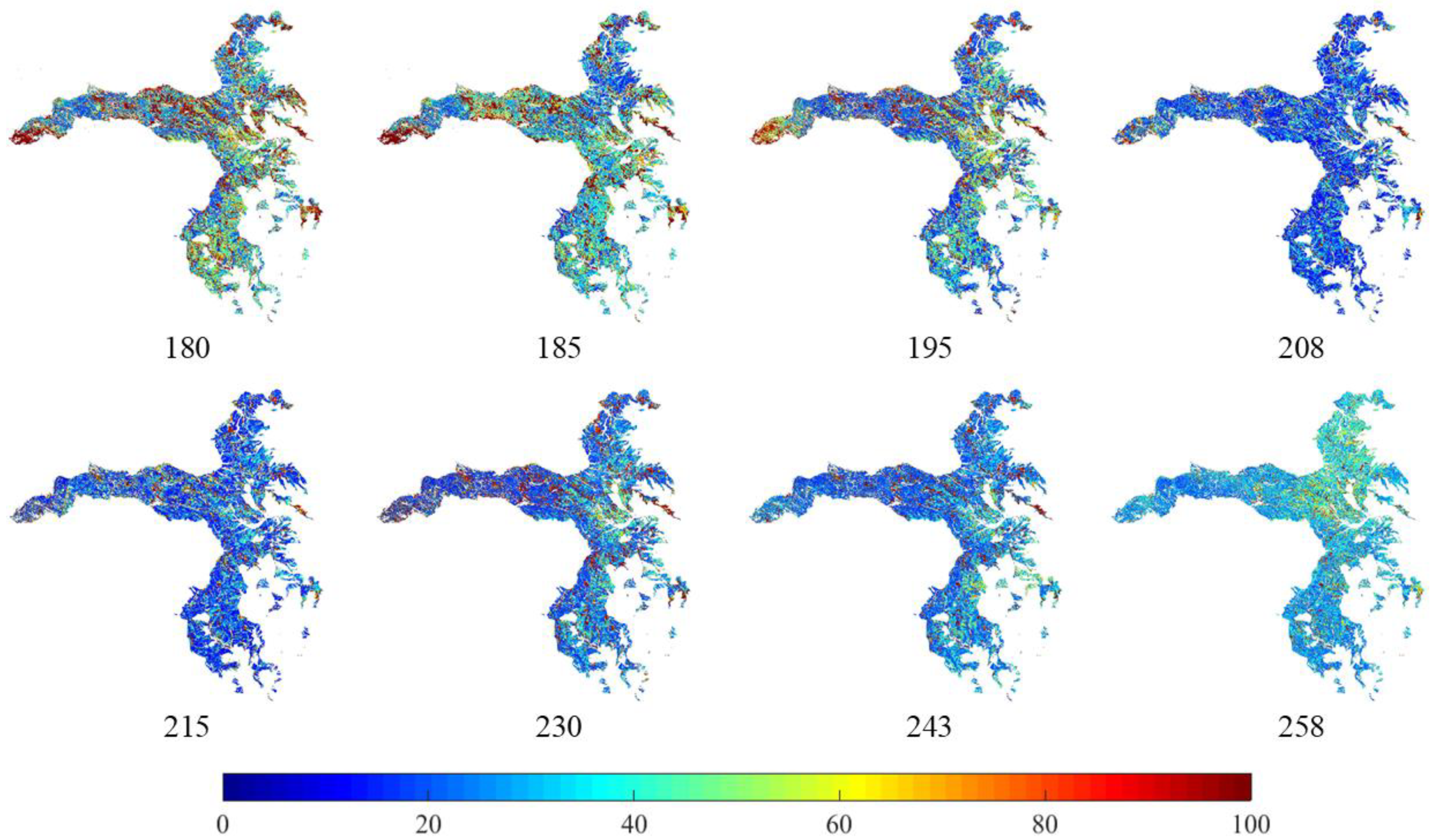
4.3. Uncertainties and Relative Uncertainties of SFC LAI Distribution Map
5. Discussion
5.1. Errors from Field LAI Data
5.2. Advantage of VHGPR Methods
5.3. Further Work for LAI Estimated by VHGPR
5.4. Evaluation of LAI Time Series Distribution Maps
6. Conclusions
Author Contributions
Funding
Data Availability Statement
Conflicts of Interest
References
- Chen, J.M.; Black, T. Defining leaf area index for non-flat leaves. Plant Cell Environ. 1992, 15, 421–429. [Google Scholar] [CrossRef]
- Yang, W.; Tan, B.; Huang, D.; Rautiainen, M.; Shabanov, N.V.; Wang, Y.; Privette, J.L.; Huemmrich, K.F.; Fensholt, R.; Sandholt, I.; et al. MODIS leaf area index products: From validation to algorithm improvement. IEEE Trans. Geosci. Remote Sens. 2006, 44, 1885–1898. [Google Scholar] [CrossRef]
- Baret, F.; Weiss, M.; Lacaze, R.; Camacho, F.; Makhmara, H.; Pacholcyzk, P.; Smets, B. GEOV1: LAI and FAPAR essential climate variables and FCOVER global time series capitalizing over existing products. Part1: Principles of development and production. Remote Sens. Environ. 2013, 137, 299–309. [Google Scholar] [CrossRef]
- Fang, H.; Baret, F.; Plummer, S.; Schaepman-Strub, G. An overview of global leaf area index (LAI): Methods, products, validation, and applications. Rev. Geophys. 2019, 57, 739–799. [Google Scholar] [CrossRef]
- Liang, S.; Yi, Q.; Liu, J. Vegetation dynamics and responses to recent climate change in Xinjiang using leaf area index as an indicator. Ecol. Indic. 2015, 58, 64–76. [Google Scholar]
- Chen, Y.; Zhang, Z.; Tao, F. Improving regional winter wheat yield estimation through assimilation of phenology and leaf area index from remote sensing data. Eur. J. Agron. 2018, 101, 163–173. [Google Scholar] [CrossRef]
- Tripathi, A.M.; Pohanková, E.; Fischer, M.; Orság, M.; Trnka, M.; Klem, K.; Marek, M.V. The evaluation of radiation use efficiency and leaf area index development for the estimation of biomass accumulation in short rotation poplar and annual field crops. Forests 2018, 9, 168. [Google Scholar] [CrossRef]
- Deng, F.; Chen, J.M.; Plummer, S.; Chen, M.; Pisek, J. Algorithm for global leaf area index retrieval using satellite imagery. IEEE Trans. Geosci. Remote Sens. 2006, 44, 2219–2229. [Google Scholar] [CrossRef]
- Verrelst, J.; Rivera, J.P.; Veroustraete, F.; Muñoz-Marí, J.; Clevers, J.G.; Camps-Valls, G.; Moreno, J. Experimental Sentinel-2 LAI estimation using parametric, non-parametric and physical retrieval methods—A comparison. ISPRS J. Photogramm. Remote Sens. 2015, 108, 260–272. [Google Scholar] [CrossRef]
- Chaurasia, S.; Nigam, R.; Bhattacharya, B.; Sridhar, V.; Mallick, K.; Vyas, S.; Patel, N.; Mukherjee, J.; Shekhar, C.; Kumar, D. Development of regional wheat VI-LAI models using Resourcesat-1 AWiFS data. J. Earth Syst. Sci. 2011, 120, 1113–1125. [Google Scholar] [CrossRef]
- Goswami, S.; Gamon, J.; Vargas, S.; Tweedie, C. Relationships of NDVI, Biomass, and Leaf Area Index (LAI) for Six Key Plant Species in Barrow, Alaska; 2167-9843; PeerJ PrePrints: London, UK, 2015. [Google Scholar]
- Walthall, C.; Dulaney, W.; Anderson, M.; Norman, J.; Fang, H.; Liang, S. A comparison of empirical and neural network approaches for estimating corn and soybean leaf area index from Landsat ETM+ imagery. Remote Sens. Environ. 2004, 92, 465–474. [Google Scholar] [CrossRef]
- Cañete-Salinas, P.; Zamudio, F.; Yáñez, M.; Gajardo, J.; Valdés, H.; Espinosa, C.; Venegas, J.; Retamal, L.; Ortega-Farias, S.; Acevedo-Opazo, C. Evaluation of models to determine LAI on poplar stands using spectral indices from Sentinel-2 satellite images. Ecol. Model. 2020, 428, 109058. [Google Scholar] [CrossRef]
- Qiao, K.; Zhu, W.; Xie, Z.; Li, P. Estimating the seasonal dynamics of the leaf area index using piecewise LAI-VI relationships based on phenophases. Remote Sens. 2019, 11, 689. [Google Scholar] [CrossRef]
- Ariza-Carricondo, C.; Di Mauro, F.; de Beeck, M.O.; Roland, M.; Gielen, B.; Vitale, D.; Ceulemans, R.; Papale, D. A comparison of different methods for assessing leaf area index in four canopy types. Cent. Eur. For. J. 2019, 65, 67–80. [Google Scholar] [CrossRef]
- Houborg, R.; McCabe, M.F. A hybrid training approach for leaf area index estimation via Cubist and random forests machine-learning. ISPRS J. Photogramm. Remote Sens. 2018, 135, 173–188. [Google Scholar] [CrossRef]
- Xie, Q.; Dash, J.; Huang, W.; Peng, D.; Qin, Q.; Mortimer, H.; Casa, R.; Pignatti, S.; Laneve, G.; Pascucci, S. Vegetation indices combining the red and red-edge spectral information for leaf area index retrieval. IEEE J. Sel. Top. Appl. Earth Obs. Remote Sens. 2018, 11, 1482–1493. [Google Scholar] [CrossRef]
- Song, Y.; Wang, J.; Shang, J. Estimating effective leaf area index of winter wheat using simulated observation on unmanned aerial vehicle-based point cloud data. IEEE J. Sel. Top. Appl. Earth Obs. Remote Sens. 2020, 13, 2874–2887. [Google Scholar] [CrossRef]
- Danner, M.; Berger, K.; Wocher, M.; Mauser, W.; Hank, T. Efficient RTM-based training of machine learning regression algorithms to quantify biophysical & biochemical traits of agricultural crops. ISPRS J. Photogramm. Remote Sens. 2021, 173, 278–296. [Google Scholar]
- Ali, A.M.; Darvishzadeh, R.; Skidmore, A.K. Retrieval of specific leaf area from landsat-8 surface reflectance data using statistical and physical models. IEEE J. Sel. Top. Appl. Earth Obs. Remote Sens. 2017, 10, 3529–3536. [Google Scholar] [CrossRef]
- Darvishzadeh, R.; Atzberger, C.; Skidmore, A.; Schlerf, M. Mapping grassland leaf area index with airborne hyperspectral imagery: A comparison study of statistical approaches and inversion of radiative transfer models. ISPRS J. Photogramm. Remote Sens. 2011, 66, 894–906. [Google Scholar] [CrossRef]
- Shiklomanov, A.N.; Dietze, M.C.; Viskari, T.; Townsend, P.A.; Serbin, S.P. Quantifying the influences of spectral resolution on uncertainty in leaf trait estimates through a Bayesian approach to RTM inversion. Remote Sens. Environ. 2016, 183, 226–238. [Google Scholar] [CrossRef]
- Wang, X.; Jia, K.; Liang, S.; Zhang, Y. Fractional vegetation cover estimation method through dynamic Bayesian network combining radiative transfer model and crop growth model. IEEE Trans. Geosci. Remote Sens. 2016, 54, 7442–7450. [Google Scholar] [CrossRef]
- Servera, J.V.; Alonso, L.; Martino, L.; Sabater, N.; Verrelst, J.; Camps-Valls, G.; Moreno, J. Gradient-based automatic lookup table generator for radiative transfer models. IEEE Trans. Geosci. Remote Sens. 2018, 57, 1040–1048. [Google Scholar] [CrossRef]
- Xu, X.; Lu, J.; Zhang, N.; Yang, T.; He, J.; Yao, X.; Cheng, T.; Zhu, Y.; Cao, W.; Tian, Y. Inversion of rice canopy chlorophyll content and leaf area index based on coupling of radiative transfer and Bayesian network models. ISPRS J. Photogramm. Remote Sens. 2019, 150, 185–196. [Google Scholar] [CrossRef]
- Verrelst, J.; Rivera, J.P.; Leonenko, G.; Alonso, L.; Moreno, J. Optimizing LUT-Based RTM Inversion for Semiautomatic Mapping of Crop Biophysical Parameters from Sentinel-2 and -3 Data: Role of Cost Functions. IEEE Trans. Geosci. Remote Sens. 2014, 52, 257–269. [Google Scholar] [CrossRef]
- Pan, H.; Chen, Z.; Ren, J.; Li, H.; Wu, S. Modeling winter wheat leaf area index and canopy water content with three different approaches using Sentinel-2 multispectral instrument data. IEEE J. Sel. Top. Appl. Earth Obs. Remote Sens. 2018, 12, 482–492. [Google Scholar] [CrossRef]
- Myneni, R.; Park, Y. MODIS Collection 6 (C6) LAI/FPAR Product User’s Guide. 2015. Available online: https://lpdaac.usgs.gov/documents/624/-MOD15_User_Guide_V6.pdf (accessed on 15 February 2024).
- Wang, L.; Wang, P.; Liang, S.; Qi, X.; Li, L.; Xu, L. Monitoring maize growth conditions by training a BP neural network with remotely sensed vegetation temperature condition index and leaf area index. Comput. Electron. Agric. 2019, 160, 82–90. [Google Scholar] [CrossRef]
- Wang, L.; Chang, Q.; Yang, J.; Zhang, X.; Li, F. Estimation of paddy rice leaf area index using machine learning methods based on hyperspectral data from multi-year experiments. PLoS ONE 2018, 13, e0207624. [Google Scholar] [CrossRef]
- Verger, A.; Baret, F.; Weiss, M. Performances of neural networks for deriving LAI estimates from existing CYCLOPES and MODIS products. Remote Sens. Environ. 2008, 112, 2789–2803. [Google Scholar] [CrossRef]
- Xue, H.; Wang, C.; Zhou, H.; Wang, J.; Wan, H. BP Neural Network Based on Simulated Annealing Algorithm for High Resolution LAI Retrieval. Remote Sens. Technol. Appl. 2020, 35, 1057–1069. [Google Scholar]
- Srinet, R.; Nandy, S.; Patel, N.R. Estimating leaf area index and light extinction coefficient using Random Forest regression algorithm in a tropical moist deciduous forest, India. Ecol. Inform. 2019, 52, 94–102. [Google Scholar] [CrossRef]
- Sinha, S.K.; Padalia, H.; Dasgupta, A.; Verrelst, J.; Rivera, J.P. Estimation of leaf area index using PROSAIL based LUT inversion, MLRA-GPR and empirical models: Case study of tropical deciduous forest plantation, North India. Int. J. Appl. Earth Obs. Geoinf. 2020, 86, 102027. [Google Scholar] [CrossRef]
- Zhang, Y.; Yang, J.; Liu, X.; Du, L.; Shi, S.; Sun, J.; Chen, B. Estimation of multi-species leaf area index based on Chinese GF-1 satellite data using look-up table and gaussian process regression methods. Sensors 2020, 20, 2460. [Google Scholar] [CrossRef]
- Verrelst, J.; Camps-Valls, G.; Muñoz-Marí, J.; Rivera, J.P.; Veroustraete, F.; Clevers, J.G.; Moreno, J. Optical remote sensing and the retrieval of terrestrial vegetation bio-geophysical properties—A review. ISPRS J. Photogramm. Remote Sens. 2015, 108, 273–290. [Google Scholar] [CrossRef]
- Estévez, J.; Vicent, J.; Rivera-Caicedo, J.P.; Morcillo-Pallarés, P.; Vuolo, F.; Sabater, N.; Camps-Valls, G.; Moreno, J.; Verrelst, J. Gaussian processes retrieval of LAI from Sentinel-2 top-of-atmosphere radiance data. ISPRS J. Photogramm. Remote Sens. 2020, 167, 289–304. [Google Scholar] [CrossRef] [PubMed]
- Lázaro-Gredilla, M.; Titsias, M.K.; Verrelst, J.; Camps-Valls, G. Retrieval of biophysical parameters with heteroscedastic Gaussian processes. IEEE Geosci. Remote Sens. Lett. 2013, 11, 838–842. [Google Scholar] [CrossRef]
- Lázaro-Gredilla, M.; Titsias, M.K. Variational heteroscedastic Gaussian process regression. In Proceedings of the ICML, Bellevue, WA, USA, 28 June–2 July 2011. [Google Scholar]
- Muñoz-Marí, J.; Verrelst, J.; Lázaro-Gredilla, M.; Camps-Vails, G. Biophysical parameter retrieval with warped Gaussian processes. In Proceedings of the 2015 IEEE International Geoscience and Remote Sensing Symposium (IGARSS), Milan, Italy, 26–31 July 2015; pp. 13–16. [Google Scholar]
- Verrelst, J.; Berger, K.; Rivera-Caicedo, J.P. Intelligent sampling for vegetation nitrogen mapping based on hybrid machine learning algorithms. IEEE Geosci. Remote Sens. Lett. 2020, 18, 2038–2042. [Google Scholar] [CrossRef]
- Tian, J.; Zhu, X.; Shen, Z.; Wu, J.; Xu, S.; Liang, Z.; Wang, J. Investigating the urban-induced microclimate effects on winter wheat spring phenology using Sentinel-2 time series. Agric. For. Meteorol. 2020, 294, 108153. [Google Scholar] [CrossRef]
- Li, L.; Zhou, X.; Chen, L.; Chen, L.; Zhang, Y.; Liu, Y. Estimating urban vegetation biomass from Sentinel-2A image data. Forests 2020, 11, 125. [Google Scholar] [CrossRef]
- Zhang, X.; Song, P. Estimating urban evapotranspiration at 10 m resolution using vegetation information from Sentinel-2: A case study for the Beijing Sponge City. Remote Sens. 2021, 13, 2048. [Google Scholar] [CrossRef]
- Gao, T.; Zhu, J.; Zheng, X.; Shang, G.; Huang, L.; Wu, S. Mapping spatial distribution of larch plantations from multi-seasonal Landsat-8 OLI imagery and multi-scale textures using random forests. Remote Sens. 2015, 7, 1702–1720. [Google Scholar] [CrossRef]
- Yan, G.; Zhao, T.; Mu, X.; Wen, J.; Pang, Y.; Jia, L.; Zhang, Y.; Chen, D.; Yao, C.; Cao, Z.; et al. Comprehensive remote sensing experiment of carbon cycle, water cycle and energy balance in Luan River Basin. Natl. Remote Sens. Bull. 2021, 25, 856–870. [Google Scholar] [CrossRef]
- Mu, X.; Yan, G.J.; Zhou, H.M.; Pang, Y.; Qiu, F.; Zhang, Q.; Zhang, Y.G.; Xie, D.H.; Zhou, Y.J.; Zhao, T.J.; et al. Airborne comprehensive remote sensing experiment of forest and grass resources in Xiaoluan River Basin. Natl. Remote Sens. Bull. 2021, 25, 888–903. [Google Scholar] [CrossRef]
- Zhou, H.; Zhang, G.; Wang, C.; Wang, J.; Cheng, S.; Xue, H.; Wan, H.; Zhang, L. Time series high-resolution leaf area index estimation and change monitoring in the Saihanba area. Natl. Remote Sens. Bull. 2021, 25, 1000–1012. [Google Scholar] [CrossRef]
- Bakó, G.; Fülöp, G.; Szabó, B. Detection of Invasive Woody Increment with the Analysis of Landsat Images. In Proceedings of the Forum of Young Geoinformaticians 2014, Technical University, Zvolen, Slovakia, 5–6 June 2014; pp. 63–71. [Google Scholar]
- Schulz, E.; Speekenbrink, M.; Krause, A. A tutorial on Gaussian process regression: Modelling, exploring, and exploiting functions. J. Math. Psychol. 2018, 85, 1–16. [Google Scholar] [CrossRef]
- Savitsky, T.; Vannucci, M.; Sha, N. Variable selection for nonparametric Gaussian process priors: Models and computational strategies. Stat. Sci. Rev. J. Inst. Math. Stat. 2011, 26, 130. [Google Scholar] [CrossRef]
- Bazi, Y.; Melgani, F. Gaussian process approach to remote sensing image classification. IEEE Trans. Geosci. Remote Sens. 2009, 48, 186–197. [Google Scholar] [CrossRef]
- Camps-Valls, G.; Verrelst, J.; Munoz-Mari, J.; Laparra, V.; Mateo-Jimenez, F.; Gomez-Dans, J. A survey on Gaussian processes for earth-observation data analysis: A comprehensive investigation. IEEE Geosci. Remote Sens. Mag. 2016, 4, 58–78. [Google Scholar] [CrossRef]
- Liu, X.; Zhu, X.; Zhang, Q.; Yang, T.; Pan, Y.; Sun, P. A remote sensing and artificial neural network-based integrated agricultural drought index: Index development and applications. Catena 2020, 186, 104394. [Google Scholar] [CrossRef]
- Zheng, G.; Moskal, L.M. Retrieving leaf area index (LAI) using remote sensing: Theories, methods and sensors. Sensors 2009, 9, 2719–2745. [Google Scholar] [CrossRef]
- Yuan, Q.; Shen, H.; Li, T.; Li, Z.; Li, S.; Jiang, Y.; Xu, H.; Tan, W.; Yang, Q.; Wang, J.; et al. Deep learning in environmental remote sensing: Achievements and challenges. Remote Sens. Environ. 2020, 241, 111716. [Google Scholar] [CrossRef]
- Chen, L.; Zhao, J.; Wang, W.; Xu, Q. A gaussian approximation of marginal likelihood in relevance vector machine for industrial data with input noise. IEEE Trans. Instrum. Meas. 2020, 70, 1–12. [Google Scholar] [CrossRef]
- Dehghan-Shoar, M.H.; Orsi, A.A.; Pullanagari, R.R.; Yule, I.J. A hybrid model to predict nitrogen concentration in heterogeneous grassland using field spectroscopy. Remote Sens. Environ. 2023, 285, 113385. [Google Scholar] [CrossRef]
- Shi, H.; Xiao, Z.; Tian, X. Exploration of machine learning techniques in emulating a coupled soil–canopy–atmosphere radiative transfer model for multi-parameter estimation from satellite observations. IEEE Trans. Geosci. Remote Sens. 2019, 57, 8522–8533. [Google Scholar] [CrossRef]
- Jin, H.; Li, A.; Bian, J.; Nan, X.; Zhao, W.; Zhang, Z.; Yin, G. Intercomparison and validation of MODIS and GLASS leaf area index (LAI) products over mountain areas: A case study in southwestern China. Int. J. Appl. Earth Obs. Geoinf. 2017, 55, 52–67. [Google Scholar] [CrossRef]
- Yu, W.; Li, J.; Liu, Q.; Yin, G.; Zeng, Y.; Lin, S.; Zhao, J. A simulation-based analysis of topographic effects on LAI inversion over sloped terrain. IEEE J. Sel. Top. Appl. Earth Obs. Remote Sens. 2020, 13, 794–806. [Google Scholar] [CrossRef]
- Jin, H.; Li, A.; Xu, W.; Xiao, Z.; Jiang, J.; Xue, H. Evaluation of topographic effects on multiscale leaf area index estimation using remotely sensed observations from multiple sensors. ISPRS J. Photogramm. Remote Sens. 2019, 154, 176–188. [Google Scholar] [CrossRef]
- Gao, F.; Masek, J.; Schwaller, M.; Hall, F. On the blending of the Landsat and MODIS surface reflectance: Predicting daily Landsat surface reflectance. IEEE Trans. Geosci. Remote Sens. 2006, 44, 2207–2218. [Google Scholar]
- Huang, H.; Huang, J.; Wu, Y.; Zhuo, W.; Song, J.; Li, X.; Li, L.; Su, W.; Ma, H.; Liang, S. The improved winter wheat yield estimation by assimilating GLASS LAI into a crop growth model with the proposed Bayesian posterior-based ensemble Kalman filter. IEEE Trans. Geosci. Remote Sens. 2023, 61, 1–18. [Google Scholar] [CrossRef]
- Ling, X.; Fu, C.; Yang, Z.; Guo, W. Comparison of different sequential assimilation algorithms for satellite-derived leaf area index using the Data Assimilation Research Testbed (version Lanai). Geosci. Model Dev. 2019, 12, 3119–3133. [Google Scholar] [CrossRef]
- Zhang, K.; Zhou, H.; Wang, J.; Xue, H. Estimation and validation of high temporal and spatial resolution albedo. In Proceedings of the 2013 IEEE International Geoscience and Remote Sensing Symposium-IGARSS, Melbourne, Australia, 21–26 July 2013; pp. 2888–2891. [Google Scholar]
- Liu, W.; Feng, Q.; Zhang, F. Spatial-temporal variation characteristics of NPP in the Heihe River Basin, northwestern China, in a recent 10-year period calculated by casa model. J. Coast. Res. 2017, 80, 36–47. [Google Scholar] [CrossRef]
- Xiao, Z.; Liang, S.; Wang, J.; Yang, X.; Song, J. Long-Time-Series Global Land Surface Satellite Leaf Area Index Product Derived from MODIS and AVHRR Surface Reflectance. IEEE Trans. Geosci. Remote Sens. 2016, 54, 5301–5318. [Google Scholar] [CrossRef]
- Liu, Y.; Xiao, J.; Ju, W.; Zhu, G.; Wu, X.; Fan, W.; Li, D.; Zhou, Y. Satellite-derived LAI products exhibit large discrepancies and can lead to substantial uncertainty in simulated carbon and water fluxes. Remote Sens. Environ. 2018, 206, 174–188. [Google Scholar] [CrossRef]
- Guay, K.C.; Beck, P.S.; Berner, L.T.; Goetz, S.J.; Baccini, A.; Buermann, W. Vegetation productivity patterns at high northern latitudes: A multi-sensor satellite data assessment. Glob. Change Biol. 2014, 20, 3147–3158. [Google Scholar] [CrossRef]
- Li, Z.; Huang, C.; Zhu, Z.; Gao, F.; Tang, H.; Xin, X.; Ding, L.; Shen, B.; Liu, J.; Chen, B. Mapping daily leaf area index at 30 m resolution over a meadow steppe area by fusing Landsat, Sentinel-2A and MODIS data. Int. J. Remote Sens. 2018, 39, 9025–9053. [Google Scholar] [CrossRef]
- Zhang, J. Multi-source remote sensing data fusion: Status and trends. Int. J. Image Data Fusion 2010, 1, 5–24. [Google Scholar] [CrossRef]


| Band | Description | Wavelength (µm) | Resolution (m) |
|---|---|---|---|
| 1 | Coastal aerosol | 0.433–0.453 | 60 |
| 2 | Blue * | 0.458–0.523 | 10 |
| 3 | Green * | 0.543–0.578 | 10 |
| 4 | Red * | 0.650–0.680 | 10 |
| 5 | Vegetation red edge | 0.698–0.713 | 20 |
| 6 | Vegetation red edge | 0.733–0.748 | 20 |
| 7 | Vegetation red edge | 0.773–0.793 | 20 |
| 8 | NIR * | 0.785–0.900 | 10 |
| 8A | Narrow NIR | 0.855–0.875 | 20 |
| 9 | Water vapor | 0.935–0.955 | 60 |
| 10 | SWIR–cirrus | 1.365–1.385 | 60 |
| 11 | SWIR-1 | 1.565–1.655 | 20 |
| 12 | SWIR-2 | 2.100–2.280 | 20 |
| DOY | Mean SD | Mean CV (%) |
|---|---|---|
| 180 | 0.1212 | 10.2851 |
| 185 | 0.1360 | 10.0728 |
| 195 | 0.1176 | 7.5763 |
| 208 | 0.1104 | 5.0239 |
| 215 | 0.1059 | 5.2505 |
| 230 | 0.1170 | 6.7886 |
| 243 | 0.1167 | 6.6019 |
| 258 | 0.1269 | 8.5541 |
Disclaimer/Publisher’s Note: The statements, opinions and data contained in all publications are solely those of the individual author(s) and contributor(s) and not of MDPI and/or the editor(s). MDPI and/or the editor(s) disclaim responsibility for any injury to people or property resulting from any ideas, methods, instructions or products referred to in the content. |
© 2024 by the authors. Licensee MDPI, Basel, Switzerland. This article is an open access article distributed under the terms and conditions of the Creative Commons Attribution (CC BY) license (https://creativecommons.org/licenses/by/4.0/).
Share and Cite
Wang, C.; Zhou, H.; Zhang, G.; Duan, J.; Lin, M. High Spatial Resolution Leaf Area Index Estimation for Woodland in Saihanba Forestry Center, China. Remote Sens. 2024, 16, 764. https://doi.org/10.3390/rs16050764
Wang C, Zhou H, Zhang G, Duan J, Lin M. High Spatial Resolution Leaf Area Index Estimation for Woodland in Saihanba Forestry Center, China. Remote Sensing. 2024; 16(5):764. https://doi.org/10.3390/rs16050764
Chicago/Turabian StyleWang, Changjing, Hongmin Zhou, Guodong Zhang, Jianguo Duan, and Moxiao Lin. 2024. "High Spatial Resolution Leaf Area Index Estimation for Woodland in Saihanba Forestry Center, China" Remote Sensing 16, no. 5: 764. https://doi.org/10.3390/rs16050764
APA StyleWang, C., Zhou, H., Zhang, G., Duan, J., & Lin, M. (2024). High Spatial Resolution Leaf Area Index Estimation for Woodland in Saihanba Forestry Center, China. Remote Sensing, 16(5), 764. https://doi.org/10.3390/rs16050764