Article

Extraction and Analysis of Grasshopper Potential Habitat in Hulunbuir Based on the Maximum Entropy Model

1
State Key Laboratory of Digital Earth Science, Aerospace Information Research Institute, Chinese Academy of Sciences, Beijing 100094, China
2
University of Chinese Academy of Sciences, Beijing 100049, China
3
Key Laboratory of Biohazard Monitoring and Green Prevention and Control in Artificial Grassland, Ministry of Agriculture and Rural Affairs, Hohhot 010010, China
*
Author to whom correspondence should be addressed.
Remote Sens. 2024, 16(5), 746; https://doi.org/10.3390/rs16050746
Submission received: 5 January 2024 / Revised: 11 February 2024 / Accepted: 15 February 2024 / Published: 21 February 2024
(This article belongs to the Section Remote Sensing in Agriculture and Vegetation)

Abstract

:
Grasshoppers have profound effects on both grassland ecosystems and livestock production. Despite commendable efforts made by China in grasshopper control, completely eradicating or preventing them still remains a distant prospect. This study aims to analyze the ecological distribution and patterns of grasshopper occurrences in order to provide more accurate monitoring techniques and preventive measures. By considering four types of environmental determinants—meteorology, vegetation, soil, and topography—we systematically identified 18 key influencing factors. These factors encompass various developmental stages of grasshoppers, including variables such as temperature, precipitation, vegetation coverage, vegetation type, soil moisture, soil salinity, soil type, and terrain characteristics. The MaxEnt model is employed in this study to comprehensively capture complex ecological interactions. Omission curves, Receiver Operating Characteristic curves (ROC curves), and the Area Under the Curve (AUC values) demonstrate the robustness and high accuracy of the MaxEnt model. Our research results indicate that meteorological factors are the primary influencing factors for the distribution of grasshoppers, surpassing the effects of vegetation, soil, and terrain. Precipitation and vegetation type emerge as key factors shaping their distributional patterns. Integrating the Sen-MK trend method, our findings identify the epicenter of damage primarily within the central, southern, and northeastern regions, notably affecting locales such as New Barag East County and the Ewenki Autonomous Banner. While their impact in 2012 was particularly severe, temporal trends indicate a decreasing risk of grasshoppers in specific regions, with escalated activity observed in other areas. The empirical insights from this study lay a solid foundation for the development of monitoring and control strategies concerning grasshoppers. Furthermore, the derived theoretical framework serves as a valuable foundation for future research endeavors addressing grasshopper infestations.

1. Introduction

Locusts, with a worldwide presence on every continent except Antarctica, encompass over 10,000 known species [1]. One of the locust species that has the greatest negative effects on grassland ecosystems is the grasshopper. Inner Mongolia grapples with a substantial challenge posed by grasshopper infestations, impacting an extensive annual land area of approximately 600 thousand hectares. In severely affected regions, population densities exceed 200 grasshoppers per square meter. The province allocates approximately 130 thousand hectares annually for grasshopper control, incurring a cost of RMB 1.5 million [2]. This extensive infestation has had a pronounced adverse effect on the local grassland ecosystem and livestock production. Grasshoppers have a wide breeding range, strong reproductive capabilities, high feeding rates, a tendency to form concentrations, and the ability to migrate over long distances [3,4,5]. All of these factors form challenges for the control of grasshoppers [6]. Despite the substantial efforts that have been made in China, the inherent characteristics of these pests make effective control difficult [7]. Consequently, the development of more-precise and efficient monitoring techniques for grasshoppers becomes imperative.
Traditional approaches to monitoring grasshopper disasters primarily rely on ground surveys, biological models, and the integration of expert knowledge on epidemiological mechanisms [8]. While these methods yield detailed results for their surveyed points, their limitations are evident [1]. Firstly, the practical application of these methods is constrained by the substantial material, human, and financial resources they require [9]. Secondly, in areas that have not been surveyed, it is challenging to accurately assess the status of damage [10]. To overcome these limitations, advanced technologies such as remote sensing, unmanned aerial vehicles (UAVs), Geographic Information Systems (GISs), and meteorological monitoring are extensively utilized in grasshopper monitoring and control [11,12,13,14]. With their extensive, quick, and precise functionalities, these technologies enable the swift acquisition of information across expansive areas [15].
Species Distribution Models (SDMs) play a pivotal role in predicting the grasshopper potential habitat (GPH) distribution [16]. These models integrate known distribution points with environmental factors, utilizing mathematical calculations and machine learning theories to quantify and estimate habitat conditions in specific regions [17]. Widely used SDM techniques include BIOCLIM, DOMAIN, the Mahalanobis Distance Model (MAHAL), the Generalized Linear Model (GLM), Random Forests (RFs), Boosted Regression Trees (BRTs), Support Vector Machines (SVMs), and the Maximum Entropy Model (the MaxEnt model) [18,19]. MaxEnt has demonstrated favorable outcomes, simulating the nonlinear relationship between species and the environment using species distribution and environmental data [20,21]. Environmental factors influence grasshopper distribution differently in various regions. Sivyer and Yang conducted a detailed analysis of a specific region using climate factors and the MaxEnt model [22,23]. Flores employed the MaxEnt model to assess the potential distribution of grasshoppers in central Mexico, taking into account biomass data for different life stages [24]. Acheampong combined elevation, temperature, rainfall, humidity, vegetation cover, and soil type with the MaxEnt model to extract GPH in the Cape Floristic Region World Heritage Area [25]. Additionally, Sun conducted research on environmental factors such as vegetation type, elevation, soil type, and meteorology [26]. Klein also considered land use as a factor in monitoring grasshoppers in the Pavlodar region of Kazakhstan [27]. For accurate predictions in specific regions, environmental factors must be selected based on local conditions. There is limited research systematically summarizing the influence of various environmental factors on grasshoppers. Therefore, it is essential to monitor grasshoppers in the Hulunbuir grassland area and study their environmental impact.
This paper focuses on four categories of environmental factors, analyzing the distribution of GPH and its connection to the environment. Four steps will be taken: First, integrating relevant domestic and international research to select environmental factors from meteorology, vegetation, topography, and soil aspects for extracting GPH. Second, using the MaxEnt model to extract GPH and evaluate its performance. Third, using Sen-MK and statistical data to conduct spatiotemporal distribution analysis of GPH. Finally, identifying the key factors that influence GPH distribution in the study region based on variable contribution. This research aims to develop a scientifically systematic guideline for controlling grasshoppers.

2. Materials and Methods

2.1. Study Area

Hulunbuir, located in the northeastern part of the Inner Mongolia Autonomous Region, is severely impacted by grasshoppers. The majority of the study area is covered by grassland (115°31′48″~121°10′12″N, 47°34′12″~50°47′24″E), depicted in Figure 1A,D. Positioned to the west of the Greater Khingan Mountains in Hulunbuir, the overall topography of the area exhibits higher elevations in the west and lower elevations in the east. The altitude ranges from 400 m to 1000 m, as shown in Figure 1B. This area is primarily dedicated to the development of grassland animal husbandry [28]. The eastern and southeastern parts are characterized by medium-to-low hilly terrain, with elevations ranging from 700 m to 1000 m. The central region exhibits an undulating topography known as the Hulunbuir Plateau Grassland, while the southwestern part consists of medium-to-low hilly terrain. The study area experiences a pronounced continental climate. Annual precipitation fluctuates significantly, typically ranging from 250 to 350 mm, with the majority occurring in July and August. The annual mean temperature ranges from 0 to 3 °C, and the hottest month, July, has an average temperature ranging between 16 and 21 °C. The main body covers areas including New Barag West County, New Barag East County, the Chen Barag Banner, the Ewenki Autonomous Banner, Hailar District, Manzhouli City, the southern part of Ergun City, and the western part of Yakeshi City. The grassland vegetation includes meadow grassland and typical grassland, as seen in Figure 1C, progressing from east to west [29,30]. The primary vegetation ecosystems consist of Stipa Baicalensis, Leymus Chinensis, and Cleistogenes Squarrosa. The prevailing soil types are Chernozem and Chestnut soil.

2.2. Determination of Grasshopper Developmental Stage

Grasshoppers, recognized as hemimetabolous insects, exhibit a preference for semi-arid grasslands [31]. In severely degraded and desertified grasslands, they often aggregate with strip-like, high-density distributions [32]. In Hulunbuir, grasshoppers hatch only one generation per year, with their eggs overwintering in the soil [33]. In Hulunbuir, the majority of grasshoppers are only capable of short-distance flights during their adult stage [34]. Life histories vary among different grasshopper species, which can be classified into three groups based on their developmental stages: early-stage species, mid-stage species, and late-stage species [35]. Field surveys reveal that advantageous grasshopper species in this region include Aeropus licenti, Dasyhipps barbipes, Euchorthippus cheui, Myrmeleotettix palpalis, and Bryodema luctuosum, all of which belong to the early-stage species. Aeropus licenti and Euchorthippus cheui exhibit a preference for consuming Leymus chinensis, with Aeropus licenti showing a greater suitability for plant communities with elevated humidity [36]. Myrmeleotettix palpalis is frequently observed in sparsely vegetated arid grasslands and favors Poaceae Barnhart. Bryodema luctuosum demonstrates a selective consumption of grasses such as Poaceae Barnhart, Carex tristachya, and Artemisia frigida [37]. Dasyhipps barbipes, characterized by limited migratory and dispersal capabilities, is commonly found in arid grasslands and meadows, displaying a preference for Leymus chinensis and Stipa capillata [38].
Many studies have shown that meteorological conditions, vegetation, and soil affect the different stages of grasshoppers [39,40,41]. Based on their life habits in the Hulunbuir grassland area, the development of grasshoppers can be roughly divided into four stages: the overwintering period (November of the previous year to April), the incubation period (May to June of the current year), the eclosion period (July of the current year), and the spawning period (August to October of the current year) [39]. Figure 2 outlines the influencing factors at various developmental stages. During the overwintering period, grasshopper eggs overwinter in the soil at a depth of 2.5–3.5 cm below the surface, influenced by factors such as soil moisture and salinity [42]. When the soil temperature and moisture reach certain thresholds in the following year, the substances and energy contained within the grasshopper eggs are stimulated, leading to the hatching of the eggs [43]. This phenomenon is regulated by the prevailing temperature and humidity conditions. Afterward, nymphs gradually develop into adults during the eclosion period. This developmental stage is accompanied by an increased food requirement for grasshoppers, necessitating the consideration of biomass as a significant factor. During the spawning period, a substantial number of adults emerge. Over time, these adults seek out suitable soil and vegetation conditions to begin mating and laying eggs [44]. Factors such as the vegetation type, soil type, and terrain are unlikely to change in the short term.

2.3. Construction of Environmental Factors

2.3.1. Field Survey Data

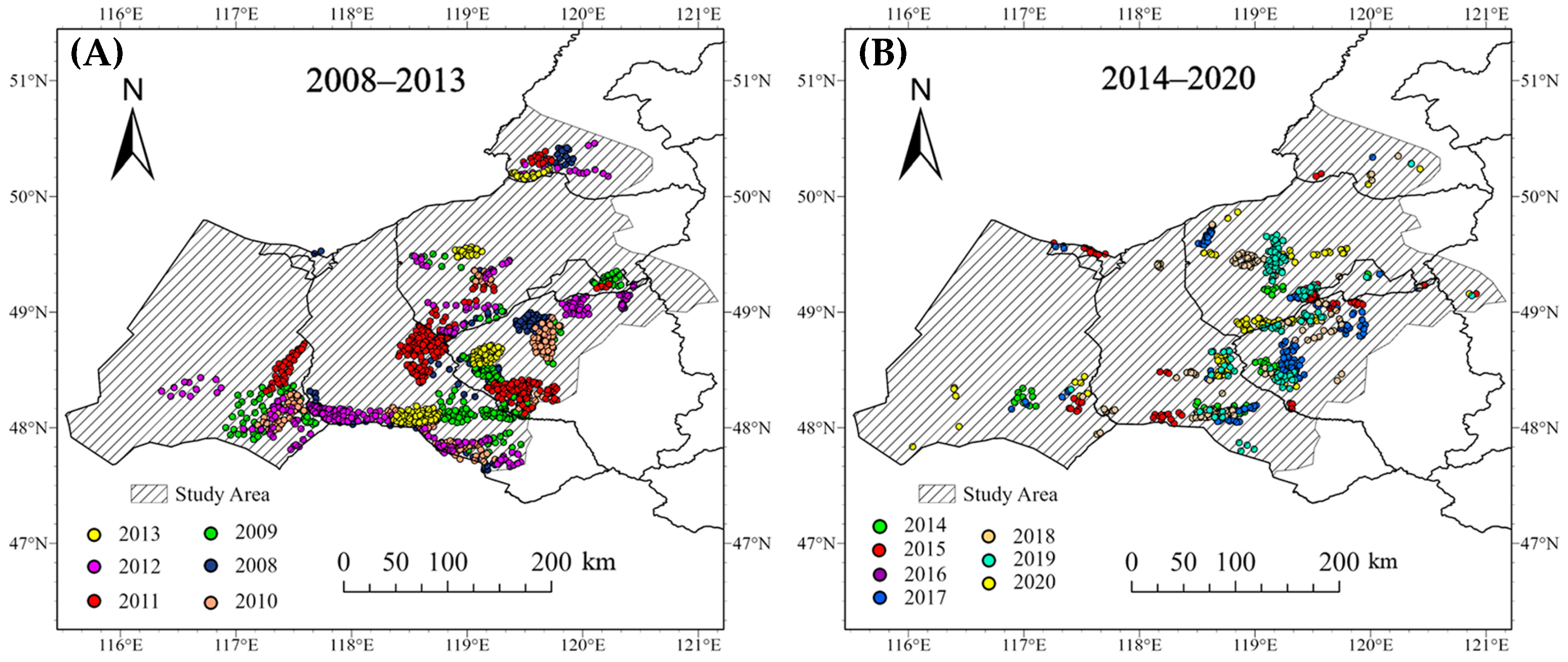
Firstly, foundational survey routes were established based on the occurrence time of dominant species from 2008 to 2020. After that, the Inner Mongolia Hulunbuir Grassland Station conducted comprehensive investigations in vegetation areas susceptible to grasshopper infestations by drawing on past work experience. The regions and locations affected by grasshopper disasters were documented during field surveys. Additionally, the extent of the disasters, the affected areas, the degree of damage caused, and the types of grasshoppers were reported. Finally, random sampling was performed in areas with suitable vegetation and soil, guided by the occurrence range of grasshoppers observed during the field surveys, in accordance with the national standard guideline for segmenting and monitoring inhabitable areas for locusts and grasshoppers in grasslands (GB/T 25875-2010) [45]. In order to preserve the aesthetic appeal, the representation is divided into two images, as illustrated in Figure 3.

2.3.2. Environmental Factors Based on Multisource Data

Building upon prior research by Guo [39], it has been established that meteorological, vegetation, soil, and topographic factors have distinct effects on the survival and breeding activities of grasshoppers. Considering the environmental factors at various developmental stages influencing grasshopper activities and the survival status of grasshopper eggs, a total of 27 factors were chosen each year, as shown in Table 1. Apart from the soil type and vegetation type, which are discrete variables, the rest of the factors are continuous variables.
This study was conducted using the Google Earth Engine (GEE). The average and minimum land surface temperatures of the four stages were extracted using the MOD11A1.061 data product. Precipitation data for the four developmental stages were obtained from the GPM v6 dataset, and soil moisture data for the overwintering, incubation, and spawning periods were sourced from the FLDAS: Famine Early Warning Systems Network (FEWS NET) Land Data Assimilation System dataset. To evaluate vegetation growth, the “NDVI” band of MOD13A2.061 data was used to calculate surface biomass in GEEusing a specific formula [46]:
A B = 26.38 × 10 3.8725 × N D V I
In this formula, e represents the natural logarithm base, and NDVI represents the corresponding Normalized Difference Vegetation Index.
Fractional Vegetation Coverage (FVC) is a crucial indicator for quantifying surface vegetation conditions and is also an important parameter for assessing the local environment [47]. The pixel-wise binary model, known for its simplicity and high accuracy, is widely applied in calculating vegetation coverage [48]. In this study, the “NDVI” band of MOD13A2.061 data was selected to calculate data for the four developmental stages, using the calculation formula shown in Equation (2) [49]:
F V C = S S s o i l S v e g S s o i l
In this equation, S s o i l represents the value corresponding to the cumulative 5th percentile of NDVI, while S v e g represents the value corresponding to the cumulative 95th percentile of NDVI. Furthermore, this study also considered the influence of soil salinity (SI) using MOD09A1.061 data to select remote sensing data in the red light band “sur_refl_b01” and the green light band “sur_refl_b04”, according to Equation (3) [50]. These bands represent the soil salinity conditions in the underground activity of grasshoppers, covering data for the overwintering and incubation periods.
S I = B g B r
In the above formula, B g represents the green band, and B r represents the red band.
The data acquisition and computation mentioned above were all carried out using GEE. The resolution of all factors was reprojected, masked, and resampled to 1 km. The series of MODIS products in version 6.1 was improved by undergoing various calibrations, comparing previous data.
Vegetation type and soil type data were acquired from a national database, which was updated in 2008, with a resolution of 1:1,000,000. These data comprehensively record the current plant communities and soil type classifications in China. Due to minor changes over several years, vegetation and soil type can be treated as static factors. Elevation data (DEM) were obtained from the GDEM V2 and V3 datasets available on the Geospatial Data Cloud (https://www.gscloud.cn/, accessed on 16 April 2023). GDEM V2 and V3 have higher accuracy than V1. The acquired DEM data were imported into ArcGIS, and the slope and aspect data of the study area were computed using toolbox tools. Afterwards, they were resampled to a 1 km resolution.

2.3.3. Selection of Environmental Factors

Based on the literature review, factors with strong collinearity exhibit correlation coefficients greater than 0.8 [51]. In this study, strong collinear variables were selected for their relevance based on their correlation magnitude and contribution to the model. The more influential variables were retained [25]. Additionally, Pearson correlation coefficients were used to assess the presence of collinearity among continuous variables. However, since calculating Pearson correlations for categorical variables is meaningless, soil and VT were not considered in this analysis. All factors were initially inputted into the model to observe their impact on the model’s response, using permutation importance as the evaluation criterion. The final selected factors were as follows: IP_LST_mean, OP_LST_mean, SP_LST_mean, EP_LST_mean, LST_IP_min, LST_SP_min, OP_pr_mean, IP_pr_mean, SP_pr_mean, EP_pr_mean, SPFVC, VT, OPmoisture, OPsal, soil, elevation, slope, and aspect.

2.4. Extraction of GPH Based on MaxEnt

2.4.1. Principles of MaxEnt

The Maximum Entropy Model (MaxEnt) was initially proposed by Phillips in 2006 [52]. MaxEnt is extensively applied in the field of species distribution prediction. Its concept originates from statistical mechanics, and its main function is to estimate the distribution of the target probability by finding the probability distribution with the maximum entropy. Maximum entropy is constrained by the available information about the target distribution, often referred to as features. These constraints consist of the empirical average values of the expected values for each feature. In models that consider all environmental factors, the outcome with the highest entropy and the most uniform distribution is selected for predicting species distribution. The entropy value can reflect the level of randomness in a model’s selection of unknown elements given known conditions. A higher entropy value implies a stronger level of randomness, making the model’s selection of unknown elements fair [53]. When MaxEnt is used exclusively for species distribution modeling, the pixels in the study area represent the area defined by the MaxEnt probability distribution. These pixels incorporate various features such as the climate, elevation, soil, vegetation, and other environmental variables. Once the model is given species distribution points and environmental variables, the entropy values of the random variable xi are computed for different potential outcomes based on the second law of thermodynamics. These computations are performed on a finite set X , which represents the set of pixels in the study area. The calculation of entropy values can be expressed as follows [52,54]:
H π ^ = x X π ^ x ln π ^ x
where π ^ x represents the species distribution probability values on the finite set X under m different potential outcomes X = x 1 , x 2 , x 3 , , x m , with m being the total number of possible outcomes for the discrete random variable X . The entropy values are non-negative. In practical applications, X can be understood as the set of pixels within the study area. For each feature in the environmental variables, it is defined as a set of known real values. MaxEnt calculates the empirical average for each feature. The MaxEnt distribution can be represented as a minimized Gibbs distribution:
π ~ ln q λ + j β j λ j
The possible distribution form (probability value) of each sample point is represented by q λ , which is known as the Gibbs distribution. β j represents the penalty term, and λ j represents the penalty weight. The first term above indicates omission, while the second term incorporates penalty weights. Consequently, the resulting MaxEnt output is more focused on minimizing penalty values and prioritizing the most important features. This makes the model less prone to overfitting. During model computation, it initiates from λ = ( 0 , , 0 ) and iteratively adjusts, making the regularized log-likelihood a convex function of the weights. So, local minima are absent, and convex optimization techniques can be used to ensure convergence to the global minimum for weight adjustment. In conclusion, the objective of the MaxEnt model is to approximate the joint probability distribution p of input x and output labels, thereby eliminating the need for missing data.
The MaxEnt model software used in this study was the version 3.4.3, which was downloaded from the American Museum of Natural History website (https://biodiversityinformatics.amnh.org/open_source/maxent, accessed on 27 April 2023). We used a random seed, which results in different selections in each run. Additionally, 70% of the dataset was used for training, while the remaining 30% was used for testing. The model was replicated 30 times for each year, and each time, points were selected using random bootstrap subsampling with replacement. Among the four output options provided by MaxEnt (Cloglog, logistic, cumulative, raw), the most interpretable option, logistic, was chosen as the format for the model’s predictions. Strictly speaking, logistic is not the original output of the MaxEnt model. The MaxEnt model often assigns very small raw values to each pixel, and the logistic output is a transformation of the original values. The conversion from raw values to logistic values can be expressed as follows [55]:
l o g i s t i c = c · r 1 + c · r
In this equation, c represents the entropy index in the maximum entropy distribution, and r represents the raw original value.

2.4.2. GPH Classification

To measure the likelihood and extent of grasshopper infestations in different areas of the study region, this study conducted suitability mapping and grading. The study used a 30 m uniform grid resolution to accurately represent changes in grassland caused by land cover changes, aligning with the resolution of the grassland. The specific steps included reclassifying the obtained land-use data to extract areas that only have grassland cover. Afterward, the model’s suitability layers were resampled to 30 m.
The classification of GPH employs a four-level partition scheme. Currently, there are various classification methods available for GPH. This study adopted the classification scheme proposed by Lu and Guo [39,40], who systematically classified suitability zones for grasshoppers in different regions of Inner Mongolia. Therefore, based on the existing classification scheme, GPH in the study area can be categorized as follows: logistic output values within the range of [0, 0.2) are classified as unsuitable, values within the range of (0.2, 0.5] are classified as less suitable, values within the range of (0.4, 0.7] are classified as moderately suitable, and values within the range of (0.7, 1] are classified as highly suitable.

2.5. Spatiotemporal Analysis of GPH

The code for the raster trend analysis method Sen-MK used in this paper is written in MATLAB R2022b. This code is based on the principles described below. The long-term raster detection method Sen-MK combines the Theil–Sen and Mann–Kendall test methods. This method is a non-parametric test that does not require the data to follow a normal distribution [56]. In fact, the Mann–Kendall method has some limitations. The trend test is consistently conducted in conjunction with autocorrelations [57]. The Theil-Sen method can strengthen the robustness of outliers. In long-term raster trend analyses, the Sen-MK trend analysis method is widely used. It involves two aspects: slope estimation and calculation of statistics. The formula is as follows:
β S e n = M e d i a n G j G i j i , j > i  
In this formula, G j and G i represent the layers corresponding to the j t h and i t h years in the time series ( j representing a later time than i ). M e d i a n (   ) denotes the median function. β S e n represents the median of all calculated slopes. β S e n > 0 implies an increasing trend in the time series; β S e n = 0 suggests no trend, indicating no change in the time series; β S e n < 0 indicates a decreasing trend in the time series. β S e n is very unlikely to be zero, so this would not usually be considered.
To quantify the magnitude of the declining trend, the MK method is employed to calculate the statistic Z . The statistic Z can indicate a downward or upward trend in the time series with a certain level of confidence. The steps of this method involve first calculating the test statistic S , which can be expressed using the following formula:
s g n θ = + 1 i f   θ > 0 0 i f   θ = 0 1 i f   θ < 0
S = i = 1 n 1 j = i + 1 n s g n G j G i
Here, n represents the length of the time series, and s g n ( θ ) is the sign function. The statistic Z is calculated as follows:
V a r S = n n 1 2 n + 5 18
Z = S 1 V a r S , i f S > 0 0 , i f S = 0 S + 1 V a r S , i f S < 0
This study employs a two-tailed trend test to determine the change trends:
Z Z 1 α 2  
According to the normal distribution table, when α = 0.05 , it means that at the significance level α = 0.05 , the null hypothesis is accepted, and the trend has passed the 95% confidence test. For Z1, the values 1.645 and 1.96 are used, corresponding to α = 0.1 and 0.05, indicating that the trend has passed the test at 90% and 95% confidence levels, respectively. Based on the Sen slope, this study categorizes trends into five levels: significant increase, slight increase, slight decrease, significant decrease, and unchanged, as shown in Table 2.

2.6. Analysis Process

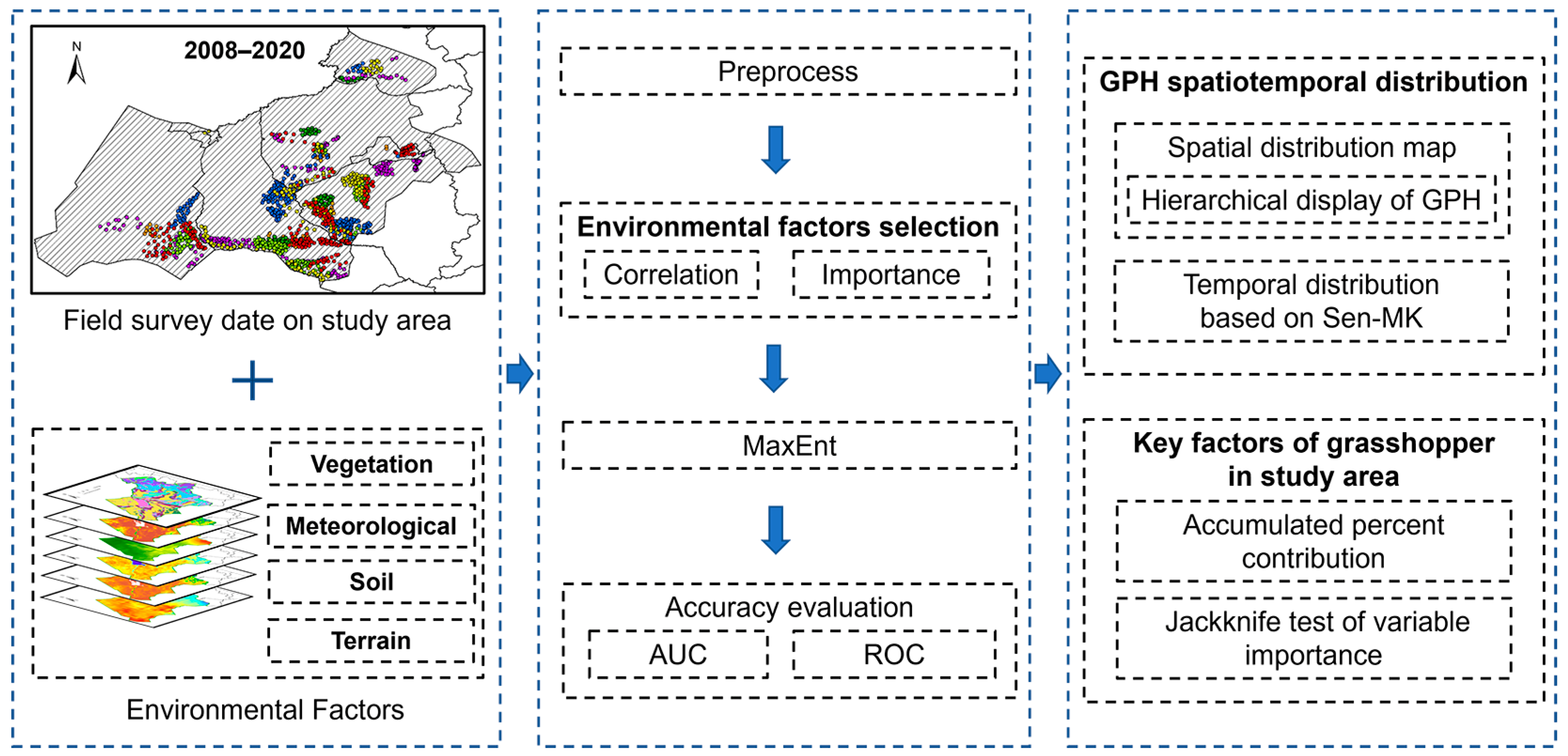
The analysis process is illustrated in Figure 4. Initially, relevant environmental variables were meticulously selected based on field survey data acquired within the designated study area and obtained from multiple resources. Subsequently, ArcGIS 10.6 software was utilized to implement a model tool for the batch processing of these environmental factors. This ensured that they had the same coordinate system and resolution, while simultaneously ensuring consistency in terms of grid cell dimensions. After that, a total of 18 significant influencing factors associated with the distribution of grasshoppers were identified through the use of Pearson correlation coefficients. Next, GPH was extracted using the MaxEnt model, and the performance of the model was assessed using ROC curves and the AUC metric. Following that, in conjunction with previous research findings, a classification was conducted to identify suitable habitat areas. Additionally, based on the model’s output, along with the Sen-MK method, a spatiotemporal distribution study of the study area was conducted. Lastly, a comprehensive analysis was conducted to extract the primary factors utilized in the distribution of grasshoppers.

3. Results

3.1. Accuracy Evaluation

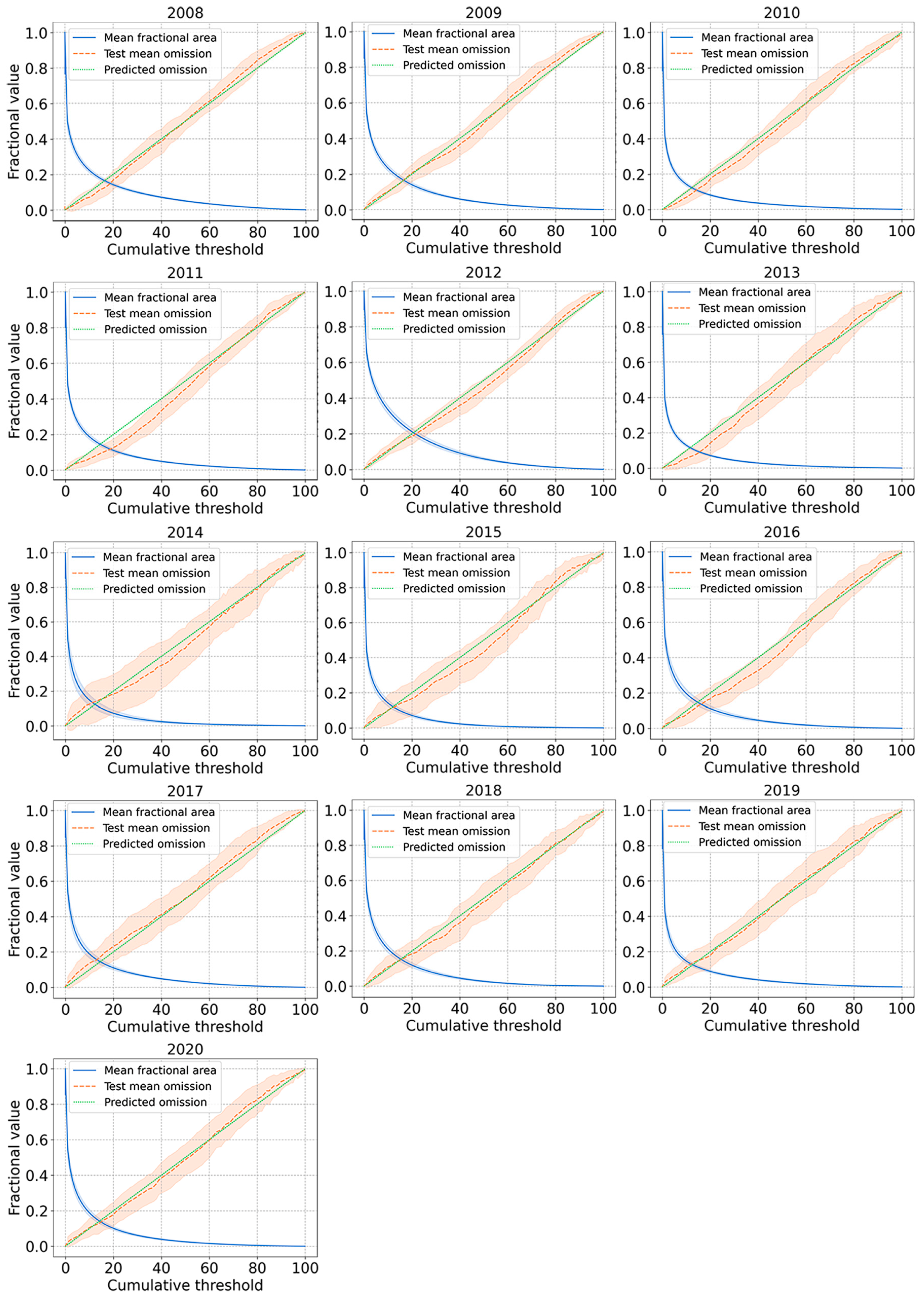
Figure 5 depicts the omission curve from 2008 to 2020. As fractional values increase, the corresponding cumulative threshold decreases. This indicates that higher logistic values result in lower model output probabilities. The omission rate can identify differences between models and evaluate whether there is overfitting. The orange curves represent the omission rates for the test dataset, while the corresponding green lines represent the predicted omission curves. Generally, as the cumulative threshold increases, the corresponding omission rate also increases. There should be a positive correlation between the two lines. The omission curves in the figure show that the omission rates for the test dataset and the predicted omission rates follow a similar trend. This indicates that the model construction is effective and overfitting is not observed. Moreover, there is no spatial autocorrelation among the modeling data [58].
The ROC curve, which stands for the Receiver Operating Characteristic curve, graphically represents the true negative rate on the x-axis and the true positive rate on the y-axis. In this study, the true negative rate refers to the accurate prediction of the absence of grasshopper distribution in the projected area. Conversely, the true negative rate refers to accurately predicting the grasshopper distribution in the projected area. Notably, in MaxEnt model computations, only the presence points of the species are utilized. Therefore, the true negative rate and true positive rate are expressed using 1-specificity (prediction score) and sensitivity (1-test set omission rate), respectively. ROC curves and the AUC (Area Under the Curve) are typically used together, with the AUC representing the area under the ROC curve. A larger AUC implies superior model performance [59]. Figure 6 visually represents the ROC curves for the 13-year test set, while Table 3 details the AUC results for 30 model computations in each corresponding year. The results confirm that the ROC curves consistently trended towards the upper left corner over the 13-year period, indicating improved model performance. Additionally, the AUC values range from 0.8456 to 0.9897, indicating commendable overall performance. This all signifies exceptional model performance levels.

3.2. The Spatial Distribution of GPH

For this study, the average logistic output of 30 models was chosen as the final predicted habitat for grasshoppers. Figure 7 illustrates the results of the classification of GPH for the years 2008 to 2020, spanning 13 years, in the study area. There are four suitability levels in the study area, with higher levels indicating a greater degree of harm. As indicated by these figures, the majority of the damage is concentrated in the central, southern, and northeastern regions of the study area. The highest suitability level is mainly distributed in the central region of the study area. In some years (2009, 2010, 2012), the highest degree of harm is predominantly concentrated in the southern region of the study area. Furthermore, there are also certain risks in the northern region, which were more pronounced in 2008.
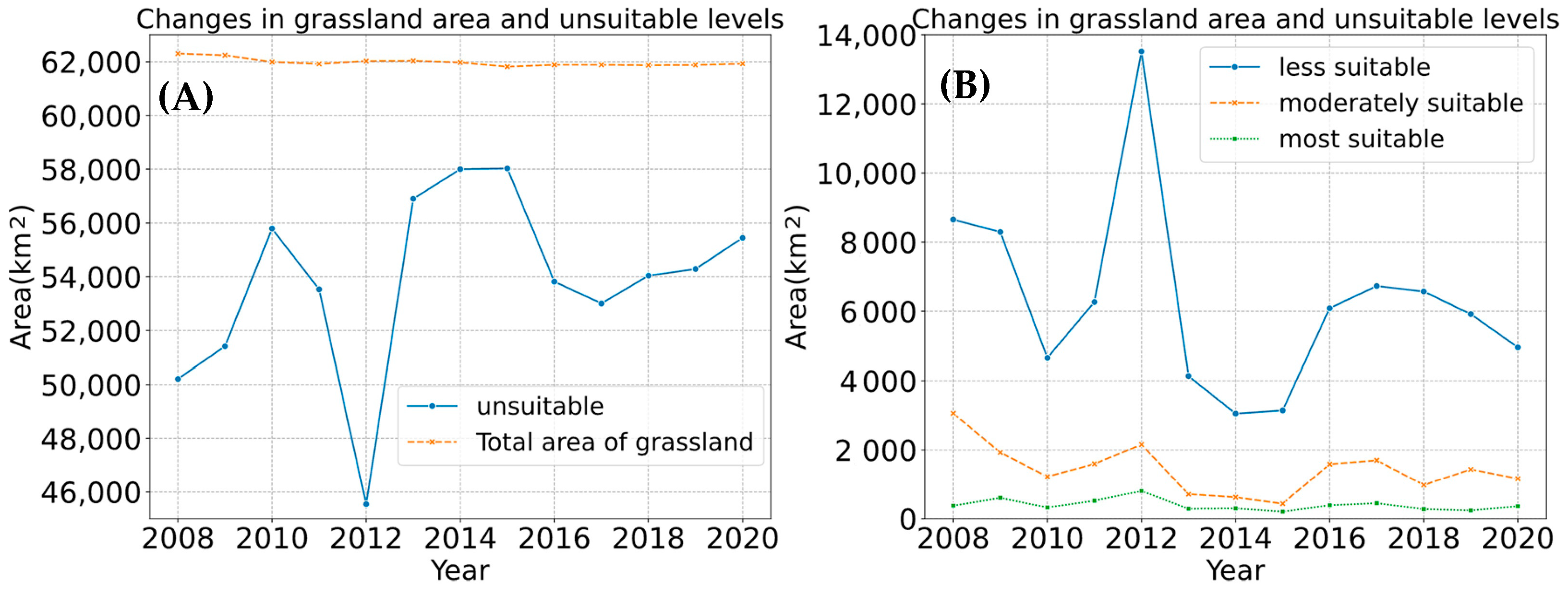
The area of suitable habitat was calculated at various levels for different years, and the changing trends can be observed in Figure 8. Over the 13 years, the area characterized as unsuitable is the largest, followed by the less suitable area, then the moderately suitable area, and finally the most suitable area, with the highest suitability. As the level of suitability increases, the corresponding area decreases accordingly, which is consistent with certain natural patterns. The grassland area remained relatively stable. The area of the unsuitable regions fluctuated between 50,000 km2 and 57,000 km2, reaching a peak of 58,029.59 km2 in 2015. Conversely, the less suitable area peaked in 2012, reaching 13,519.84 km2. The area of the moderately suitable level fluctuated during the study period from 2008 to 2010 and from 2012 to 2016: the largest area was 3061.89 km2 in 2008, and the smallest was 437.16 km2 in 2015. Furthermore, the area of highest suitability remained relatively stable over the 13-year period, with larger areas in 2009, 2011, and 2012, and smaller areas in the other years, all measuring below 500 km2. When comparing the suitability of different habitat areas, the unsuitable area was relatively smaller in 2012, while larger areas were observed in the other three categories. This indicates that 2012 experienced the most damage. In contrast, 2015 had a minimal impact, as evidenced by the larger unsuitable habitat area and smaller areas in the other categories.

3.3. The Temporal Variation in GPH

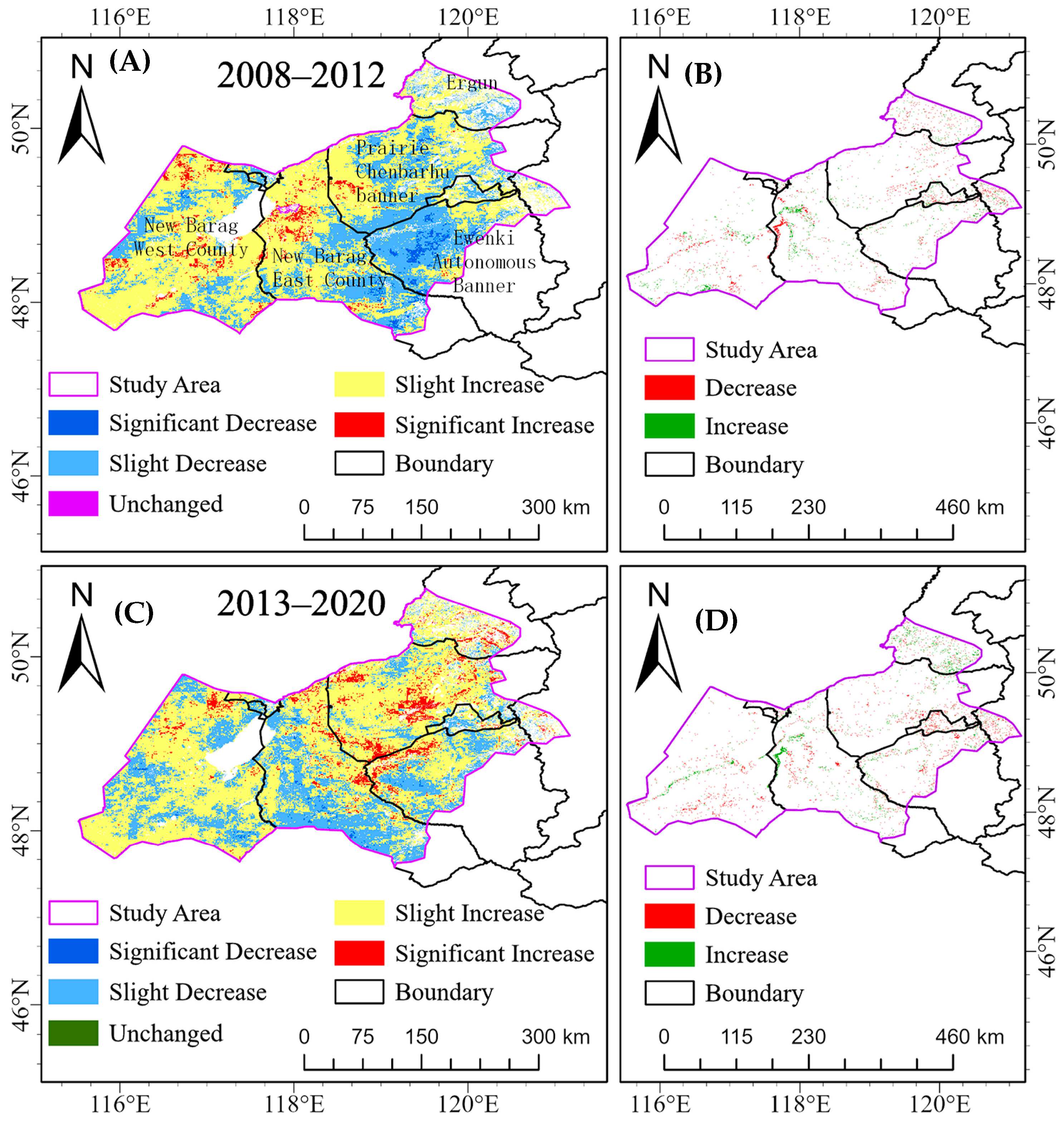
Based on the observed variations affected by grasshopper outbreaks, which indicate the highest severity being in 2012, this paper designates 2012 as a pivotal year. Consequently, trend tests were performed separately for the periods 2008 to 2012 and 2013 to 2020, using a two-segment trend test approach. In order to improve the accuracy of the analysis, two additional factors were taken into account when assessing the influence of environmental variables on annual outbreaks in GPH. Firstly, non-grassland areas were excluded before calculating. Secondly, we considered variations in the expansion and degradation of grasslands, as they can influence changes in habitat area. Given the absence of significant changes in the grassland over the 13-year period, the Raster Calculator tool in ArcGIS was utilized to compute the alterations in grassland between 2008 and 2012, as well as between 2013 and 2020. Finally, we merged the maps of the changing grassland areas to observe the fluctuations in GPH risks in different regions. The trend test results for the periods 2008–2012 and 2013–2020, along with the changes in the grassland, are shown in Figure 9.
Figure 9A illustrates trends from 2008 to 2012, showing slight increases and slight decreases as the main features. There were significant increases in New Barag East County and New Barag West County, while decreases are predominant in the Ewenki Autonomous Banner within the study area. This suggests that between 2008 and 2012, New Barag East County and New Barag West County experienced an increased risk of grasshopper outbreaks, while the risk in the Ewenki Autonomous Banner improved. It is noteworthy that in New Barag West County, some areas exhibit both decreases and increases in grassland (Figure 9B). This observation implies that the transformation of this region can be ascribed to alterations in the grasslands.
Figure 9C indicates that between 2013 and 2020, most regions demonstrate a slight increasing trend. Notably, the border area between the Ewenki Autonomous Banner and Chen Barag Banner, as well as New Barag West County and the northern part of New Barag East County, exhibit significant increasing trends. This suggests that over the 8-year period, these areas became more favorable for grasshopper outbreaks. In the southern part of New Barag East County, there was a small area, but a significant decreasing trend was observed, indicating effective measures in controlling infestations in that area. Additionally, changes in GPH are influenced by alterations in grassland, as shown in Figure 9D.

3.4. Key Factors of Grasshopper Outbreaks

The percentage contribution serves as a meaningful indicator of the significance of variables within the model. By evaluating their contributions, crucial factors for monitoring grasshopper outbreaks can be systematically identified. This paper conducted a dual analysis of these key factors to identify both the pivotal factors for different years and those that collectively play a comprehensive role.

3.4.1. Key Factors Per Year

Key factors were identified each year to represent grasshoppers based on their annual contributions. Following the methodology outlined in Wan, et al. [60], we considered factors with cumulative contributions surpassing 80% in the MaxEnt model as significant influencers for grasshopper monitoring. The specific key factors selected for each year are presented in Table 4.
The key factors for each year from 2008 to 2020 exhibit variability. However, an analysis of their contributions reveals that meteorological factors consistently account for the largest proportion, with rainfall being the most influential. Specifically, the variables EP_pr_mean and IP_pr_mean are identified as crucial factors influencing grasshopper outbreaks, potentially affecting their activity and egg hatching, respectively. LST also consistently proves to be a key factor throughout most years. Additionally, vegetation type (VT) consistently plays a significant role in annual grasshopper monitoring, while soil types also play a relatively important role. However, SPFVC, OPsal, and OPmoisture only serve as key factors in certain years, exerting a relatively minor influence compared to other factors. Among the topographic factors, only elevation in 2015 was identified as a key factor.
In summary, meteorological factors play the most crucial role in the activities of grasshoppers, with precipitation being the most significant. The vegetation is relatively crucial, and the vegetation type makes tremendous contributions. Soil factors, particularly the soil type, are slightly important, followed by the soil salinity index and soil moisture content. Topographic factors, represented by elevation in 2015, have the least overall impact in this study.

3.4.2. Key Factors Playing a Comprehensive Role in the 13 Years

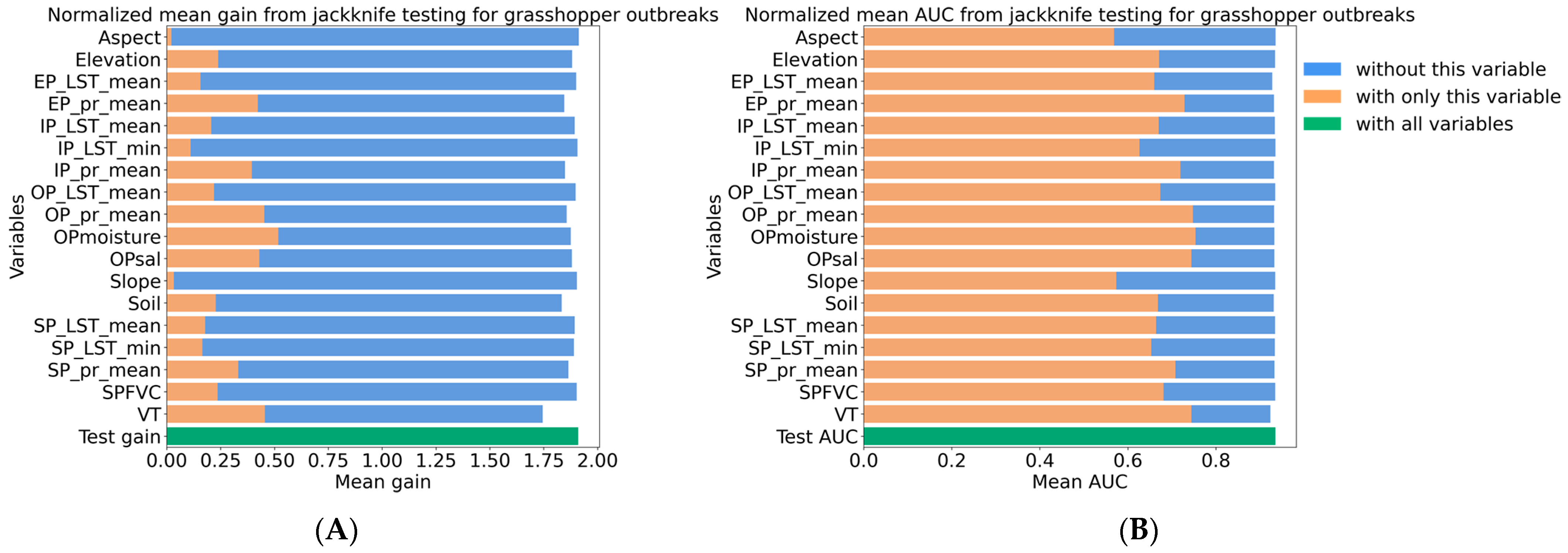
To comprehensively identify the factors that significantly impact grasshopper outbreaks in the research area, this study employed the jackknife test to calculate the model’s AUC value and normalized the training scores with one variable, without this variable, and with all variables. The selection criterion is based on the premise that using only one variable for modeling produces the highest normalized score and AUC, while not using this variable results in the lowest value. The results are depicted in Figure 10A,B. By considering the important factors annually and ensuring that their combined average contribution exceeds 80%, the top seven factors were selected as the key factors for GPH. The results indicate that the EP_pr_mean, IP_pr_mean, OP_pr_mean, OPmoisture, OPsal, VT, and soil type showed the highest improvements and the most significant variations. Consequently, these seven factors have been identified as key factors for the Hulunbuir grassland region from 2008 to 2020.

4. Discussion

This study focuses on the monitoring and analysis of the study area as a critical area for grasshopper infestations. Initially, the various developmental stages of grasshoppers were defined based on field survey data and the dominant species. Subsequently, we carefully selected and filtered four types of environmental factors, namely meteorological, vegetation, soil, and topographical, resulting in the selection of 18 factors. Utilizing the MaxEnt model, GPH was extracted with high accuracy and classified into four levels, thereby illustrating the risk of grasshopper infestation in the study region. Lastly, we conducted a comprehensive analysis of grasshopper disaster trends and key factors over the past 13 years. The research findings highlight that the method used is reasonably accurate within the study area. Comparing to previous research using the MaxEnt model to identify GPH in Hulunbuir [61], our study shows improved accuracy. This improvement primarily stems from dividing the study area to exclude regions where grasshopper occurrence is unlikely. The successful application of this method establishes a reliable benchmark for future grasshopper monitoring. Additionally, this paper analyzes GPH trends over a 13-year period and explores the potential link between changes in GPH and changes in grasslands. This provides scientific and theoretical support for preventing and controlling grasshopper outbreaks in high-risk areas of the Hulunbuir region.
Further analysis revealed the pivotal role of meteorological and vegetation factors, emphasizing the significance of these factors in monitoring and predicting grasshopper distribution. Meteorological factors, such as precipitation and temperature, directly impact the survival and reproduction of grasshoppers. On the other hand, vegetation factors, especially those associated with vegetation type, indirectly indicate the availability of food and habitat. These factors are crucial to the model, and it is important to exercise caution when dealing with resolution to avoid potential information loss, especially when resampling low-resolution data to a higher resolution. Future research should continuously improve the application of high-resolution data and regional-scale environmental factors to gain a more comprehensive understanding and effectively address grasshopper issues. This will improve the accuracy of monitoring and prevention efforts.

5. Conclusions

This study employed a comprehensive approach, examining meteorology, vegetation, soil, and topography, and leveraging the biological characteristics and distribution patterns of grasshoppers. The MaxEnt model was constructed to extract the distribution of grasshoppers using multiple data sources. Initially, 18 factors were selected based on interactions between the four environmental factors and grasshopper developmental characteristics. The results demonstrated the high accuracy of the MaxEnt model and revealed the absence of spatial autocorrelation issues. In the subsequent comprehensive analysis, meteorological factors emerged as the most crucial, followed by vegetation, soil, and topography. Specifically, precipitation and vegetation type were identified as the most significant environmental factors. Notably, factors such as the average precipitation during the eclosion period, the monthly precipitation during the incubation period, the average precipitation during the overwintering period, the soil moisture and salinity index during the overwintering period, the vegetation type, and the soil type play critical roles for GPH.
Spatial analysis and the Sen-MK test were used to detect the spatiotemporal distribution of GPH. The results from these indicate that the central, southern, and northeastern regions of the study area suffered the greatest damage. Specifically, New Barag West County and the Ewenki Autonomous Banner were severely impacted, especially in 2012. The year 2015 was shown to suffer minimal damage. From 2008 to 2012, New Barag East County and New Barag West County became more susceptible to grasshopper infestation, while the Ewenki Autonomous Banner showed improvement. Over an eight-year period (2013–2020), an analysis of the grasshopper outbreak trends revealed increasing vulnerability in specific regions. While most areas exhibited a slight increase, significant increases were observed in the Chen Barag Banner, the border region between the Ewenki Autonomous Banner and Chen Barag Banner, New Barag West County, and the northern portion of New Barag East County. Conversely, the southern part of New Barag West County exhibited a small but significant decreasing trend, indicating successful efforts to mitigate grasshopper outbreaks. These findings establish a scientific foundation for the monitoring and control of grasshoppers. Future research should focus on refining the application of high-resolution data and regional-scale environmental factors to better address grasshopper-related issues.

Author Contributions

Conceptualization, Y.Z. and Y.D.; methodology, Y.Z., Y.D., W.H. and J.G.; validation, Y.Z.; formal analysis, Y.Z. and J.G.; investigation, N.W. and X.D.; resources, N.W. and X.D.; writing—original draft preparation, Y.Z.; writing—review and editing, Y.Z., Y.D., W.H., J.G., N.W. and X.D.; visualization, Y.Z.; supervision, Y.D. and W.H.; project administration, W.H.; funding acquisition, Y.D. All authors have read and agreed to the published version of the manuscript.

Funding

The work was supported by the National Key R & D Program of China (2022YFD140110X), Alliance of International Science Organizations (Grant No. ANSO-CR-KP-2021-06), the Project of Northern Agriculture and Livestock Husbandry Technical Innovation Center, Chinese Academy of Agricultural Sciences (BFGJ2022007), SINO- EU Dragon 5 proposal: Application Of Sino-Eu Optical Data Into Agronomic Models To Predict Crop Performance And To Monitor And Forecast Crop Pests And Diseases (ID 57457) and The APC was funded by GEO-PDRS: Global Vegetation Pest and Disease Dynamic Remote Sensing Monitoring and Forecasting (2023-2025).

Data Availability Statement

The grasshopper data are not publicly available because the data needs to be used in future work. Land surface temperatures is avaiable at https://developers.google.com/earth-engine/datasets/catalog/MODIS_061_MOD11A2, accessed on 15 April 2023. Surface biomass and Fractional Vegetation Coverage are avaiable at https://developers.google.com/earth-engine/datasets/catalog/MODIS_061_MOD13A2, accessed on 16 April 2023. Soil salinity is avaiable at https://developers.google.cn/earth-engine/datasets/catalog/MODIS_061_MOD09A1, accessed on 16 April 2023. Precipitation is avaiable at https://developers.google.cn/earth-engine/datasets/catalog/NASA_GPM_L3_IMERG_V06?hl=en, accessed on 16 April 2023. Vegetation Type and Soil Type are obtained from the Chinese Academy of Sciences, they are not supported for public disclosure. The elevation is available from Geospatial Data Cloud (https://www.gscloud.cn/, accessed on 16 April 2023).

Conflicts of Interest

The authors declare no conflicts of interest.

References

  1. Zhang, L.; Lecoq, M.; Latchininsky, A.; Hunter, D. Locust and Grasshopper Management. Annu. Rev. Entomol. 2019, 64, 15–34. [Google Scholar] [CrossRef]
  2. Hong, J.; Du, G.-l.; Wang, G.-J. The Occurring and Control Situation of Grasshopper in the Grassland of China (Review). Acta Agrestia Sin. 2014, 22, 929–934. [Google Scholar] [CrossRef]
  3. Cullen, D.A.; Cease, A.J.; Latchininsky, A.V.; Ayali, A.; Berry, K.; Buhl, J.; De Keyser, R.; Foquet, B.; Hadrich, J.C.; Matheson, T.; et al. Chapter Seven—From Molecules to Management: Mechanisms and Consequences of Locust Phase Polyphenism. In Advances in Insect Physiology; Verlinden, H., Ed.; Academic Press: Cambridge, MA, USA, 2017; Volume 53, pp. 167–285. [Google Scholar]
  4. Pener, M.P.; Simpson, S.J. Locust Phase Polyphenism: An Update. In Advances in Insect Physiology; Simpson, S.J., Pener, M.P., Eds.; Academic Press: Cambridge, MA, USA, 2009; Volume 36, pp. 1–272. [Google Scholar]
  5. Song, H.; Mariño-Pérez, R.; Woller, D.A.; Cigliano, M.M. Evolution, Diversification, and Biogeography of Grasshoppers (Orthoptera: Acrididae). Insect Syst. Divers. 2018, 2, 3. [Google Scholar] [CrossRef]
  6. Wegier, A.; Alavez, V.; Pérez-López, J.; Calzada, L.; Cerritos, R. Beef or grasshopper hamburgers: The ecological implications of choosing one over the other. Basic Appl. Ecol. 2018, 26, 89–100. [Google Scholar] [CrossRef]
  7. Li, L.; Zhao, C.; Zhao, X.; Wang, D.; Li, Y. Pattern of plant communities’ influence to grasshopper abundance distribution in heterogeneous landscapes at the upper reaches of Heihe River, Qilian Mountains, China. Environ. Sci. Pollut. Res. 2022, 29, 13177–13187. [Google Scholar] [CrossRef] [PubMed]
  8. Huang, W.; Dong, Y.; Zhao, L.; Geng, Y.; Ruan, C.; Zhang, B.; Sun, Z.; Zhang, S.; Ye, H.; Wang, K. Review of locust remote sensing monitoring and early warning. J. Remote Sens. 2020, 24, 1270–1279. [Google Scholar] [CrossRef]
  9. Dong, Y.; Xu, F.; Liu, L.; Du, X.; Ren, B.; Guo, A.; Geng, Y.; Ruan, C.; Ye, H.; Huang, W.; et al. Automatic System for Crop Pest and Disease Dynamic Monitoring and Early Forecasting. IEEE J. Sel. Top. Appl. Earth Obs. Remote Sens. 2020, 13, 4410–4418. [Google Scholar] [CrossRef]
  10. Elith, J.; Leathwick, J.R. Species Distribution Models: Ecological Explanation and Prediction Across Space and Time. Annu. Rev. Ecol. Evol. Syst. 2009, 40, 677–697. [Google Scholar] [CrossRef]
  11. Kistner-Thomas, E.; Kumar, S.; Jech, L.; Woller, D.A. Modeling Rangeland Grasshopper (Orthoptera: Acrididae) Population Density Using a Landscape-Level Predictive Mapping Approach. J. Econ. Entomol. 2021, 114, 1557–1567. [Google Scholar] [CrossRef]
  12. Ochieng’, V.; Rwomushana, I.; Ong’amo, G.; Ndegwa, P.; Kamau, S.; Makale, F.; Chacha, D.; Gadhia, K.; Akiri, M. Optimum Flight Height for the Control of Desert Locusts Using Unmanned Aerial Vehicles (UAV). Drones 2023, 7, 233. [Google Scholar] [CrossRef]
  13. Olfert, O.; Weiss, R.M.; Giffen, D.; Vankosky, M.A. Modeling Ecological Dynamics of a Major Agricultural Pest Insect (Melanoplus sanguinipes; Orthoptera: Acrididae): A Cohort-Based Approach Incorporating the Effects of Weather on Grasshopper Development and Abundance. J. Econ. Entomol. 2020, 114, 122–130. [Google Scholar] [CrossRef]
  14. Klein, I.; Oppelt, N.; Kuenzer, C. Application of Remote Sensing Data for Locust Research and Management—A Review. Insects 2021, 12, 233. [Google Scholar] [CrossRef]
  15. Abd El-Ghany, N.M.; Abd El-Aziz, S.E.; Marei, S.S. A review: Application of remote sensing as a promising strategy for insect pests and diseases management. Environ. Sci. Pollut. Res. 2020, 27, 33503–33515. [Google Scholar] [CrossRef]
  16. Bai, J.; Hou, P.; Zhao, Y.; Xv, H.; Zhang, B. Research progress of species habitat suitability models and their verification. Chin. J. Ecol. 2022, 41, 1423–1432. [Google Scholar] [CrossRef]
  17. Ju, X.; Lin, J.; Wu, J.; Chen, J.; Guan, J.; Li, M.; Zheng, J. Prediction of potential living area of typical locusts in Xinjiang based on species distribution model. Acta Ecol. Sin. 2022, 42, 8605–8617. [Google Scholar] [CrossRef]
  18. Sun, Z.; Ye, H.; Huang, W.; Qimuge, E.; Bai, H.; Nie, C.; Lu, L.; Qian, B.; Wu, B. Assessment on Potential Suitable Habitats of the Grasshopper Oedaleus decorus asiaticus in North China based on MaxEnt Modeling and Remote Sensing Data. Insects 2023, 14, 138. [Google Scholar] [CrossRef] [PubMed]
  19. Norberg, A.; Abrego, N.; Blanchet, F.G.; Adler, F.R.; Anderson, B.J.; Anttila, J.V.; Araújo, M.B.; Dallas, T.A.; Dunson, D.B.; Elith, J.; et al. A comprehensive evaluation of predictive performance of 33 species distribution models at species and community levels. Ecol. Monogr. 2019, 89, e01370. [Google Scholar] [CrossRef]
  20. Xu, D.; Zhuo, Z.; Wang, R.; Ye, M.; Pu, B. Modeling the distribution of Zanthoxylum armatum in China with MaxEnt modeling. Glob. Ecol. Conserv. 2019, 19, e00691. [Google Scholar] [CrossRef]
  21. Yan, H.; Feng, L.; Zhao, Y.; Feng, L.; Wu, D.; Zhu, C. Prediction of the spatial distribution of Alternanthera philoxeroides in China based on ArcGIS and MaxEnt. Glob. Ecol. Conserv. 2020, 21, e00856. [Google Scholar] [CrossRef]
  22. Sivyer, L.; Morgan-Richards, M.; Koot, E.; Trewick, S.A. Anthropogenic cause of range shifts and gene flow between two grasshopper species revealed by environmental modelling, geometric morphometrics and population genetics. Insect Conserv. Divers. 2018, 11, 415–434. [Google Scholar] [CrossRef]
  23. Yang, H.; Zheng, J.; Wu, X.; Mu, C.; Lin, J.; Xu, Z. Prediction of Potential Distribution Area of Gomphocerus sibiric in China Based on the MaxEnt Model. Xinjiang Agric. Sci. 2016, 53, 43–50. [Google Scholar]
  24. Flores, R.C.; Ponce-Reye, R.; Rojas-García4, F. Exploiting a pest insect species Sphenarium purpurascens for human consumption: Ecological, social, and economic repercussions. J. Insects Food Feed 2015, 1, 75–84. [Google Scholar] [CrossRef]
  25. Adu-Acheampong, S.; Samways, M.J.; Landmann, T.; Kyerematen, R.; Minkah, R.; Mukundamago, M.; Moshobane, C.M. Endemic grasshopper species distribution in an agro-natural landscape of the Cape Floristic Region, South Africa. Ecol. Eng. 2017, 105, 133–140. [Google Scholar] [CrossRef]
  26. Sun, Z.; Hu, Z.; Ye, H.; Huang, W.; Erden, Q.; Zhang, Y. Application of MaxEnt and Remote Sensing Technology in Grassland Locust Disaster Risk Monitoring: An Example from the Agricultural Heritage Systems of East Ujimqin Banner. J. Ecol. Rural Environ. 2022, 38, 1265–1272. (In Chinese) [Google Scholar] [CrossRef]
  27. Klein, I.; Uereyen, S.; Eisfelder, C.; Pankov, V.; Oppelt, N.; Kuenzer, C. Application of geospatial and remote sensing data to support locust management. Int. J. Appl. Earth Obs. Geoinf. 2023, 117, 103212. [Google Scholar] [CrossRef]
  28. Li, J.; Liu, Q.; Liu, P. Spatio-temporal changes and driving forces of fraction of vegetation coverage in Hulunbuir (1998-2018). Acta Ecol. Sin. 2022, 42, 220–235. [Google Scholar] [CrossRef]
  29. Zhou, D.; Zhao, X.; Hu, H.; Shen, H.; Fang, J. Long-term vegetation changes in the four mega-sandy lands in Inner Mongolia, China. Landsc. Ecol. 2015, 30, 1613–1626. [Google Scholar] [CrossRef]
  30. Yunxiang, C.; Kamijo, T.; Tsubo, M.; Nakamura, T. Phytosociology of Hulunbeier grassland vegetation in Inner Mongolia, China. Phytocoenologia 2013, 43, 41–51. [Google Scholar] [CrossRef]
  31. Branson, D.H.; Joern, A.; Sword, G.A. Sustainable Management of Insect Herbivores in Grassland Ecosystems: New Perspectives in Grasshopper Control. BioScience 2006, 56, 743–755. [Google Scholar] [CrossRef]
  32. Chudzik, P.; Mitchell, A.; Alkaseem, M.; Wu, Y.; Fang, S.; Hudaib, T.; Pearson, S.; Al-Diri, B. Mobile Real-Time Grasshopper Detection and Data Aggregation Framework. Sci. Rep. 2020, 10, 1150. [Google Scholar] [CrossRef]
  33. Lockwood, J.A.; Hong-Chang, L.; Dodd, J.L.; Williams, S.E. Comparison of Grasshopper (Orthoptera: Acrididae) Ecology on the Grasslands of the Asian Steppe in Inner Mongolia and the Great Plains of North America. J. Orthoptera Res. 1994, 2, 4–14. [Google Scholar] [CrossRef]
  34. Wang, L.; Zhou, Q. Discussion on the Development of Physical Method in Locust Disaster-controlling and its Prospect. J. Anhui Agric. Sci. 2008, 36, 4. [Google Scholar]
  35. Shan, Y.; Ji, Y.; Li, S.; Ma, C.; Tu, X.; Wang, J.; Wei, J.; Zhang, Z.; Xv, C. Control of Locusts in Different Grasslands by Metarhizium anisopliae. Chin. J. Biol. Control 2021, 37, 946–955. [Google Scholar] [CrossRef]
  36. Zhao, C.; Li, L.; Wang, D.; Yin, C.; Sheng, Y. Analysis on grasshopper spatial heterogeneity and pattern of natural grass in upper reaches of Heihe. Acta Ecologica Sinica 2012, 32, 4166–4172. [Google Scholar] [CrossRef]
  37. Zhu, Y.; Ma, Q.; Zhong, Z.; Jiang, M.; Bakker, E.S.; Harvey, J.A.; Veen, G.F.; Chen, C.; Wang, D. Contrasting effects of nitrogen fertiliser application on the performance of closely related grasshoppers through changes in plant nutrient concentrations. Ecol. Entomol. 2023, 48, 347–357. [Google Scholar] [CrossRef]
  38. Lecoq, M. Integrated Pest Management for Locusts and Grasshoppers: Are Alternatives to Chemical Pesticides Credible? J. Orthoptera Res. 2010, 19, 131–132. [Google Scholar] [CrossRef]
  39. Guo, J.; Lu, L.; Dong, Y.; Huang, W.; Zhang, B.; Du, B.; Ding, C.; Ye, H.; Wang, K.; Huang, Y.; et al. Spatiotemporal Distribution and Main Influencing Factors of Grasshopper Potential Habitats in Two Steppe Types of Inner Mongolia, China. Remote Sens. 2023, 15, 866. [Google Scholar] [CrossRef]
  40. Lu, L.; Kong, W.; Eerdengqimuge; Ye, H.; Sun, Z.; Wang, N.; Du, B.; Zhou, Y.; Weijun; Huang, W. Detecting Key Factors of Grasshopper Occurrence in Typical Steppe and Meadow Steppe by Integrating Machine Learning Model and Remote Sensing Data. Insects 2022, 13, 894. [Google Scholar] [CrossRef] [PubMed]
  41. Wei, S.; Liu, X.; McNeill, M.R.; Wang, Y.; Sun, W.; Tu, X.; Wang, G.; Ban, L.; Zhang, Z.; Zhang, R. Identification of spatial distribution and drivers for grasshopper populations based on geographic detectors. Ecol. Indic. 2023, 154, 110500. [Google Scholar] [CrossRef]
  42. Piou, C.; Gay, P.E.; Benahi, A.S.; Babah Ebbe, M.A.O.; Chihrane, J.; Ghaout, S.; Cisse, S.; Diakite, F.; Lazar, M.; Cressman, K.; et al. Soil moisture from remote sensing to forecast desert locust presence. J. Appl. Ecol. 2019, 56, 966–975. [Google Scholar] [CrossRef]
  43. Wang, Y.; Li, S.; Du, G.; Hu, G.; Zhang, Y.; Tu, X.; Zhang, Z. An analysis of the possible migration routes of Oedaleus decorus asiaticus Bey-Bienko (Orthoptera: Acrididae) from Mongolia to China. Insects 2022, 13, 72. [Google Scholar] [CrossRef]
  44. Huang, X.; Ma, J.; Qin, X.; Tu, X.; Cao, G.; Wang, G.; Nong, X.; Zhang, Z. Biology, physiology and gene expression of grasshopper Oedaleus asiaticus exposed to diet stress from plant secondary compounds. Sci. Rep. 2017, 7, 8655. [Google Scholar] [CrossRef] [PubMed]
  45. GB/T 25875-2010; Guideline for Segmenting and Monitoring the Inhabitable areas of for Locusts and Grasshoppers in Grasslands. Standardization Administration of the People’s Republic of China: Beijing, China, 2011.
  46. Ma, W.; Fang, J.; Yang, Y.; Mohammat, A. Biomass carbon stocks and their changes in northern China’s grasslands during 1982–2006. Sci. China Life Sci. 2010, 53, 841–850. [Google Scholar] [CrossRef] [PubMed]
  47. Xing, C.-R.; Feng, Y.-G.; Yang, G.; Wang, P.; Huang, W.-J. Method of Estimating Vegetation Coverage Based on Remote Sensing. Remote Sens. Technol. Appl. 2012, 24, 849–854. [Google Scholar] [CrossRef]
  48. Jia, K.; Yao, Y.; Wei, X.; Gaoi, S.; Jiang, B.; Zhao, X. A Review on Fractional Vegetation Cover Estimation Using Remote Sensing. Adv. Earth Sci. 2013, 28, 774–782. [Google Scholar] [CrossRef]
  49. Tu, Y.; Jia, K.; Wei, X.; Yao, Y.; Xia, M.; Zhang, X.; Jiang, B. A time-efficient fractional vegetation cover estimation method using the dynamic vegetation growth information from time series Glass FVC product. IEEE Geosci. Remote Sens. Lett. 2019, 17, 1672–1676. [Google Scholar] [CrossRef]
  50. Wang, F.; Chen, X.; Luo, G.; Ding, J.; Chen, X. Detecting soil salinity with arid fraction integrated index and salinity index in feature space using Landsat TM imagery. J. Arid Land 2013, 5, 340–353. [Google Scholar] [CrossRef]
  51. Bujang, M.A. A simplified guide to determination of sample size requirements for estimating the value of intraclass correlation coefficient: A review. Arch. Orofac. Sci. 2017, 12, 1–11. [Google Scholar]
  52. Phillips, S.J.; Anderson, R.P.; Schapire, R.E. Maximum entropy modeling of species geographic distributions. Ecol. Model. 2006, 190, 231–259. [Google Scholar] [CrossRef]
  53. Kaky, E.; Nolan, V.; Alatawi, A.; Gilbert, F. A comparison between Ensemble and MaxEnt species distribution modelling approaches for conservation: A case study with Egyptian medicinal plants. Ecol. Inform. 2020, 60, 101150. [Google Scholar] [CrossRef]
  54. Elith, J.; Graham, C.H.; Anderson, R.P.; Dudík, M.; Ferrier, S.; Guisan, A.; Hijmans, R.J.; Huettmann, F.; Leathwick, J.R.; Lehmann, A.; et al. Novel methods improve prediction of species’ distributions from occurrence data. Ecography 2006, 29, 129–151. [Google Scholar] [CrossRef]
  55. Phillips, S.J.; Dudík, M. Modeling of species distributions with Maxent: New extensions and a comprehensive evaluation. Ecography 2008, 31, 161–175. [Google Scholar] [CrossRef]
  56. Gowthaman, T.; Kumar, S.; Bhattacharyya, B. Detecting air pollutants trends using Mann-Kendall tests and Sen’s slope estimates. Environ. Conserv. J. 2023, 24, 157–166. [Google Scholar] [CrossRef]
  57. Liu, S.; Xie, Y.; Fang, H.; Du, H.; Xu, P. Trend Test for Hydrological and Climatic Time Series Considering the Interaction of Trend and Autocorrelations. Water 2022, 14, 3006. [Google Scholar] [CrossRef]
  58. Shcheglovitova, M.; Anderson, R.P. Estimating optimal complexity for ecological niche models: A jackknife approach for species with small sample sizes. Ecol. Model. 2013, 269, 9–17. [Google Scholar] [CrossRef]
  59. Yang, Z.; Xu, Q.; Bao, S.; Cao, X.; Huang, Q. Learning With Multiclass AUC: Theory and Algorithms. IEEE Trans. Pattern Anal. Mach. Intell. 2022, 44, 7747–7763. [Google Scholar] [CrossRef] [PubMed]
  60. Wan, G.-Z.; Wang, L.; Jin, L.; Chen, J. Evaluation of environmental factors affecting the quality of Codonopsis pilosula based on chromatographic fingerprint and MaxEnt model. Ind. Crops Prod. 2021, 170, 113783. [Google Scholar] [CrossRef]
  61. Du, B.; Wei, J.; Lin, K.; Lu, L.; Ding, X.; Ye, H.; Huang, W.; Wang, N. Spatial and Temporal Variability of Grassland Grasshopper Habitat Suitability and Its Main Influencing Factors. Remote Sens. 2022, 14, 3910. [Google Scholar] [CrossRef]
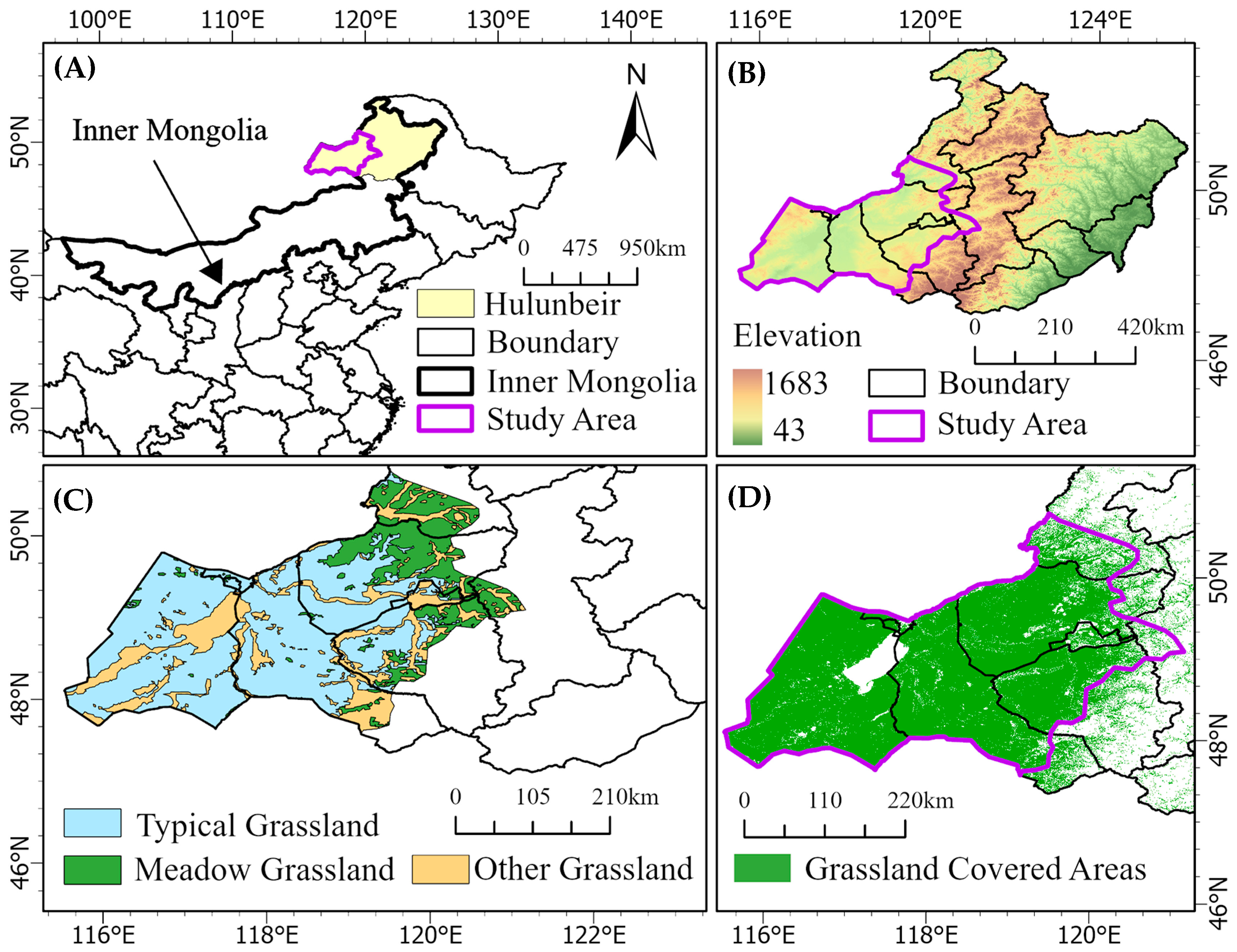
Figure 1. General situation of the study region. (A) The research area is situated in the eastern region of Hulunbuir. (B) The terrain conditions in the research area. (C) The grassland types in the study area mainly include meadow grassland, typical grassland, and others. (D) Distribution of grasslands in the study area.
Remotesensing 16 00746 g001
Figure 2. Environmental factors theoretically affecting grasshopper occurrence. Different factors change during each of the four periods, while the static factors in the center of the figure remain consistent throughout the whole year.
Remotesensing 16 00746 g002
Figure 3. Annual distribution of occurrence points. (A) Distribution of occurrence points from 2008 to 2013; each different year has a different color. (B) Distribution of occurrence points from 2014 to 2020.
Remotesensing 16 00746 g003
Figure 4. Analysis process, including selecting factors, MaxEnt modeling, accuracy evaluation, spatiotemporal distribution analysis, and judging key factors of grasshoppers in the study area.
Remotesensing 16 00746 g004
Figure 5. Omission curves representing 2008 to 2020, respectively. The blue line represents trends in the fractional values. The orange and green lines indicate the mean test omission and predicted omission. The shadow of the corresponding color represents the mean value ± one standard deviation of the model’s calculation results. The similar trends indicate good performance.
Remotesensing 16 00746 g005
Figure 6. ROC curves representing 2008 to 2020. The blue curves represent the results of adding or subtracting one standard deviation from the average after 30 repeated operations. The yellow curves represent the theoretical outputs of random operations. The blue shadow represents the mean value ± one standard deviation of the model’s calculation results.
Remotesensing 16 00746 g006
Figure 7. Annual GPH distribution. The red color represents the most suitable area. The yellow color represents areas that are less suitable. The orange color represents moderately suitable areas, while the green color represents unsuitable areas. The level of damage decreases sequentially.
Remotesensing 16 00746 g007
Figure 8. Changes in different areas from 2008 to 2020. (A) The orange line represents the changes in the total area of grassland, while the blue line represents the unsuitable area. (B) The blue line represents the less suitable area, the yellow line represents the moderately suitable area, and the green line represents the most suitable area.
Remotesensing 16 00746 g008
Figure 9. (A) Each color represents a different trend from 2008 to 2012. (B) The red area and green area represent the decrease and increase in grassland from 2008 to 2012. (C) Different colors represent distinct trends from 2013 to 2020. (D) The red area represents the decrease in grassland from 2013 to 2020, while the green area represents the increase.
Remotesensing 16 00746 g009
Figure 10. Normalized mean values from jackknife testing for grasshopper outbreaks. (A) This figure shows the testing gain without each variable, with only that variable, and with all variables, respectively. (B) This figure shows the AUC gain without each variable, with only that variable, and with all variables, respectively.
Remotesensing 16 00746 g010
Table 1. The environmental factors. The table outlines the source data, stage, symbol, and related resolution. There are 27 factors in total.
CategoryFactorsDevelopment StageSymbolData SourceResolution
MeteorologyAverage LSTOverwinteringLST_OP_meanMOD11A11 km
IncubationLST_IP_mean
EclosionLST_EP_mean
SpawningLST_SP_mean
Minimum LSTOverwinteringLST_IP_minMOD11A11 km
IncubationLST_IP_min
EclosionLST_EP_min
SpawningLST_SP_min
PrecipitationOverwinteringOP_pr_meanGPM11,132 m
IncubationIP_pr_mean
EclosionEP_ pr_mean
SpawningSP_ pr_mean
VegetationAboveground BiomassEclosionEPbioMOD09A1500 m
SpawningSPbio
Fractional Vegetation CoverIncubationIPFVCMOD13A21 km
EclosionEPFVC
SpawningSPFVC
Vegetation TypeStatic FactorVTChinese Academy of Sciences
SoilSoil MoistureOverwinteringSPmoistureFLDAS11,132 m
IncubationOPmoisture
SpawningIPmoisture
Soil SalinityOverwinteringIPsalMOD13A21 km
IncubationOPsal
Soil TypeStatic FactorSoilChinese Academy of Sciences1 km
TopographicElevationStatic FactorElevationGDEM V2/330 m
SlopeStatic FactorSlopeCalculation in ArcGIS
Slope AspectStatic FactorAspectCalculation in ArcGIS
Table 2. Trend level inspection classification.
Sen Slope Statistic   Z Trend Level
β S e n > 0 | Z | > 1.96significant increase
β S e n > 01.645 < | Z | < 1.96slight increase
β S e n < 01.645 < | Z | < 1.96slight decrease
β S e n < 0 | Z | > 1.96significant decrease
β S e n < 0, β S e n > 0 | Z | < 1.645unchanged
Table 3. AUC from 2008 to 2020. From 2008 to 2020, the model performance has been categorized into five levels: excellent (AUC between 0.9 and 1.0), good (AUC between 0.8 and 0.9), common (AUC between 0.7 and 0.8), bad (AUC between 0.6 and 0.7), and failed (AUC lower than 0.6).
YearExcellent (0.9, 1.0]Good (0.8, 0.9]Common (0.7, 0.8]Bad (0.6, 0.7]Failed ≤ 0.6Average AUCRange
20082910000.9190.892–0.946
20092820000.9120.889–0.941
20103000000.9550.942–0.972
20113000000.9420.907–0.965
20123270000.8830.853–0.911
20133000000.9620.922–0.979
20142730000.9440.860–0.990
20152910000.9530.887–0.982
20162910000.9340.892–0.969
201720100000.9120.846–0.948
20182640000.9280.881–0.965
20192910000.9350.888–0.966
20202640000.9670.880–0.958
Table 4. The key factors selected per year. The number of factors varies each year. Bold factors indicate their occurrence in many years. The bold font factor has played a role in multiple years.
YearKey Factors
2008①VT ②IP_pr_mean ③EP_pr_mean ④OP_pr_mean ⑤Soil
2009①VT ②OP_pr_mean ③SP_LST_min ④Soil ⑤IP_pr_mean ⑥SP_LST_mean
2010EP_pr_mean OP_pr_mean ③VT ④Soil ⑤IP_pr_mean
2011①SP_pr_mean ②VT ③soil ④IP_pr_mean ⑤Elevation ⑥EP_pr_mean
2012①VT ②SP_pr_mean ③OP_LST_mean ④EP_LST_mean ⑤IP_pr_mean
⑥EP_pr_mean SPFVC
2013①OP_pr_mean ②SPFVC ③OPmoisture ④IP_pr_mean ⑤VT
⑥OPsal ⑦Soil ⑧EP_LST_mean
2014①IP_pr_mean ②VT ③Soil ④OPsal ⑤EP_pr_mean
2015①VT ②IP_pr_mean ③Soil ④Elevation ⑤OP_LST_mean
⑥EP_LST_mean ⑦OPsal ⑧SP_pr_mean
2016①EP_pr_mean ②VT ③SP_pr_mean ④Soil ⑤EP_LST_mean ⑥SP_LST_min
2017①VT ②SPFVC ③OP_pr_mean ④Soil ⑤IP_LST_mean ⑥SP_LST_min
2018①OPsal ②VT ③Soil ④OP_LST_mean ⑤OPmoisture
⑥EP_LST_mean ⑦OP_pr_mean
2019①VT ②OPmoisture ③Soil ④SP_pr_mean ⑤SPsal
2020①VT ②Soil ③SPFVC ⑤EP_pr_mean ⑥OP_pr_mean ⑦OPsal ⑧IP_pr_mean ⑨IP_LST_mean ⑩SP_LST_min
Disclaimer/Publisher’s Note: The statements, opinions and data contained in all publications are solely those of the individual author(s) and contributor(s) and not of MDPI and/or the editor(s). MDPI and/or the editor(s) disclaim responsibility for any injury to people or property resulting from any ideas, methods, instructions or products referred to in the content.