1. Introduction
The marine environment poses inherent risks to human exploration, characterized by various hazards that threaten human safety during deep-sea endeavors. The physiological limitations of the human body during prolonged exposure at significant depths require specialized life support equipment, making human presence on board a hazardous prospect [
1]. Recognizing this imperative, the integration of Unmanned Underwater Vehicles (UUVs) has emerged as a key aspect of modern maritime technology. Due to their ubiquity and adaptability, UUVs have become indispensable tools, effectively replacing solutions that traditionally require human involvement. Eliminating the need for human presence aboard these vehicles is paramount to ensuring both safety and operational efficiency in the challenging marine environment. In addition to overcoming the constraints imposed by human physiological limitations, UUVs are distinguished by their ability to carry out prolonged missions, facilitating extended data collection without the constraints of human fatigue. The unparalleled endurance of unmanned vehicles enables them to operate continuously for extended periods of time, covering large areas and performing repetitive tasks with a level of precision that is unattainable by their human counterparts. This capability has not only revolutionized the scope of marine exploration but has also significantly improved the efficiency and effectiveness of marine data collection. As a result, the integration of unmanned vehicles is a cornerstone of modern maritime technology, introducing a new era of exploration and data collection capabilities in the challenging and dangerous marine environment [
2].
Two common solutions have emerged in the field of underwater exploration, each addressing different operational requirements. The first solution involves the use of Remotely Operated Underwater Vehicles (ROUVs) attached to a Surface Control Unit (SCU) via a cable harness [
3]. This configuration facilitates the transmission of power, control signals, and imagery between the ROUV and the SCU. ROUVs are highly adaptable and can integrate a wide range of sensors, cameras, and manipulators. This versatility enables them to perform various tasks from underwater inspection and maintenance of pipelines and cables to exploration, scientific research, and salvage operations.
In contrast, the second category includes Autonomous Underwater Vehicles (AUVs) [
4]. AUVs, unlike ROUVs, operate autonomously and do not require continuous operator supervision. This autonomy gives them the ability to perform complex tasks independently. The development of AUV technology is strongly influenced by both civil and military applications. AUVs are becoming increasingly useful in scenarios where the use of manned vessels is either infeasible or impractical. In particular, in a military context, small AUVs equipped with specialized sensors constitute valuable tools for defensive and offensive operations in coastal zones [
1]. The inherent autonomy of AUVs makes them well-suited for scenarios that require a high degree of flexibility, adaptability, and independence in underwater exploration and operations.
Accurate navigation, which is crucial for determining precise positions, is a major challenge for the effective deployment of Autonomous Underwater Vehicles (AUVs). One of the oldest methods of position determination, known for centuries, is dead reckoning [
5]. This technique uses information about the ship’s course, speed, and initial position to calculate its successive positions over time. However, the effectiveness of dead reckoning is hampered by the inherent imperfections of the measuring sensors used, compounded by the influence of external factors, leading to the accumulation of errors over time [
6].
A critical aspect to consider is that the accuracy of the AUV’s position decreases with increasing distance traveled. Consequently, there is an increased likelihood that the estimated position of the vehicle will deviate significantly from its actual position. Such discrepancies can pose significant challenges and potentially prevent the AUV from effectively performing its designated tasks. Consequently, there is an urgent need to develop and implement countermeasures to mitigate the impact of these error-prone phenomena on AUV navigation. Overcoming these challenges is critical to improving the reliability and effectiveness of AUV operations, particularly in scenarios where precise navigation is paramount.
Positioning errors can be reduced using radio navigation devices that mainly utilize satellites. Unfortunately, the high-frequency radio waves used for this purpose are very strongly suppressed by water. It is, therefore, necessary for the ship to be temporarily brought to the surface or for a special receiving antenna to be used. These devices are currently inexpensive and small, which means that they are fitted to most AUVs. The error is corrected to within a few meters due to the high accuracy of radio navigation systems. Once the error has been corrected, the vehicle will dive again. It will continue to navigate by dead reckoning.
In scenarios where the radio signal is either unavailable or deliberately jammed, making it difficult to reduce dead reckoning errors, an alternative positioning system is essential. Such a system should be able to provide accurate positioning using the onboard equipment of the AUV. The solution proposed in this paper is designed to enable the AUV to estimate its position by exploiting the surface environment without relying on radio navigation methods.
The proposed methodology involves the AUV temporarily surfacing to capture images of its surroundings. A process of semantic segmentation is then initiated, using a trained neural network to delineate and categorize objects within the captured images. This segmentation results in a comprehensive representation of the vehicle’s environment. This representation is then transformed into a vector that encapsulates information about the height of the coastline (land) within a area. The next stage involves a comparison of this vector with the map stored in the AUV’s memory, facilitating an estimate of the current position of the AUV.
By bypassing radio navigation and exploiting the inherent capabilities of onboard sensing and processing systems, this innovative solution has the potential to provide accurate AUV positioning even in radio-denied environments. The integration of image-based environmental analysis and neural network-based semantic segmentation underlines the adaptability and effectiveness of this approach for robust AUV navigation.
The solution was tested in real environmental conditions and compared with GNSS information. The research was carried out in the Gulf of Gdańsk and the Baltic Sea waters.
The contribution of the work is as follows:
- 1.
Proposal of an algorithm for estimating the position of ships in coastal areas;
- 2.
The algorithm is designed for GNSS and environments in which radio navigational signals are denied;
- 3.
The algorithm’s effectiveness has been verified under real-world conditions.
The paper is divided into six distinct sections, each of which contributes to the comprehensive exploration and presentation of the proposed solution. The initial section focuses on a review of relevant work in the field, providing a contextual background for the proposed solution. The subsequent section describes the architecture of the proposed solution, which includes an overview of the system’s components, outlining how they interact and contribute to attaining the designated objectives. After that, authors explain the methodology used in the investigation and describe the step-by-step approach taken to investigate and validate the proposed solution. The
Section 4 presents the outcomes of experiments conducted in a real marine environment. This includes a detailed analysis of the results, highlighting the performance and effectiveness of the proposed solution under real-world conditions. Future research identifies areas that could benefit from further exploration or refinement, providing a roadmap for ongoing investigations and improvements to the proposed solution. The final section encapsulates the paper’s findings, summarizing the research’s key insights, contributions, and implications. It links the various elements presented in the previous sections, offering a holistic perspective on the proposed solution and its significance.
2. Related Work
In principle, dead reckoning is a seemingly straightforward method of determining a vehicle’s position. Knowing the initial position, speed, and direction, one should theoretically be able to determine the vehicle’s position with pinpoint accuracy at any given time. Unfortunately, the practical application of dead reckoning is fraught with challenges due to the inherent inaccuracies of measurement sensors and the ever-present influence of external environmental factors, which introduce errors into the input data critical to calculating the vehicle’s current position. The primary dead reckoning system used in AUVs typically revolves around the use of an Inertial Measurement Unit (IMU) [
7,
8,
9]. This IMU consists of three rotating axes: an accelerometer, a gyroscope, and a magnetometer. This hardware configuration is complemented by specialized software that processes the raw signals from these devices to estimate the vehicle’s key navigation parameters. Unfortunately, the effectiveness of this system is hampered by significant discrepancies in the accurate determination of navigation parameters due to internal noise and increased susceptibility to external interference. Consequently, this discrepancy culminates in a gradual accumulation of errors over time, making the dead reckoning approach unsustainable for sustained and accurate vehicle performance.
In study [
10], the authors conduct a comparative analysis of professional-grade, high-rate, and low-cost IMU devices based on microelectromechanical systems (MEMS). The results show the good performance of these devices in determining pitch and roll, although with an observable increase in azimuth error over time. These challenges are compounded by the complex task of determining the correct speed of the AUV, particularly when dealing with the influence of sea currents, which the IMU fails to detect [
11]. These collective complexities underscore the intricacies associated with implementing dead reckoning in AUV navigation systems, requiring a nuanced consideration of sensor limitations and environmental factors to mitigate the accumulation of errors over time. The use of optical gyroscopes and a Doppler log will reduce the occurrence of this phenomenon. Their tactical performance is 10 times better than that of MEMS, according to the analysis presented in [
12]. They can be successfully integrated into all types of unmanned vehicles due to their moderate price and compact size. Despite enormous technological progress and increasing accuracy of dead reckoning devices, error accumulation is still a problem. Additional systems are needed.
In waters where it is possible to build a suitable infrastructure, Long Baseline (LBL), Short Baseline (SBL), or Ultra-Short Baseline (USBL) acoustic reference positioning systems are used [
13,
14,
15]. In [
16], the authors present a solution that enables the estimation of the vehicle’s position in the horizontal plane based on two known position acoustic transponders located in water. The distance from them is measured based on the time of the total signal propagation to and from the transponder. Results were obtained in which the maximum error in determining the AUV position did not exceed 10 m, and in most cases, it was about 2–3 m. Unfortunately, these systems can only be used in locations where there is a suitable infrastructure or surface vessel.
The source of signals can also constitute a surface vessel equipped with a precise DGPS positioning system. The system proposed by the authors of [
17] uses a combination of an external USBL acoustic system with a Doppler velocity logo and a depth sensor. Such a combination of sensors enables a precise estimation of the AUV position in three planes. The system guarantees excellent results but requires the constant presence of a reference station near the vehicle.
The mitigation of navigation errors becomes an imperative consideration, especially during periods when the autonomous vehicle temporarily surfaces. Currently, the predominant approach involves the use of GNSS in the majority of unmanned vehicles [
18,
19,
20]. This system generally provides exceptional accuracy, often to within a few meters. However, a notable drawback of this solution is its dependence on the continuous reception of satellite signals. The temporary disappearance or deliberate interruption of these signals poses a significant risk to the integrity of the AUV navigation system, resulting in inaccuracies that could lead to dangerous situations. It is important to emphasize the vulnerability of GNSS-based systems to signal interruption, which can occur for a variety of reasons, including atmospheric conditions or deliberate jamming. Such interruptions can lead to errors in the AUV navigation system, compromising the reliability of its position information. This inherent vulnerability is critical to ensuring the safety and effectiveness of unmanned vehicles operating in dynamic and potentially hostile environments. Furthermore, it is pertinent to highlight a fundamental limitation of GNSS systems—their inoperability below the water’s surface. The GPS signal, which is an integral part of GNSS, is obstructed by water, making it unavailable for underwater navigation purposes. This underscores the need for alternative navigation methods and solutions that can be used during underwater operations and further highlights the multiple challenges associated with achieving accurate and robust navigation for autonomous underwater vehicles.
Currently, a commonly used and intensively developed technique of precise navigation is Simultaneous Localization and Mapping (SLAM) [
21,
22]. Based on the readings from the sensors, the displacement of characteristic points in relation to the vehicle is determined. Sonar [
23,
24], radar [
25], LIDAR [
26], acoustic sensors [
27], and cameras [
28] are used as sensors collecting information about the environment. On the basis of the collected information, a map is created and updated, against which the vehicle’s position is simultaneously estimated. Data processing is done by a computing unit that uses advanced algorithms [
29] with Bayesian [
30] and Kalman [
31] filters. However, SLAM requires constant monitoring of the vehicle’s surroundings.
In [
32], the authors used this technique combined with LIDAR to obtain information on the coastline and determine the surface vehicle’s position in a seaport. The applied technique made it possible to estimate vehicle motion parameters without using elements for dead reckoning. Unfortunately, publicly available laser devices have a range of up to several hundred meters and require waters with low undulation.
Similar imaging is possible with the use of radar systems. However, because of the large size of these devices, it is difficult to install them on small autonomous vehicles. In [
33], the authors tested the radar used in autonomous cars in the marine environment. Unfortunately, the achieved range of the system (approximately 100 m) means that it can only affect collision avoidance. A similar situation occurred in [
34], where the authors checked the capabilities of the micro-radar mounted on a UAV. The use of navigation radars with a range of several kilometers requires a significant increase in the AUV volume and the space for a sufficiently large antenna.
Vision systems are a common and relatively cheap tool enabling the registration of the vehicle’s surroundings [
35,
36]. Information about objects in the near and distant surroundings can be obtained using the installed visible light or infrared camera. Due to the low cost and small size of the image recording devices, they are often used in all unmanned vehicles. Due to this, the operator can avoid obstacles and identify objects in the vicinity. A very popular solution is to use a double camera system (stereovision) [
37,
38], which allows the extraction of 3D information. In this approach, two horizontally shifted cameras provide information about relative depth, thanks to which we can determine the vehicle’s position in relation to individual characteristic objects [
39]. However, this solution requires placing the cameras at a certain distance from each other, which significantly increases the space occupied by the system.
The other solutions use a single camera. Low weight and dimensions make it possible to use for any vehicle, with the main disadvantage being the difficulty in determining the distance from the object. In [
40], the author presents a method based on the results of horizontal angle measurements; however, the indication of characteristic points in an image with a known position requires analysis by a human. An AUV camera is also widely used for relative pose estimation and docking with self-similar landmarks [
41] or with lights mounted around the entrance [
42]. It can also be used for obstacle detection. The advantages of optical detectors in this field and tracking objects in maritime environments are described in [
43].
The creation of an accurate autonomous positioning system based on one camera requires the use of appropriate algorithms to obtain as much information as possible from the input data [
44,
45,
46]. One of the more significant methods is image segmentation. This is a computer vision technique that divides an image into segments and that has found application in many aspects of image processing. In [
47], the authors proposed adaptive semantic segmentation for visual perception of water scenes. Adaptive filtering and progressive segmentation for shoreline detection are shown in [
48].
The many advantages in navigation encouraged the authors of this paper to apply the above computer vision methods to solve the problem of AUV position estimation in surface position.
3. Architecture Overview
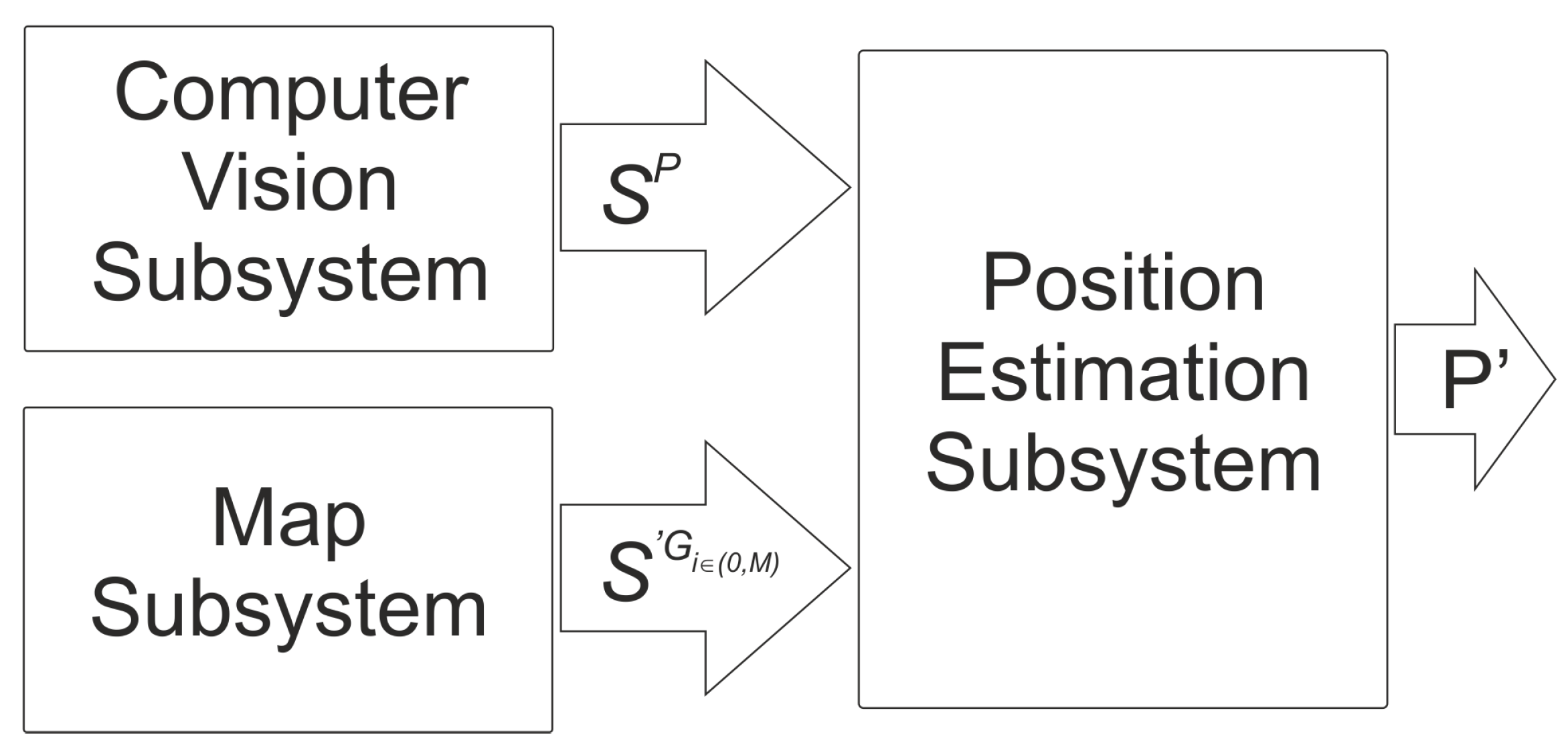
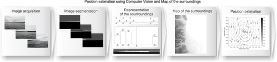
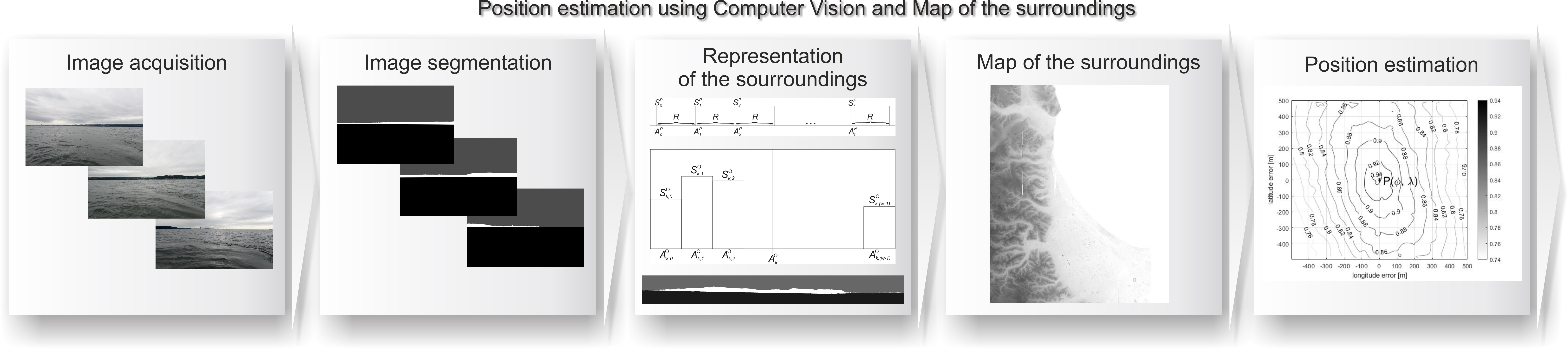
The solution outlined in this paper represents an innovative approach to determining the X,Y coordinates of an AUV through the integration of advanced computer vision and artificial intelligence methods. This advanced methodology is mainly applied in AUV navigating areas without radio navigation signals. During a temporary surface, the system captures images of the environment using a camera mounted on the vehicle. The semantic segmentation is then performed using a trained neural network, the purpose of which is to obtain information about the height of the land in a given bearing. The resulting output provides a comprehensive representation of the vehicle’s environment, facilitating comparative analysis with a corresponding map-derived representation. The complex architecture of the proposed system is illustrated by the components shown in
Figure 1:
Where:
—the representation of the surroundings of the vehicle at point P
P—the point where the vehicle is actually located
—map representations of the points ,
M—the set of random points
—point on the map where the map representation is created
—estimated AUV position.
3.1. Computer Vision Subsystem
The task of the subsystem is to determine the visual representation of the vehicle surrounding
in point
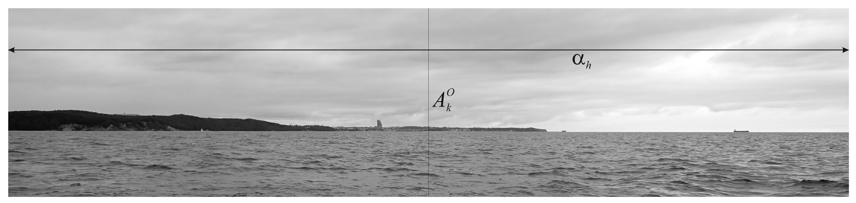
P, where the actual location of the vehicle is. A camera mounted on the vehicle is used for this purpose. The vehicle or camera is rotated
to provide full coverage of the surroundings. Actual camera angle information
is read from on-board systems and appended to each
kth image,
. Knowing this parameter and the horizontal angle of view
, the bearing (angle) can be determined for each image pixel column (
Figure 2).
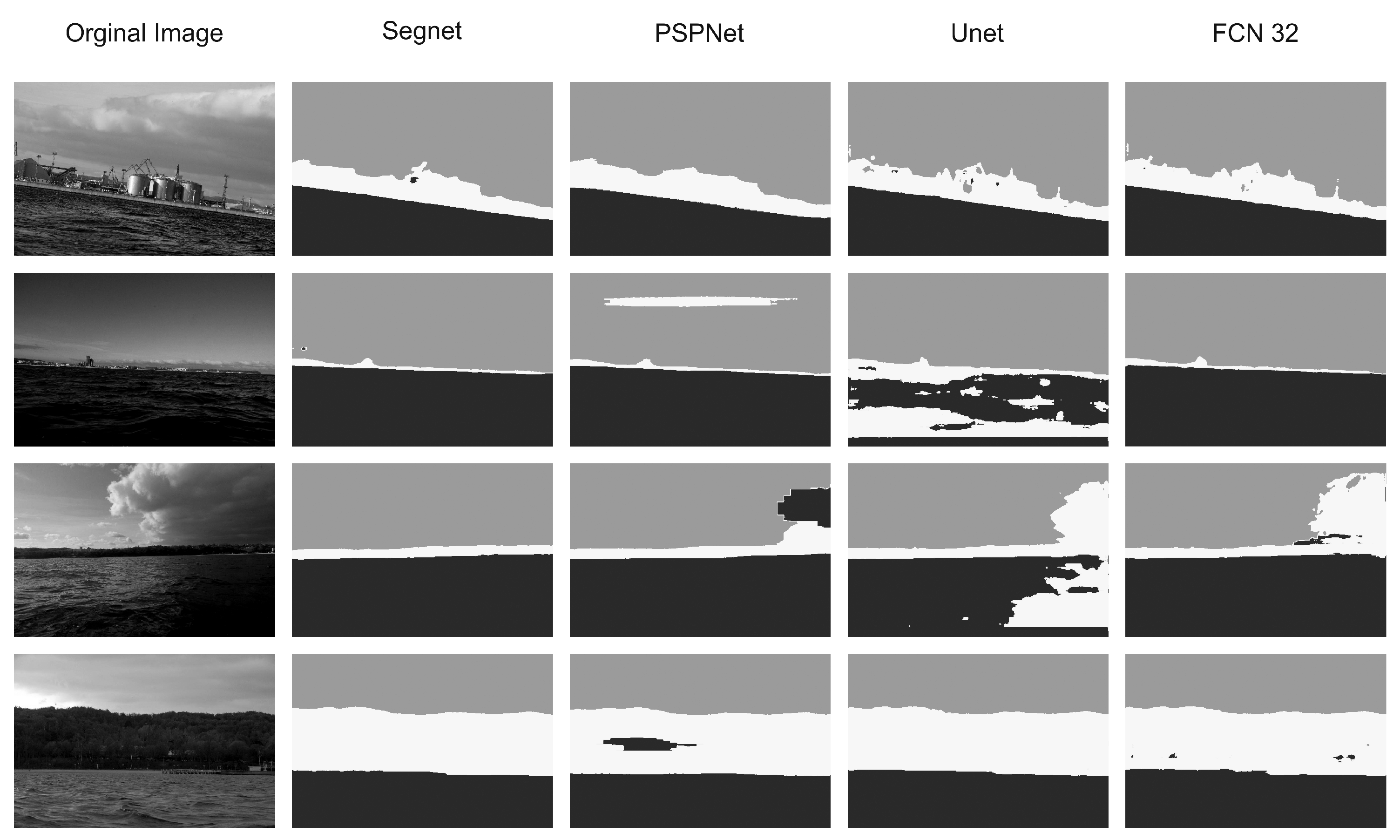
The recorded images are then segmented to determine where the land is located. This is done using a trained convolutional neural network (
Figure 3).
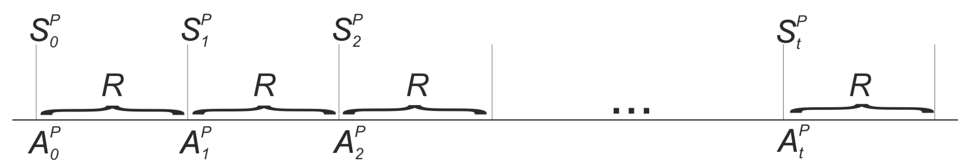
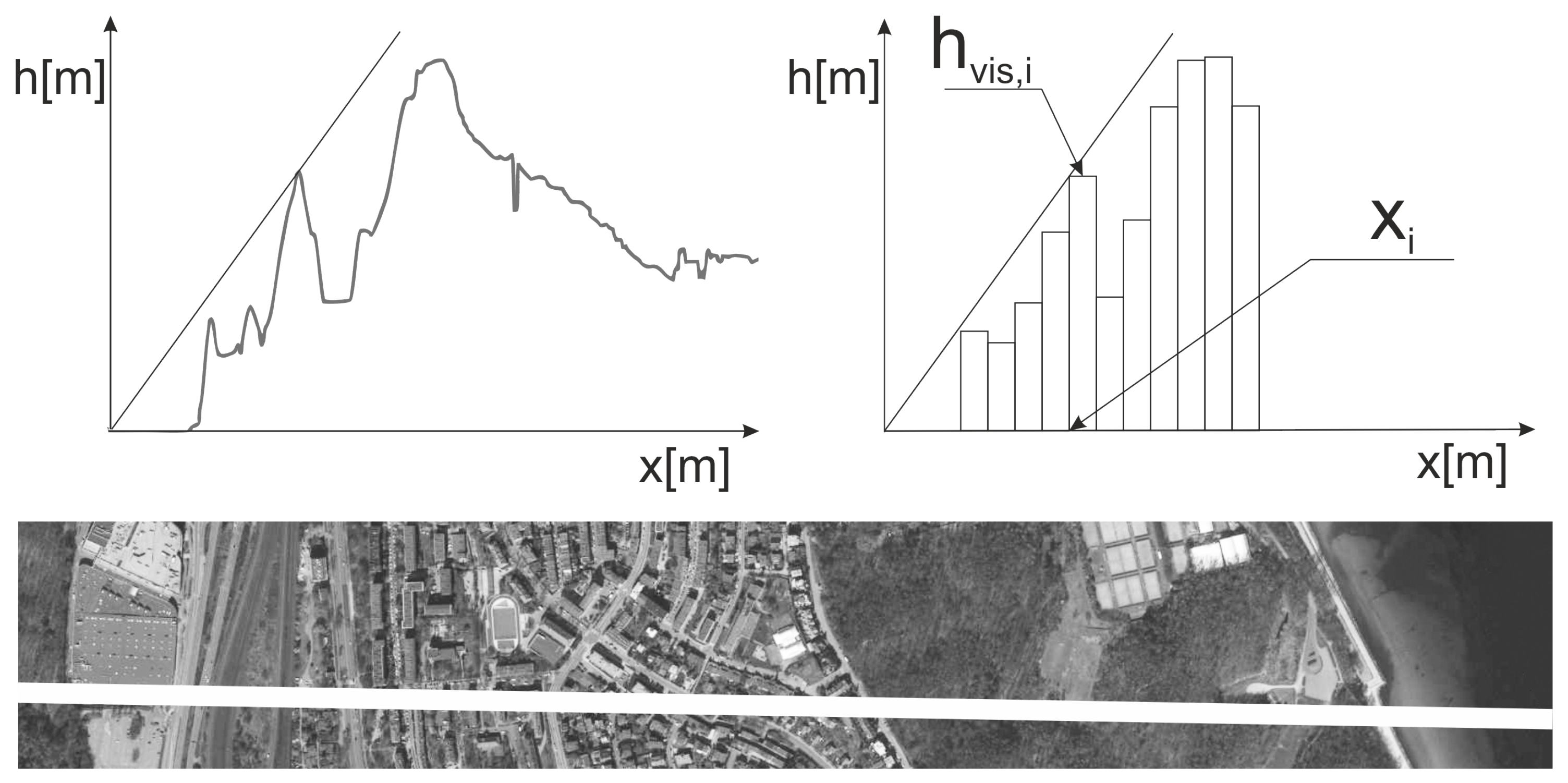
The information from all segmented
N images is then used to create a representation of the vehicle’s surroundings
. Formally, the representation
(
Figure 4) is the height of the land as seen from the point
P, where
is the height of land in the direction
,
,
, and
R is the resolution of
.
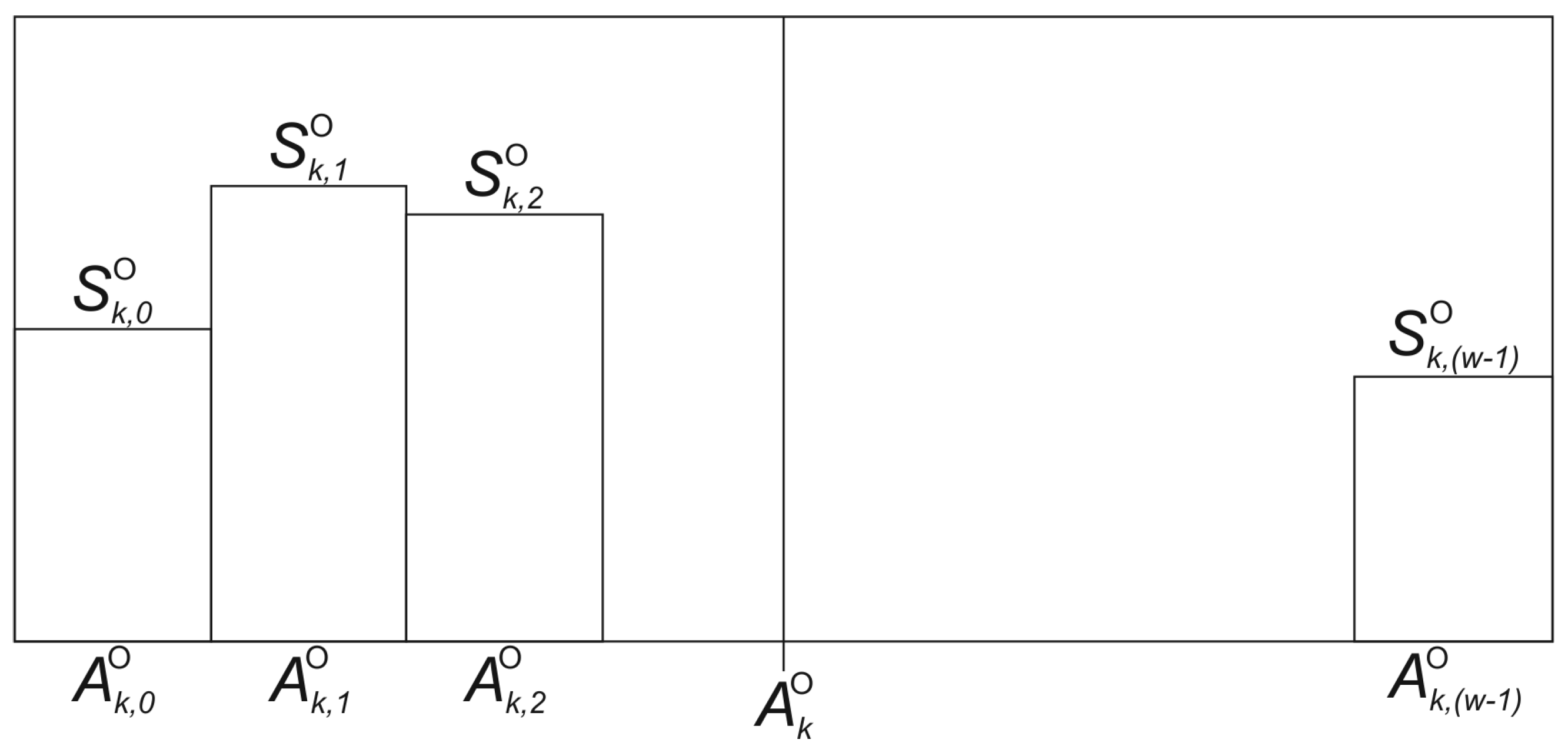
is determined from the
N images captured by the camera, of which the
kth image is represented by (
Figure 5):
where:
—is height of land in kth image and ith image column;
—is azimuth (angle) for kth image;
—is azimuth (angle) for kth image and ith image column;
w—determines the width of the image.
Finally,
is calculated as follows:
where:
—is the image that was selected to calculate
—is the column of image, which was selected to calculate .
3.2. Map Subsystem
The primary objective of the subsystem is to generate a map representation
corresponding to any given point
in the area covered by the terrain model. This representation is formulated by integrating a stored topographic map, a digital terrain model, or, in particular, a digital surface model. Of these options, the digital surface model emerges as the most accurate representation of the terrain, as it not only encapsulates the topographical features, but also incorporates elevation information relating to objects on the ground, such as trees and buildings, thereby increasing the overall accuracy of the representation. The construction process
requires the application of appropriate transformations, taking into account the Earth’s curvature and the objects’ mutual occlusion, as shown in
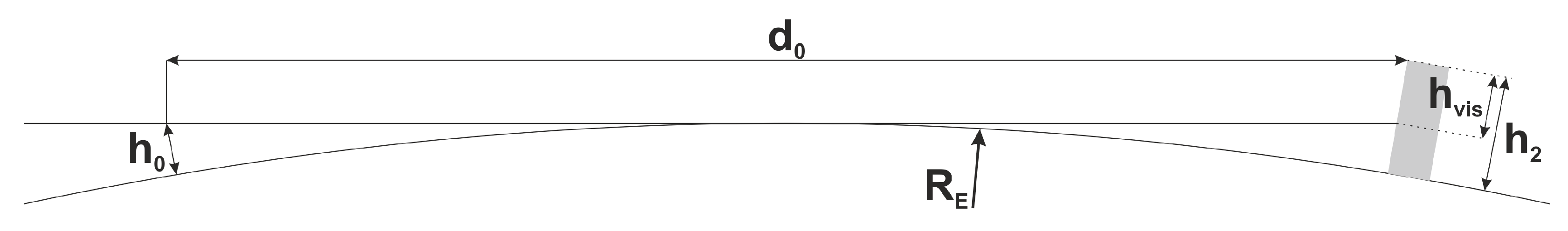
Figure 6. This complex process ensures a faithful representation of the terrain that is consistent with the topography of the real world. A critical consideration in this endeavor is the phenomenon of mutual occlusion, where objects occlude each other as the observer moves away from them. The size of the visible portion (
) of an object is mainly a function of the elevation of the camera and the distance from the object, as described by Equation (
3). This mathematical relationship emphasizes the dynamic nature of the visible part of an object as a function of both camera placement and spatial proximity. The systematic consideration of these factors is essential for the accurate and comprehensive generation of the map representation
, which reflects the complex interplay between terrain features and observation parameters.
Figure 6.
Height of an object beyond the horizon [
49].
Figure 6.
Height of an object beyond the horizon [
49].
where:
—height of observer (camera)
—height of an object visible above horizon
—height of an object
—distance from the observer to object
—radius of earth.
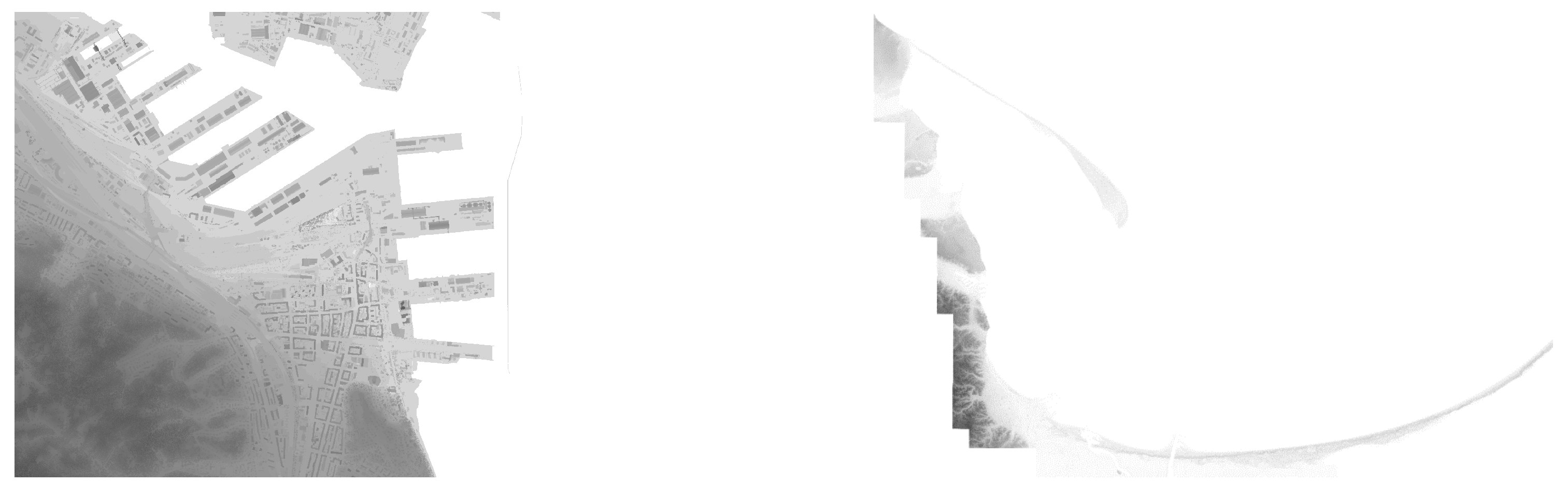
In addition, there are cases where the apparent height of an object in the foreground is less than that of a more distant object, but the former still blocks the view of anything behind it. This scenario is particularly relevant in the context of map creation, where the goal is to capture information about objects that occupy the largest number of pixels in the image, prioritizing visibility over physical height.
Figure 7 presents a visibility analysis carried out along a specified line of approximately 4 km, accompanied by its corresponding cross section or elevation profile. This analytical display illustrates the nuanced interplay between foreground and background objects and highlights the critical nature of prioritizing pixel coverage in the display process. The intricacies of visibility, as delineated in the cross section, underscore the need for a sophisticated approach to map representation that goes beyond mere physical height considerations to ensure a more comprehensive and contextually relevant representation of the observed terrain.
Formally, a map representation for point
looks as follows:
where:
—a numbered sequence of pixels in direction from point
—distance from point to the ith pixel.
3.3. Position Estimation Subsystem
The task of the subsystem is to determine the position estimated at point
P. This is done by comparing the
representation with the
map representations for the set
M of random points
located in a circle with radius
r and center at point
Q, which is the estimated position of the submersible vehicle determined by the dead reckoning navigation system. The position of point
P corresponds to the position of point
, whose representation
is more similar to the representation of
with respect to the selected measure of similarity
T. Formally, the estimated position
for the point
P is defined as follows:
where:
T is a measure of the similarity of representations and .
5. Experimental Results
In order to verify the effectiveness of the proposed algorithm, the errors (max, min, and average) in the calculation of the estimated position
for each point
P were applied. The errors are given in
Table 2.
As it turned out, errors in the estimation of the position
P for Equation (
9) were 102.40 m (max), 8.93 m (min), and 64.60 m (avg). For Equation (
8), the results were significantly worse and were 189.25 m (max), 10.43 m (min), and 91.6 m (avg). Pearson’s correlation, as a measure of the linear relationship between variables, showed greater sensitivity to underlying patterns. This is particularly important for data where the relationships between variables are not strictly linear and may show non-linear trends. Unlike Euclidean distance, which is sensitive to the size and scale of the variables, Pearson’s correlation takes into account relative differences, providing a more robust measure of similarity. The prevalence of Pearson correlation in our experiments suggests that it is more appropriate for our dataset.
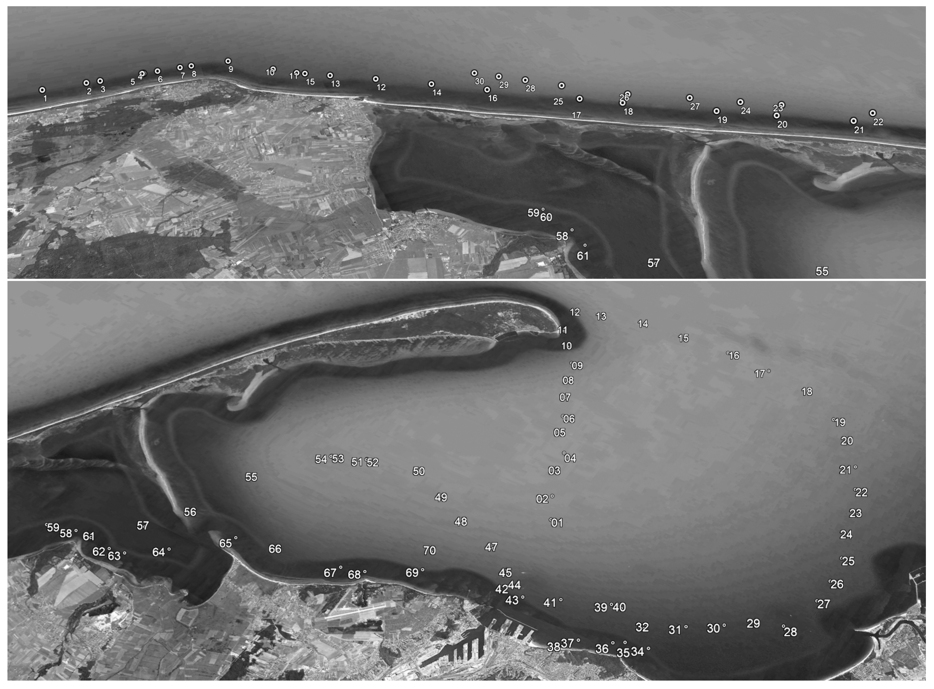
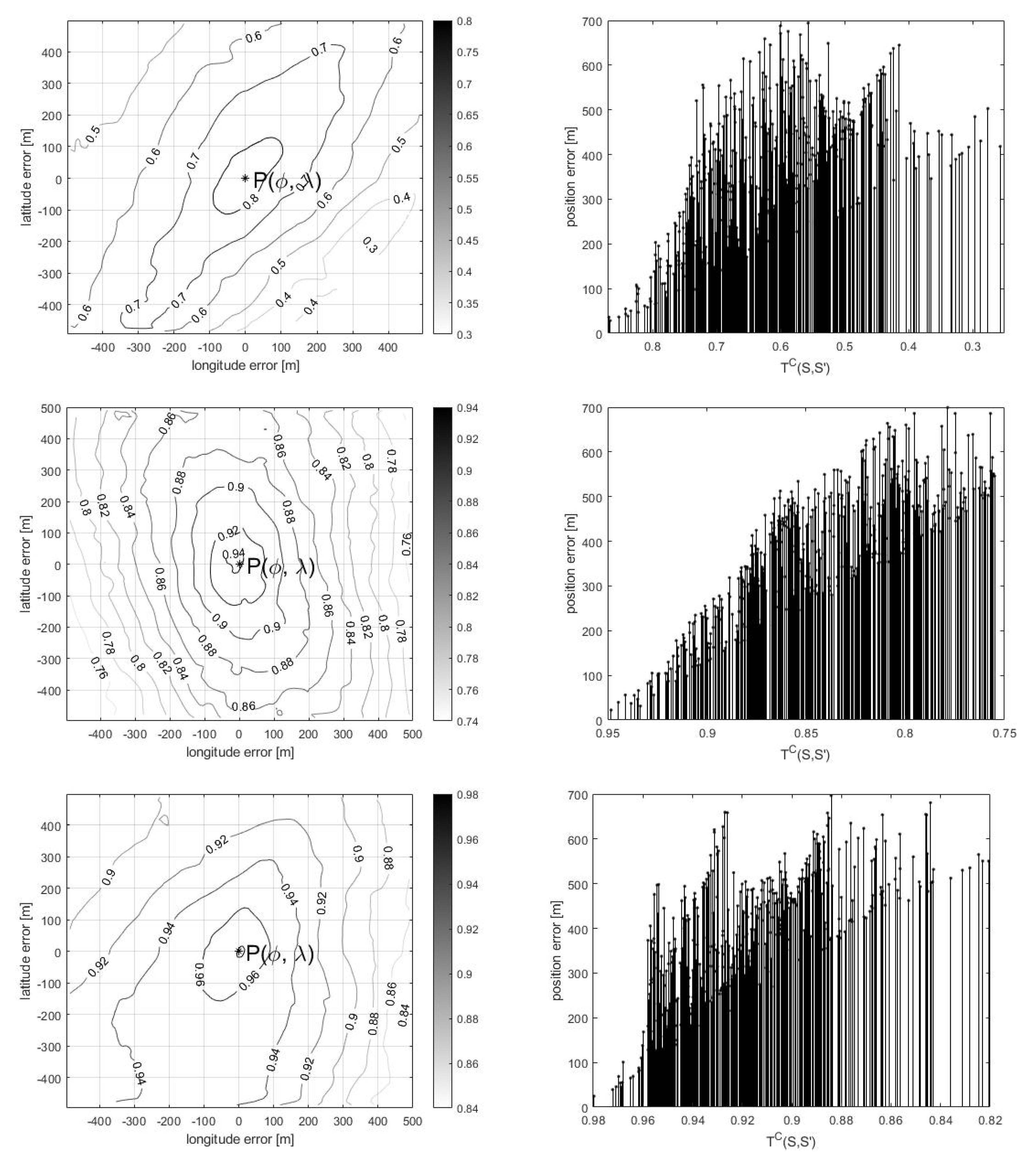
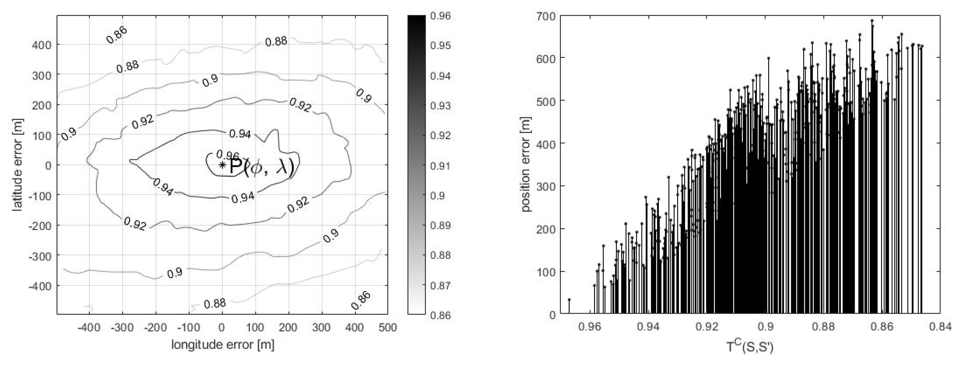
After the analysis of the spatial distribution of the points
, it turned out that the points with the highest similarity measure
were generally located in the closest neighborhood to the point
P. The distribution of the correlation coefficient for four sample points
P is shown in
Figure 12 (left column). The authors thus decided to estimate
based on the five
points with the highest
according to the following equation:
where:
L—a set of points with the highest value of .
Figure 12.
Distribution (left—spatial, right—quantitative) of the correlation coefficient for four sample points P.
Figure 12.
Distribution (left—spatial, right—quantitative) of the correlation coefficient for four sample points P.
As it turned out, this procedure resulted in a significant reduction in the estimation error, as shown in
Table 3.
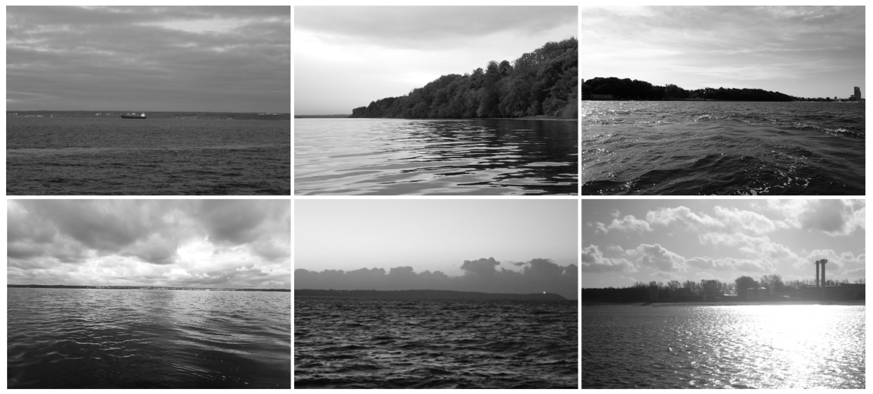
During the registration of the images, there were situations where the sea conditions (waves) or the appearance of surface vessels in the field of view prevented the correct generation of the representation
. Therefore, the authors decided to verify the effectiveness of the incomplete environment representation algorithm
. To this end, 10%, 30%, or 50% (in reality, it is very unlikely for the disruptions to exceed 30%) of items, ranging from the
nth to the
mth, were removed from
. The resulting representation
after the removal procedure is given by Equation (
11). The verification of the algorithm for incomplete representation
was carried out for 20 random points
P, and the results are presented in
Table 4.
where:
.
Table 4.
Comparing representations of incomplete surroundings.
Table 4.
Comparing representations of incomplete surroundings.
| Removed Part | n | Min [m] | Max [m] | Average [m] |
|---|
| 10% | 180 | 5.21 | 54.19 | 40.87 |
| 10% | 720 | 7.87 | 74.02 | 29.08 |
| 10% | 1800 | 4.17 | 62.94 | 47.78 |
| 30% | 180 | 8.03 | 81.09 | 46.26 |
| 30% | 720 | 14.01 | 101.29 | 69.01 |
| 30% | 1800 | 10.65 | 57.94 | 36.28 |
| 50% | 180 | 42.39 | 179.03 | 130.97 |
| 50% | 720 | 38.67 | 237.14 | 158.30 |
| 50% | 1800 | 49.49 | 213.59 | 143.00 |
The obtained results show that incomplete display around the vehicle does not make it impossible to estimate vehicle position. For disruptions equal to 10% and 30% of original
, the highest errors amounted to 47.78 m/69.01 m (average), 74.02 m/101.29 m (max), and 7.87 m/8.03 m (min), which is an even better result than for the undisturbed representation
. However, it should be noted that the results given in
Table 3 are calculated for only 20 measurement points compared to the previous case in which all 100 points were considered. The noticeable deterioration of the results is only visible for 50% of the disturbances. In this case, the highest errors amounted to 158.30 m (average), 237.14 m (max), and 49.49 m (min).
6. Future Research
The exploration of alternative terrain models is a promising avenue for further research. While DSM provides high accuracy in object elevation information, they are limited to specific geographic regions. In cases where DSM data are not available, alternative models as topographic maps or satellite imagery could be used. However, this will require adaptations to the existing algorithm to enable it to integrate and utilize different map information from different sources.
A second area of research is the development of an algorithm tailored to regions with recognizable landmarks in the vicinity of the vehicle. For this purpose, a terrestrial navigation approach can be used by training neural networks to classify objects such as forests, beaches, lighthouses, buoys, etc., and then using an algorithm to locate these objects on a map. This approach is promising in environments where identifiable landmarks can serve as navigational reference points.
The third area of interest revolves around exploring the size of objects in the image. By identifying objects of known size and estimating their distance based on the disparity between their actual size and their size in pixels, a methodology for distance estimation can be established. Integrating this distance information with object classification data further paves the way for an effective terrestrial navigation approach.
A fourth and equally important area for future research is the development of algorithms capable of detecting image clutter such as waves, vessels, and other potential sources of interference. The identification and mitigation of such clutter is critical to ensuring the accuracy of vehicle position calculations, particularly in challenging marine environments where external factors can impede accurate navigation.


