1. Introduction
With the implementation of increasingly growing earth observation programs, RS images and street-view images have been explosively booming, and we have entered an age of big RS data [
1,
2,
3]. Cross-view geo-localization aims to determine the location of a query street-view image by retrieving the most similar image in a GPS-tagged RS image dataset. Cross-view geo-localization plays an essential role in noisy GPS correction, event detection, accurate delivery, autonomous vehicles, and so on [
4].
Cross-view geo-localization can be regarded as an image retrieval task [
5,
6,
7,
8,
9,
10,
11,
12]. As shown in
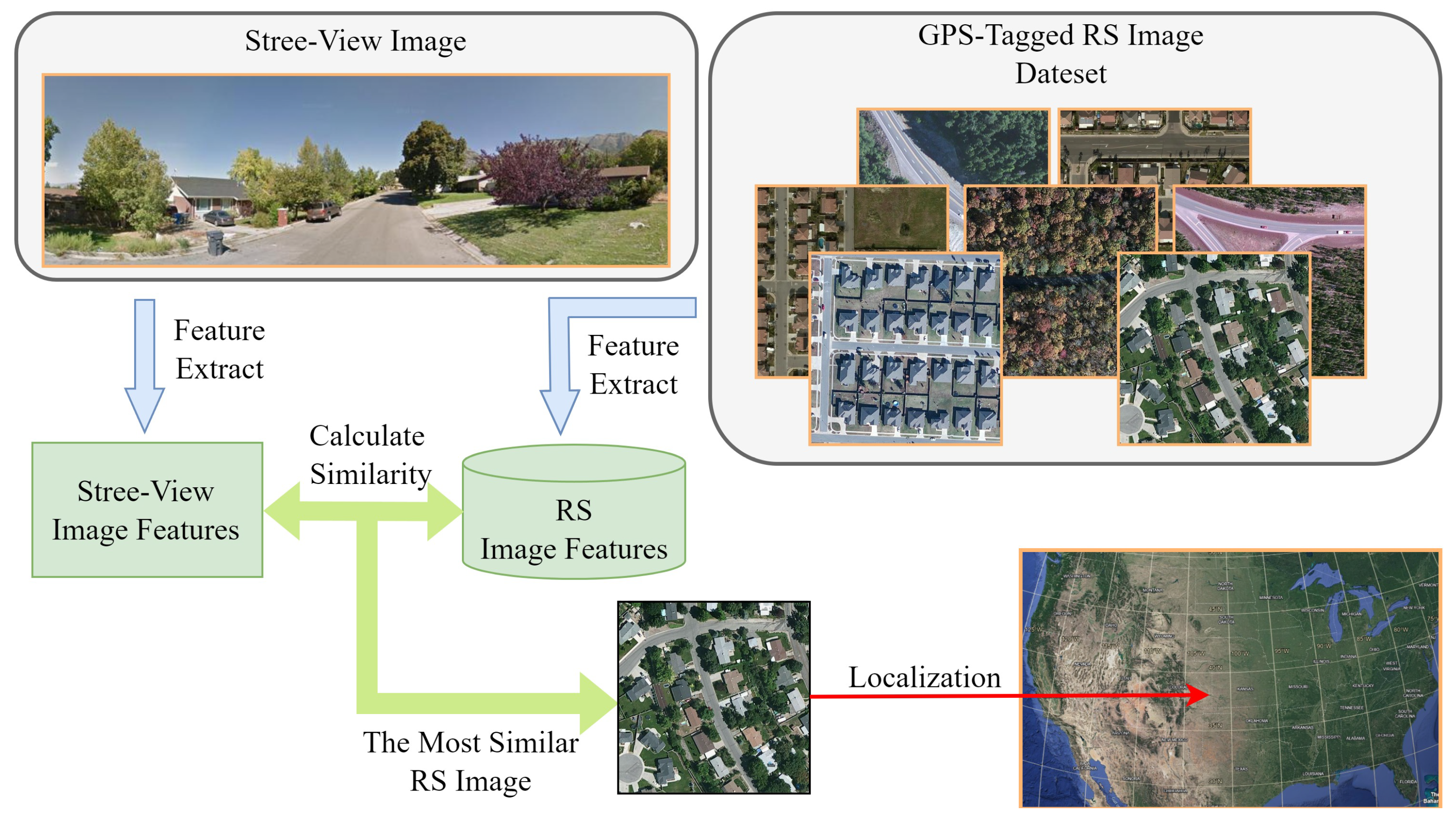
Figure 1, firstly, features are extracted from a queried street-view image and RS images. Subsequently, the similarity between the features of the street-view images and RS images is computed, and the RS image with the highest similarity is selected. Therefore, we can locate the street-view image using the GPS coordinates from the selected RS image. Cross-view geo-localization faces major challenges arising from significant domain differences between street-view images and RS images. The domain gap primarily involves two aspects. On the one hand, there are considerable viewpoint differences between street-view images and RS images, as street-view images are centered around the shooting location, while RS images are orthorectified. On the other hand, the appearances of street-view images and RS images may vary significantly due to the possibility of being captured at different times and with different cameras, seasons, weather, and lighting.
Recently, deep learning-based methods [
8,
9,
10,
13,
14,
15,
16] have been dominant in cross-view geo-localization. They generally train a dual-channel Siamese network framework to extract features from street-view images and RS images, respectively. Therefore, the component for feature extraction plays a vital role in deep learning-based cross-view geo-localization models.
A CNN (convolutional neural network) is the most commonly used feature extraction component for cross-view geo-localization, whereas CNN-based models face challenges in establishing the corresponding relationship between the street-view images and RS ones, because the two types of images from different domains have significant viewpoint differences.
To address the viewpoint differences issue between street-view images and RS images, a defined polar transform [
12] and GANs (Generative Adversarial Networks) [
17] are leveraged to make the transformed RS images look like the corresponding street-view images [
18,
19,
20]. The polar transform proposed by Shi et al. [
12] is a mathematic transform and requires determining the orientation relationship between street-view images and RS images. Therefore, the polar transform may fail when the two types of images have different lighting conditions or the street-view images are not spatially aligned at the center of the RS images [
6]. The GAN-based domain adaptation models for cross-view geo-localization involve significant computational costs and may suffer from model collapse.
The vision-transformer (ViT) [
21] has powerful global modeling capability and a self-attention mechanism. The ViT-based models [
22,
23,
24] for cross-view geo-localization can effectively model the potential dependency between the street-view images and the corresponding RS images, but they only generate one single feature map and do not consider extracting multi-scale features, potentially leading to information loss.
In summary, the current models mainly face challenges in addressing viewpoint differences and information loss caused by downsampling. To tackle these issues, this paper proposes a swin-transformer-based model.
Recently, swin-transformer [
25] has demonstrated competitive performance across various vision tasks. Using swin-transformer for geo-localization has the following advantages. First, the use of position encoding technology in swin-transformer facilitates our model in learning the geometric relationships between street-view images and RS images, allowing it to address the impact of differences in their viewpoint. Secondly, swin-transformer employs multiple stages for downsampling and feature extraction. This implies that swin-transformer has the potential to extract features at different scales and pay attention to more diverse features. Building upon this, we modified the swin-transformer model to extract features at different scales from different stages, resulting in multi-scale features. We believe that the extracted multi-scale features that encompass more diverse information can facilitate the accuracy of cross-view geo-localization.
Moreover, in order to enhance the robustness of extracting and aligning meaningful multi-scale features between street-view images and RS images, we introduce contrastive learning [
26] to the proposed model. Contrastive learning is a self-supervised learning method that aims to learn meaningful representations by maximizing the similarity of similar samples and minimizing the similarity of dissimilar samples, which is advantageous to extract more meaningful and robust features in supervised learning tasks [
27].
In this paper, we propose an end-to-end multi-scale feature-extracting and -matching neural network (GeoViewMatch) using swin-transformer and contrastive learning for cross-view geo-localization. The positional encoding technique facilitates the GeoViewMatch in learning the geometric positional relationships between street-view images and RS images [
23]. This contributes to resolving the issue of viewpoint differences between street-view images and RS images. GeoViewMatch extracts features at different scales, enabling it to focus on more diverse information. Furthermore, GeoViewMatch incorporates contrastive learning to enhance the robustness of extracting and aligning features.
Our contributions can be summarized as follows:
A novel and lightweight end-to-end model is proposed to extract comprehensive multi-scale features from street-view images and RS images for cross-view geo-localization. In addition, it can be easily applied to other cross-view information retrieval tasks, such as UAV images and satellite images.
A contrastive learning component is designed to lift the robustness of extracting and aligning meaningful multi-scale features between street-view images and RS images, which can further facilitate the performance of the proposed model. To the best of our knowledge, this is the first work to consider the potential intentions of contrastive learning in the cross-view geo-localization task.
We demonstrate the effectiveness and advantages of the proposed method through comprehensive experiments. The proposed model outperforms the state-of-the-art results on two common benchmarks with less computation costs, parameter counts, and inference time than other end-to-end methods.
The remaining part of this paper is organized as follows. The related work is shown in
Section 2. In
Section 3, we show the details of the GeoViewMatch architecture. In
Section 4, we provide the experiment materials and results. The discussion and conclusion are mentioned in
Section 5 and
Section 6.
2. Related Work
2.1. Cross-View Geo-Localization
Early geo-localization can be divided into two categories: methods based on digital models [
28,
29,
30] and methods involving manually designed features [
31]. The methods based on digital models involve constructing three-dimensional digital models of the terrain or buildings for geo-localization. However, this approach requires constructing high-precision three-dimensional digital models, making it challenging to generalize to large-scale geo-localization. The manual feature extraction methods based on self-similarity and color histograms face challenges in achieving satisfactory results in retrieval accuracy.
With the advancement of deep learning methods, several approaches based on deep learning have also been introduced. Workman et al. [
32] first employ a CNN to address the problem of cross-view geo-localization and construct one of the most popular datasets in this field, called CVUSA. To bridge the domain gap between street-view images and RS images, Wang et al. [
5], based on the behavioral characteristics of humans when comparing images, divide the deep features extracted by the network into centrally pyramid-shaped blocks, significantly improving the retrieval accuracy. Nevertheless, the pyramid-shaped blocks may not necessarily delineate valuable regions. Shi et al. [
12] design a polar transform algorithm so that the transformed RS images have spatial layouts similar to street-view images. Similarly, to address the domain gap, Regmi et al. [
33] use GANs to generate more realistic street-view images from RS images. On this basis, Toker et al. [
20] utilize polar-transformed images to generate street-view images. However, they rely highly on the geometric correspondence of street-view images and RS images [
23]. Shi et al. [
34] employ optimal transport theory for features transport, aligning street-view image features with RS image features. Weyand et al. [
7] divide the world into a grid network, creatively treating cross-view geo-localization as a classification problem. The output of the method is a probability distribution worldwide. Nonetheless, obtaining high-precision coordinates requires a finer grid network, which would make the output layer significantly large. Yang et al. [
35] is the first model to use the VIT for cross-view geo-localization. Zhu et al. [
23] propose a pure transformer-based method using a two-stage pipeline. These indicate the potential of the transformer in the field of cross-view geo-localization. The ViT adopts a relatively aggressive downsampling strategy and generates a single low-resolution feature map, making it challenging for the model to extract multi-scale features and lose some fine diverse features.
2.2. Swin-Transformer and Its Application
CNN-based methods encounter challenges in dealing with viewpoint differences in cross-view geo-localization. Due to the relatively aggressive downsampling strategy, the ViT may lose some diverse features. Swin-transformer [
25] has shown competitive performance in various computer vision tasks, including image classification [
36], object detection [
37], road extraction [
38], and image restoration [
39]. Compared to the ViT and the CNN, swin-transformer has the following advantages: (1) Shifted Window-based Self-Attention [
40]: This mechanism divides the image into fixed-size non-overlapping windows, with each window utilizing a self-attention mechanism internally, reducing computational complexity. (2) Multi-level Attention: This includes both Local Tokens and Global Tokens. This multi-level attention mechanism enables the model to better extract features at different levels and scales. (3) Local and Global Information Fusion: Swin-transformer integrates local and global attention to better capture both local and global information in images, enhancing the understanding and representation of image structures. (4) Multiple Stages: Swin-transformer consists of multiple stages that progressively downsample the input and extract features at different scales. Utilizing the aforementioned advantages, swin-transformer can extract multi-scale features with more diverse features. Additionally, the position encoding in swin-transformer contributes to the model’s capacity for learning intricate geometric relationships, effectively mitigating challenges associated with variations in viewpoint.
2.3. Contrastive Learning
Contrastive learning has been widely applied in computer vision, including tasks such as image classification [
27,
41,
42] and object detection [
43]. Methods such as SimCLR [
27] and MoCo [
42] have achieved results surpassing traditional supervised learning on large-scale datasets. MoCo introduces momentum contrast, being the first unsupervised model to surpass supervised models in many mainstream computer vision domains. SimCL achieves performance improvement by incorporating a simple projection head. MoCo3 [
44] and Dino [
43] address the issue of the instability of training the ViT as a backbone and successfully introduce the transformer into contrastive learning. Contrastive learning typically employs a variety of methods for data augmentation. Data augmentation techniques include image manipulation, rotation, translation, shearing, flipping, cropping, resizing, kernel filters, etc. Applying contrastive learning to our model and selecting appropriate data augmentation techniques can enhance the model’s ability to cope with changes in lighting, time, and other variations, thereby improving the robustness and alignment of feature extraction in the model.
3. Methods
We first introduce our pipeline in
Section 3.1. In
Section 3.2, we describe the Swin-Geo module used in our model and how it extracts multi-scale features. We introduce how we incorporate contrastive learning into our model in
Section 3.3. Finally, we introduce the design of the loss function in
Section 3.4.
3.1. Overview of Method
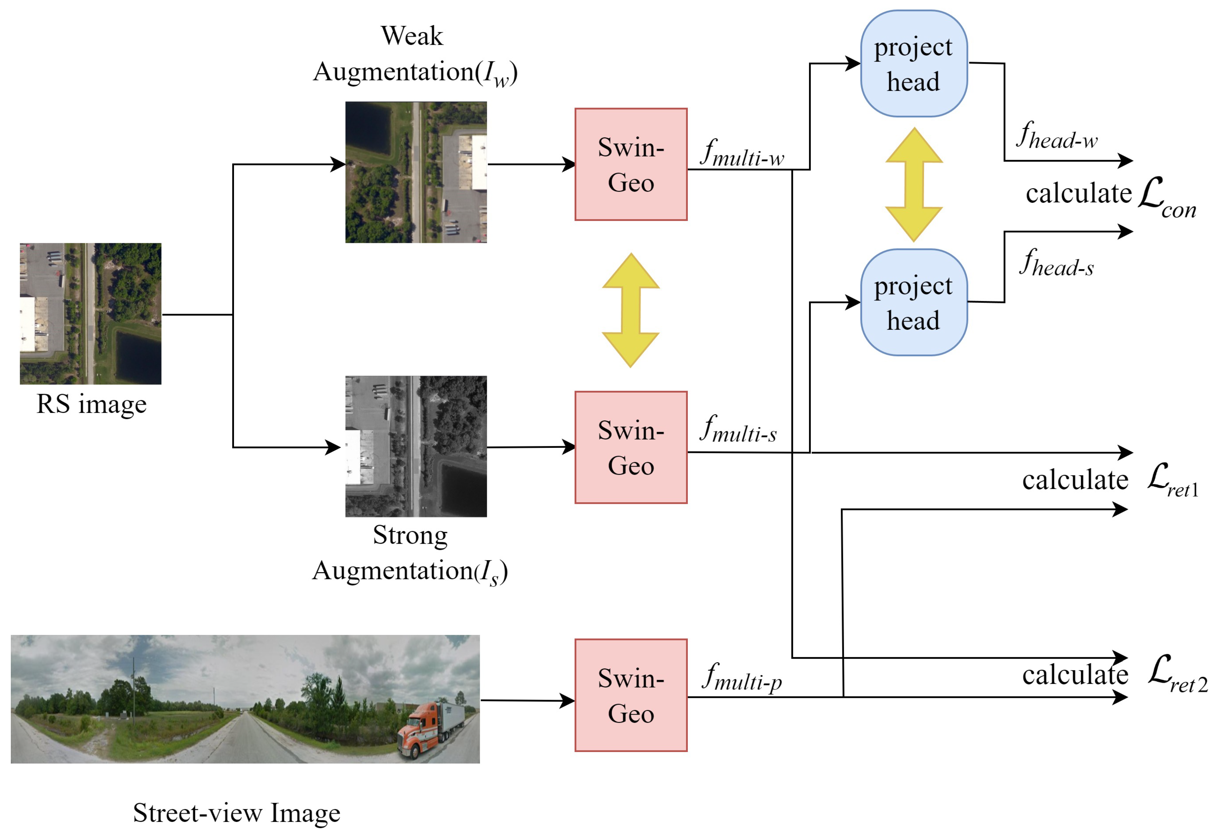
The overview of our method, GeoViewMatch, is shown in
Figure 2. We treat cross-view geo-localization as an image retrieval task. GeoViewMatch also adopts a Siamese network framework, but what sets it apart from previous models is the simultaneous incorporation of a contrastive learning framework and using the Swin-Geo module to generate feature maps at different scales and to extract multi-scale features.
A project head consists of two fully connected layers. Specifically, GeoViewMatch utilizes pairs of RS images and street-view images as inputs. For the RS images, GeoViewMatch applies both strong and weak augmentations to obtain enhanced images and . These images and are inputted into two shared-weights Swin-Geo modules, resulting in multi-scale features and features . The street-view images are also processed through a Swin-Geo module. Unlike RS images, we do not apply strong and weak augmentations to street-view images.
3.2. Swin-Geo
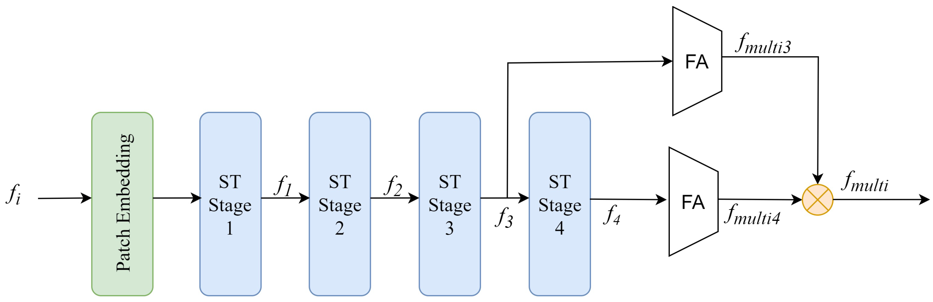
The structure of Swin-Geo is shown in
Figure 3. Swin-Geo utilizes swin-transformer as its backbone, comprising four stages, each containing a downsampling module to generate features at different scales. A feature
is processed through Swin-Geo, and the four stages of Swin-Geo generate features
,
,
, and
, where the
and
denote the output channels and spatial dimensions of ST Stage-4. The traditional swin-transformer utilizes a simple average pooling layer and a linear layer for feature aggregation, leading to information loss and proving unsuitable for geo-localization tasks. Inspired by [
12,
20], we introduce a module for feature aggregation. The features
and
pass through the feature aggregation module and then the output features
and
are concatenated to obtain the multi-scale features
.
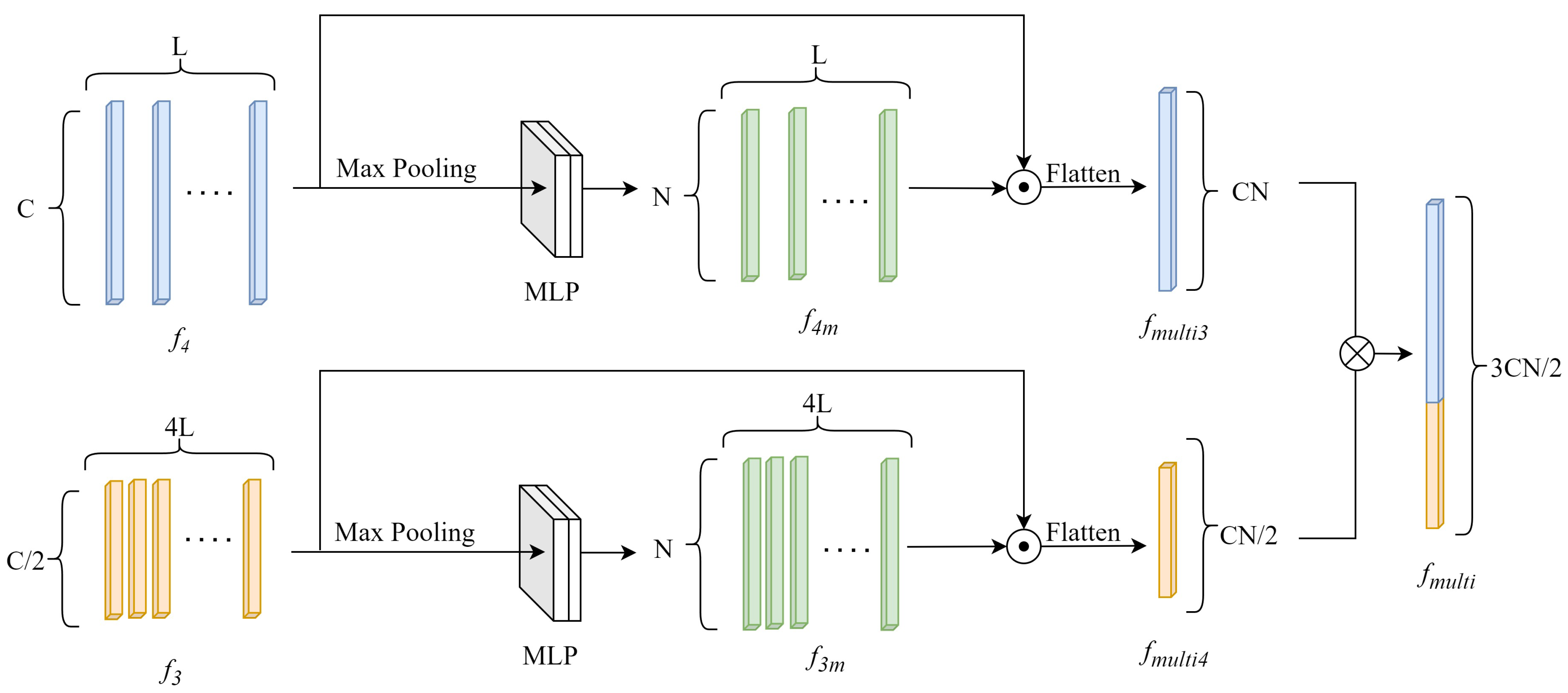
Multi-scale Features and Feature Aggregation Module: Different ST Stages produce features at different scales. GeoViewMatch selects features from ST Stage-3 and ST Stage-4 to construct multi-scale features. Inspired by the works [
12,
20], a module is employed to aggregate these two features, resulting in multi-scale features. As shown in
Figure 4, the input features
and
undergo max pooling followed by MLP layers, resulting in features
and
.
is subjected to a Frobenius inner product with
, while
undergoes the same operation with
. This yields
and
. The final multi-scale features
are obtained by concatenating
and
.
3.3. Contrastive Learning in GeoViewMatch
To bolster the robustness of extracting and aligning meaningful multi-scale features, we introduced contrastive learning in GeoViewMatch. While traditional contrastive learning relies on large datasets for pre-training, GeoViewMatch skips the pre-training step. Instead, it directly introduces contrastive learning during training, utilizing soft-margin triplet loss [
9] in place of the traditional NEC-loss [
44] as the contrastive loss. For an inputted image, after undergoing strong and weak augmentations, GeoViewMatch ultimately outputs two multi-scale features. These features pass through a shared-weights project head, and the contrastive loss is calculated. This loss aims to maximize the similarity between the matched strongly and weakly augmented images and to minimize the similarity of the mismatched images, thereby enhancing the model’s information extraction capabilities.
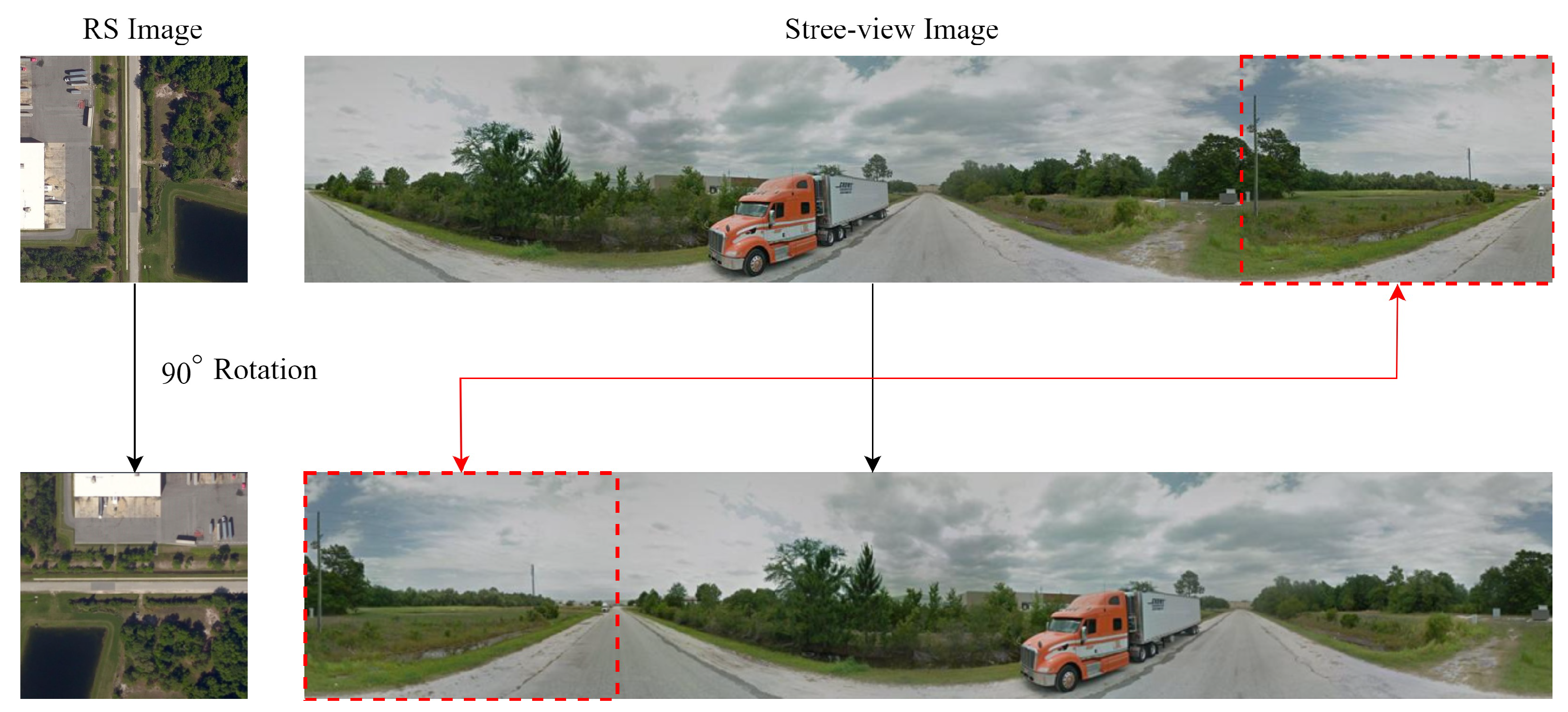
For RS images, we choose random color jitter, random gray, and Gaussian blur as strong augmentation. Weak augmentation generally consists of geometric transformations, altering the geometric relationships of objects within the image. We chose random rotation as weak augmentation, with rotation angles limited to clockwise 90, 180, and 270 degrees. It is noteworthy that the orientations of street-view images and RS images need to be aligned. To preserve this alignment, street-view images can be transformed by moving one side of the image to the other, and the proportion and direction of the movement corresponding to the rotation angle of the RS image.
Figure 5 is an example of a clockwise rotation of 90 degrees. Unlike RS images, we do not apply strong and weak augmentations to street-view images. We believe RS images are more susceptible to changes in cloud cover, shadows, lighting, and season, emphasizing the importance of extracting robust features from RS images.
3.4. Loss Function
The loss of GeoViewMatch is composed of retrieval loss (
and
) and contrastive loss (
), and it is trained using the soft-margin triple loss [
9]:
where
and
represent the squared
distance of the positive and negative pairs, and
denotes the weight of the soft-margin triplet loss. In the retrieval loss, the positive pairs are the matched street-view images and RS images, while the negative pairs are the mismatched street-view images and RS images.
In the contrastive loss, strongly augmented images and weakly augmented images from the same source images are considered positive pairs, while those from different images are treated as negative pairs. We apply
normalization to all the features. The total loss consists of three components:
where the
,
, and
are the weights of
,
, and
.
4. Experiment
4.1. Datasets
We conduct comprehensive experiments on two widely used datasets, CVUSA [
32] and CVACT [
10].
The CVUSA dataset is collected in the United States and comprises over one million street-view and RS image pairs, encompassing a mixture of commercial, residential, suburban, and rural areas. The initial proposal of the CVUSA dateset is aimed at large-scale localization across the United States. Following the previous works [
12,
20,
23], we use a subset of the CVUSA dataset. The subset was created by Zhai et al. [
45]. In the process of creating this dataset, they utilized the external parameters of the camera to align the image pairs by warping street-view images. This dataset comprises 44,416 pairs of street-view images and RS images. We utilize 35,532 of them for training and the remaining 8884 for validation. The size of the street-view images and RS images are
and
. Additionally, there are street-view semantic segmentation labels in the CVUSA dataset, but we do not use them.
The CVACT dataset is collected in Australia. Compared with the CVUSA dataset, the CVACT dataset includes more urban and suburban images with a higher resolution, but the ground coverage includes cultivated land. To maintain consistency, the CVACT dataset has the same size train set and validation set as the CVUSA dataset. The size of the street-view images and RS images are and . The ground solution for the RS images is 0.12 m per pixel.
4.2. Evaluation Metric
Following the previous works [
12,
20,
23], we use top-k recall accuracy (
) as the standard evaluation protocol. Our algorithm can output a set of plausible matches based on the cosine similarity for each street-view image and RS image. The
value is defined as the position within the rankings of the ground-truth RS images that are correctly identified among the top-k matches for a given street-view image. As the primary objective of cross-view geo-localization is to minimize the localization error, quantified in meters, following [
6,
23], we calculate the distance between the retrieved images and the street-view images. If this distance is below a predefined threshold, it is considered a successful retrieval.
4.3. Implementation Details
Our algorithm is implemented using PyTorch [
46]. For the CVUSA dataset, the street-view images and RS images are resized to
and
. For the CVACT dataset, the RS images are also resized to
, but the street-view images are first cropped to
and then resized to
.
For the model, we employ swin-transformerV2-tiny as the backbone. The patch size is
, and the out features dimension is 768. Swin-transformer contains four stages, and each stage consists of 2, 2, 6, and 2 swin-transformer blocks. Each stage’s multi-head attention module includes 3, 6, 12, and 24 heads, respectively. Moreover, we discarded the average pooling and classification head in swin-transformer, opting instead for a feature aggregation module. We initialize our model with off-the-shelf pre-trained weights [
47] on ImageNet-1K [
48] with an
window size. We use the AdamW [
49] optimizer with
and
based on cosine scheduling [
50] to avoid falling into local optima. Additionally, [
23], we employ Adaptive Sharpness-Aware Minimization (ASAM) [
51] to minimize the adaptive sharpness of the loss landscape, ensuring the model converges with a smooth loss curvature and achieves a robust generalization capability. The learning rate of swin-transformer and the feature aggregation module is set to 0.0001 and 0.0002, respectively. The weight (
) of the loss function is set to 10. The weights (
,
, and
) for
,
, and
are set to 0.5, 0.25, and 0.25. The project head has the same learning rate as the feature aggregation module. The hyperparameter “N” of the feature aggregation module is 8. We trained the model for 200 epochs with a batch size set to 32.
4.4. Compared Models
We compare our method with several works as follows:
LOCG [
10]: A CNN-based network capable of simultaneously learning both visual appearance and orientation information from images.
CVFT [
34]: A CNN-based model that employs optimal transport theory for features transport, achieving alignment between RS images and street-view images in the features domain.
SAFA [
12]: A CNN-based model that introduces the polar transform to align RS images and street-view images.
CDTE [
20]: It utilizes GANs to generate realistic street-view images from polar-transformed RS images.
L2LTR [
35]: It is the first model using the VIT for cross-view geo-localization.
TransGeo [
23]: A pure transformer-based method for geo-localization. It uses a two-stage pipeline. The first stage provides RS image attention maps, utilized to inform the cropping of RS images in the second stage and during the testing process.
4.5. Result
In this section, we summarize the results of our work. We evaluate the performance of our method in
Section 4.5.1 and
Section 4.5.2. In
Section 4.5.3, we compare the computational cost of our model with other models. We show the comprehensive ablation studies in
Section 4.5.4.
4.5.1. Analysis
To compare the performance of our model with other models, we compare
,
,
, and
on the CVACT and CVACT datasets as shown in
Table 1.
means that if the correct RS image is retrieved within the top 1% of all the RS images, then it is considered a successful retrieval. For a fair comparison, we utilize data provided by the authors of each method. Specifically,
,
,
, and
are obtained directly from the authors’ papers. All the other data are acquired using the authors’ supplied pre-trained models.
It can be seen from
Table 1, our approach exhibits superior performance compared to the alternative methods. Compared to the previous state-of-the-art methods, our method has shown a comprehensive improvement in recall. Specifically, our method achieved 1.42%, 0.86%, 0.63%, and 0.06% absolute improvements in
,
,
, and
on the CVUSA dataset, respectively. On the CVACT dataset, our model achieved greater absolute improvements at 4.76%, 1.79%, 1.14%, and 0.11% in
,
,
, and
, respectively. The improvements indicate the strong learning capacity of our method. The street-view images and their corresponding retrieval results are illustrated in
Figure 6 and
Figure 7.
4.5.2. Meter-Level Analysis
Given that numerous image pairs in CVACT were captured in close proximity to each other, and the CVACT dataset provides location information for the images, this allows for the possibility of conducting a meter-level evaluation. We perform a meter-level evaluation by calculating the distance between the predicted image and the ground-truth image. Due to the coverage area of an RS image being 144 m × 144 m, we choose 0 m, 36 m, 72 m, and 144 m as the distance thresholds for the meter-level evaluation. More specifically, the 0 m metric quantifies the proportion of accurate one-to-one matches. If the distance between the predicted image and the ground-truth image is less than the threshold, it is considered a successful retrieval. The CVUSA dataset does not provide the location information, so we did not conduct the meter-level evaluation on the CVUSA dataset. For a fair comparison, all the data are obtained using pre-trained models provided by the authors of the compared models.
As shown in
Table 2, our model exhibits performance surpassing that of the other models. Compared to the previous state-of-the-art method, our method achieved 4.80%, 3.71%, 3.41%, and 3.31% absolute improvements in the 0 m, 36 m, 72 m, and 144 m thresholds on the CVACT dataset, respectively. This implies that our model has a more robust capability of reducing geographical localization errors.
We approach the meter-level evaluation from another perspective. According to the First Law of Geography, everything is related to everything else, but near things are more related than distant things. In the context of image retrieval or feature representation, this implies that images from nearby regions should exhibit more similar features. Therefore, a good model for cross-view geo-localization should be capable of retrieving images from the vicinity of a query image, capturing the spatial relationships and similarities present in the data. Building upon this foundation, we conduct a new meter-level evaluation. We compute the average distance between the top-k retrieval results and the ground-truth images. To maintain consistency with
Section 4.5.1, we evaluate the top-1, top-5, top-10, and top-1% in the meter-level evaluation.
As shown in
Table 3, in the top-k retrieval results, the GeoViewMatch consistently exhibits the smallest average distance, indicating its ability to better extract features from the same region and capture their spatial relationships and similarities present. Such capabilities help narrow down the retrieval range to a more confined area.
4.5.3. Computational Cost
The purpose of cross-view geo-localization is to locate street-level images globally, requiring application and testing on large-scale datasets. Therefore, it is crucial to consider the computational costs associated with this process. In
Table 4, we provide a detailed computational cost of our model, SAFA [
12], and L2LTR [
35]. Our model is lightweight, unlike GAN-based models that possess complex structures. SAFA is a CNN model built upon the architecture of VGG16. In contrast to other CNN-based models, SAFA opts for a streamlined structure without additional blocks, resulting in a more computationally efficient model [
23]. L2LTR is the first model using the VIT for cross-view geo-localization. Therefore, we opt to compare our model with L2LTR and SAFA. We did not compare our model with TransGeo [
23] because TransGeo requires two-stage training, with attention maps generated in the first stage guiding the cropping in the second stage. In contrast, SAFA, L2LTR, and our model are trained in a single stage and do not require the generation of attention maps. As shown in
Figure 4, our model’s computational cost (GFLOPs) is only 23.1% of SAFA and 22.1% of L2LTR. While achieving heightened performance, our model exhibits a significantly reduced inference time, comprising merely 35.0% of SAFA’s inference time and 51.2% of L2LTR’s inference time. Meanwhile, the parameter count of our model is only 70.4% of SAFA and 29.30% of L2LTR. This observation underscores the heightened efficiency of our model, reinforcing its applicability in real-world large-scale geo-localization scenarios.
4.5.4. Ablation Studies
In this section, we explore the impact of various components in our approach on the retrieval performance across the CVUSA and CVACT datasets. For this purpose, we conduct the following ablations and present the outcomes in
Table 5. First, we train GeoViewMatch as the base model without contrastive learning and multi-scale features. Then, we train GeoViewMatch with only contrastive learning added. This modification resulted in a 0.29% and 0.52% improvement in
on the CVUSA and CVACT datasets, respectively. To assess the effectiveness of the multi-scale features, we train GeoViewMatch with multi-scale features. As shown in
Table 5, the multi-scale features resulted in a 0.33% and 0.60% improvement in
on the CVUSA and CVACT datasets.
We also demonstrate the impact of extracting features at different scales on the retrieval results in
Table 6. The multi-scale features composed of the output features from Swin-Geo’s Stage-4 and Swin-Geo’s Stage-3 have resulted in a 0.24% and 0.54% improvement on the CVUSA and CVACT datasets, respectively. Further incorporating features from Swin-Geo’s Stage-2 into the multi-scale features resulted in performance degradation of 0.14% and 0.46% on the CVUSA and CVACT datasets, respectively. Combining features from all four stages to form multi-scale features resulted in a drastic decrease in retrieval accuracy. GeoViewMatch reaches optimal performance when incorporating outputs from Swin-Geo’s Stage-3 and Stage-4 as multi-scale features.
5. Discussion
We propose a method for cross-view geo-localization. By constructing multi-scale features, our model is capable of extracting more diverse features. Notably, the multi-scale features, composed of features from Stage-3 and Stage-4, outperform others, suggesting their effectiveness in capturing valuable information. In
Figure 8 and
Figure 9, we visualize the outputs of each stage of Swin-Geo and the multi-scale features as a heatmap [
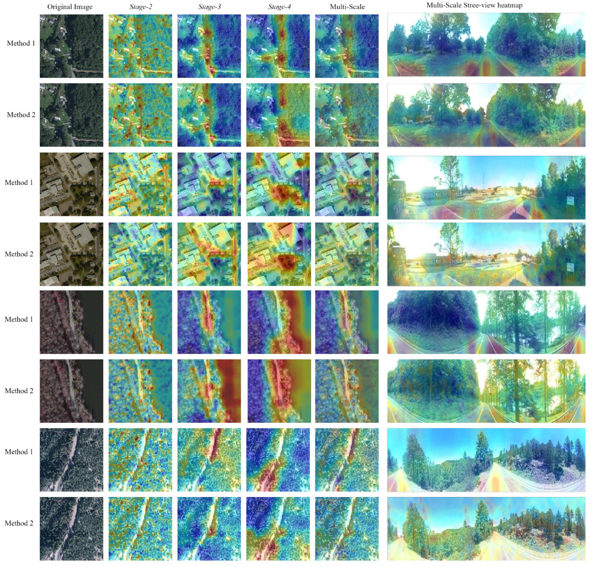
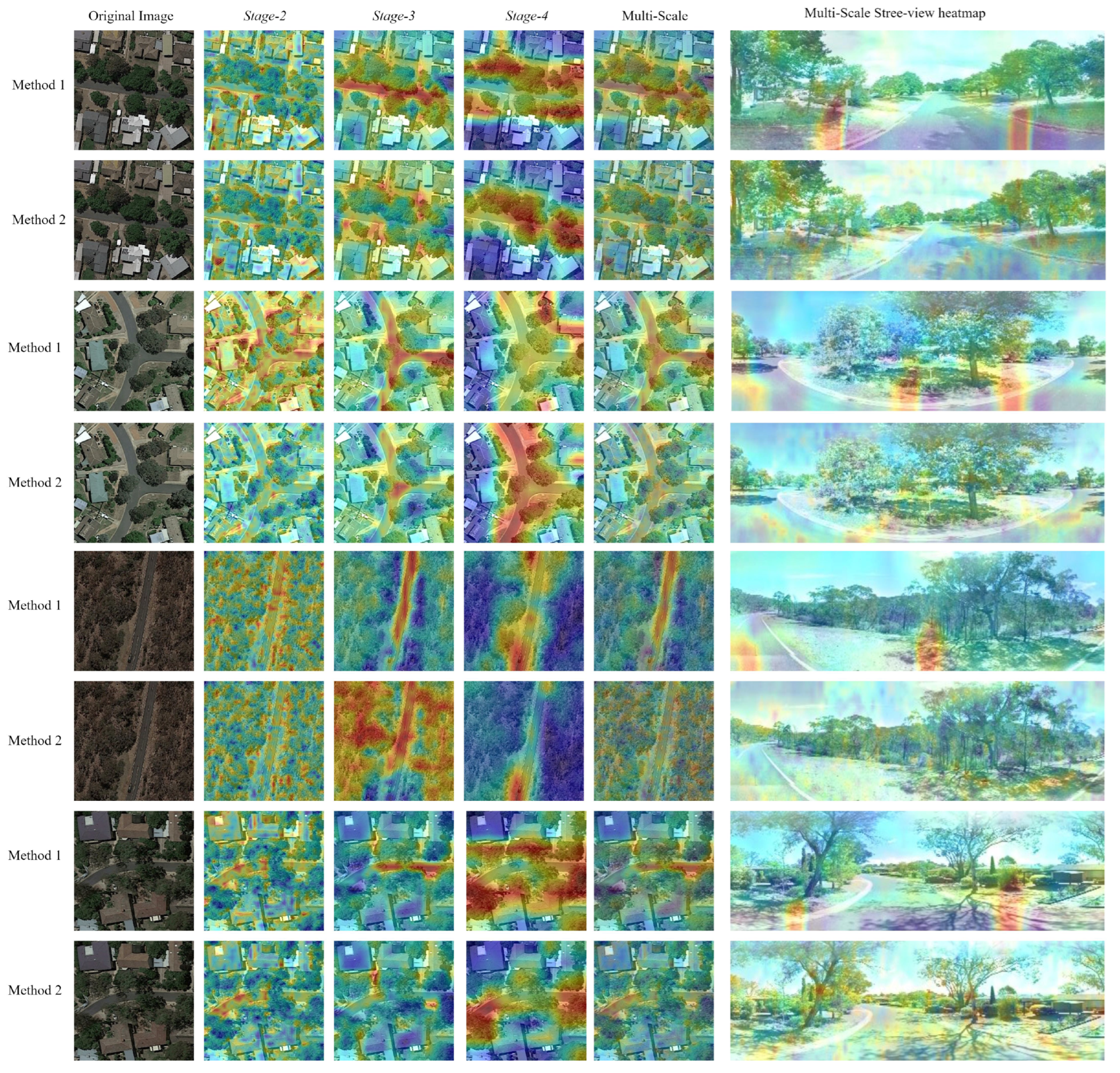
22]. Specifically, we average the features along the channel dimension, resize them to the original image size, and overlay them on the original image to generate the heatmap. It is noteworthy that, due to the different fields of view and perspectives between street-view images and RS images, street-view images may contain significant occlusions. This implies that areas closer to the center of the RS image and regions that are not occluded are more likely to appear in the street-view image. Therefore, to achieve better performance, the model should pay more attention to areas that appear in both images. This implies that these regions should have higher thermal values, while other areas should have lower thermal values.
As shown in
Figure 8 and
Figure 9, whether under “Method 1” or “Method 2”, the heatmap of Stage-2 exhibits a scattered distribution of high thermal values in a dot pattern with fewer low thermal value areas and slight differences in the thermal values. In contrast, in the heatmaps of Stage-3 and Stage-4, high thermal values are distributed in a patchy pattern around the center of the image (the location where the street-view image is captured) and its surrounding areas with more areas with low thermal values and greater differences in the thermal values. The distribution of the high thermal values in Stage-3 and Stage-4 indicates that the features at these stages focus on information relevant to our task while reducing attention given to irrelevant information. In the heatmaps from Stage-3 and Stage-4, the higher thermal values are in the center of the images as well as in non-occluded areas. This indicates that the model focuses on important and valuable areas. In contrast, the heatmaps from Stage-2 do not exhibit this phenomenon and high thermal values appear in several occluded areas and boundary regions. Additionally, the distribution of the high thermal values in Stage-3 and Stage-4 varies, indicating that they can focus on different valuable areas.
By simultaneously using features from both Stage-3 and Stage-4 as our multi-scale features, our model can focus on larger valuable regions while retaining attention on the image’s central region and non-occluded areas. This is consistent with the objective of utilizing multi-scale features and clarifies the improvement in our model’s performance when incorporating features from Stage-3 and Stage-4 as part of the multi-scale features. Meanwhile, the scattered distribution of the high thermal values in Stage-2 suggests that the features in this stage have not adequately extracted crucial information, and the module emphasizes occluded areas, which are not visible in the street-view images. When incorporating the features from Stage-2 into the multi-scale features, the regions with high thermal values in the heatmap are suppressed, and the areas with low thermal values decrease. The overall thermal values in the image show a trend toward a more even distribution. When features from Stage-2 are included as part of the multi-scale features, the thermal values in the heatmap exhibit an even distribution trend. This suggests that the inclusion of Stage-2 features leads the model to reduce attention to valuable information and focus more on a broader range of less valuable information. This aligns with our experimental results, showing that using features from Stage-2, Stage-3, and Stage-4 as our multi-scale features does not improve model performance.
The same phenomenon can be observed in the heatmaps of the street-view images. The heatmaps of the street-view images, composed of features from Stage-3 and Stage-4 as the multi-scale features, exhibit more pronounced high thermal values regions. In contrast, the heatmaps of the street-view images, composed of features from Stage-2, Stage-3, and Stage-4 as the multi-scale features, show masked high thermal value regions, presenting a more uniform distribution of thermal values. Simultaneously, when using features from Stage-3 and Stage-4 to compose multi-scale features, the high thermal value regions in the heatmaps of the street-view images and RS images show a more evident correspondence. This indicates that the model is focusing on the same areas in both the street-view images and RS images, contributing to the extraction of valuable features from them. Yet, this correspondence is challenging to discern when using features from Stage-2, Stage-3, and Stage-4 to compose multi-scale features.
Through the heatmap visualization of features at different scales, we observed variations in the regions of focus within the images. Our model exhibits distinct performances when composed of features from different stages to form multi-scale features. Using features from Stage-3 and Stage-4 to compose the multi-scale features, our model can focus on a larger extent of the prominent regions that appear simultaneously in both the street-view images and RS images, enhancing model performance. Conversely, due to the scattered distribution of the high thermal values in the heatmaps, the multi-scale features composed of features from Stage-2, Stage-3, and Stage-4, intuitively expected to contain more information, do not yield a performance improvement. By selecting appropriate features, our model demonstrates better performance.
6. Conclusions
In this paper, we proposed a lightweight end-to-end method for cross-view geo-localization. Specifically, to enable the model to focus on more diverse features, we extract features of different scales from different stages of our model to obtain multi-scale features. Simultaneously, to strengthen the robustness of extracting and aligning meaningful multi-scale features, we introduce contrastive learning to our model during the training process. Our model exhibits performance surpassing the state-of-the-art models while demanding fewer computational resources than other end-to-end methods. On the CVUSA and CVACT datasets, our model achieved a 1.42% and 4.67% improvement in , 0.86% and 1.79% improvement in , 0.63% and 1.14% improvement in , and 0.006% and 0.11% improvement in , respectively. In the first type of meter-level evaluation, our method achieved 4.80%, 3.71%, 3.41%, and 3.31% absolute improvements in the 0 m, 36 m, 72 m, and 144 m thresholds, respectively. In the second type of meter-lever evaluation, our model achieved the smallest average distance between the retrieval results and the ground-truth images. Additionally, compared to other end-to-end models, our model reduces the GFLOPs, parameter count, and inference time by at least 75%, 65%, and 29%, respectively. The improvement efficiency of our model will facilitate the widespread application of cross-view geo-localization technology to large-scale practical scenarios.
Overall, our method boasts higher accuracy and lower computational costs. In the future, we will explore cross-view geo-localization technology from a more practical perspective. On the one hand, addressing the challenge of inconsistencies in the center points and orientations between RS images and street-view images will be a primary focus of further research. This discrepancy presents significant challenges for cross-view geo-localization technology in practical applications. On the other hand, compared to street-view images, photos captured by ordinary cameras are more readily available in practical applications. Cross-view geo-localization technology for such photo images holds broader prospects. Therefore, we will conduct research on cross-view geo-localization problems specific to this type of photo image in the future.
Author Contributions
Conceptualization, methodology, investigation, data curation, formal analysis, and writing—original draft preparation, W.Z.; conceptualization, methodology, investigation, and writing—review and editing, H.C. Supervision, H.C., Z.Z. and N.J. All the authors read, edited, and critiqued the manuscript and approved the final version. All authors have read and agreed to the published version of the manuscript.
Funding
This work was supported in part by the National NSF of China under grants No. U19A2058, No. 41971362, No. 41871248, and No. 62106276.
Data Availability Statement
This study did not report any data.
Acknowledgments
The authors would like to thank the anonymous referees for their valuable comments and helpful suggestions.
Conflicts of Interest
The authors declare no conflicts of interest.
References
- Wang, S.; Cao, J.; Philip, S.Y. Deep learning for spatio-temporal data mining: A survey. IEEE Trans. Knowl. Data Eng. 2020, 34, 3681–3700. [Google Scholar] [CrossRef]
- Chen, H.; Li, Z.; Wu, J.; Xiong, W.; Du, C. SemiRoadExNet: A semi-supervised network for road extraction from remote sensing imagery via adversarial learning. ISPRS J. Photogramm. Remote Sens. 2023, 198, 169–183. [Google Scholar] [CrossRef]
- Sun, C.; Wu, J.; Chen, H.; Du, C. SemiSANet: A semi-supervised high-resolution remote sensing image change detection model using Siamese networks with graph attention. Remote Sens. 2022, 14, 2801. [Google Scholar] [CrossRef]
- Brosh, E.; Friedmann, M.; Kadar, I.; Yitzhak Lavy, L.; Levi, E.; Rippa, S.; Lempert, Y.; Fernandez-Ruiz, B.; Herzig, R.; Darrell, T. Accurate visual localization for automotive applications. In Proceedings of the IEEE/CVF Conference on Computer Vision and Pattern Recognition Workshops, Long Beach, CA, USA, 15–20 June 2019. [Google Scholar]
- Wang, T.; Zheng, Z.; Yan, C.; Zhang, J.; Sun, Y.; Zheng, B.; Yang, Y. Each part matters: Local patterns facilitate cross-view geo-localization. IEEE Trans. Circuits Syst. Video Technol. 2021, 32, 867–879. [Google Scholar] [CrossRef]
- Zhu, S.; Yang, T.; Chen, C. Vigor: Cross-view image geo-localization beyond one-to-one retrieval. In Proceedings of the IEEE/CVF Conference on Computer Vision and Pattern Recognition, Nashville, TN, USA, 20–25 June 2021; pp. 3640–3649. [Google Scholar]
- Weyand, T.; Kostrikov, I.; Philbin, J. Planet-photo geolocation with convolutional neural networks. In Proceedings of the Computer Vision—ECCV 2016: 14th European Conference, Amsterdam, The Netherlands, 11–14 October 2016; Proceedings, Part VIII 14. Springer: Berlin/Heidelberg, Germany, 2016; pp. 37–55. [Google Scholar]
- Sun, B.; Chen, C.; Zhu, Y.; Jiang, J. Geocapsnet: Ground to aerial view image geo-localization using capsule network. In Proceedings of the 2019 IEEE International Conference on Multimedia and Expo (ICME), Shanghai, China, 8–12 July 2019; pp. 742–747. [Google Scholar]
- Hu, S.; Feng, M.; Nguyen, R.M.; Lee, G.H. Cvm-net: Cross-view matching network for image-based ground-to-aerial geo-localization. In Proceedings of the IEEE Conference on Computer Vision and Pattern Recognition, Salt Lake City, UT, USA, 18–23 June 2018; pp. 7258–7267. [Google Scholar]
- Liu, L.; Li, H. Lending orientation to neural networks for cross-view geo-localization. In Proceedings of the IEEE/CVF Conference on Computer Vision and Pattern Recognition, Long Beach, CA, USA, 15–20 June 2019; pp. 5624–5633. [Google Scholar]
- Xu, Y.; Wu, S.; Du, C.; Li, J.; Jing, N. UAV Image Geo-Localization by Point-Line-Patch Feature Matching and ICLK Optimization. In Proceedings of the 2022 29th International Conference on Geoinformatics, Beijing, China, 15–18 August 2022. [Google Scholar] [CrossRef]
- Shi, Y.; Liu, L.; Yu, X.; Li, H. Spatial-aware feature aggregation for image based cross-view geo-localization. Adv. Neural Inf. Process. Syst. 2019, 32. [Google Scholar]
- Tian, Y.; Chen, C.; Shah, M. Cross-view image matching for geo-localization in urban environments. In Proceedings of the IEEE Conference on Computer Vision and Pattern Recognition, Honolulu, HI, USA, 21–26 July 2017; pp. 3608–3616. [Google Scholar]
- Zhu, S.; Yang, T.; Chen, C. Revisiting street-to-aerial view image geo-localization and orientation estimation. In Proceedings of the IEEE/CVF Winter Conference on Applications of Computer Vision, Waikoloa, HI, USA, 3–8 January 2021; pp. 756–765. [Google Scholar]
- Shi, Y.; Yu, X.; Campbell, D.; Li, H. Where am i looking at? joint location and orientation estimation by cross-view matching. In Proceedings of the IEEE/CVF Conference on Computer Vision and Pattern Recognition, Seattle, WA, USA, 13–19 June 2020; pp. 4064–4072. [Google Scholar]
- Vo, N.N.; Hays, J. Localizing and orienting street views using overhead imagery. In Proceedings of the Computer Vision—ECCV 2016: 14th European Conference, Amsterdam, The Netherlands, 11–14 October 2016; Proceedings, Part I 14. Springer: Berlin/Heidelberg, Germany, 2016; pp. 494–509. [Google Scholar]
- Mirza, M.; Osindero, S. Conditional generative adversarial nets. arXiv 2014, arXiv:1411.1784. [Google Scholar]
- Lu, X.; Li, Z.; Cui, Z.; Oswald, M.R.; Pollefeys, M.; Qin, R. Geometry-aware satellite-to-ground image synthesis for urban areas. In Proceedings of the IEEE/CVF Conference on Computer Vision and Pattern Recognition, Seattle, WA, USA, 13–19 June 2020; pp. 859–867. [Google Scholar]
- Regmi, K.; Borji, A. Cross-view image synthesis using conditional gans. In Proceedings of the IEEE Conference on Computer Vision and Pattern Recognition, Salt Lake City, UT, USA, 18–23 June 2018; pp. 3501–3510. [Google Scholar]
- Toker, A.; Zhou, Q.; Maximov, M.; Leal-Taixé, L. Coming down to earth: Satellite-to-street view synthesis for geo-localization. In Proceedings of the IEEE/CVF Conference on Computer Vision and Pattern Recognition, Nashville, TN, USA, 20–25 June 2021; pp. 6488–6497. [Google Scholar]
- Dosovitskiy, A.; Beyer, L.; Kolesnikov, A.; Weissenborn, D.; Zhai, X.; Unterthiner, T.; Dehghani, M.; Minderer, M.; Heigold, G.; Gelly, S.; et al. An image is worth 16x16 words: Transformers for image recognition at scale. arXiv 2020, arXiv:2010.11929. [Google Scholar]
- Dai, M.; Hu, J.; Zhuang, J.; Zheng, E. A transformer-based feature segmentation and region alignment method for UAV-view geo-localization. IEEE Trans. Circuits Syst. Video Technol. 2021, 32, 4376–4389. [Google Scholar] [CrossRef]
- Zhu, S.; Shah, M.; Chen, C. Transgeo: Transformer is all you need for cross-view image geo-localization. In Proceedings of the IEEE/CVF Conference on Computer Vision and Pattern Recognition, New Orleans, LA, USA, 18–24 June 2022; pp. 1162–1171. [Google Scholar]
- Pramanick, S.; Nowara, E.M.; Gleason, J.; Castillo, C.D.; Chellappa, R. Where in the world is this image? transformer-based geo-localization in the wild. In Proceedings of the European Conference on Computer Vision, Tel Aviv, Israel, 23–27 October 2022; Springer: Berlin/Heidelberg, Germany, 2022; pp. 196–215. [Google Scholar]
- Liu, Z.; Lin, Y.; Cao, Y.; Hu, H.; Wei, Y.; Zhang, Z.; Lin, S.; Guo, B. Swin transformer: Hierarchical vision transformer using shifted windows. In Proceedings of the IEEE/CVF International Conference on Computer Vision, Montreal, BC, Canada, 11–17 October 2021; pp. 10012–10022. [Google Scholar]
- Wu, Z.; Xiong, Y.; Yu, S.X.; Lin, D. Unsupervised feature learning via non-parametric instance discrimination. In Proceedings of the IEEE Conference on Computer Vision and Pattern Recognition, Salt Lake City, UT, USA, 18–23 June 2018; pp. 3733–3742. [Google Scholar]
- Chen, T.; Kornblith, S.; Norouzi, M.; Hinton, G. A simple framework for contrastive learning of visual representations. In Proceedings of the International Conference on Machine Learning, PMLR, Online, 13–18 July 2020; pp. 1597–1607. [Google Scholar]
- Agarwal, S.; Furukawa, Y.; Snavely, N.; Simon, I.; Curless, B.; Seitz, S.M.; Szeliski, R. Building rome in a day. Commun. ACM 2011, 54, 105–112. [Google Scholar] [CrossRef]
- Zamir, A.R.; Shah, M. Accurate image localization based on google maps street view. In Proceedings of the Computer Vision—ECCV 2010: 11th European Conference on Computer Vision, Heraklion, Crete, Greece, 5–11 September 2010; Proceedings, Part IV 11. Springer: Berlin/Heidelberg, Germany, 2010; pp. 255–268. [Google Scholar]
- Baatz, G.; Saurer, O.; Köser, K.; Pollefeys, M. Large scale visual geo-localization of images in mountainous terrain. In Proceedings of the Computer Vision—ECCV 2012: 12th European Conference on Computer Vision, Florence, Italy, 7–13 October 2012; Proceedings, Part II 12. Springer: Berlin/Heidelberg, Germany, 2012; pp. 517–530. [Google Scholar]
- Lin, T.Y.; Belongie, S.; Hays, J. Cross-view image geolocalization. In Proceedings of the IEEE Conference on Computer Vision and Pattern Recognition, Portland, OR, USA, 23–28 June 2013; pp. 891–898. [Google Scholar]
- Workman, S.; Souvenir, R.; Jacobs, N. Wide-area image geolocalization with aerial reference imagery. In Proceedings of the IEEE International Conference on Computer Vision, Santiago, Chile, 7–13 December 2015; pp. 3961–3969. [Google Scholar]
- Regmi, K.; Shah, M. Bridging the domain gap for ground-to-aerial image matching. In Proceedings of the IEEE/CVF International Conference on Computer Vision, Seoul, Republic of Korea, 27 October–2 November 2019; pp. 470–479. [Google Scholar]
- Shi, Y.; Yu, X.; Liu, L.; Zhang, T.; Li, H. Optimal feature transport for cross-view image geo-localization. In Proceedings of the AAAI Conference on Artificial Intelligence, New York, NY, USA, 7–12 February 2020; Volume 34, pp. 11990–11997. [Google Scholar]
- Yang, H.; Lu, X.; Zhu, Y. Cross-view geo-localization with layer-to-layer transformer. Adv. Neural Inf. Process. Syst. 2021, 34, 29009–29020. [Google Scholar]
- Touvron, H.; Cord, M.; Douze, M.; Massa, F.; Sablayrolles, A.; Jégou, H. Training data-efficient image transformers & distillation through attention. In Proceedings of the International Conference on Machine Learning, PMLR, Online, 18–24 July 2021; pp. 10347–10357. [Google Scholar]
- Liu, Z.; Tan, Y.; He, Q.; Xiao, Y. SwinNet: Swin transformer drives edge-aware RGB-D and RGB-T salient object detection. IEEE Trans. Circuits Syst. Video Technol. 2021, 32, 4486–4497. [Google Scholar] [CrossRef]
- Li, Z.; Chen, H.; Jing, N.; Li, J. RemainNet: Explore Road Extraction from Remote Sensing Image Using Mask Image Modeling. Remote Sens. 2023, 15, 4215. [Google Scholar] [CrossRef]
- Liang, J.; Cao, J.; Sun, G.; Zhang, K.; Van Gool, L.; Timofte, R. Swinir: Image restoration using swin transformer. In Proceedings of the IEEE/CVF International Conference on Computer Vision, Montreal, BC, Canada, 11–17 October 2021; pp. 1833–1844. [Google Scholar]
- Vaswani, A.; Shazeer, N.; Parmar, N.; Uszkoreit, J.; Jones, L.; Gomez, A.N.; Kaiser, Ł.; Polosukhin, I. Attention is all you need. Adv. Neural Inf. Process. Syst. 2017, 30. [Google Scholar]
- Chen, T.; Kornblith, S.; Swersky, K.; Norouzi, M.; Hinton, G.E. Big self-supervised models are strong semi-supervised learners. Adv. Neural Inf. Process. Syst. 2020, 33, 22243–22255. [Google Scholar]
- He, K.; Fan, H.; Wu, Y.; Xie, S.; Girshick, R. Momentum contrast for unsupervised visual representation learning. In Proceedings of the IEEE/CVF Conference on Computer Vision and Pattern Recognition, Seattle, WA, USA, 13–19 June 2020; pp. 9729–9738. [Google Scholar]
- Zhang, H.; Li, F.; Liu, S.; Zhang, L.; Su, H.; Zhu, J.; Ni, L.M.; Shum, H.Y. Dino: Detr with improved denoising anchor boxes for end-to-end object detection. arXiv 2022, arXiv:2203.03605. [Google Scholar]
- Chen, X.; Xie, S.; He, K. An empirical study of training self-supervised vision transformers. In Proceedings of the CVF International Conference on Computer Vision (ICCV), Montreal, BC, Canada, 11–17 October 2021; pp. 9620–9629. [Google Scholar]
- Zhai, M.; Bessinger, Z.; Workman, S.; Jacobs, N. Predicting ground-level scene layout from aerial imagery. In Proceedings of the IEEE Conference on Computer Vision and Pattern Recognition, Honolulu, HI, USA, 21–26 July 2017; pp. 867–875. [Google Scholar]
- Paszke, A.; Gross, S.; Massa, F.; Lerer, A.; Bradbury, J.; Chanan, G.; Killeen, T.; Lin, Z.; Gimelshein, N.; Antiga, L.; et al. Pytorch: An imperative style, high-performance deep learning library. Adv. Neural Inf. Process. Syst. 2019, 32. [Google Scholar]
- Liu, Z.; Hu, H.; Lin, Y.; Yao, Z.; Xie, Z.; Wei, Y.; Ning, J.; Cao, Y.; Zhang, Z.; Dong, L.; et al. Swin transformer v2: Scaling up capacity and resolution. In Proceedings of the IEEE/CVF Conference on Computer Vision and Pattern Recognition, New Orleans, LA, USA, 18–24 July 2022; pp. 12009–12019. [Google Scholar]
- Deng, J.; Dong, W.; Socher, R.; Li, L.J.; Li, K.; Fei-Fei, L. Imagenet: A large-scale hierarchical image database. In Proceedings of the 2009 IEEE Conference on Computer Vision and Pattern Recognition, Miami, FL, USA, 20–25 June 2009; pp. 248–255. [Google Scholar]
- Loshchilov, I.; Hutter, F. Decoupled weight decay regularization. arXiv 2017, arXiv:1711.05101. [Google Scholar]
- Loshchilov, I.; Hutter, F. Sgdr: Stochastic gradient descent with warm restarts. arXiv 2016, arXiv:1608.03983. [Google Scholar]
- Kwon, J.; Kim, J.; Park, H.; Choi, I.K. Asam: Adaptive sharpness-aware minimization for scale-invariant learning of deep neural networks. In Proceedings of the International Conference on Machine Learning, PMLR, Online, 18–24 July 2021; pp. 5905–5914. [Google Scholar]
Figure 1.
The process of cross-view geo-localization.
Figure 1.
The process of cross-view geo-localization.
Figure 2.
An overview of GeoViewMatch. The “↔” means shared weights. The “
”, “
”, and “
” are the loss functions for training our model, see
Section 3.4.
Figure 2.
An overview of GeoViewMatch. The “↔” means shared weights. The “
”, “
”, and “
” are the loss functions for training our model, see
Section 3.4.
Figure 3.
The structure of Swin-Geo. The “ST Stage” is the stage in swin-transformer. The symbol “⊗” means concatenation. FA is a feature aggregation module, see
Figure 4.
Figure 3.
The structure of Swin-Geo. The “ST Stage” is the stage in swin-transformer. The symbol “⊗” means concatenation. FA is a feature aggregation module, see
Figure 4.
Figure 4.
Feature aggregation module. “⊗” and “⊙” are mean concatenation and Frobenius inner product, respectively.
Figure 4.
Feature aggregation module. “⊗” and “⊙” are mean concatenation and Frobenius inner product, respectively.
Figure 5.
The rotation of RS image and corresponding transformation of street-view image.
Figure 5.
The rotation of RS image and corresponding transformation of street-view image.
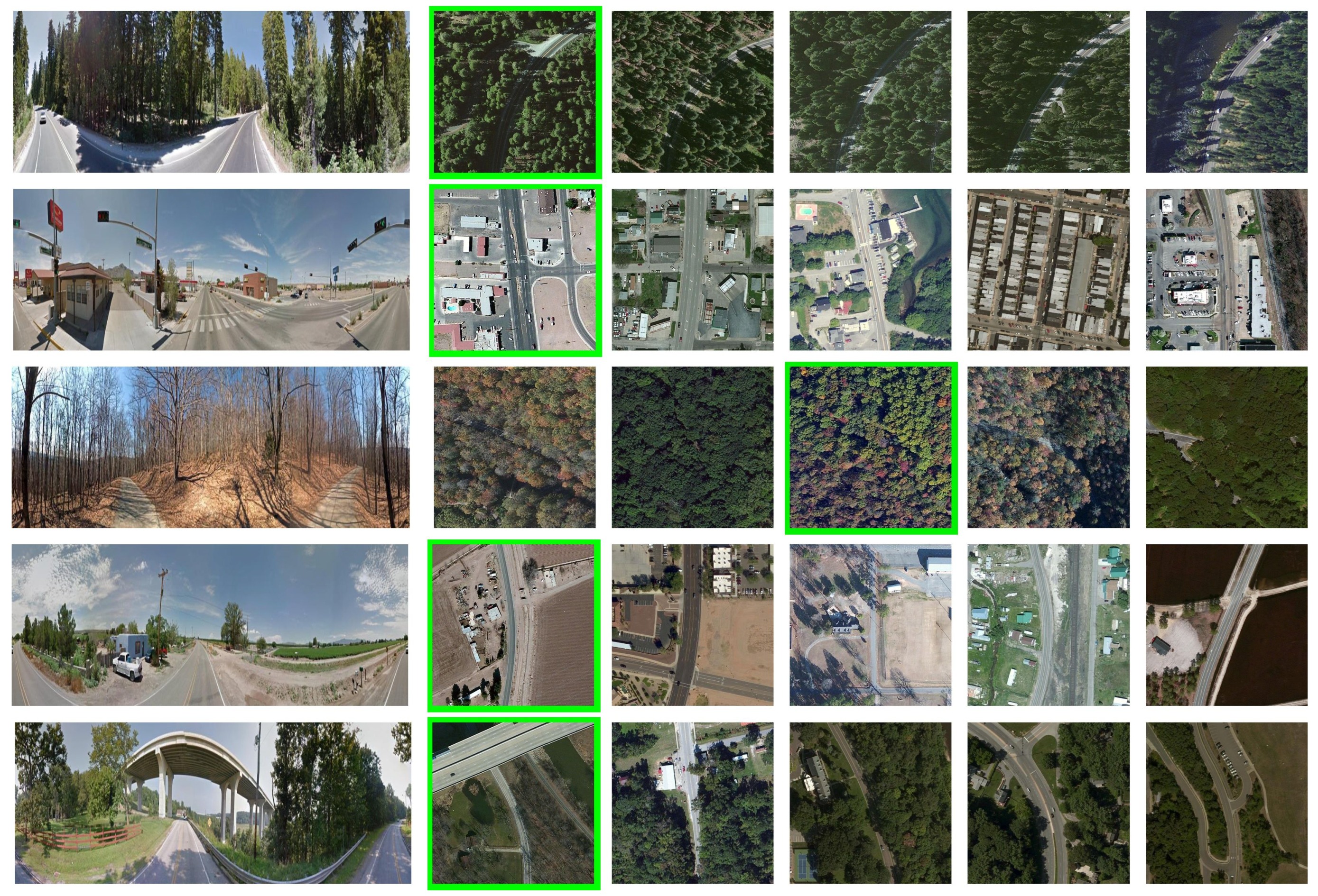
Figure 6.
The retrieval results under the CVUSA dataset. The left side shows the street-view images, and the right side displays the top five retrieval results sorted by similarity from high to low. The green boxes indicate the correct retrieval results.
Figure 6.
The retrieval results under the CVUSA dataset. The left side shows the street-view images, and the right side displays the top five retrieval results sorted by similarity from high to low. The green boxes indicate the correct retrieval results.
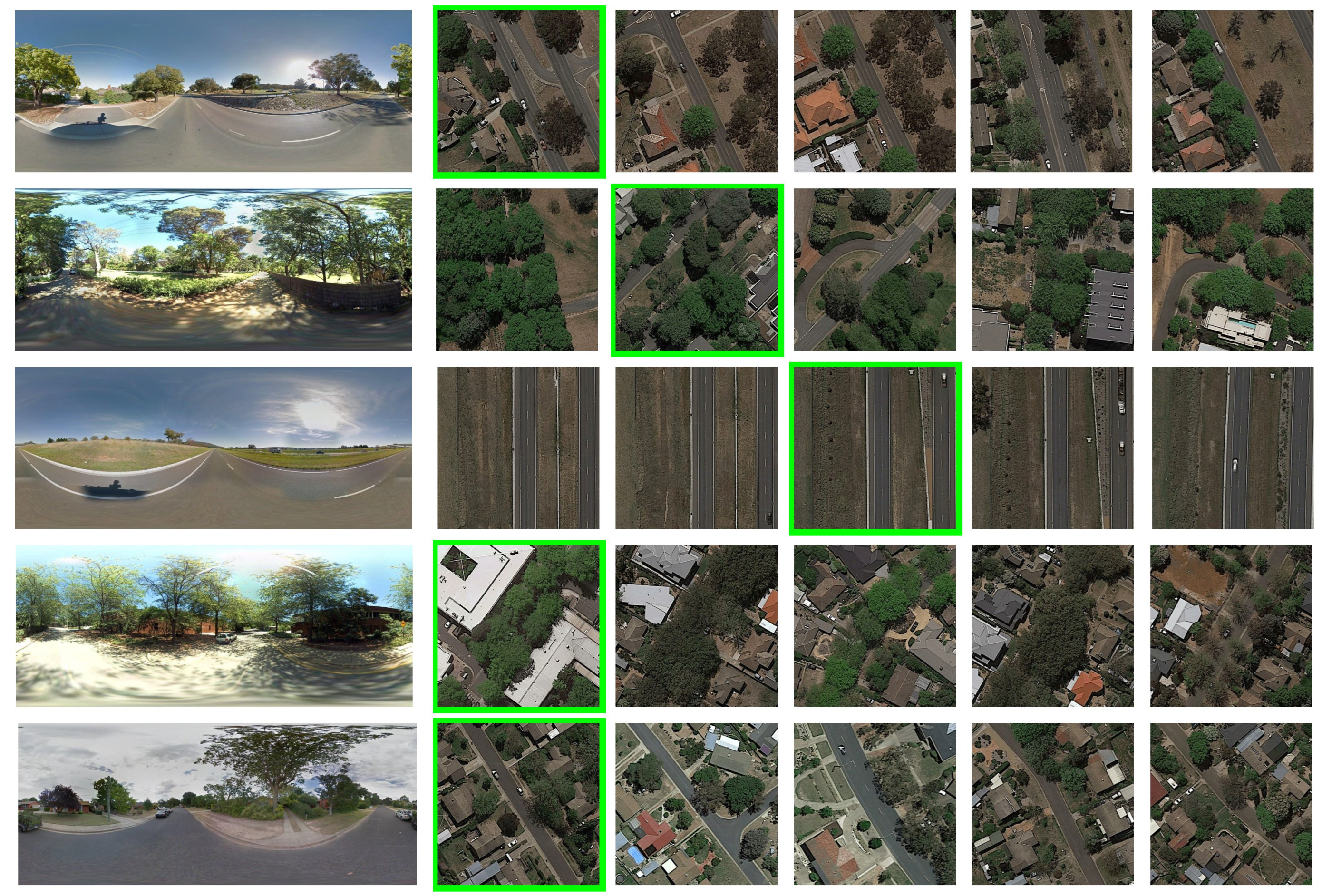
Figure 7.
The retrieval results under the CVACT dataset. The left side shows the street-view images, and the right side displays the top five retrieval results sorted by similarity from high to low. The green boxes indicate the correct retrieval results.
Figure 7.
The retrieval results under the CVACT dataset. The left side shows the street-view images, and the right side displays the top five retrieval results sorted by similarity from high to low. The green boxes indicate the correct retrieval results.
Figure 8.
The heatmaps from the CVUSA dataset. On the left, the original RS images are shown, and on the right are four heatmaps from Stage-2, Stage-3, and Stage-4 of Swin-Geo, along with heatmaps from the multi-scale features. The far right displays the heatmaps of the multi-scale feature extracted from the street-view images. “Method 1” denotes the use of features from Stage-3 and Stage-4 of Swin-Geo to form multi-scale features, while “Method 2” indicates the use of features from Stage-2, Stage-3, and Stage-4 of Swin-Geo to compose multi-scale features. Red represents high thermal values in this area, while blue represents low thermal values.
Figure 9.
The heatmaps from the CVACT dataset. On the left, the original RS images are shown, and on the right are four heatmaps from Stage-2, Stage-3, and Stage-4 of Swin-Geo, along with the heatmaps from the multi-scale features. The far right displays the heatmaps of the multi-scale feature extracted from the street-view images. “Method 1” denotes the use of features from Stage-3 and Stage-4 of Swin-Geo to form multi-scale features, while “Method 2” indicates the use of features from Stage-2, Stage-3, and Stage-4 of Swin-Geo to compose multi-scale features. Red represents high thermal values in this area, while blue represents low thermal values.
Table 1.
Comparison of , , , and on the CVUSA and CVACT datasets. (The best is in bold).
Table 1.
Comparison of , , , and on the CVUSA and CVACT datasets. (The best is in bold).
| | CVUSA | CVACT |
|---|
| Method | | | | | | | | % |
| LOCG | 40.79 | 68.82 | 76.36 | 96.12 | 46.96 | 68.28 | 75.48 | 92.01 |
| CVTF | 61.43 | 84.69 | 90.49 | 99.02 | 61.05 | 81.33 | 86.52 | 95.93 |
| SAFA | 89.84 | 96.93 | 98.14 | 99.64 | 81.03 | 92.80 | 94.84 | 98.17 |
| CDTE | 92.56 | 97.55 | 98.33 | 99.57 | 83.28 | 93.57 | 95.42 | 98.22 |
| L2LTR | 94.05 | 98.27 | 98.99 | 99.67 | 84.89 | 94.59 | 95.96 | 98.37 |
| TransGeo | 94.08 | 98.36 | 99.04 | 99.77 | 84.95 | 94.14 | 95.78 | 98.37 |
| GeoViewMatch | 95.52 | 99.22 | 99.67 | 99.83 | 89.71 | 95.93 | 96.92 | 98.48 |
Table 2.
Results at thresholds of 0, 36, 72, and 144 on the CVACT dataset. (The best is in bold).
Table 2.
Results at thresholds of 0, 36, 72, and 144 on the CVACT dataset. (The best is in bold).
| | Threshold (m) |
|---|
| Method | 0 | 36 | 72 | 144 |
| LOCG | 42.13 | 44.23 | 45.04 | 46.34 |
| CVTF | 59.35 | 64.66 | 65.75 | 67.51 |
| SAFA | 72.76 | 77.75 | 78.69 | 79.92 |
| CDTE | 83.44 | 88.97 | 89.77 | 90.69 |
| L2LTR | 83.91 | 88.99 | 89.97 | 90.83 |
| TransGeo | 84.91 | 89.59 | 90.42 | 91.19 |
| GeoViewMatch | 89.71 | 93.30 | 93.83 | 94.50 |
Table 3.
The average distance between the top-k retrieval results and the ground-truth image on the CVACT dataset. (The best is in bold).
Table 3.
The average distance between the top-k retrieval results and the ground-truth image on the CVACT dataset. (The best is in bold).
| | Distance (m) |
|---|
| Method | Top-1 | Top-5 | Top-10 | Top-1% |
| LOCG | 2546 | 3859 | 4215 | 4909 |
| CVTF | 1378 | 3396 | 3939 | 4894 |
| SAFA | 916 | 3238 | 3882 | 4953 |
| CDTE | 392 | 2911 | 3594 | 4778 |
| L2LTR | 384 | 2938 | 3671 | 4876 |
| TransGeo | 352 | 2821 | 3556 | 4790 |
| GeoViewMatch | 223 | 2668 | 3403 | 4700 |
Table 4.
The GFLOPs, GPU memory, inference speed, parameter, and performance on the CVACT dataset. All three methods are tested on the same RTX4090 with a batch size of 16. (The best is in bold).
Table 4.
The GFLOPs, GPU memory, inference speed, parameter, and performance on the CVACT dataset. All three methods are tested on the same RTX4090 with a batch size of 16. (The best is in bold).
| Method | GFLOPs | GPU Memory | Inference Time | Parameter | |
|---|
| SAFA | 42.24 | 9.63 GB | 120 ms | 81.66 | 81.03 |
| L2LTR | 44.16 | 15.50 GB | 82 ms | 195.90 | 84.89 |
| GeoViewMatch | 9.7616 | 11.40 GB | 42 ms | 57.47 | 89.71 |
Table 5.
The ablation results for the CVUSA and CVACT datasets. The abbreviations “BS”, “CL”, and “MF” represent the base model, contrastive learning, and multi-scale features, respectively. (The best is in bold).
Table 5.
The ablation results for the CVUSA and CVACT datasets. The abbreviations “BS”, “CL”, and “MF” represent the base model, contrastive learning, and multi-scale features, respectively. (The best is in bold).
| Dataset | Method | | | | |
|---|
| CVUSA | BS | 94.99 | 98.53 | 99.71 | 99.84 |
| BS + CL | 95.28 | 98.77 | 99.20 | 99.81 |
| BS + MF | 95.32 | 98.81 | 99.31 | 99.82 |
| BS + CL + MF | 95.52 | 99.22 | 99.67 | 99.83 |
| CVACT | BS | 88.65 | 95.27 | 96.67 | 98.39 |
| BS + CL | 89.17 | 95.81 | 96.92 | 98.41 |
| BS + MF | 89.25 | 95.67 | 96.59 | 98.41 |
| BS + CL + MF | 89.71 | 95.93 | 96.92 | 98.48 |
Table 6.
The performance of our model under various multi-scale features. The symbols , , , and denote the out features of Stage-4, Stage-3, Stage-2, and Stage-1 of Swin-Geo, respectively. The symbol ⊗ means concatenation. means using the multi-scale features composed of the features and . (The best is in bold).
| Dataset | Method | | | | |
|---|
| CVUSA | | 95.28 | 98.77 | 99.20 | 99.81 |
| 95.52 | 99.22 | 99.67 | 99.83 |
| 95.38 | 98.68 | 99.25 | 99.81 |
| 50.11 | 71.65 | 78.18 | 91.86 |
| CVACT | | 89.17 | 95.81 | 96.92 | 98.41 |
| 89.71 | 95.93 | 96.92 | 98.48 |
| 89.25 | 95.67 | 96.57 | 98.39 |
| 35.12 | 59.06 | 68.66 | 91.37 |
| Disclaimer/Publisher’s Note: The statements, opinions and data contained in all publications are solely those of the individual author(s) and contributor(s) and not of MDPI and/or the editor(s). MDPI and/or the editor(s) disclaim responsibility for any injury to people or property resulting from any ideas, methods, instructions or products referred to in the content. |
© 2024 by the authors. Licensee MDPI, Basel, Switzerland. This article is an open access article distributed under the terms and conditions of the Creative Commons Attribution (CC BY) license (https://creativecommons.org/licenses/by/4.0/).


