Retrieval of Surface Energy Fluxes Considering Vegetation Changes and Aerosol Effects

Abstract

The exchange of moisture and energy between the land and the atmosphere plays a crucial role in terrestrial hydrological cycle and climate change. However, existing studies on the retrieval of surface water and heat flux tend to overlook the dynamic changes in surface vegetation and atmospheric aerosols, which directly affect surface energy and indirectly alter various meteorological factors, including cloud, precipitation, and temperature. In this study, we assess the machine-learning retrieval method for surface fluxes that takes into account vegetation changes and aerosol effects, using FLUXNET observations and remote sensing data to retrieve latent heat flux (LE) and sensible heat flux (H). We constructed four sets of deep neural network models: (a) The first set considers only meteorological factors, (b) the second set considers meteorological factors and aerosols, (c) the third set considers meteorological factors and vegetation changes, and (d) the fourth set comprehensively considers meteorological factors, aerosols, and vegetation changes. All model performances were evaluated using statistical indicators. ERA5 reanalysis and remote sensing data were used to drive the models and retrieve daily H and LE. The retrieved results were validated against ground observation sites that were not involved in model training or the FLUXCOM product. The results show that the model that considers meteorological factors, aerosols, and vegetation changes has the smallest errors and highest correlation for retrieving H and LE (R_H = 0.85, RMSE_H = 24.88; R_LE = 0.88, RMSE_LE = 22.25). The ability of the four models varies under different vegetation types. In terms of seasons, the models that consider meteorological factors and vegetation changes, as well as those that comprehensively consider meteorological factors, aerosols, and vegetation changes, perform well in retrieving the surface fluxes. As for spatial distribution, when atmospheric aerosols are present in the region, the model that considers both meteorological factors and aerosols retrieves higher values of H compared to the model that considers only meteorological factors, while the LE values are relatively lower. The model that considers meteorological factors and vegetation changes, as well as the model that comprehensively considers meteorological factors, aerosols, and vegetation changes, retrieves lower values in most regions. Through the validation of independent observation sites and FLUXCOM products, we found that the model, considering meteorological factors, aerosols, and vegetation changes, was generally more accurate in the retrieval of surface fluxes. This study contributes to improving the retrieval and future prediction accuracy of surface fluxes in a changing environment.

1. Introduction

Changes in the terrestrial water and energy balance are the primary drivers of global climate variability and change. These changes can lead to frequent and severe extreme weather and climate events, such as heat waves and droughts [1,2,3]. Monitoring the spatial and temporal patterns of surface energy fluxes is important to better understand the water cycle and climate change [4,5,6,7]. Therefore, it is particularly important to accurately estimate surface water and heat fluxes and to study their evolutionary patterns in a changing environment.

Surface water and heat fluxes consist of two main components: Latent heat flux (LE) and sensible heat flux (H). Changes in LE and H are generally influenced by a combination of various environmental factors, such as vegetation, meteorological elements, and human activities [8,9,10]. Of these, vegetation changes and aerosols are currently the two largest uncertainties in surface flux retrieval and prediction. First, the complexity of surface cover types increases the complexity of moisture and heat exchange between the land and the atmosphere. The presence of vegetation plays a significant role in modulating land-atmosphere interactions by governing the balance of net surface radiation, H, LE, and soil heat flux [11,12,13]. Typically, surface vegetation affects the distribution of surface energy by changing the type, structure, and density of vegetation, which in turn affects the climate of local and remote areas. For radiative processes, vegetation cover increases surface roughness and reduces albedo, leading to an increase in net radiation. For non-radiative processes, an increase in vegetation cover density increases evapotranspiration (ET), leading to an increase in LE and a decrease in H [14,15,16]. Therefore, the effects of vegetation changes on surface latent heat and sensible heat flux show different characteristics. It is therefore necessary to study the characteristics of surface fluxes under vegetation changes.

In addition to vegetation, aerosols are currently another important but often overlooked factor. They can influence ecosystem photosynthesis and evapotranspiration by disrupting surface energy balances and causing changes in climatic conditions. The cooling effect caused by aerosols can have a positive impact on photosynthesis in low latitudes and a negative impact in high latitudes. The exacerbation of drought conditions resulting from this cooling effect may reduce ET. In a changing world, it is extremely important to consider various influences, including aerosols, in order to accurately simulate and predict surface H and LE [13]. However, the retrieval of H and LE in the current study does not consider the complex effects of aerosols [11,12]. Jung et al. [15,16] constructed a model tree ensemble (MTE) using global flux tower network observations and used remotely sensed data and meteorological reanalysis data to drive model retrieval to obtain global surface water and heat fluxes. Alemohammad et al. [17] constructed an artificial neural network (ANN) model for retrieving global surface latent heat and sensible heat flux from 2007 to 2015. Wang et al. [14] used ANN and random forests based on ground-based observations and atmospheric boundary layer theory to retrieve long-term LE and H. Li et al. [18] estimated the global radiative forcing, taking into account the annual mean aerosol radiative forcing in China, and found that the increase in aerosols has a significant effect on surface energy fluxes. Therefore, this study was inspired by the idea that, without taking into account aerosols and vegetation, changes can lead to large biases in the retrieval of surface water heat fluxes.

Due to the limitations in obtaining accurate measurements of global latent and sensible heat fluxes, flux towers under various land coverages are extensively utilized to evaluate changes in surface fluxes. Currently, the flux tower observation network has assembled global flux observations on half-hourly/hourly scales, which can play an important role in land–atmosphere interaction studies [19,20]. Flux tower vorticity covariance observations provide highly accurate data and serve as a crucial source for validating surface fluxes simulated by remote sensing and surface process models. However, their observation source area is limited to only a few tens to hundreds of meters, restricting the results of surface water and heat fluxes to a local scale [21,22,23,24,25]. Furthermore, issues such as low observation density, difficulty in extending the application range, and discontinuous observation results on a time scale limit its broader application. Therefore, it is still a challenge to accurately obtain long-term H and LE values in changing environments.

In this study, we propose a method to construct four sets of deep neural network models. These models combine deep learning techniques with meteorological factors, aerosol optical depth (AOD), leaf area index (LAI), and vegetation type. The four groups of models include: (a) Considering only meteorological factors, (b) considering meteorological factors and aerosols, (c) considering meteorological factors and vegetation changes, and (d) comprehensively considering meteorological factors, aerosols, and vegetation changes. We analyze the errors of these four groups of models in retrieving surface fluxes using statistical indicators. Finally, the ERA5 reanalysis and remote sensing data were used to drive the most accurate neural network model and extend the estimation capability of surface fluxes at spatial and temporal scales.

2. Materials

2.1. Flux Tower Observational Data

The flux tower observation network serves as a data-sharing platform for the study of surface water and energy fluxes, as well as carbon cycling across different ecosystem types [14]. Global flux tower observations include half-hourly and hourly scale data and provide daily scale data synthesis products. The flux tower observations mainly include daily mean temperature, maximum temperature, minimum temperature, average wind speed, daily precipitation, humidity, LE, and H [2]. By examining the abnormal values and missing values in the observed data, the data points affected by cloud cover are excluded, thus avoiding the interference of clouds. A total of 62 half-hourly or hourly-scale flux tower observations and daily-scale composite datasets were downloaded and organized in this study. 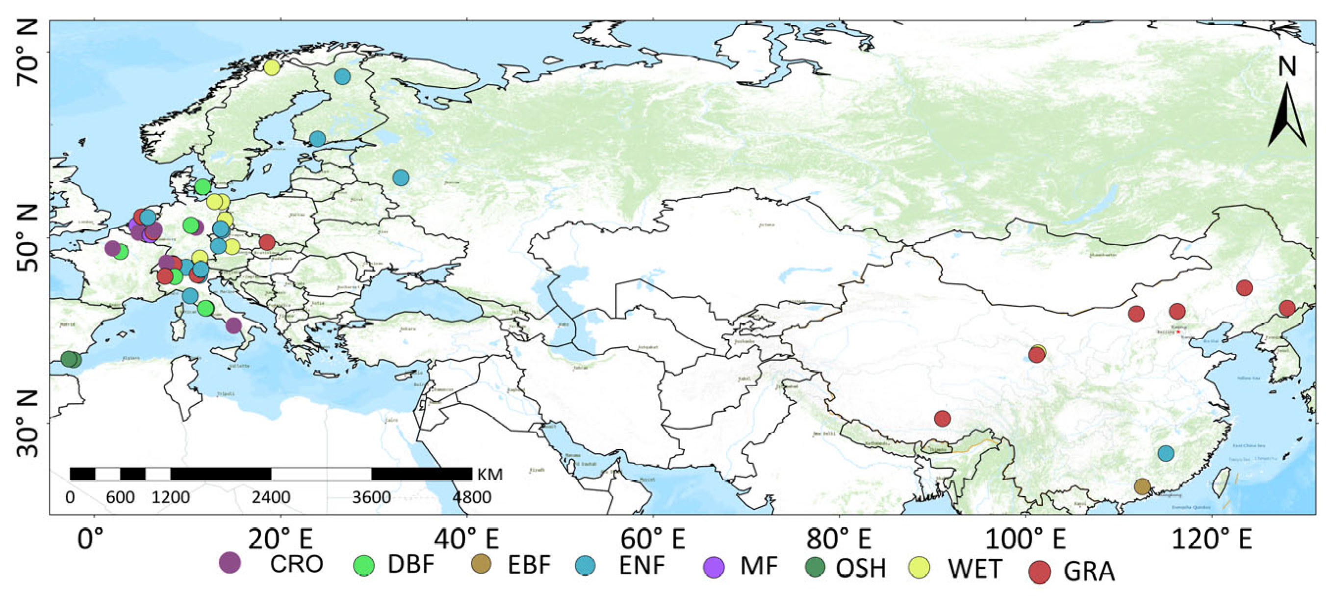The data were sourced from the Fluxnet website (http://fluxnet.fluxdata.org/, accessed on 1 February 2024). The flux stations selected in this study covered eight different types of subsurfaces, including croplands (CRO), deciduous broadleaf forest (DBF), evergreen broadleaf forest (EBF), evergreen needleleaf forest (ENF), mixed forest (MF), open shrublands (OSH), wetlands (WET), and grasslands (GRA) (Figure 1). The data selected for this study covered all valid time periods in China, while the time period selected for Europe was from 2010 to 2014.

2.2. MODIS Data

The aerosol optical depth (AOD) data from the moderate-resolution imaging spectroradiometer (MODIS), selected for this study, is a Level 2 product released by NASA (https://ladsweb.modaps.eosdis.nasa.gov/search/, accessed on 1 February 2024). This dataset can be used to obtain atmospheric aerosol optical properties (e.g., optical and size distributions) and mass concentrations for the global marine and terrestrial environments. The MODIS AOD products have a spatial resolution of 3 km and a data format of HDF4 and contain two products, MOD04_3K and MYD04_3K [26]. In this study, we downloaded MOD AOD and MYD AOD data for Eurasia from 2002 to 2020 and then extracted a dataset with the optical depth parameter “Optical_Depth_Land_And_Ocean” for terrestrial aerosols in the 550 nm band. We used the maximum value method to maximally synthesize two AOD data products for the same day to obtain one image per day.

The LAI data were selected from the MOD15A2H dataset (https://ladsweb.modaps.eosdis.nasa.gov/search/order/1/MOD15A2H--61, accessed on 1 February 2024). The dataset has a spatial resolution of 500 m and a temporal resolution of 8 days. We set each day of the 8-day cycle to the same value to match the meteorology and AOD. The AOD and LAI datasets were preprocessed using the MCTK (MODIS Conversion Toolkit) plug-in and the ENVI/IDL (The Environment for Visualizing Images/Interface Description Language) language, such as batch reprojection, clipping, and extraction. The extracted AOD and LAI were matched with FLUXNET2015 data and used as one of the variables for retrieving H and LE.

The land cover data used in the study are derived from the MCD12Q1 dataset. This dataset includes 17 major land cover types classified according to the International Geosphere-Biosphere Programme (IGBP). These types consist of 11 natural vegetation types, 3 land development and mixed land classes, and 3 non-vegetated land types. MCD12Q1 is an annual global 500-m land cover type product generated by the MODIS Terra + Aqua satellites. It employs five different land cover classification schemes and utilizes techniques such as supervised decision tree classification for information extraction. For this research, the first land cover classification scheme, namely the global vegetation classification scheme by IGBP, was utilized. The dataset can be accessed and obtained for free through the website https://ladsweb.modaps.eosdis.nasa.gov/search/, accessed on 1 February 2024.

2.3. ERA5 Atmospheric Reanalysis Data

The ERA5 data, which is the latest high-resolution reanalysis data, has been released by the European Centre for Medium-Range Weather Forecasts (ECMWF). The dataset provides hourly estimates of atmospheric, terrestrial, and oceanic climate variables at a spatial resolution of 0.25° [27,28,29]. ERA5 is the fifth generation of atmospheric reanalysis products. In this study, ERA5 data were used to drive a deep neural network model trained to retrieve surface latent heat and sensible heat flux on a regional scale. Daily values of six climate reanalysis parameters were selected for the study, including 2 m air temperature, 2 m dew point temperature, total precipitation, top net solar radiation, 10 m u-wind component, and 10 m v-wind component. The daily minimum and maximum air temperatures at 2 m were derived from the hourly 2 m air temperature data. Dew point temperature data was used to calculate relative humidity. We downloaded data for four time periods (00.00, 06.00, 12.00, and 18.00 h) from 2010–2020 and pre-processed the data with single-band extraction and cropping using ARCGIS 10.2 software. The data for the four time periods were averaged to obtain daily data. MODIS AOD and MODIS LAI data were resampled to have the same spatial resolution as the ERA5 data.

2.4. FLUXCOM Products

In this research, monthly product data corresponding to a spatial resolution of 5° and a temporal resolution aligned with the validation site intervals were downloaded to validate the regional retrieval of H and LE. The FLUXCOM Remote Sensing (RS) dataset is a component of the FLUXCOM product used for global surface flux estimation. In the RS configuration, nine machine learning methods were employed to generate grid products with a temporal resolution of 8 days and a spatial resolution of 0.0833° for the period from 2001 to 2015 [30]. This dataset utilizes satellite remote sensing technology to retrieve surface flux information and provides more comprehensive observational data. It includes various remote sensing data sources such as MODIS and GRACE, which are used to obtain observational data on surface radiation, temperature, humidity, gases, and water vapor fluxes. By utilizing these remote sensing data, the FLUXCOM RS dataset can offer more comprehensive and accurate observations of surface fluxes, revealing the processes of energy, water, and carbon cycles in terrestrial ecosystems. The FLUXCOM RS dataset was utilized to validate and monitor the inversion results of surface water and heat fluxes in climate models. These data can be obtained free of charge through the Energy Flux–FLUXCOM website.

3. Methods

3.1. Energy Balance Closure Correction and Evaluation

The energy closure correction and evaluation methods for evaluating and correcting the energy closure of latent heat flux and sensible heat flux are as follows. According to the first law of thermodynamics, the surface energy balance is expressed as follows [14]:

$$LE+H=R_n-G-S-Q$$

(1)

According to Equation (1), $R_n$ is the net radiation, G is the soil heat flux, S is the canopy heat storage, and Q is the total additional energy. Generally, the value of Q is very small and can be neglected.

In ecosystems with low vegetation, such as bare ground, the values of S and Q are typically small. Therefore, the energy balance equation can be simplified to:

$$LE+H=R_n-G$$

(2)

When the turbulent energy (LE + H) and the surface effective energy ($R_n-G$) are the same, this is energy closure; otherwise, the energy is not closed. The energy balance ratio (EBR) used in this study is used to assess the energy closure:

$$EBR=\frac{{\displaystyle \sum (LE+H)}}{{\displaystyle \sum (R_n-G)}}$$

(3)

3.2. Relative Humidity (RH) Calculation

Relative humidity was calculated using the vapor pressure deficit from the flux tower dataset using Equation (4):

$$RH=1-\frac{VPD}{e_{sat}}$$

(4)

In Equation (4), $e_{sat}$ is the saturated water vapor pressure calculated from the Clausius–Clapeyron relation and the average daily temperature. The formula is:

$$e_{sat}(T)=e_{s0}\exp (\frac{L_v}{R_v}[\frac{1}{T_0}-\frac{1}{T}])$$

(5)

In Equation (5), $T_0$ and $e_{s0}$ are integral constants with values of 273.26 K and 611 Pa, respectively; $L_v$ is the latent heat of evaporation (2.5 × 106 J/kg), and $R_v$ is the specific gas constant for water vapor.

3.3. Artifificial Neural Network Model Training

There are complex nonlinear relationships between various variables and surface fluxes. This study aims to use deep learning artificial neural networks to model H and LE, as this method has a strong nonlinear capability. Different factors have varying impacts on the changes in surface fluxes. Meteorological factors such as temperature, humidity, wind speed, and radiation are important in regulating or influencing the water and energy exchange processes. For example, temperature is a key factor in affecting evaporation, wind speed affects the diffusion of atmospheric moisture, and solar radiation is the input energy to the Earth’s surface. Aerosols also have complex impacts on surface fluxes. They regulate heat transfer and humidity adjustment during the surface energy exchange process by absorbing and scattering solar radiation, influencing atmospheric temperature, promoting cloud formation, etc. Changes in vegetation coverage directly affect the albedo, LE, and H, thus having significant impacts on the climate system. This study employed LAI and vegetation types as indicators to represent and capture the vegetation change effect.

Table 1. Variables entered into the neural network model.

Variables	Field	Units	Data Sources	Purpose
Top-of-atmosphere shortwave radiation	SW_IN_POT	W/m2	The daily integrated dataset	Input variables
Average temperatures	Tmean	°C	Half hour or hour dataset	Input variables
Maximum temperature	Tmax	°C	Half hour or hour dataset	Input variables
Minimum temperature	Tmin	°C	The daily integrated dataset	Input variables
Vapor pressure deficit	VPD	hpa	The daily integrated dataset	VPD is used to calculate RH
Average wind speed	WS	m/s	The daily integrated dataset	Input variables
Aerosol optical depth	AOD		MOD04_3K and MYD04_3K	Input variables
Leaf area index	LAI		MOD15A2H	Input variables
Land cover type	LC_Type1		MCD12Q1	Input variables
Latent heat flux	LE	W/m2	The daily integrated dataset	Output variables
Sensible heat flux	H	W/m2	The daily integrated dataset	Output variables

details the model input variables selected for this study.

We sorted the Fluxnet2015 data according to chronological order so that the different variables corresponded to each other. After data preprocessing, we divide the data into different datasets for training, validation, and testing. During the training phase of the ANN model, the datasets were randomly divided into training, validation, and testing datasets, comprising 80%, 10%, and 10% of the data, respectively. Including some missing records, the training, validation, and testing datasets include 6372, 655, and 655 daily-scale sample data, respectively. In the model training phase, in order to control the data quality and improve the predictive ability of the model, the data selected for this study are measured data (labeled as 0) and vacancy-filled data with good assessment quality (labeled 1). Data with an interpolation quality less than 1 were not involved in model training. The study removes the missing data of the day in order to reduce the invalid and redundant input information during the training of the ANN model, thus reducing the training time of the model. Generally, the more information about variables inputted into a model, the better its predictive capability. However, it is also necessary to consider the complexity and generalization ability of the model. The more input variables, the stronger the extrapolation ability of the model. Therefore, the optimal combination of input variables is selected while considering the extrapolation capability of the model. Wang et al. [20] experimentally obtained the optimal combination of variables input to the ANN model and retrieved the global surface latent heat and sensible heat flux. This study used a simple model structure (2 hidden layers with 14 neurons per layer) based on the optimal model from previous experiments [20]. The model training was performed through several experiments to obtain a stable network model, and the model was tested using Pearson’s correlation coefficient (R) and root mean square error (RMSE) as evaluation metrics.

4. Results

4.1. Accuracy Verification for an Overall Sample

In this study, we developed four models to retrieve latent heat flux (LE) and sensible heat flux (H). Each model considered different factors: The first model considered meteorological factors, the second model considered meteorological factors and aerosols, the third model considered meteorological factors and vegetation variations (including LAI and vegetation type), and the fourth model integrated meteorological factors, aerosols, and vegetation variations. The results showed that, among the overall samples, the model considering only meteorological factors had the largest prediction errors for latent heat and sensible heat flux (R_H = 0.70, RMSE_H = 34.01; R_LE = 0.74, RMSE_LE = 31.01; Figure 2). The model that comprehensively considered meteorological factors, aerosols, and vegetation variations exhibited the highest correlation with observed values of latent heat and sensible heat flux at the monitoring sites and had the smallest errors (R_H = 0.85, RMSE_H = 24.88; R_LE = 0.88, RMSE_LE = 22.25).

4.2. Verification at Different Vegetation Cover Types

In addition to validating the entire sample, the study validated different ecosystems using the four models with the aim of assessing the ability of the four groups of models to retrieve H and LE under different vegetation cover types. Five major ecosystem types were selected for this study, including CRO, DBF, ENF, GRA, and WET. It was found that the four groups of models had different predictive abilities for surface latent heat and sensible heat flux in different ecosystems.

Based on the retrieval results of H (Figure 3a,c), there are relatively significant differences in the retrieval results obtained by the four models for the GRA and WET types. However, the differences in H retrieval among the four models are relatively small for the CRO, DBF, and ENF vegetation types. As for the retrieval results of LE (Figure 3b,d), the differences in results obtained by the four models are minimal for the ENF vegetation type, while there are significant differences in retrieval capability among the four models for the other four vegetation types. Overall, considering meteorological factors and vegetation changes, as well as a comprehensive consideration of meteorological factors, aerosols, and vegetation changes, these two model approaches show better retrieval performance for LE.

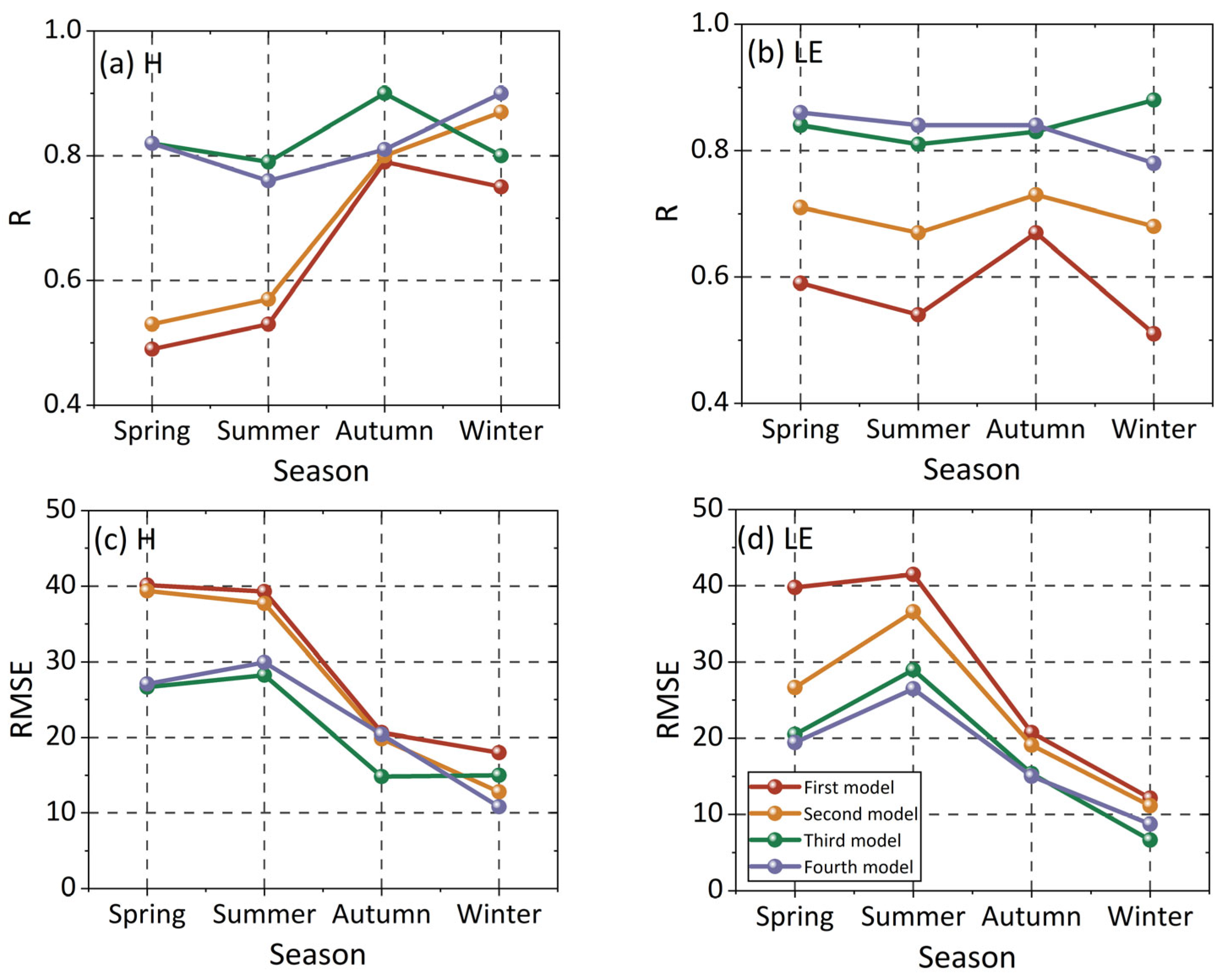
4.3. Model Validation for Seasons

The four models showed different abilities to retrieve LE and H in different seasons (Figure 4). Overall, during the spring and summer seasons, the four model groups show significant differences in predicting H and LE. Models that consider meteorological factors and vegetation changes, as well as those that comprehensively incorporate meteorological factors, aerosols, and vegetation changes, demonstrate better retrieval performance for H and LE. Models that solely consider meteorological factors exhibit larger errors and lower correlations in predicting H and LE values.

4.4. Case Studies and Validation of Results for Large-Scale Surface Water and Heat Fluxes Retrieval

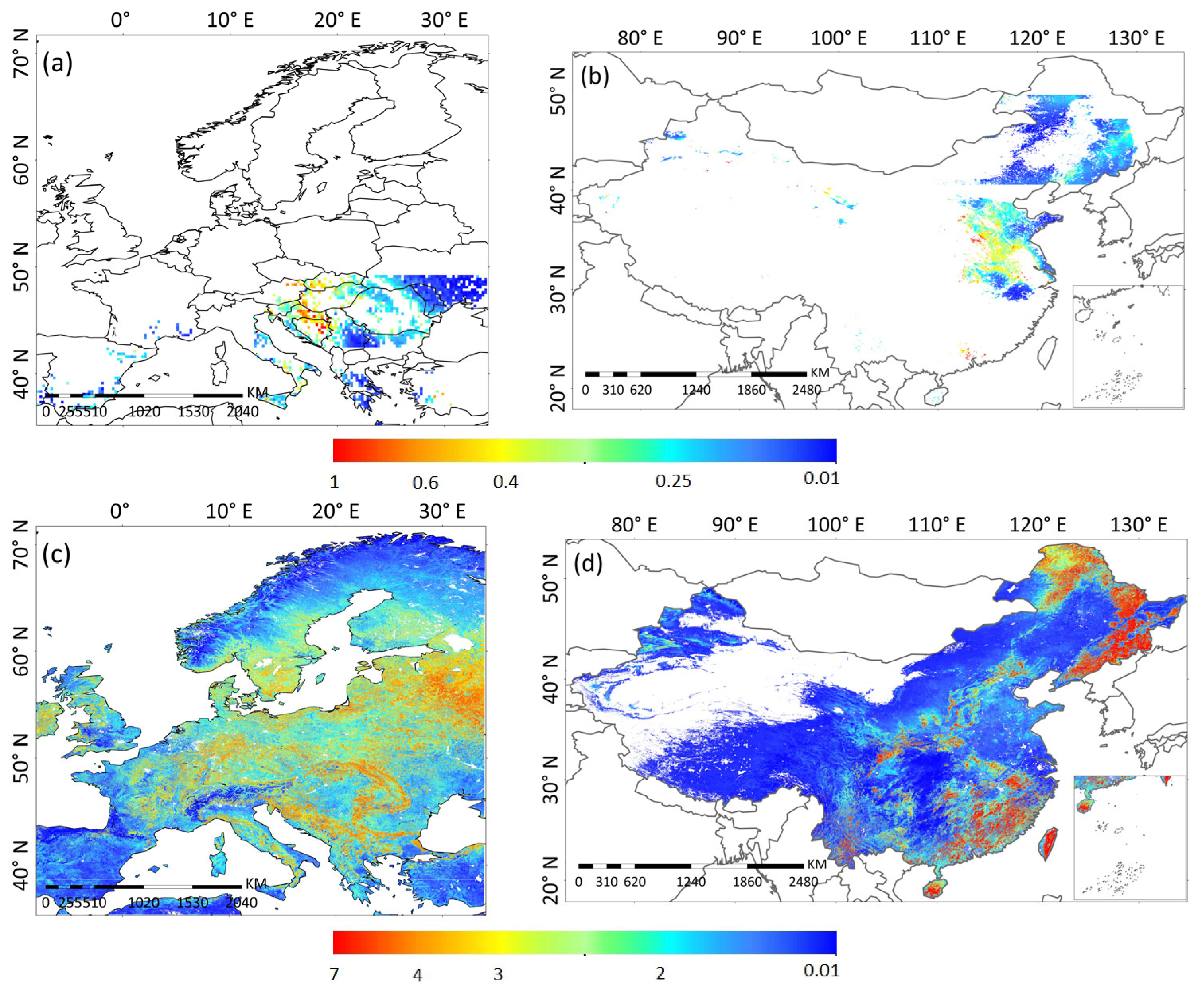
In this study, four pre-trained mature deep neural network models driven by ERA5 data were used to retrieve H and LE in China and Europe from 2010 to 2020. The study shows the spatial distribution of AOD and LAI in China and Europe on 1 June 2018 (Figure 5). Aerosols over Europe on that day were mainly distributed in the southern region. There were sporadic aerosol distributions in northwest China, and aerosols were mainly distributed in northeast and east China. The LAI in Europe was relatively high in the central region. The LAI in China is relatively high in the northeastern, central, and eastern regions.

Figure 6 displays the spatial distribution of H and LE retrieved by four models in Europe on 1 June 2018. The retrieval results for H indicate that when aerosols are present in the atmosphere, the second model shows higher H values at the corresponding locations (Figure 6b). Compared to the first three models, the fourth model retrieves lower H values in the central and southern regions. In Norway, the third and fourth models retrieve lower H values compared to the first and second models. The fourth model is capable of presenting more refined retrieval results (Figure 6d). The retrieval results for LE suggest that when aerosols are present in the atmosphere, the second model shows lower LE values at the corresponding locations (Figure 6f). Compared to the first two models, the third and fourth models exhibit more refined retrieval results. In the western and central regions of Europe, the third and fourth models (Figure 6g,h) retrieve lower LE values compared to the first and second models. Figure 7 shows the spatial distribution of H and LE retrieved by four models in China on 1 June 2018. Overall, in the eastern and central regions of China, the values of H and LE retrieved by the first and second models are higher than those retrieved by the third and fourth models. Similarly, when vegetation changes are considered in the third and fourth models, they can retrieve H and LE with relatively refined results.

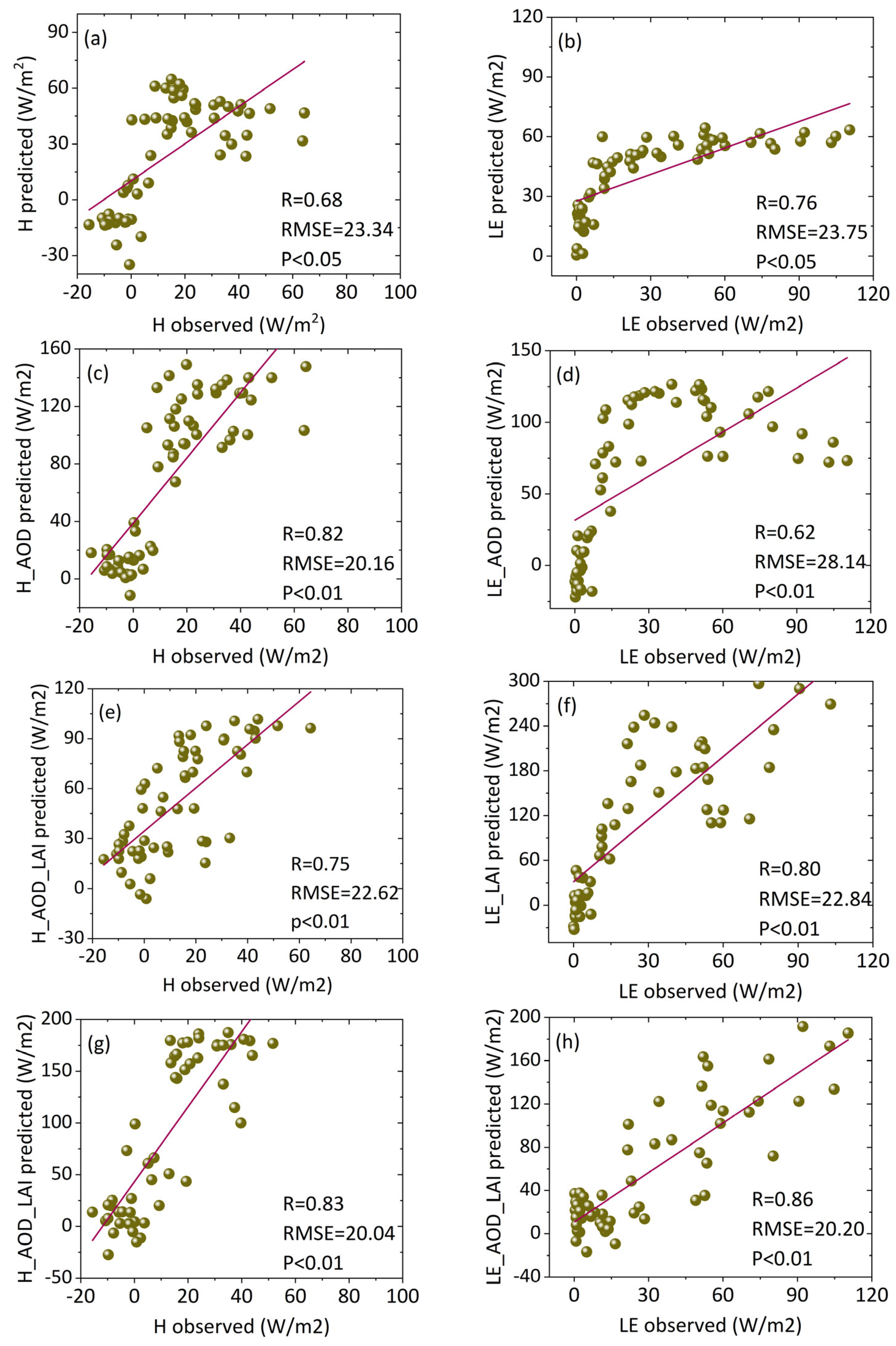
In order to validate the reliability of the retrieval results, we randomly selected a site (FLX_DE-Geb, 2010–2014) in this study. It was required that the site have valid data from 2010 to 2020 and not participate in model construction. Using the monthly scatter plot of this site (Figure 8), we validated the data retrieved from four models. Overall, we found that the model retrieval combining meteorological factors, aerosols, and vegetation changes had the best correlation and the smallest error in comparison to the observation site for both H and LE (R_H = 0.83, RMSE_H = 20.04; R_LE = 0.86, RMSE_LE = 20.20; Figure 8g,h). The error of H retrieved by the model considering meteorological factors and aerosols was only second to the fourth model (R_H = 0.82, RMSE_H = 20.16; Figure 8c). Similarly, the error of LE retrieved by the model considering meteorological factors and vegetation changes was also only second to the fourth model (R_LE = 0.80, RMSE_LE = 22.84; Figure 8f).

Furthermore, we conducted verification of the retrieval results of the four sets of models with FLUXCOM products at corresponding locations (Figure 9). It can be observed that the retrieval of H by the second and fourth sets of models is highly correlated with FLUXCOM products. The correlation between the retrieval of LE by the fourth set of models and FLUXCOM products is better compared to the other three models. Therefore, considering meteorological factors, aerosol, and vegetation changes, the overall retrieval performance of the model is better (R_H = 0.93, RMSE_H = 27.10; R_LE = 0.87, RMSE_LE = 24.38). This also indicates the need to comprehensively consider the impact of aerosol and vegetation changes on retrieving H and LE.

5. Discussion

For the second model, there are some regions where aerosols are not present in the air, but the model input still contains meteorological data. These data can be used as inputs for machine learning models to estimate the corresponding latent heat flux and sensible heat flux under the given conditions. Machine learning has strong nonlinear capabilities. After analyzing the H and LE in China and Europe, we found that the spatial distribution trends of LE and H obtained by the four models are not completely consistent. Aerosol particles can directly absorb or scatter solar shortwave radiation and indirectly affect solar shortwave radiation and terrestrial longwave radiation by changing or influencing cloud characteristics. If aerosols are not considered when retrieving H and LE, retrieval errors will occur when aerosols exist in the atmosphere. Vegetation changes can affect transpiration and, thus, the partitioning of surface energy fluxes. Generally, an increase in vegetation coverage leads to an enhanced transpiration, whereas decreased vegetation coverage reduces transpiration, resulting in a decrease in LE and an increase in H [31]. Higher vegetation coverage can increase soil moisture and enhance water storage capacity, resulting in improved water utilization and reduced runoff loss, thereby regulating surface water and heat fluxes. Conversely, when vegetation coverage decreases, both soil moisture and water storage capacity decrease. These factors combined have an impact on surface fluxes and subsequently influence energy exchange and water cycling processes. Therefore, considering vegetation changes is crucial in the retrieval of surface water and heat fluxes.

The availability of sufficient flux tower observatories has a significant impact on the retrieval results. In this study, the number of flux tower observatories in Europe is relatively high, and their distribution is relatively centralized. In contrast, the number of flux tower observatories in China is relatively small, and their distribution is relatively decentralized, resulting in larger errors in the retrieval results. Deep neural network models, being more adaptable to large amounts of sample data, enable more accurate simulations.

6. Conclusions

In this study, we constructed four sets of machine learning models for retrieving H and LE based on meteorological factors, aerosol, and vegetation changes. The first set of models considered meteorological factors, the second set considered meteorological factors and aerosol, the third set considered meteorological factors and vegetation changes, and the fourth set comprehensively considered meteorological factors, aerosols, and vegetation changes. We compared the retrieval capabilities of these four models. The ERA5 reanalysis, AOD, LAI, and vegetation type data were used to drive these four models and to retrieve H and LE within our study region. The results were then validated by comparing them with site data that were not involved in model construction, as well as with the FLUXCOM product. The findings are summarized as follows:

(1) The model, integrating meteorological factors, aerosols, and vegetation changes, has superior retrieval performance in the retrieval of surface water and heat fluxes of whole samples. Among different vegetation types, the four models exhibited relatively larger discrepancies in retrieving H for GRA and WET types, while the discrepancies in retrieving H for CRO, DBF, and ENF vegetation types were comparatively smaller. Regarding LE retrieval, the four models displayed the fewest differences in retrieval under the ENF vegetation type, whereas significant differences existed in the capability to retrieve LE for the other four vegetation types. From a seasonal perspective, the models considering meteorological factors and vegetation changes, as well as the models comprehensively considering meteorological factors, aerosols, and vegetation changes, performed well in retrieving surface fluxes.

(2) The results suggested that the spatial distribution of H and LE obtained by the four deep neural network models was not completely consistent. When aerosols were present in the atmosphere over China and Europe, the model considering both meteorological factors and aerosols retrieved higher values of H and lower values of LE as compared to the model considering only meteorological factors at corresponding locations. The model considering meteorological factors and vegetation variations, as well as the model considering a comprehensive combination of meteorological factors, aerosols, and vegetation variations, retrieved lower values of H and LE in most regions as compared to the other two models.

(3) Through validation with observation stations that were not involved in model construction, we found that the model considering meteorological factors, aerosols, and vegetation variations had the best correlation and smallest error in retrieving H and LE. By comparison with FLUXCOM products, it was found that the retrieved H and LE were more accurate in general by considering meteorological factors, aerosols, and vegetation changes. Therefore, considering the effects of aerosols and vegetation changes, the retrieval accuracy of surface fluxes can be significantly improved. The methods and optimized model provided in this study can be used to retrieve or predict long-term and large-scale dynamic surface fluxes in the future.

References

- Chen, J.; Dong, G.; Chen, J.; Jiang, S.; Qu, L.; Legesse, T.G.; Zhao, F.; Tong, Q.; Shao, C.; Han, X. Energy balance and partitioning over grasslands on the Mongolian Plateau. Ecol. Indic. 2022, 135, 108560. [Google Scholar] [CrossRef]
- Chen, L.; Chen, H.; Wang, R.; Wei, G. Analysis of Spatiotemporal Distribution of Evaporation Fractions of Different Vegetation Types Based on FLUXNET Site. IEEE Geosci. Remote Sens. Lett. 2024, 21, 1000605. [Google Scholar] [CrossRef]
- Qiu, L.; Wu, Y.; Yu, M.; Shi, Z.; Yin, X.; Song, Y.; Sun, K. Contributions of vegetation restoration and climate change to spatiotemporal variation in the energy budget in the loess plateau of China. Ecol. Indic. 2021, 127, 107780. [Google Scholar] [CrossRef]
- Feigenwinter, C.; Vogt, R.; Parlow, E.; Lindberg, F.; Marconcini, M.; Del Frate, F.; Chrysoulakis, N. Spatial Distribution of Sensible and Latent Heat Flux in the City of Basel (Switzerland). IEEE J. Sel. Top. Appl. Earth Obs. Remote. Sens. 2018, 11, 2717–2723. [Google Scholar] [CrossRef]
- Mazhar, U.; Jin, S.; Hu, T.; Bilal, M.; Ali, A.; Atique, L. Long-Time Variation and Mechanism of Surface Energy Budget Over Diverse Geographical Regions in Pakistan. IEEE J. Sel. Top. Appl. Earth Obs. Remote. Sens. 2022, 15, 5203–5213. [Google Scholar] [CrossRef]
- Yang, K.; Qin, J.; Guo, X.; Zhou, D.; Ma, Y. Method development for estimating sensible heat flux over the Tibetan Plateau from CMA data. J. Appl. Meteorol. Clim. 2009, 48, 2474–2486. [Google Scholar] [CrossRef]
- Anderson, R.G.; Canadell, J.G.; Randerson, J.T.; Jackson, R.B.; Hungate, A.B.; Baldocchi, D.D.; Ban-Weiss, A.G.; Bonan, G.B.; Caldeira, K.; Cao, L.; et al. Biophysical considerations in forestry for climate protection. Front. Ecol. Environ. 2010, 9, 174–182. [Google Scholar] [CrossRef]
- Lin, H.; Li, Y.; Zhao, L. Partitioning of sensible and latent heat fluxes in different vegetation types and their spatiotemporal variations based on 203 FLUXNET sites. J. Geophys. Res. Atmos. 2022, 127, e2022JD037142. [Google Scholar] [CrossRef]
- Li, Y.; Zhao, M.; Motesharrei, S.; Mu, Q.; Kalnay, E.; Li, S. Local cooling and warming effects of forests based on satellite observations. Nat. Commun. 2015, 6, 6603. [Google Scholar] [CrossRef] [PubMed]
- Houspanossian, J.; Nosetto, M.; Jobbágy, E.G. Radiation budget changes with dry forest clearing in temperate Argentina. Glob. Change Biol. 2013, 19, 1211–1222. [Google Scholar] [CrossRef] [PubMed]
- Wang, S.; Ma, Y.; Liu, Y. Simulation of sensible and latent heat fluxes on the Tibetan Plateau from 1981 to 2018. Atmos. Res. 2022, 271, 106129. [Google Scholar] [CrossRef]
- Zhang, M.; Wang, J.; Li, S. Tempo-spatial changes and main anthropogenic influence factors of vegetation fractional coverage in a large-scale opencast coal mine area from 1992 to 2015. J. Clean. Prod. 2019, 232, 940–952. [Google Scholar] [CrossRef]
- Wei, J.; Lu, B.; Song, Y.; Chen, H.; Weng, Z. Anthropogenic aerosols weaken land–atmosphere coupling over North China. Geophys. Res. Lett. 2023, 50, e2023GL105685. [Google Scholar] [CrossRef]
- Wang, R.; Gentine, P.; Yin, J.; Chen, L.; Chen, J.; Li, L. Long-term relative decline in evapotranspiration with increasing runoff on fractional land surfaces. Hydrol. Earth Syst. Sci. 2021, 25, 3805–3818. [Google Scholar] [CrossRef]
- Jung, M.; Reichstein, M.; Ciais, P.; Seneviratne, S.I.; Sheffield, J.; Goulden, M.L.; Bonan, G.; Cescatti, A.; Chen, J.; De Jeu, R.; et al. Recent decline in the global land evapotranspiration trend due to limited moisture supply. Nature 2010, 467, 951–954. [Google Scholar] [CrossRef] [PubMed]
- Jung, M.; Reichstein, M.; Bondean, A. Towards global empirical upscaling of FLUXNET eddy covariance observations: Validation of a model tree ensemble approach using a biosphere model. Biogeosciences 2009, 6, 2001–2013. [Google Scholar] [CrossRef]
- Alemohammad, S.H.; Fang, B.; Konings, A.G.; Aires, F.; Green, J.K.; Kolassa, J.; Miralles, D.; Prigent, C.; Gentine, P. Water, Energy, and Carbon with Artificial Neural Networks (WECANN): A statistically-based estimate of global surface turbulent fluxes and gross primary productivity using solar-induced fluorescence. Biogeosciences 2017, 14, 4101–4124. [Google Scholar] [CrossRef]
- Li, Z.; Guo, J.; Ding, A.; Liao, H.; Liu, J.; Sun, Y.; Wang, T.; Xue, H.; Zhang, H.; Zhu, B. Aerosol and boundary-layer interactions and impact on air quality. Natl. Sci. Rev. 2017, 4, 810–833. [Google Scholar] [CrossRef]
- Jung, M.; Reichstein, M.; Margolis, H.A.; Cescatti, A.; Richardson, A.D.; Arain, M.A.; Arneth, A.; Bernhofer, C.; Bonal, D.; Chen, J.; et al. Global patterns of land-atmosphere fluxes of carbon dioxide, latent heat, and sensible heat derived from eddy covariance, satellite, and meteorological observations. J. Geophys. Res. Atmos. 2011, 116, G00J07. [Google Scholar] [CrossRef]
- Decker, M.; Brunke, M.; Wang, Z.; Sakaguchi, K.; Zeng, X.; Bosilovich, M. Evaluation of the reanalysis products from gsfc, ncep, and ecmwf using flux tower observations. J. Climate. 2012, 6, 25. [Google Scholar] [CrossRef]
- Li, F.; Kustas, W.P.; Anderson, M.C.; Prueger, J.H.; Scott, R.L. Effect of remote sensing spatial resolution on interpreting tower-based flux observations. Remote Sens. Environ. 2008, 112, 337–349. [Google Scholar] [CrossRef]
- Bai, P. Comparison of remote sensing evapotranspiration models: Consistency, merits, and pitfalls. J. Hydrol. 2023, 617, 128856. [Google Scholar] [CrossRef]
- Mazrooei, A.; Reitz, M.; Wang, D.; Sankarasubramanian, A. Urbanization impacts on evapotranspiration across various spatio-temporal scales. Earth’s Future 2021, 9, e2021EF002045. [Google Scholar] [CrossRef]
- Mu, Q.Z.; Zhao, M.S.; Running, S.W. Improvements to a MODIS global terrestrial evapotranspiration algorithm. Remote Sens. Environ. 2011, 115, 1781–1800. [Google Scholar] [CrossRef]
- Zheng, C.; Li, J.; Hu, G. Global land surface evapotranspiration monitoring by ETMonitor model driven by multi-source satellite earth observations. J. Hydrol. 2022, 613 Pt B, 128444. [Google Scholar] [CrossRef]
- Chen, L.; Wang, R.; Han, J.; Zha, Y. Influence of observation angle change on satellite retrieval of aerosol optical depth. Tellus Ser. B Chem. Phys. Meteorol. B 2021, 73, 1–14. [Google Scholar] [CrossRef]
- Liu, L.; Gu, H.; Xie, J.; Xu, Y.P. How well do the ERA-Interim, ERA-5, GLDAS-2.1 and NCEP-R2 reanalysis datasets represent daily air temperature over the Tibetan Plateau? Int. J. Climatol. 2020, 41, 1484–1505. [Google Scholar] [CrossRef]
- Zou, J.; Lu, N.; Jiang, H.; Qin, J.; Yao, L.; Xin, Y.; Su, F. Performance of air temperature from ERA5-Land reanalysis in coastal urban agglomeration of Southeast China. Sci. Total Environ. 2022, 828, 154459. [Google Scholar] [CrossRef]
- Zajicek, R. Climatology and Long-Term Trends in the Stratospheric Temperature and Wind Using ERA5. Remote Sens. 2021, 13, 4923. [Google Scholar]
- Jung, M.; Koirala, S.; Weber, U.; Ichii, K.; Gans, F.; Camps-Valls, G.; Papale, D.; Schwalm, C.; Tramontana, G.; Reichstein, M. The FLUXCOM ensemble of global land-atmosphere energy fluxes. Sci. Data 2019, 6, 74. [Google Scholar] [CrossRef]
- Duveiller, G.; Hooker, J.; Cescatti, A. The mark of vegetation change on Earth’s surface energy balance. Nat. Commun. 2018, 9, 679. [Google Scholar] [CrossRef] [PubMed]
Figure 1.
Spatial distribution of flux tower observation stations selected in the study.
Figure 2.
Scatter density diagram of ANN model validation at daily scale (a,b) represent the first model considering only meteorological factors; (c,d) represent the second model considering meteorological factors and aerosols; (e,f) represent the third model considering meteorological factors and vegetation variation; (g,h) represent the fourth model comprehensively considering meteorological factors, aerosols, and vegetation variation. Number of sample points 6372. The black solid line is the best linear fit line and the grey dashed line is the 1:1 fit line.
Figure 3.
R and RMSE of four models under different vegetation type covers. (a) Correlation of H predicted by the four models with observed data. (b) Correlation of LE predicted by the four models with observed data. (c) Errors between H predicted by the four models and the observed data. (d) Errors between LE predicted by the four models and the observed data. (The first model only considers meteorological factors; the second model considers both meteorological factors and aerosols; the third model considers the changes in meteorological factors and vegetation; and the fourth model comprehensively considers meteorological factors, aerosols, and vegetation changes).
Figure 4.
R and RMSE for the four models in different seasons. (a) Correlation of H predicted by the four models with observed data. (b) Correlation of LE predicted by the four models with observed data. (c) Errors between H predicted by the four models and the observed data. (d) Errors between LE predicted by the four models and the observed data.
Figure 5.
Spatial distribution of AOD and LAI in China and Europe on 1 June 2018 ((a,b) show the spatial distribution of AOD, (c,d) show the spatial distribution of LAI).
Figure 6.
Spatial distribution of H and LE for the four model retrievals on 1 June 2018 in parts of Europe. ((a–d) are the H values retrieved by the first to fourth models. (e–h) are the LE retrieved by the first to the fourth models. The first model considers only meteorological factors. The second model considers meteorological factors and aerosols. The third model considers meteorological factors and vegetation changes, and the fourth model combines meteorological factors, aerosols, and vegetation changes).
Figure 7.
Spatial distribution of H and LE for four model retrievals on 1 June 2018 in China. ((a–d) are the first to fourth model retrieved H. (e–h) are the first to fourth model retrieved LE).
Figure 8.
Validation results for H and LE at regional scales (The first model: (a,b) considering only meteorological factors. The second model: (c,d) considering meteorological factors and aerosols. The third model: (e,f) considering meteorological factors and vegetation changes. The verification results of (g,h) are comprehensive considerations of three factors: meteorological factors, aerosols, and vegetation changes). The solid red line is the line of best linear fit.
Figure 9.
The validation results of the four sets of models and FLUXCOM product at the corresponding location of this site are as follows.(The first model: (a,b) considering only meteorological factors. The second model: (c,d) considering meteorological factors and aerosols. The third model: (e,f) considering meteorological factors and vegetation changes. The verification results of (g,h) are comprehensive considerations of three factors: meteorological factors, aerosols, and vegetation changes). The solid red line is the line of best linear fit.