
Pre-Processing of Simulated Synthetic Aperture Radar Image Scenes Using Polarimetric Enhancement for Improved Ship Wake Detection


Abstract
1. Introduction
2. Background
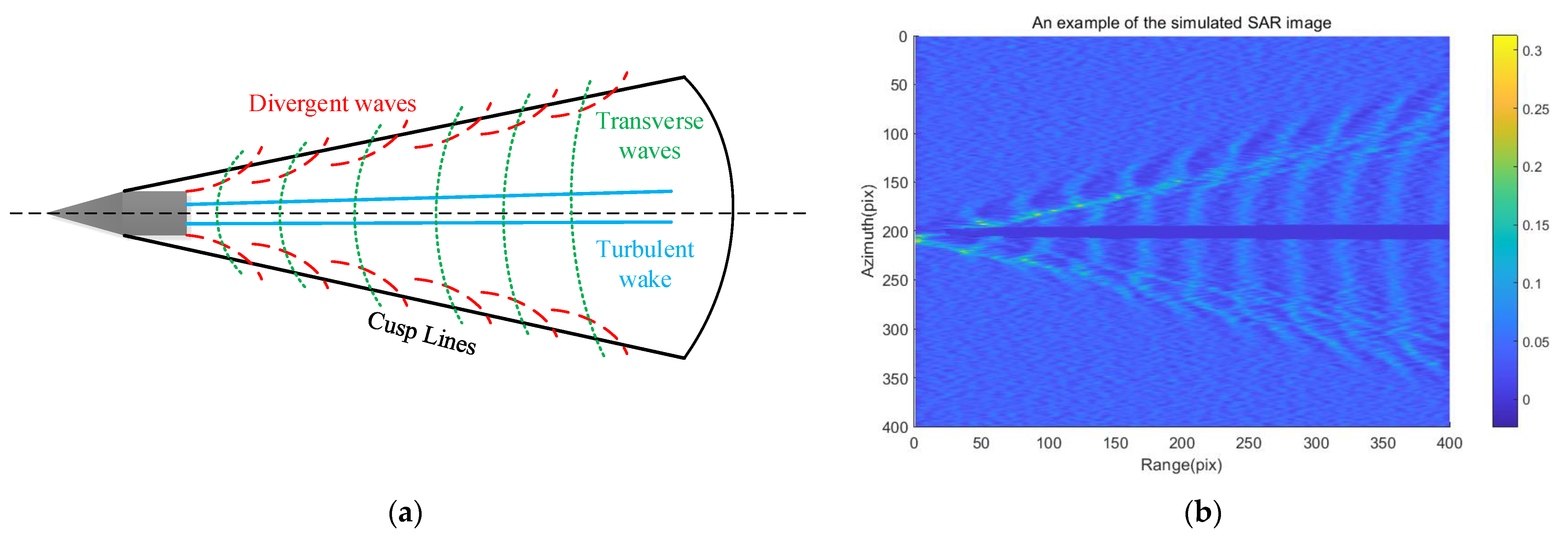
2.1. Ship Wake Simulation in SAR Images
2.2. PWF and PDOF Filter
2.2.1. PWF Filter
2.2.2. PDOF Filter
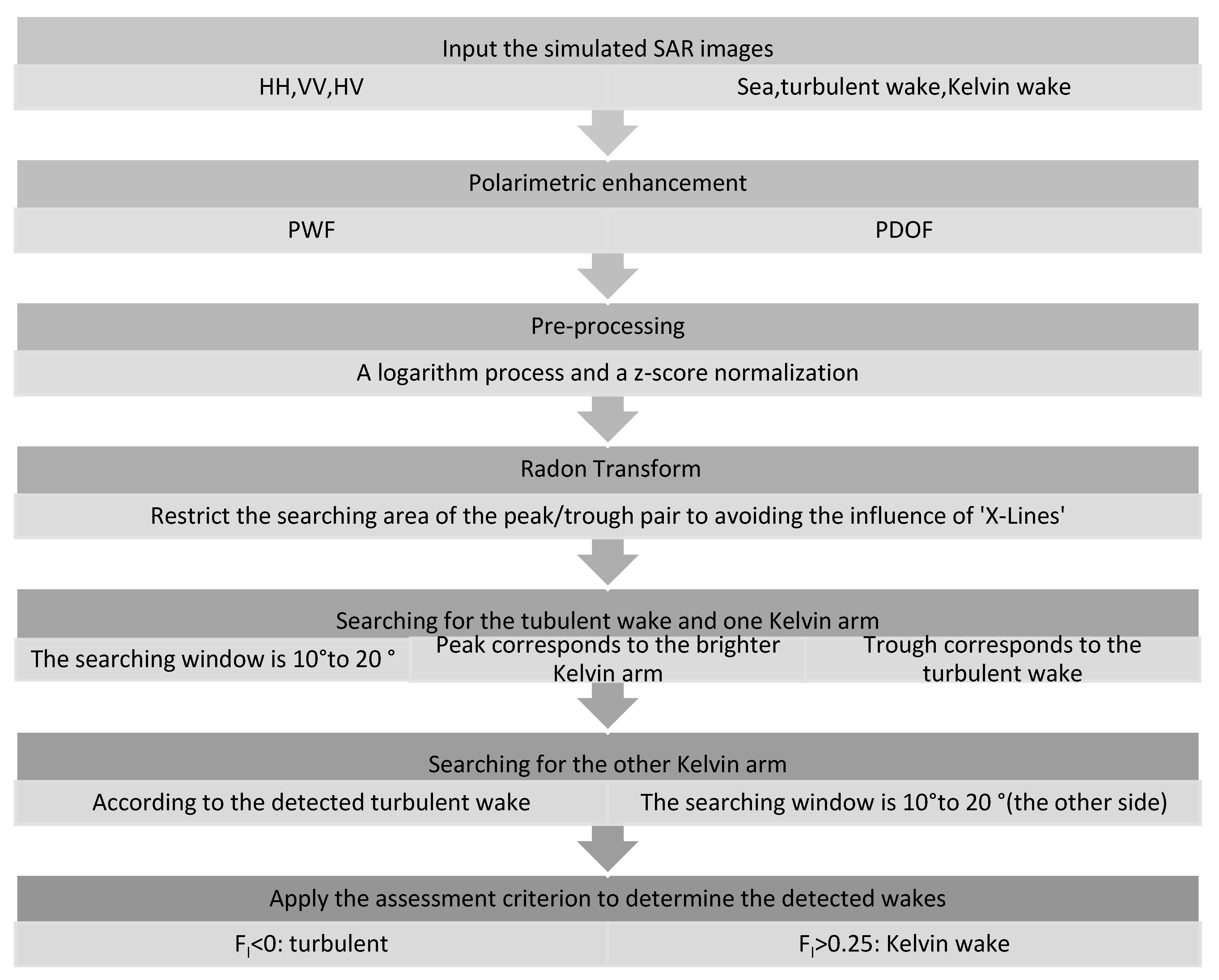
3. Methodology
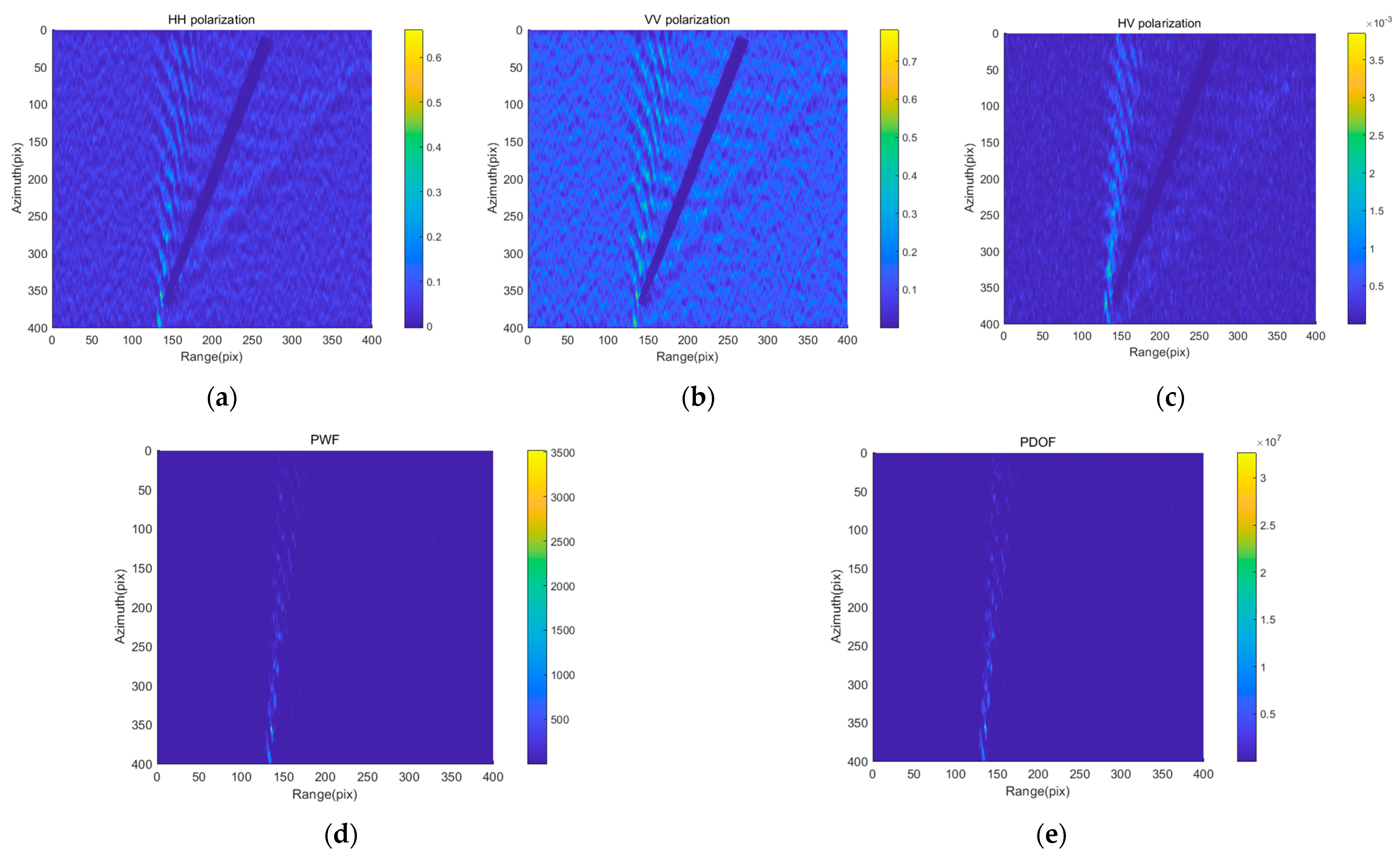
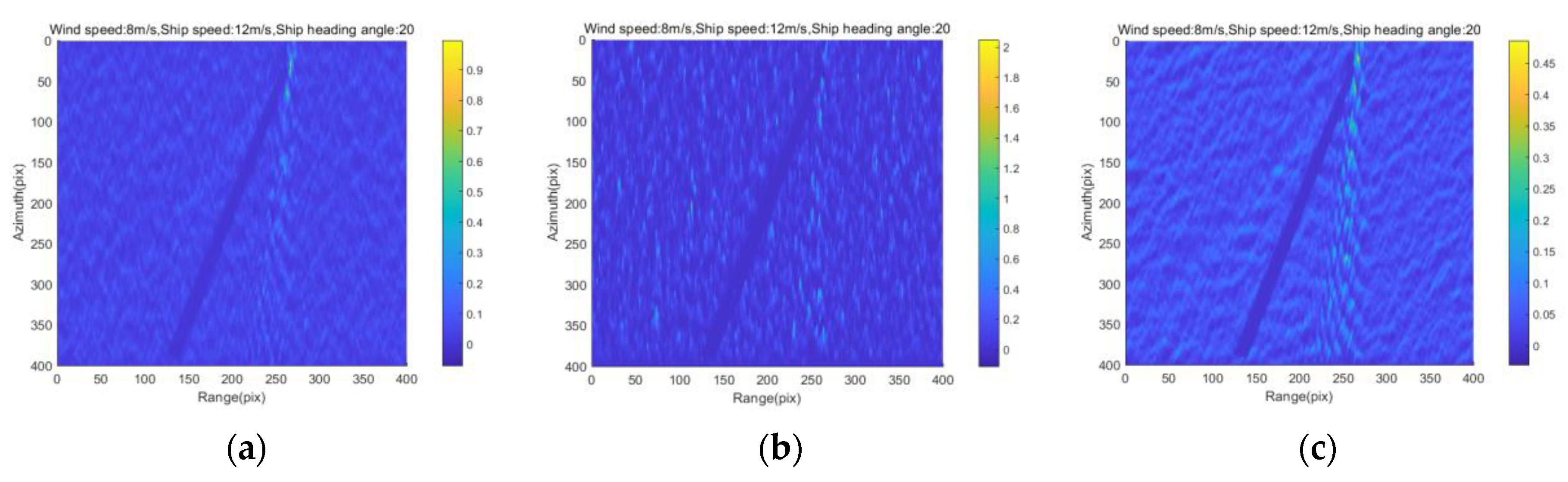
3.1. The Polarimetric Enhancement
3.2. The Pre-Processing
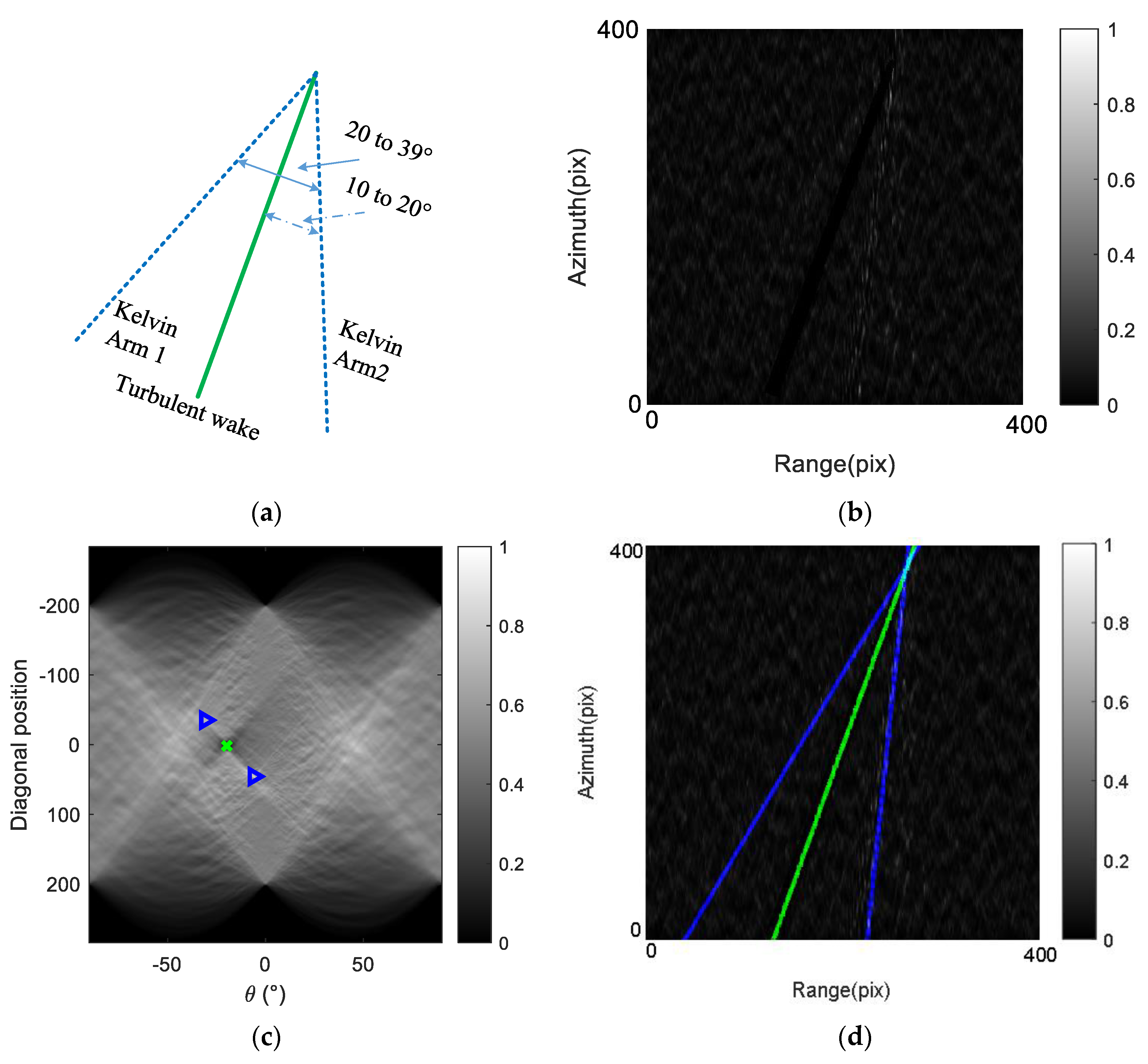
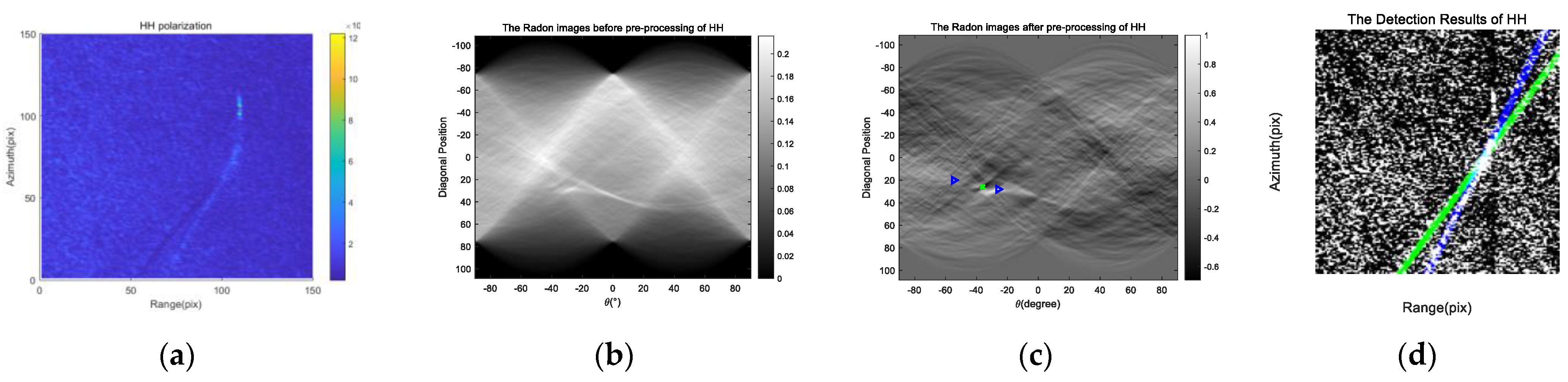
3.3. The Radon Transform and Detection Procedure
3.4. Assessment Criteria
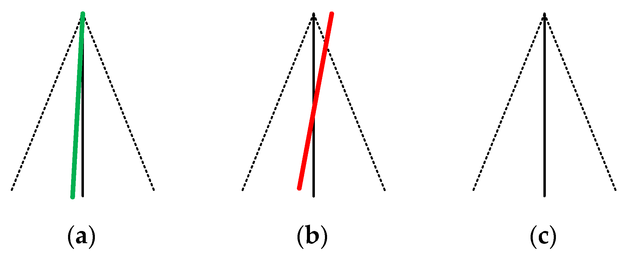
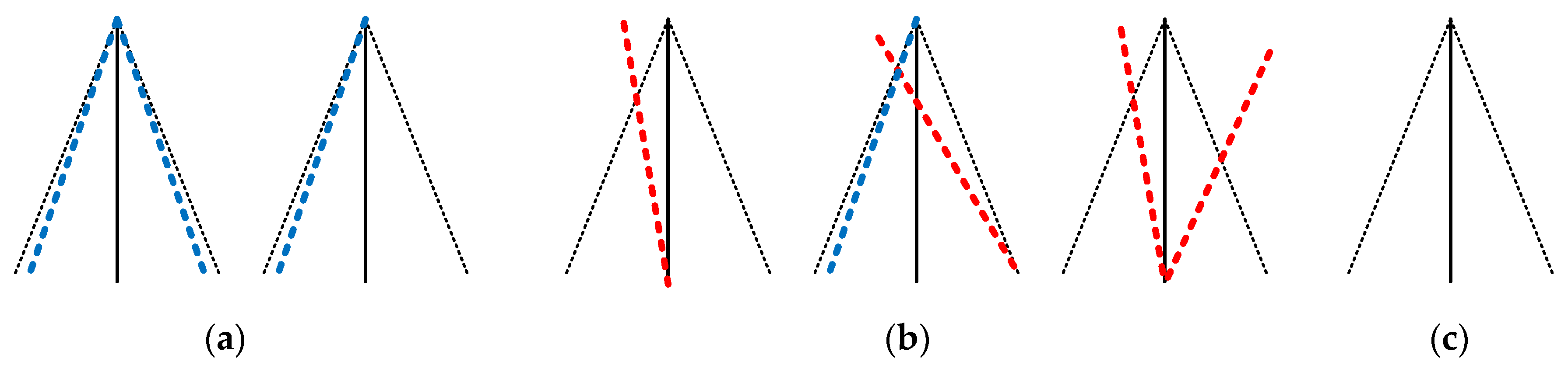
3.4.1. Confirmation of Single Wake Character
3.4.2. Detection Combination of the Kelvin and Turbulent Wake
4. Experiment and Discussion
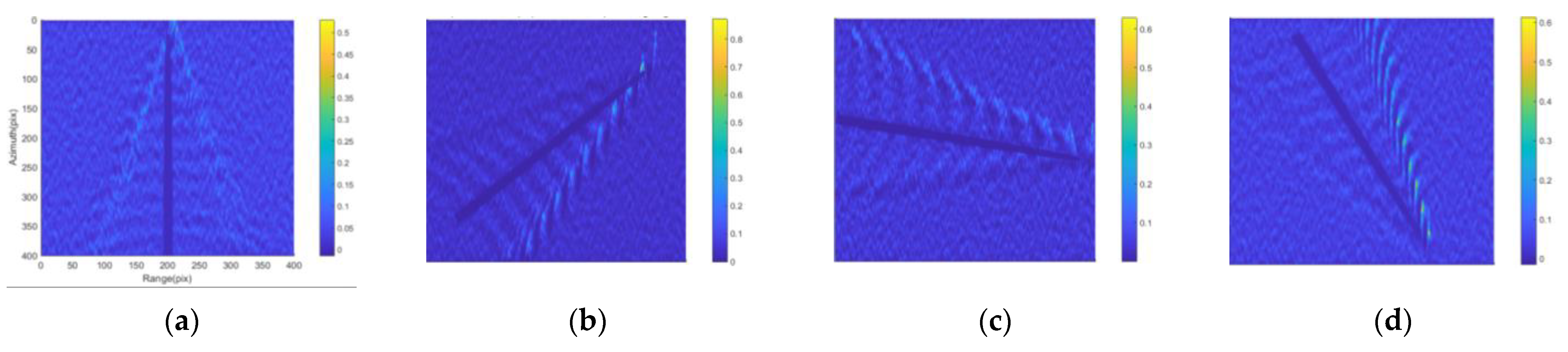
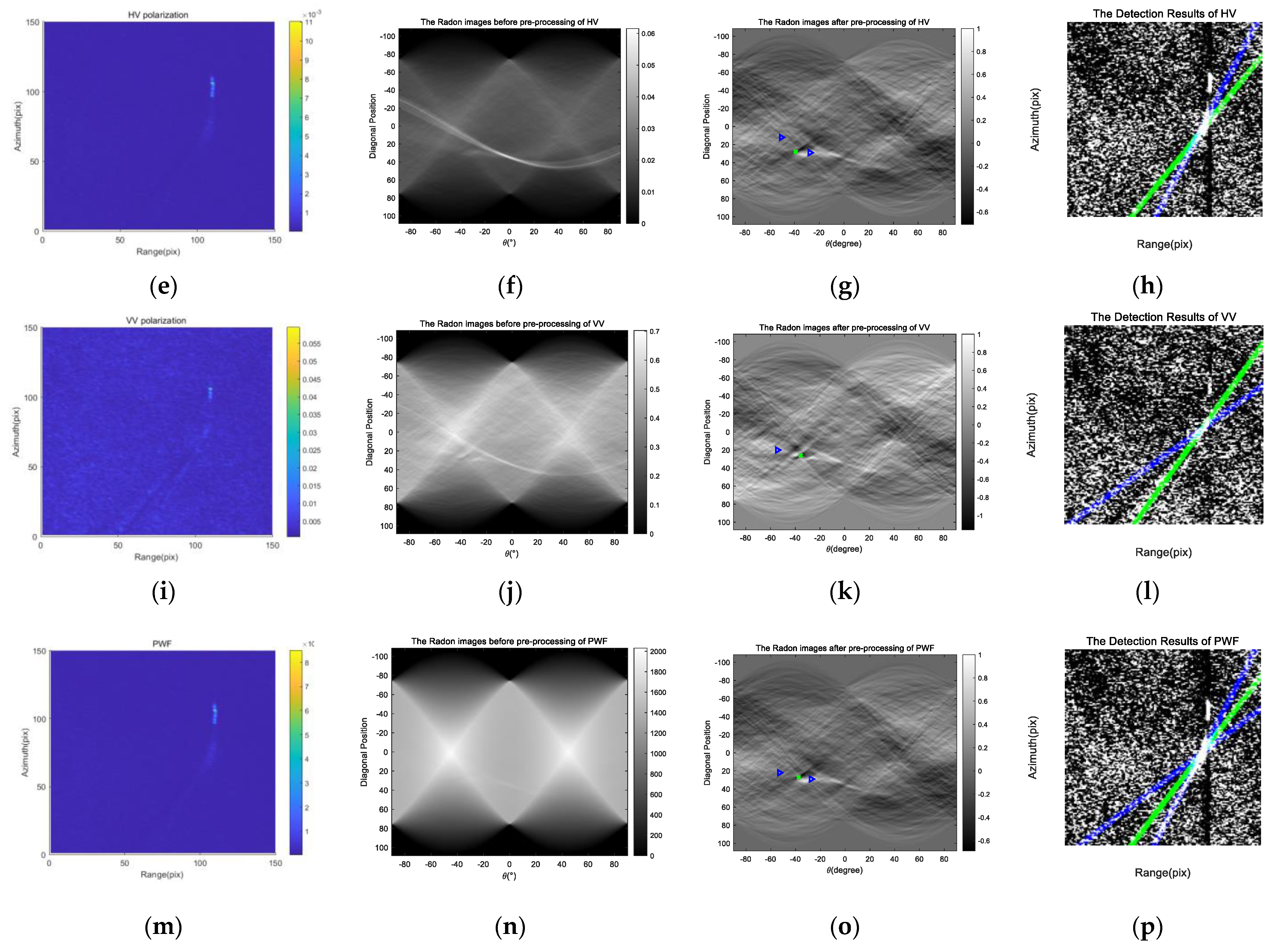
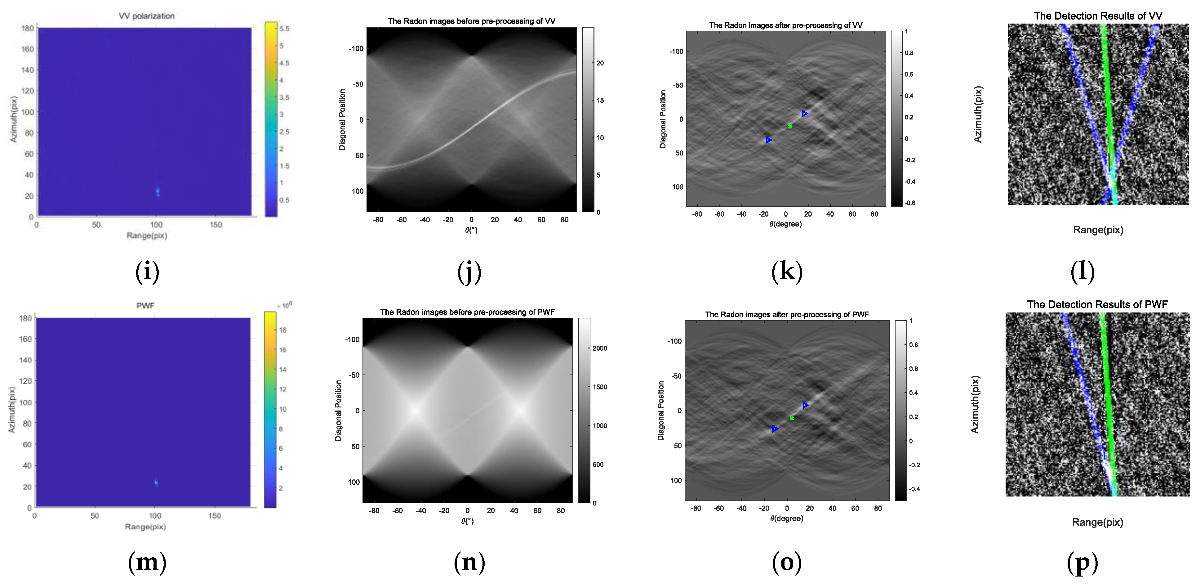
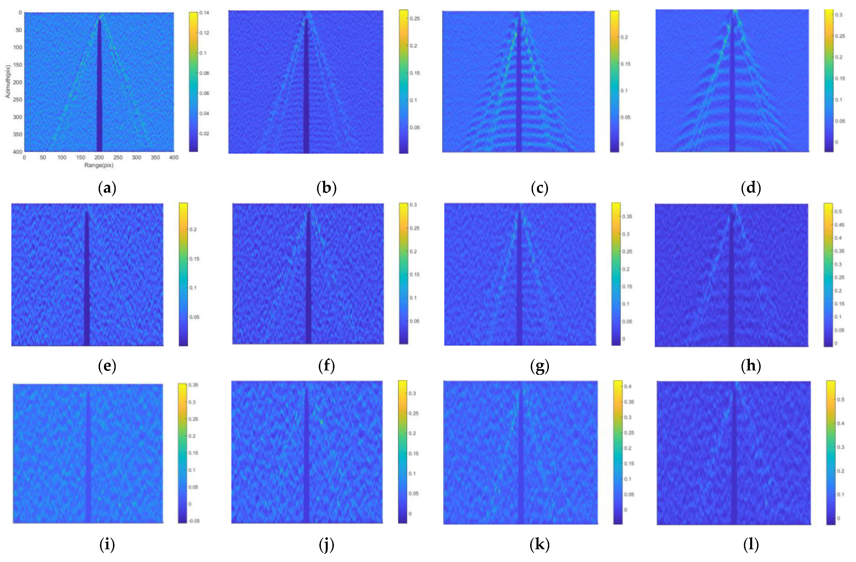
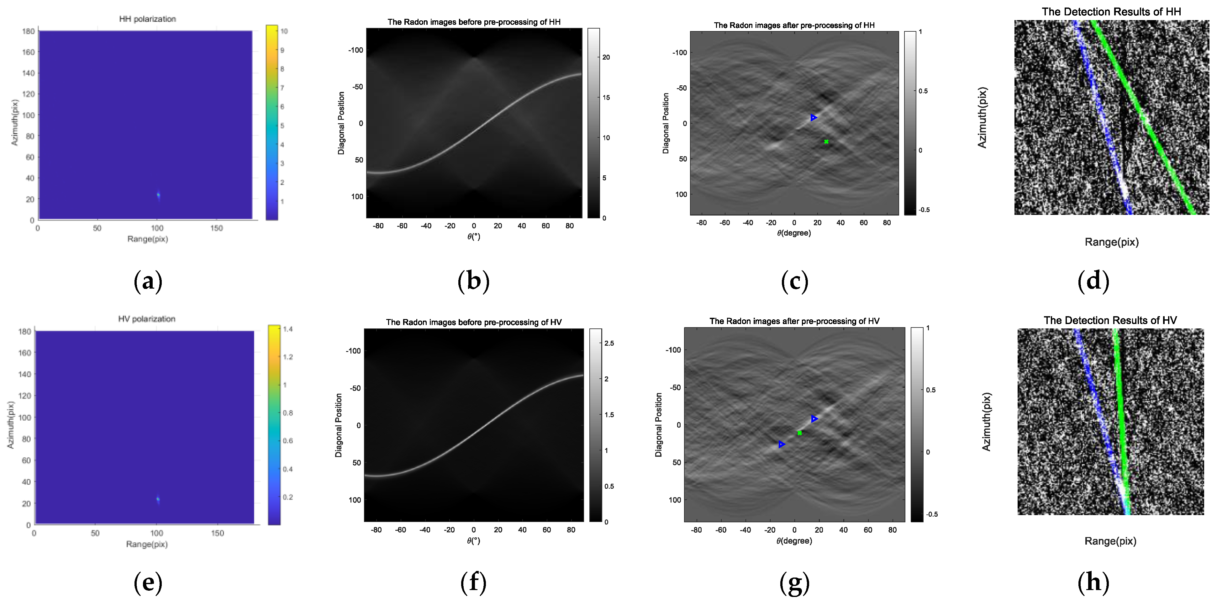
4.1. Wake Detection in the Simulated SAR Images
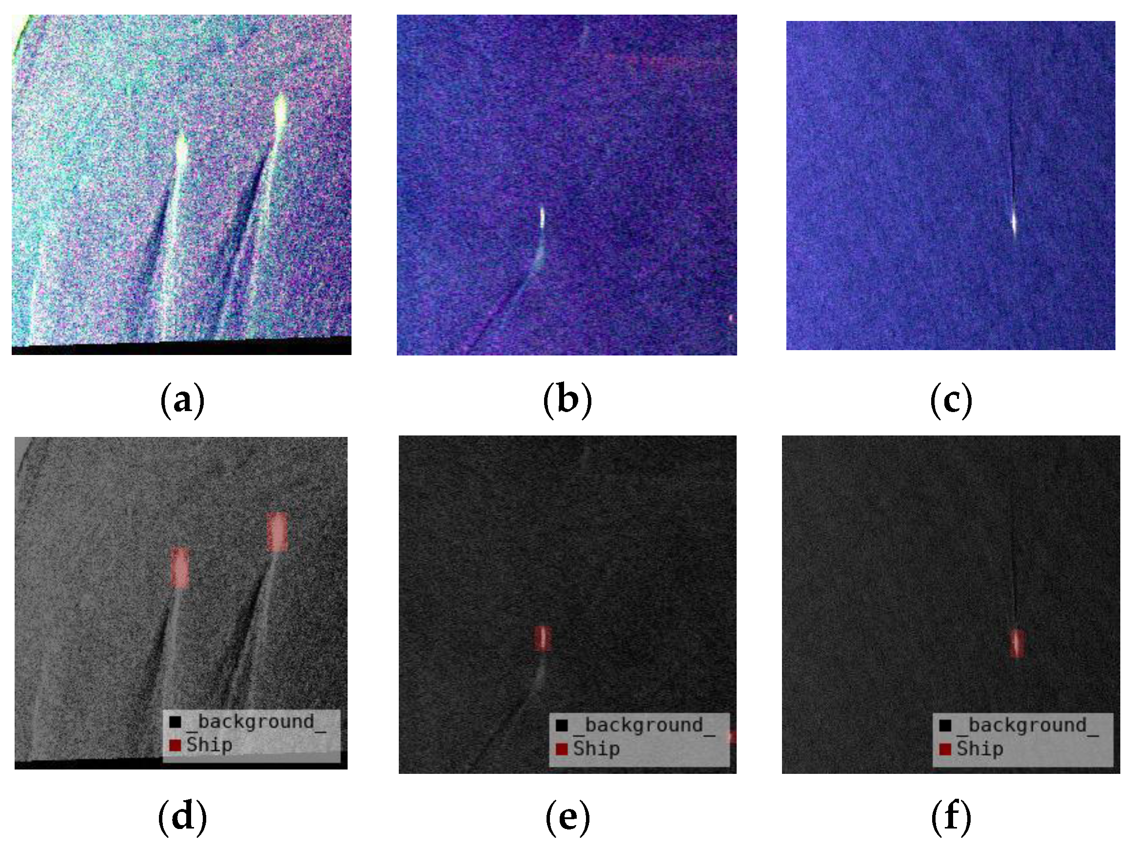
4.1.1. The Simulated Fully Polarized SAR Images
4.1.2. The Detection Results
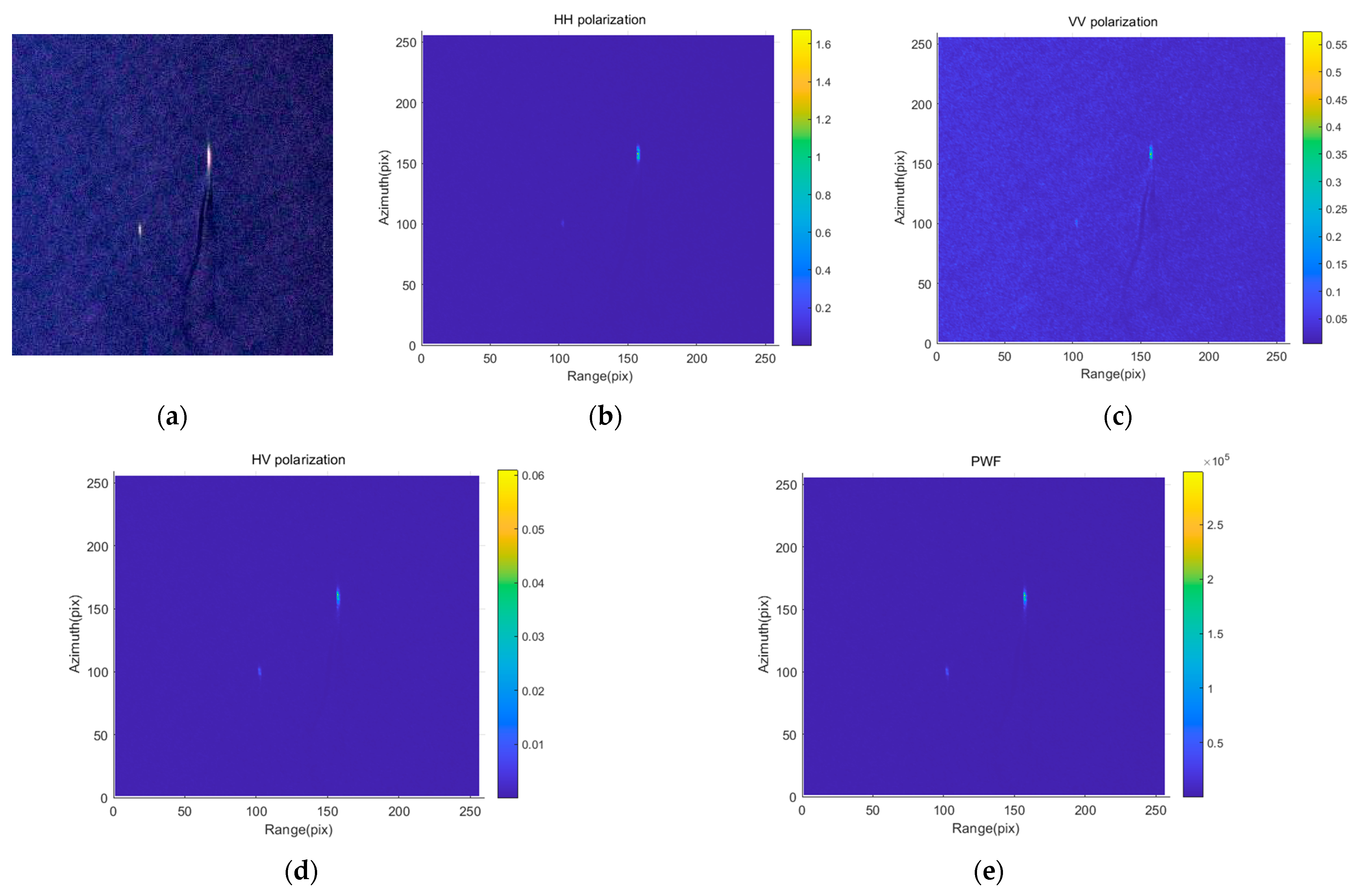
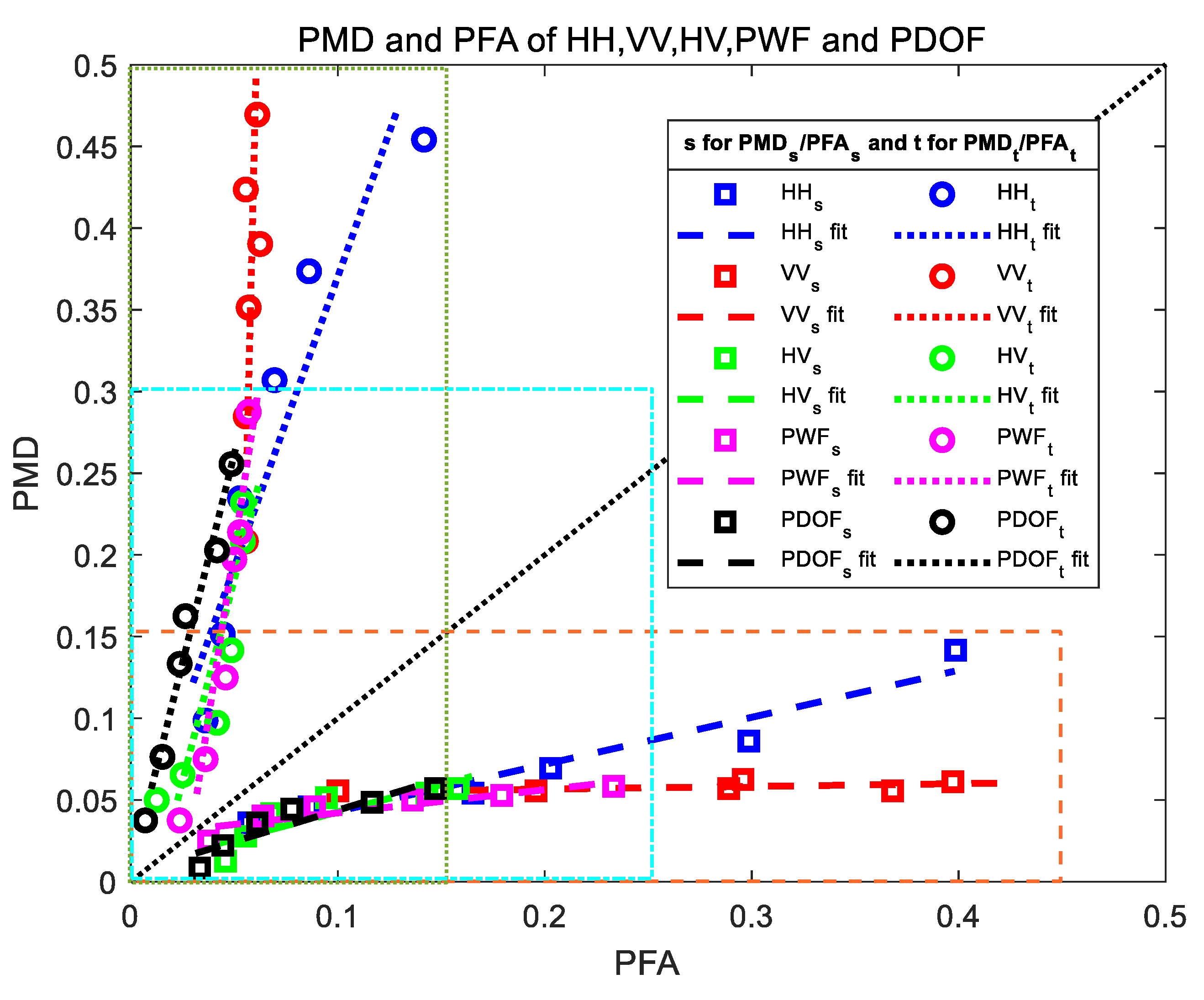
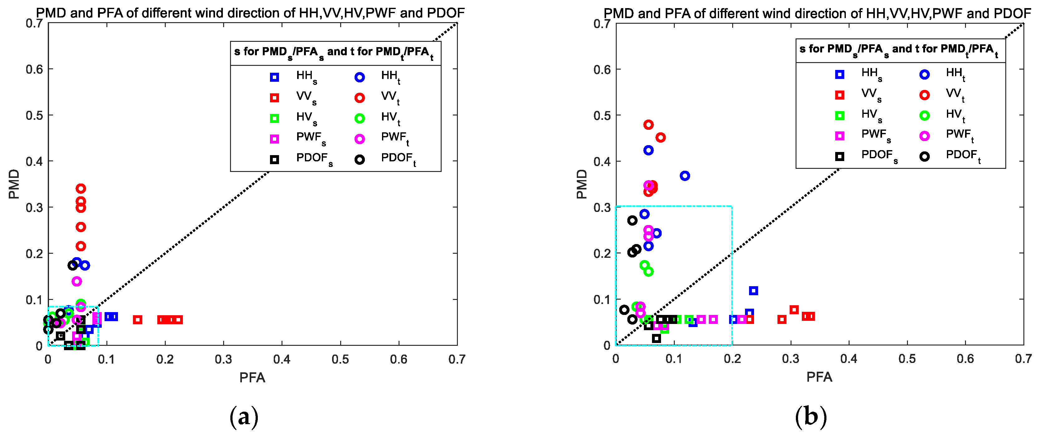
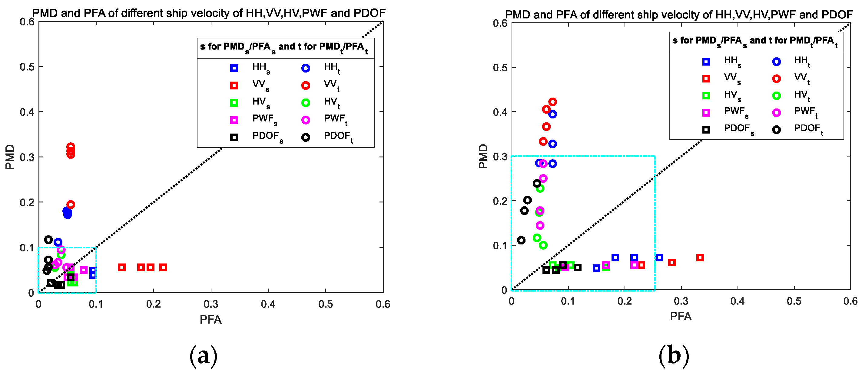
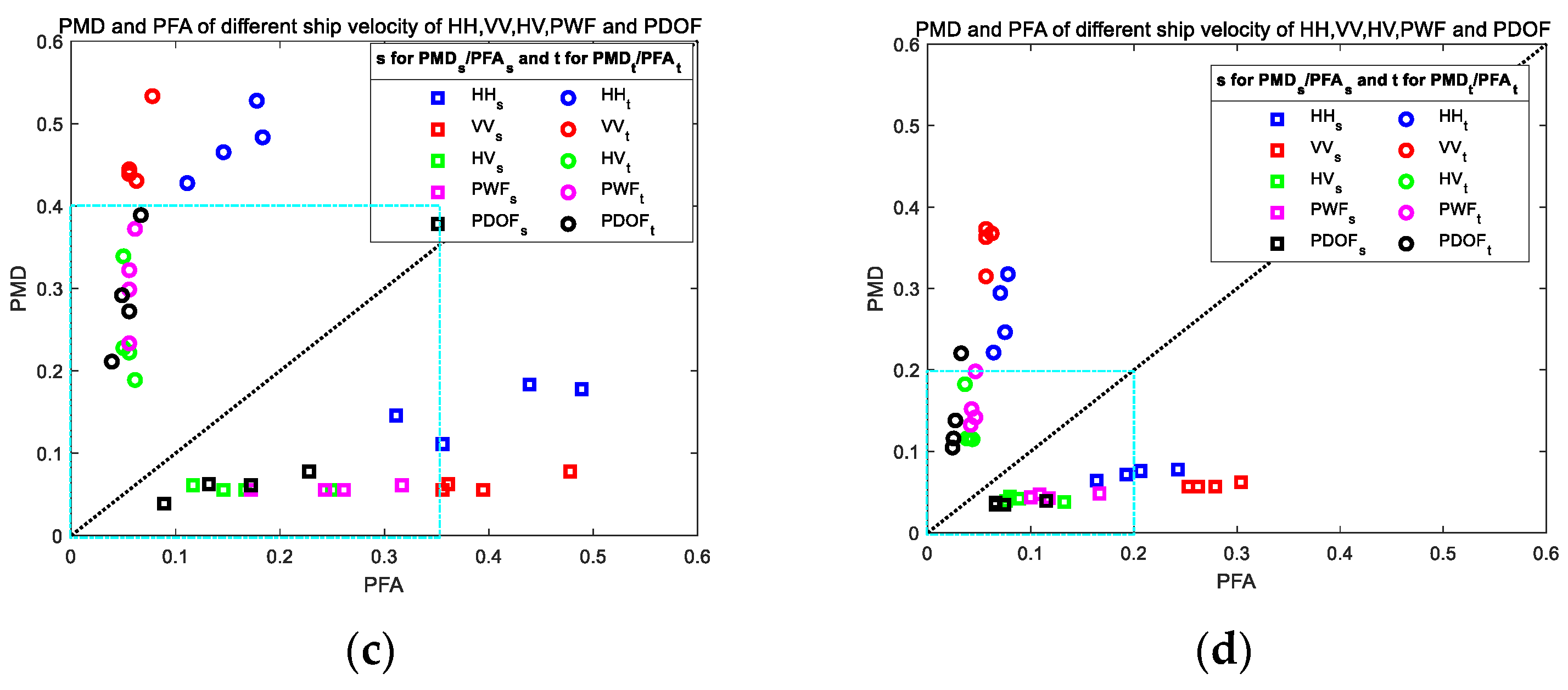
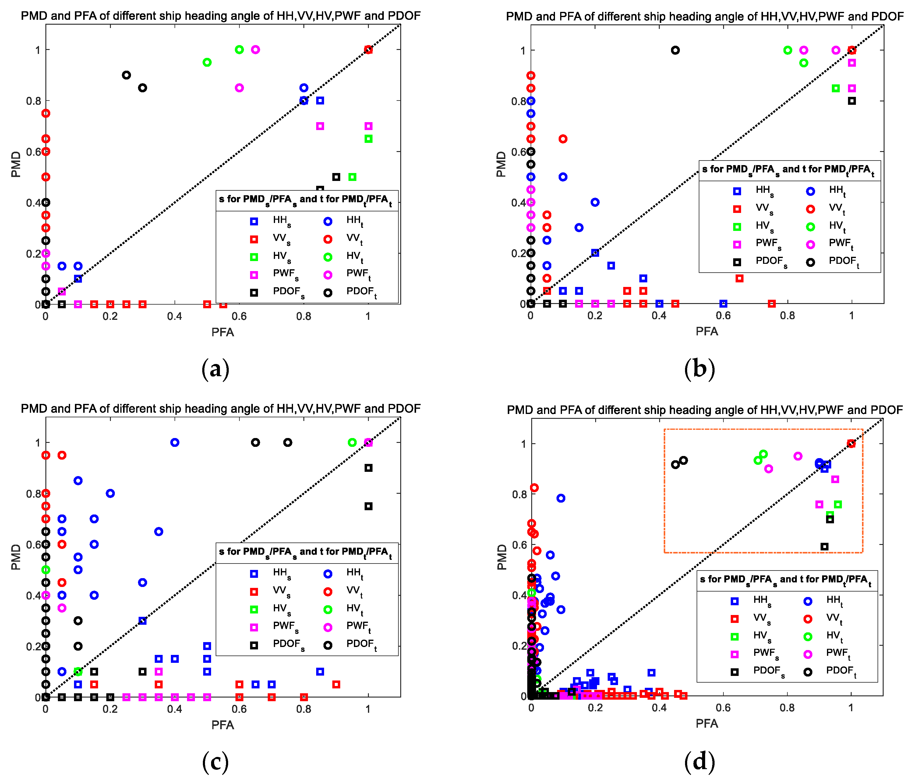
4.2. Wake Detection in the Measured SAR Images
4.3. Discussion
5. Conclusions
- (1)
- Based on the ship wake detection results, ship parameters such as ship velocity, ship heading angle and ship beam can be estimated. For different ship parameters, the wake character to be enhanced is different, and the choice of prior information of the wakes is different. In the following research, more experiments need to be carried out focusing on the choose of of the PDOF according to different situations. And deep learning algorithms need to be applied to the search of .
- (2)
- The detection performance in this paper is carried out mainly based on a large amount of simulated SAR images, and the correctness of our algorithms can be validated through the comparison of the previous similar work. The next step is to apply this algorithm to more measured SAR imagery and assess and optimize the algorithm.
- (3)
- The algorithm presented in this paper is also adaptable to the dual-pol and compact hybrid-pol scenarios [43,44], except for that only part of the information of the polarimetric covariance matrices will remain. And it is a special case of the fully polarized scenario. Therefore, the potential of dual-pol and compact hybrid-pol SAR needs to be further discovered.
Author Contributions
Funding
Data Availability Statement
Acknowledgments
Conflicts of Interest
References
- Tings, B. Non-Linear modeling of detectability of ship wake components in dependency to influencing parameters using spaceborne X-Band SAR. Remote Sens. 2021, 13, 165. [Google Scholar] [CrossRef]
- Schuler, D.L.; Lee, J.S.; Hoppel, K.; Valenzuela, G.R. Polarimetric SAR Image Signatures of Gulf-stream Features and Ship Wakes. In Proceedings of the 1992 IEEE International Geoscience and Remote Sensing Symposium, Houston, TX, USA, 26–29 May 1992. [Google Scholar]
- Pottier, E.; Boerner, W.M.; Schuler, D.L. Schuler Polarimetric Detection and Estimation of Ship Wakes. In Proceedings of the 1999 IEEE International Geoscience and Remote Sensing Symposium, Hamburg, Germany, 28 June–2 July 1999. [Google Scholar]
- Kasilingam, D.; Schuler, D.; Lee, J.S.; Malhotra, S. Modulation of Polarimetric Coherence by Ocean Features. In Proceedings of the 2002 IEEE International Geoscience and Remote Sensing Symposium, Toronto, ON, Canada, 24–28 June 2002. [Google Scholar]
- Morris, J.; Anderson, S.; Parfitt, A. Polarimetric Mapping of Ship Wakes. In Proceedings of the 2002 IEEE International Geoscience and Remote Sensing Symposium, Toronto, ON, Canada, 24–28 June 2002. [Google Scholar]
- Morris, J.; Anderson, S. An Entropy-based Approach to Wake Echo Analysis [ship wake radar detection]. In Proceedings of the 2003 International Conference on Radar, Adelaide, Australia, 3–5 September 2003. [Google Scholar]
- Yang, J.; Huang, W.; Xiao, Q.; Fu, B.; Yao, L. Optimal Polarization for the Observation of Ocean Features with SAR. In Proceedings of the 2004 IEEE International Geoscience and Remote Sensing Symposium, Anchorage, AL, USA, 20–24 September 2004. [Google Scholar]
- Wu, P.; Wang, J.; Wang, W.; Sun, J. Polarimetric Characters Extraction Research of Kelvin Wakes on PolSAR Image. In Proceedings of the 2011 International Conference on Remote Sensing, Environment and Transportation Engineering, Nanjing, China, 24–26 June 2011. [Google Scholar]
- Novak, L.M.; Sechtin, M.B.; Cardullo, M.J. Studies of target detection algorithms that use polarimetric radar data. IEEE Trans. Aerosp. Electron. Syst. 1989, 25, 150–165. [Google Scholar] [CrossRef]
- Novak, L.M.; Burl, M.C. Optimal speckle reduction in polarimetric SAR imagery. IEEE Trans. Aerosp. Electron. Syst. 1990, 26, 293–305. [Google Scholar] [CrossRef]
- Marino, A. A notch filter for ship detection with polarimetric SAR data. IEEE J. Sel. Top. Appl. Earth Obs. Remote Sens. 2013, 6, 1219–1232. [Google Scholar] [CrossRef]
- Novak, L.M.; Burl, M.C.; Irving, W.W.; Owirka, G.J. Optimal Polarimetric Processing for Enhanced Target Detection. In Proceedings of the 1991 National Telesystems Conference, Atlanta, AL, USA, 23–24 March 1991. [Google Scholar]
- Imbo, P.; Souyris, J.C.; Yeremy, M. Wake Detection in Polarimetric SAR Images. In Proceedings of the 2001 IEEE International Geoscience and Remote Sensing Symposium, Sydney, Australia, 9–13 July 2001. [Google Scholar]
- Xu, Z.; Tang, B.; Cheng, S. Faint ship wake detection in PolSAR images. IEEE Trans. Geosci. Remote Sens. 2018, 15, 1055–1059. [Google Scholar] [CrossRef]
- Biondi, F. Low-rank plus sparse decomposition and localized radon transform for ship-wake detection in synthetic aperture radar images. IEEE Geosci. Remote Sens. Lett. 2018, 15, 117–121. [Google Scholar] [CrossRef]
- Biondi, F. A polarimetric extension of low-rank plus sparse decomposition and radon transform for ship wake detection in synthetic aperture radar images. IEEE Geosci. Remote Sens. Lett. 2019, 16, 75–79. [Google Scholar] [CrossRef]
- Liu, T.; Jiang, Y.; Marino, A.; Gao, G.; Yang, J. The Polarimetric detection optimization filter and its statistical test for ship detection. IEEE Trans. Geosci. Remote Sens. 2022, 60, 1–18. [Google Scholar] [CrossRef]
- Liu, T.; Zhang, J.; Gao, G.; Yang, J.; Marino, A. CFAR ship detection in polarimetric synthetic aperture radar images based on whitening filter. IEEE Trans. Geosci. Remote Sens. 2020, 58, 58–81. [Google Scholar] [CrossRef]
- Liu, T.; Yang, Z.; Marino, A.; Gao, G.; Yang, J. PolSAR ship detection based on neighborhood polarimetric covariance matrix. IEEE Trans. Geosci. Remote Sens. 2021, 59, 4874–4887. [Google Scholar] [CrossRef]
- Liu, T.; Yang, Z.; Gao, G.; Marino, A.; Chen, S.W.; Yang, J. A general framework of polarimetric detectors based on quadratic optimization. IEEE Trans. Geosci. Remote Sens. 2022, 60, 5237418. [Google Scholar] [CrossRef]
- Liu, T.; Yang, Z.; Gao, G.; Marino, A.; Chen, S.W. Simultaneous diagonalization of Hermitian matrices and its application in PolSAR ship detection. IEEE Trans. Geosci. Remote Sens. 2023, 61, 5220818. [Google Scholar] [CrossRef]
- Liu, T.; Tang, T.; Yang, Z.; Jiang, Y. L-distribution for multilook polarimetric SAR data and its application in ship detection. Sci. China Inf. Sci. 2021, 12, 226–238. [Google Scholar]
- Deng, Y.; Zhang, M.; Jiang, W.; Wang, L. Electromagnetic scattering of near-field turbulent wake generated by accelerated propeller. Remote Sens. 2021, 13, 5178. [Google Scholar] [CrossRef]
- Wang, J.; Guo, L.; Wei, Y.; Chai, S. Study on ship Kelvin wake detection in numerically simulated SAR images. Remote Sens. 2023, 15, 1089. [Google Scholar] [CrossRef]
- Zilman, G.; Zapolski, A.; Marom, M. On detectability of a ship’s kelvin wake in simulated sar images of rough sea surface. IEEE Trans. Geosci. Remote Sens. 2015, 53, 609–619. [Google Scholar] [CrossRef]
- Rizaev, I.G.; Karakuş, O.; Hogan, S.J.; Achim, A. Modeling and SAR imaging of the sea surface: A review of the state-of-the-art with simulations. ISPRS J. Photogramm. Remote Sens. 2022, 187, 120–140. [Google Scholar] [CrossRef]
- Yang, Z.; Zhang, P.; Wang, N.; Liu, T. A lightweight theory driven network and its validation on public fully polarized ship detection dataset. IEEE J. Sel. Top. Appl. Earth Obs. Remote Sens. 2024, 17, 3755–3767. [Google Scholar] [CrossRef]
- Tings, B. Extension of ship wake detectability model for non-linear influences of parameters using satellite based X-band synthetic aperture radar. Remote Sens. 2019, 11, 563. [Google Scholar] [CrossRef]
- Karakuş, O.; Rizaev, I.; Achim, A. Ship wake detection in SAR images via sparse regularization. IEEE Trans. Geosci. Remote Sens. 2020, 58, 1665–1677. [Google Scholar] [CrossRef]
- Tings, B.; Pleskachevsky, A.; Wiehle, S. Comparison of detectability of ship wake components between C-Band and X-Band synthetic aperture radar sensors operating under different slant ranges. ISPRS J. Photogramm. Remote Sens. 2023, 196, 306–324. [Google Scholar] [CrossRef]
- Ermakov, S.; Kapustin, I.; Lazareva, T. Ship Wake Signatures in Radar/Optical Images of the Sea Surface: Observations and Physical Mechanisms. In Proceedings of the SPIE Remote Sensing of the Ocean, Sea Ice, Coastal Waters, and Large Water Regions 2014, Amsterdam, The Netherland, 24–25 September 2014. [Google Scholar]
- Rey, M.T.; Tunaley, J.K.; Folinsbee, J.T.; Jahans, P.A.; Dixon, J.A.; Vant, M.R. Application of Radon transform techniques to wake detection in Seasat-A SAR Images. IEEE Trans. Geosci. Remote Sens. 1990, 28, 553–560. [Google Scholar] [CrossRef]
- Graziano, M.D.; D’Errico, M.; Rufino, G. Wake component detection in X-Band SAR images for ship heading and velocity estimation. Remote Sens. 2016, 8, 498. [Google Scholar] [CrossRef]
- Melsheimer, C.; Lim, H.; Shen, C. Observation and Analysis of Ship Wakes in ERS SAR and SPOT Images. In Proceedings of the 20th Asian Conference on Remote Sensing, Hong Kong, China, 22–25 November 1999. [Google Scholar]
- Zilman, G.; Zapolski, A.; Marom, M. The speed and beam of a ship from its wake’s SAR images. IEEE Trans. Geosci. Remote Sens. 2003, 42, 2335–2343. [Google Scholar] [CrossRef]
- Ren, W.J.; Liu, P.; Ren, X.C.; Jin, Y.Q. SAR image simulation of ship turbulent wake using semi-empirical energy spectrum. IEEE J. Multiscale Multiphys Comput. Techn. 2021, 6, 1–7. [Google Scholar] [CrossRef]
- Milgram, J.H.; Skop, R.A.; Peltzer, R.D.; Griffin, O.M. Modeling short sea wave energy distribution in the far wakes of ships. J. Geophys. Res. 1993, 98, 7115–7124. [Google Scholar] [CrossRef]
- Alpers, W.R.; Ross, D.B.; Rufenach, C.L. On the detectability of ocean surface waves by real and synthetic aperture radar. J. Geophys. Res. 1981, 86, 6481–6498. [Google Scholar] [CrossRef]
- Lyzenga, D.R. Numerical simulation of synthetic aperture radar image spectra for ocean waves. IEEE Trans. Geosci. Remote Sens. 1986, 6, 863–872. [Google Scholar] [CrossRef]
- Pierson, W.J.; Moskowitz, L. A proposed spectral from fully developed wind seas based on the similarity theory of SA kitaigorodsrii. J. Geophys. Res. 1964, 69, 5181–5190. [Google Scholar] [CrossRef]
- Ward, K.; Tough, R.; Watts, S. Sea Clutter: Scattering, the K Distribution and Radar Performance, 2nd ed.; The Institution of Engineering and Technology: London, UK, 2013; pp. 19–21. [Google Scholar]
- Jiang, Y.; Chen, Z.; Zhao, C. Research on Key Issues of Extracting Wind Direction from HF Surface Wave Radar Oceanic Backscatter. In Proceedings of the 2016 CIE International Conference on Radar, Guangzhou, China, 10–13 October 2016. [Google Scholar]
- Espeseth, M.M.; Brekke, C.; Anfinsen, S.N. Hybrid-polarity and reconstruction methods for sea ice with L- and C-band SAR. IEEE Geosci. Remote Sens. Lett. 2016, 13, 467–471. [Google Scholar] [CrossRef]
- Kumar, A.; Mishra, V.; Panigrahi, R.K.; Martorella, M. Application of hybrid-pol SAR in oil-spill detection. IEEE Geosci. Remote Sens. Lett. 2023, 20, 1–5. [Google Scholar] [CrossRef]


| Situation Number | Figure Examples | Kelvin Detection Result | Turbulent Detection Result |
|---|---|---|---|
| 1 |  | M | T 1 |
| 2 |  | T | M 3 |
| 3 | 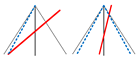 | T | F 2 |
| 4 | 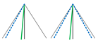 | T | T |
| 5 |  | F | T |
| 6 | 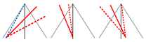 | F | F |
| 7 |  | F | M |
| 8 |  | M | F |
| 9 |  | M | M |
| Ship Parameters | Wind-Driven Sea Parameters | SAR System Parameters |
|---|---|---|
| L = 52 m, B = 5.7 m, T = 3.5 m | wind speed U10: 4:2:14 m/s | Airborne, H = 7000 m, V = 160 m/s |
| Uship: 6:2:12 m/s Ship heading angle: 0:10°:350° | PM spectrum directional spreading function: LH, S = 7 wind direction: 0°:45°:180° | Λ = 0.031 m, SAR scene: 1000 m × 1000 m, resolution: 2.5 m, radar incidence angle: 35° polarization: HH, VV, HV |
| Polarization | Wind Speed (m/s) | Wind Direction | |||||||||||
|---|---|---|---|---|---|---|---|---|---|---|---|---|---|
| 0°–180° | 0° | 45° | 90° | 135° | 180° | ||||||||
| HH | 4 | 0.0361 | 0.0569 | 0.0208 | 0.0764 | 0.0417 | 0.0625 | 0.0417 | 0.0417 | 0.0347 | 0.0486 | 0.0417 | 0.0556 |
| 6 | 0.0458 | 0.0861 | 0.0208 | 0.06254 | 0.0625 | 0.1042 | 0.0625 | 0.1111 | 0.0486 | 0.0833 | 0.0347 | 0.0694 | |
| 8 | 0.0542 | 0.16523 | 0.0556 | 0.15248 | 0.05556 | 0.1458 | 0.0556 | 0.1875 | 0.0556 | 0.1736 | 0.0486 | 0.1667 | |
| 10 | 0.0694 | 0.2028 | 0.0556 | 0.2014 | 0.1181 | 0.2361 | 0.0556 | 0.2153 | 0.0486 | 0.1319 | 0.0694 | 0.2292 | |
| 12 | 0.0861 | 0.2986 | 0.0556 | 0.3125 | 0.1597 | 0.2500 | 0.0764 | 0.3472 | 0.0833 | 0.3194 | 0.0556 | 0.2639 | |
| 14 | 0.1417 | 0.3986 | 0.0556 | 0.4167 | 0.1944 | 0.4028 | 0.2569 | 0.4861 | 0.1458 | 0.3611 | 0.0556 | 0.3264 | |
| VV | 4 | 0.0556 | 0.100 | 0.0556 | 0.1319 | 0.0556 | 0.0903 | 0.0556 | 0.0625 | 0.0556 | 0.1250 | 0.0556 | 0.0903 |
| 6 | 0.0556 | 0.1958 | 0.0556 | 0.2222 | 0.0556 | 0.2014 | 0.0556 | 0.1528 | 0.0556 | 0.1944 | 0.0556 | 0.2083 | |
| 8 | 0.0569 | 0.2889 | 0.0556 | 0.3333 | 0.0625 | 0.22224 | 0.0556 | 0.2708 | 0.0556 | 0.2986 | 0.0556 | 0.3194 | |
| 10 | 0.0625 | 0.2958 | 0.0625 | 0.3333 | 0.0764 | 0.3056 | 0.0556 | 0.2847 | 0.0556 | 0.2292 | 0.0625 | 0.3264 | |
| 12 | 0.0556 | 0.3681 | 0.0556 | 0.3681 | 0.0556 | 0.2986 | 0.0556 | 0.3611 | 0.0556 | 0.4236 | 0.0556 | 0.3889 | |
| 14 | 0.0611 | 0.3972 | 0.0556 | 0.46523 | 0.0556 | 0.2986 | 0.0764 | 0.4653 | 0.0625 | 0.3611 | 0.0556 | 0.3958 | |
| HV | 4 | 0.0125 | 0.0458 | 0 | 0.0417 | 0 | 0.0208 | 0.0278 | 0.0486 | 0.0069 | 0.0486 | 0.0278 | 0.0694 |
| 6 | 0.0278 | 0.0556 | 0 | 0.0486 | 0.0347 | 0.0556 | 0.0556 | 0.0556 | 0.0417 | 0.0556 | 0.0069 | 0.0625 | |
| 8 | 0.0417 | 0.0681 | 0.0139 | 0.0625 | 0.0556 | 0.0694 | 0.0556 | 0.0694 | 0.0556 | 0.0833 | 0.0278 | 0.0556 | |
| 10 | 0.0514 | 0.0944 | 0.0556 | 0.0556 | 0.0556 | 0.1250 | 0.0556 | 0.1042 | 0.0556 | 0.1042 | 0.0347 | 0.0833 | |
| 12 | 0.0542 | 0.1431 | 0.0486 | 0.1042 | 0.0556 | 0.1250 | 0.0556 | 0.2292 | 0.0556 | 0.1875 | 0.0556 | 0.0694 | |
| 14 | 0.0569 | 0.1583 | 0.0625 | 0.1736 | 0.0556 | 0.1667 | 0.0556 | 0.1597 | 0.0556 | 0.1458 | 0.0556 | 0.1458 | |
| PWF | 4 | 0.0250 | 0.0375 | 0.0139 | 0.0556 | 0.0139 | 0.0139 | 0.0486 | 0.0486 | 0.0208 | 0.0278 | 0.0278 | 0.0417 |
| 6 | 0.0403 | 0.0639 | 0.0069 | 0.0486 | 0.0556 | 0.0833 | 0.0625 | 0.0833 | 0.0556 | 0.0556 | 0.0208 | 0.0486 | |
| 8 | 0.0458 | 0.0889 | 0.0417 | 0.0556 | 0.0486 | 0.0764 | 0.0556 | 0.1389 | 0.0486 | 0.1181 | 0.0347 | 0.0556 | |
| 10 | 0.0500 | 0.1361 | 0.0417 | 0.0694 | 0.0556 | 0.1458 | 0.0556 | 0.2153 | 0.0556 | 0.1667 | 0.0417 | 0.0833 | |
| 12 | 0.0528 | 0.1792 | 0.0556 | 0.1111 | 0.0556 | 0.1667 | 0.0556 | 0.2708 | 0.0556 | 0.2431 | 0.0417 | 0.1042 | |
| 14 | 0.0583 | 0.2333 | 0.0625 | 0.1597 | 0.0556 | 0.1875 | 0.0625 | 0.4028 | 0.0556 | 0.2431 | 0.0556 | 0.1736 | |
| PDOF | 4 | 0.0083 | 0.0333 | 0 | 0.0278 | 0 | 0.0139 | 0.0347 | 0.0486 | 0 | 0.0278 | 0.0069 | 0.0486 |
| 6 | 0.0222 | 0.0444 | 0 | 0.0347 | 0.0347 | 0.0556 | 0.0556 | 0.0556 | 0.0208 | 0.0208 | 0 | 0.0556 | |
| 8 | 0.0361 | 0.0611 | 0.0139 | 0.0347 | 0.0556 | 0.0625 | 0.0556 | 0.1042 | 0.0556 | 0.0625 | 0 | 0.0417 | |
| 10 | 0.0444 | 0.0778 | 0.0417 | 0.0556 | 0.0556 | 0.0764 | 0.0556 | 0.0972 | 0.0556 | 0.0903 | 0.0139 | 0.0694 | |
| 12 | 0.0486 | 0.1167 | 0.0486 | 0.0694 | 0.0556 | 0.1250 | 0.0556 | 0.2014 | 0.0556 | 0.1111 | 0.0278 | 0.0764 | |
| 14 | 0.0569 | 0.1472 | 0.0625 | 0.0764 | 0.0486 | 0.1528 | 0.0556 | 0.2083 | 0.0625 | 0.1319 | 0.0556 | 0.1667 | |
| Polarization | Wind speed (m/s) | Wind Direction | |||||||||||
| 0°–180° | 0° | 45° | 90° | 135° | 180° | ||||||||
| HH | 4 | 0.0986 | 0.0361 | 0.1042 | 0.0208 | 0.1042 | 0.0417 | 0.1319 | 0.0417 | 0.0764 | 0.0347 | 0.0764 | 0.0417 |
| 6 | 0.1514 | 0.0444 | 0.0694 | 0.0208 | 0.1736 | 0.0625 | 0.2569 | 0.0556 | 0.1806 | 0.0486 | 0.0764 | 0.0347 | |
| 8 | 0.2347 | 0.0528 | 0.1667 | 0.0486 | 0.2569 | 0.0556 | 0.3333 | 0.0556 | 0.2361 | 0.0556 | 0.1806 | 0.0486 | |
| 10 | 0.3069 | 0.0694 | 0.2153 | 0.0556 | 0.3681 | 0.1181 | 0.4236 | 0.0556 | 0.2847 | 0.0486 | 0.2431 | 0.0694 | |
| 12 | 0.3736 | 0.0861 | 0.3125 | 0.0556 | 0.4097 | 0.1597 | 0.4722 | 0.0764 | 0.3889 | 0.0833 | 0.2847 | 0.0556 | |
| 14 | 0.4542 | 0.1417 | 0.4167 | 0.0556 | 0.5000 | 0.1944 | 0.5625 | 0.2569 | 0.4653 | 0.1458 | 0.3264 | 0.0556 | |
| VV | 4 | 0.2083 | 0.0556 | 0.2014 | 0.0556 | 0.1736 | 0.0556 | 0.2986 | 0.0556 | 0.2153 | 0.0556 | 0.1528 | 0.0556 |
| 6 | 0.2847 | 0.0556 | 0.2569 | 0.0556 | 0.2986 | 0.0556 | 0.3403 | 0.0556 | 0.3125 | 0.0556 | 0.2153 | 0.0556 | |
| 8 | 0.3514 | 0.0569 | 0.3472 | 0.0556 | 0.3472 | 0.0625 | 0.3889 | 0.0556 | 0.3542 | 0.0556 | 0.3194 | 0.0556 | |
| 10 | 0.3903 | 0.0625 | 0.3403 | 0.0625 | 0.4514 | 0.0764 | 0.4792 | 0.0556 | 0.3333 | 0.0556 | 0.3472 | 0.0625 | |
| 12 | 0.4236 | 0.0556 | 0.3750 | 0.0556 | 0.4167 | 0.0556 | 0.4653 | 0.0556 | 0.4722 | 0.0556 | 0.3889 | 0.0556 | |
| 14 | 0.4694 | 0.0611 | 0.4722 | 0.0556 | 0.4028 | 0.0556 | 0.6319 | 0.0764 | 0.4306 | 0.0625 | 0.4097 | 0.0556 | |
| HV | 4 | 0.0500 | 0.0125 | 0.0486 | 0 | 0.0278 | 0 | 0.0556 | 0.0278 | 0.0486 | 0.0069 | 0.0694 | 0.0278 |
| 6 | 0.0653 | 0.0250 | 0.0486 | 0 | 0.0694 | 0.0347 | 0.0903 | 0.0556 | 0.0556 | 0.0278 | 0.0625 | 0.0069 | |
| 8 | 0.0972 | 0.0417 | 0.0625 | 0.0139 | 0.1042 | 0.0556 | 0.1597 | 0.0556 | 0.1042 | 0.0556 | 0.0556 | 0.0278 | |
| 10 | 0.1417 | 0.0486 | 0.0556 | 0.0486 | 0.1597 | 0.0556 | 0.2361 | 0.0556 | 0.1736 | 0.0486 | 0.0833 | 0.0347 | |
| 12 | 0.2083 | 0.0542 | 0.1250 | 0.0486 | 0.2361 | 0.0556 | 0.3472 | 0.0556 | 0.2639 | 0.0555 | 0.0694 | 0.0556 | |
| 14 | 0.2319 | 0.0542 | 0.1875 | 0.0625 | 0.2500 | 0.0556 | 0.3452 | 0.0417 | 0.2222 | 0.0556 | 0.1458 | 0.0556 | |
| PWF | 4 | 0.0375 | 0.0236 | 0.0556 | 0.0139 | 0.0139 | 0.0069 | 0.0486 | 0.0486 | 0.0278 | 0.0208 | 0.0417 | 0.0278 |
| 6 | 0.0750 | 0.0361 | 0.0486 | 0.0069 | 0.0833 | 0.0556 | 0.1389 | 0.0486 | 0.0556 | 0.0486 | 0.0486 | 0.0208 | |
| 8 | 0.1250 | 0.0458 | 0.0625 | 0.0417 | 0.1250 | 0.0486 | 0.2361 | 0.0556 | 0.1458 | 0.0486 | 0.0556 | 0.0347 | |
| 10 | 0.1972 | 0.0500 | 0.0694 | 0.0417 | 0.2361 | 0.0556 | 0.3472 | 0.0556 | 0.2500 | 0.0556 | 0.0833 | 0.0417 | |
| 12 | 0.2139 | 0.0528 | 0.1250 | 0.0556 | 0.2500 | 0.0556 | 0.3194 | 0.0556 | 0.2708 | 0.0556 | 0.1042 | 0.0417 | |
| 14 | 0.2875 | 0.0569 | 0.1597 | 0.0625 | 0.2500 | 0.0556 | 0.5556 | 0.0556 | 0.2986 | 0.0556 | 0.1736 | 0.0556 | |
| PDOF | 4 | 0.0375 | 0.0069 | 0.0278 | 0 | 0.0139 | 0 | 0.0694 | 0.0278 | 0.0278 | 0 | 0.0486 | 0.0069 |
| 6 | 0.0764 | 0.0153 | 0.0347 | 0 | 0.0694 | 0.0208 | 0.1736 | 0.0417 | 0.0486 | 0.0139 | 0.0556 | 0 | |
| 8 | 0.1333 | 0.0236 | 0.0347 | 0.0139 | 0.1597 | 0.0347 | 0.2917 | 0.0486 | 0.1319 | 0.0208 | 0.0486 | 0 | |
| 10 | 0.1625 | 0.0264 | 0.0556 | 0.0278 | 0.2083 | 0.0347 | 0.2708 | 0.0278 | 0.2014 | 0.0278 | 0.0764 | 0.0139 | |
| 12 | 0.2028 | 0.0417 | 0.0903 | 0.0417 | 0.3056 | 0.0556 | 0.3264 | 0.0417 | 0.2153 | 0.0417 | 0.0764 | 0.0278 | |
| 14 | 0.2556 | 0.0486 | 0.0972 | 0.0625 | 0.2847 | 0.0486 | 0.4306 | 0.0278 | 0.2917 | 0.0486 | 0.1736 | 0.0556 | |
| Polarization | U10 (m/s) | Ship Velocity (m/s) | |||||||||||||||
|---|---|---|---|---|---|---|---|---|---|---|---|---|---|---|---|---|---|
| 6 | 8 | 10 | 12 | ||||||||||||||
| HH | 4 | 0.017 | 0.039 | 0.083 | 0.017 | 0.022 | 0.050 | 0.056 | 0.022 | 0.044 | 0.072 | 0.150 | 0.044 | 0.061 | 0.067 | 0.106 | 0.061 |
| 6 | 0.050 | 0.078 | 0.172 | 0.050 | 0.039 | 0.094 | 0.111 | 0.033 | 0.050 | 0.078 | 0.178 | 0.050 | 0.044 | 0.094 | 0.144 | 0.044 | |
| 8 | 0.050 | 0.222 | 0.300 | 0.050 | 0.056 | 0.167 | 0.200 | 0.056 | 0.056 | 0.161 | 0.278 | 0.050 | 0.056 | 0.111 | 0.161 | 0.056 | |
| 10 | 0.072 | 0.261 | 0.394 | 0.072 | 0.072 | 0.217 | 0.283 | 0.072 | 0.072 | 0.183 | 0.328 | 0.072 | 0.061 | 0.150 | 0.222 | 0.061 | |
| 12 | 0.100 | 0.367 | 0.428 | 0.100 | 0.083 | 0.272 | 0.344 | 0.083 | 0.094 | 0.306 | 0.406 | 0.094 | 0.067 | 0.250 | 0.317 | 0.067 | |
| 14 | 0.178 | 0.489 | 0.528 | 0.178 | 0.183 | 0.439 | 0.483 | 0.183 | 0.111 | 0.356 | 0.428 | 0.111 | 0.094 | 0.311 | 0.378 | 0.094 | |
| VV | 4 | 0.056 | 0.072 | 0.133 | 0.056 | 0.056 | 0.094 | 0.156 | 0.056 | 0.056 | 0.072 | 0.256 | 0.056 | 0.056 | 0.161 | 0.289 | 0.056 |
| 6 | 0.056 | 0.217 | 0.306 | 0.056 | 0.056 | 0.144 | 0.194 | 0.056 | 0.056 | 0.178 | 0.322 | 0.056 | 0.056 | 0.244 | 0.317 | 0.056 | |
| 8 | 0.056 | 0.311 | 0.306 | 0.056 | 0.056 | 0.283 | 0.322 | 0.056 | 0.056 | 0.294 | 0.383 | 0.056 | 0.061 | 0.267 | 0.344 | 0.061 | |
| 10 | 0.072 | 0.333 | 0.422 | 0.072 | 0.061 | 0.283 | 0.367 | 0.061 | 0.061 | 0.283 | 0.406 | 0.061 | 0.056 | 0.283 | 0.367 | 0.056 | |
| 12 | 0.056 | 0.411 | 0.456 | 0.056 | 0.056 | 0.372 | 0.411 | 0.056 | 0.056 | 0.333 | 0.428 | 0.056 | 0.056 | 0.356 | 0.400 | 0.056 | |
| 14 | 0.078 | 0.478 | 0.533 | 0.078 | 0.056 | 0.394 | 0.439 | 0.056 | 0.056 | 0.356 | 0.444 | 0.056 | 0.056 | 0.361 | 0.461 | 0.056 | |
| HV | 4 | 0.006 | 0.044 | 0.044 | 0.006 | 0.017 | 0.044 | 0.050 | 0.017 | 0.017 | 0.044 | 0.056 | 0.017 | 0.011 | 0.050 | 0.050 | 0.011 |
| 6 | 0.023 | 0.061 | 0.072 | 0.017 | 0.022 | 0.056 | 0.056 | 0.017 | 0.039 | 0.056 | 0.083 | 0.039 | 0.028 | 0.050 | 0.050 | 0.028 | |
| 8 | 0.039 | 0.078 | 0.133 | 0.039 | 0.044 | 0.061 | 0.078 | 0.044 | 0.044 | 0.061 | 0.078 | 0.044 | 0.039 | 0.072 | 0.100 | 0.039 | |
| 10 | 0.050 | 0.167 | 0.228 | 0.050 | 0.056 | 0.072 | 0.100 | 0.056 | 0.050 | 0.083 | 0.117 | 0.044 | 0.050 | 0.056 | 0.122 | 0.044 | |
| 12 | 0.056 | 0.194 | 0.278 | 0.056 | 0.056 | 0.133 | 0.189 | 0.056 | 0.056 | 0.117 | 0.167 | 0.056 | 0.050 | 0.128 | 0.200 | 0.050 | |
| 14 | 0.056 | 0.250 | 0.339 | 0.050 | 0.056 | 0.167 | 0.228 | 0.050 | 0.061 | 0.117 | 0.189 | 0.061 | 0.056 | 0.100 | 0.172 | 0.056 | |
| PWF | 4 | 0.028 | 0.033 | 0.033 | 0.028 | 0.017 | 0.039 | 0.039 | 0.017 | 0.022 | 0.028 | 0.028 | 0.017 | 0.033 | 0.050 | 0.050 | 0.033 |
| 6 | 0.050 | 0.078 | 0.094 | 0.039 | 0.033 | 0.061 | 0.067 | 0.033 | 0.033 | 0.050 | 0.061 | 0.028 | 0.044 | 0.067 | 0.078 | 0.044 | |
| 8 | 0.039 | 0.128 | 0.156 | 0.039 | 0.044 | 0.078 | 0.122 | 0.044 | 0.050 | 0.072 | 0.106 | 0.050 | 0.050 | 0.078 | 0.117 | 0.050 | |
| 10 | 0.056 | 0.217 | 0.283 | 0.056 | 0.050 | 0.117 | 0.178 | 0.005 | 0.050 | 0.094 | 0.144 | 0.050 | 0.044 | 0.117 | 0.183 | 0.044 | |
| 12 | 0.056 | 0.228 | 0.250 | 0.056 | 0.056 | 0.150 | 0.183 | 0.056 | 0.050 | 0.183 | 0.222 | 0.050 | 0.050 | 0.156 | 0.200 | 0.050 | |
| 14 | 0.061 | 0.317 | 0.372 | 0.061 | 0.056 | 0.261 | 0.322 | 0.056 | 0.056 | 0.172 | 0.233 | 0.056 | 0.061 | 0.183 | 0.222 | 0.056 | |
| PDOF | 4 | 0.0056 | 0.039 | 0.050 | 0 | 0.0056 | 0.017 | 0.022 | 0.006 | 0.017 | 0.050 | 0.050 | 0.017 | 0.006 | 0.028 | 0.028 | 0.006 |
| 6 | 0.017 | 0.039 | 0.117 | 0.017 | 0.017 | 0.033 | 0.056 | 0.017 | 0.033 | 0.056 | 0.072 | 0.017 | 0.022 | 0.050 | 0.061 | 0.011 | |
| 8 | 0.033 | 0.078 | 0.211 | 0.022 | 0.033 | 0.050 | 0.128 | 0.022 | 0.039 | 0.050 | 0.089 | 0.022 | 0.039 | 0.067 | 0.106 | 0.028 | |
| 10 | 0.050 | 0.117 | 0.239 | 0.044 | 0.044 | 0.078 | 0.178 | 0.022 | 0.044 | 0.061 | 0.111 | 0.017 | 0.039 | 0.056 | 0.122 | 0.022 | |
| 12 | 0.050 | 0.189 | 0.317 | 0.044 | 0.044 | 0.094 | 0.172 | 0.039 | 0.050 | 0.089 | 0.161 | 0.039 | 0.050 | 0.094 | 0.161 | 0.044 | |
| 14 | 0.078 | 0.228 | 0.389 | 0.067 | 0.061 | 0.172 | 0.272 | 0.056 | 0.039 | 0.089 | 0.211 | 0.039 | 0.050 | 0.100 | 0.150 | 0.033 | |
Disclaimer/Publisher’s Note: The statements, opinions and data contained in all publications are solely those of the individual author(s) and contributor(s) and not of MDPI and/or the editor(s). MDPI and/or the editor(s) disclaim responsibility for any injury to people or property resulting from any ideas, methods, instructions or products referred to in the content. |
© 2024 by the authors. Licensee MDPI, Basel, Switzerland. This article is an open access article distributed under the terms and conditions of the Creative Commons Attribution (CC BY) license (https://creativecommons.org/licenses/by/4.0/).
Share and Cite
Jiang, Y.; Yang, Z.; Li, K.; Liu, T. Pre-Processing of Simulated Synthetic Aperture Radar Image Scenes Using Polarimetric Enhancement for Improved Ship Wake Detection. Remote Sens. 2024, 16, 658. https://doi.org/10.3390/rs16040658
Jiang Y, Yang Z, Li K, Liu T. Pre-Processing of Simulated Synthetic Aperture Radar Image Scenes Using Polarimetric Enhancement for Improved Ship Wake Detection. Remote Sensing. 2024; 16(4):658. https://doi.org/10.3390/rs16040658
Chicago/Turabian StyleJiang, Yanni, Ziyuan Yang, Ke Li, and Tao Liu. 2024. "Pre-Processing of Simulated Synthetic Aperture Radar Image Scenes Using Polarimetric Enhancement for Improved Ship Wake Detection" Remote Sensing 16, no. 4: 658. https://doi.org/10.3390/rs16040658
APA StyleJiang, Y., Yang, Z., Li, K., & Liu, T. (2024). Pre-Processing of Simulated Synthetic Aperture Radar Image Scenes Using Polarimetric Enhancement for Improved Ship Wake Detection. Remote Sensing, 16(4), 658. https://doi.org/10.3390/rs16040658