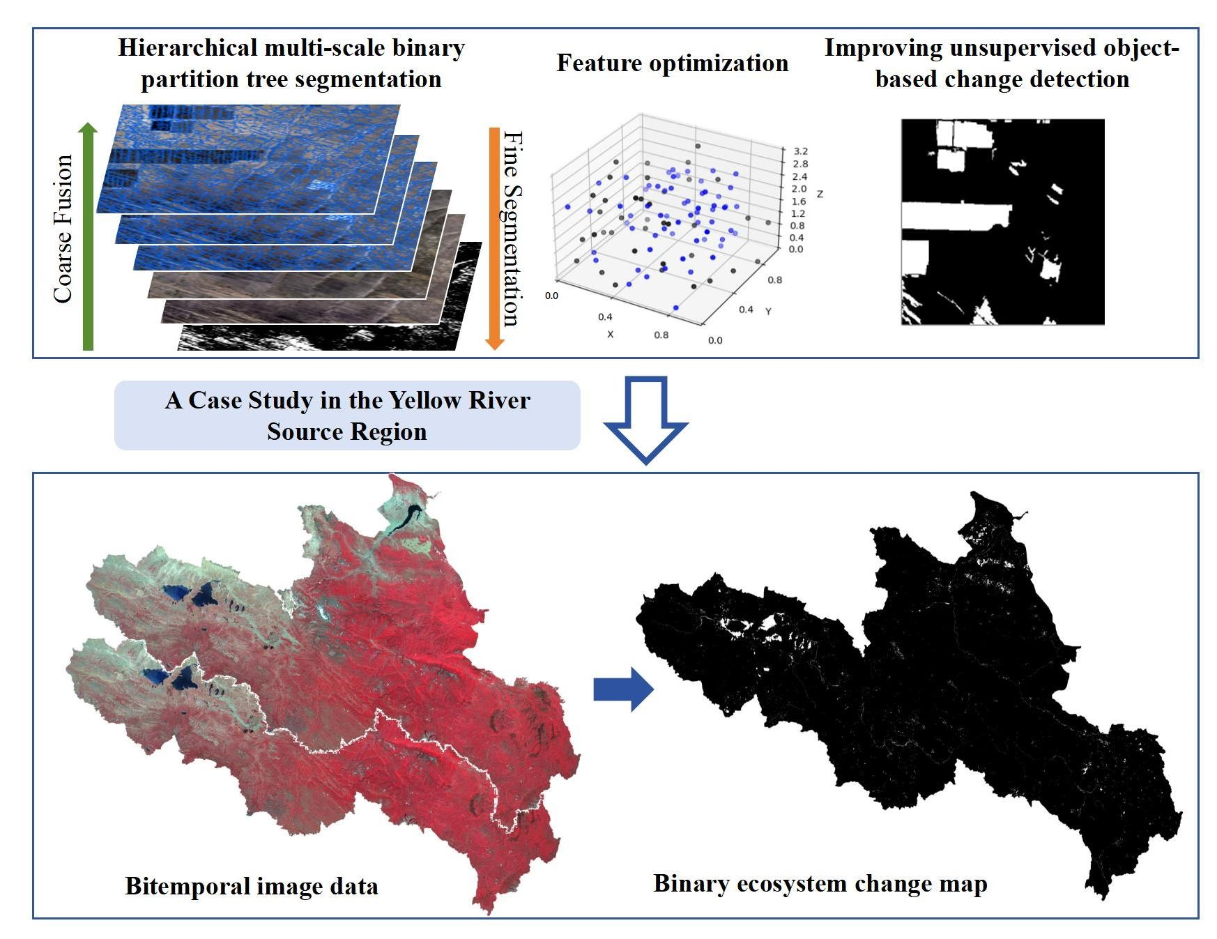
Improving Unsupervised Object-Based Change Detection via Hierarchical Multi-Scale Binary Partition Tree Segmentation: A Case Study in the Yellow River Source Region

Abstract

Change detection in remote sensing enables identifying alterations in surface characteristics over time, underpinning diverse applications. However, conventional pixel-based algorithms encounter constraints in terms of accuracy when applied to medium- and high-resolution remote sensing images. Although object-oriented methods offer a step forward, they frequently grapple with missing small objects or handling complex features effectively. To bridge these gaps, this paper proposes an unsupervised object-oriented change detection approach empowered by hierarchical multi-scale segmentation for generating binary ecosystem change maps. This approach meticulously segments images into optimal sizes and leverages multidimensional features to adapt the Iteratively Reweighted Multivariate Alteration Detection (IRMAD) algorithm for GaoFen WFV data. We rigorously evaluated its performance in the Yellow River Source Region, a critical ecosystem conservation zone. The results unveil three key strengths: (1) the approach achieved excellent object-level change detection results, making it particularly suited for identifying changes in subtle features; (2) while simply increasing object features did not lead to a linear accuracy gain, optimized feature space construction effectively mitigated dimensionality issues; and (3) the scalability of our approach is underscored by its success in mapping the entire Yellow River Source Region, achieving an overall accuracy of 90.09% and F-score of 0.8844. Furthermore, our analysis reveals that from 2015 to 2022, changed ecosystems comprised approximately 1.42% of the total area, providing valuable insights into regional ecosystem dynamics.

1. Introduction

The increasing development of remote sensing satellite imaging technology enables the dynamic monitoring of surface ecosystem and human activity changes [1], making it invaluable for ecosystem assessments, disaster monitoring, and land management [2,3,4]. Change detection (CD) is the process of identifying differences in the state of an object by analyzing a sequence of images acquired at different times.

For optical sensors, current CD methods mainly fall under the categories of pixel-based change detection (PBCD) and object-oriented change detection (OBCD) [1]. PBCD methods perform well in identifying subtle changes because of high precision of unit analysis [5]. However, as spatial resolution improves, richer spatial features bring about more complex analysis needs. The performance of PBCD algorithms is often limited by texture similarity among different ground surface objects, spatial heterogeneity within the same object, and the “salt and pepper” effect at the pixel level [6,7].

OBCD methods combine ground objects and adjacent pixels with homogeneous characteristics into a basic input unit to identify the locations and types of the change areas. The results of OBCD methods are consistent with the human process of visually analyzing image information, in which humans intuitively identify objects by analyzing comprehensive information such as geometric features and spatial contexts [8]. This makes OBCD methods useful in mapping applications [9].

OBCD comprises two key steps: object unit segmentation and change recognition.

Regarding the step of object unit segmentation, many studies have been conducted on the optimization of scaling parameters for segmentation. The aim is to find a delicate balance between over- and under-segmentation, avoiding fragmented objects or obscuring their boundaries [10]. While single-scale approaches are conceptually simple, they struggle with objects of diverse sizes and shapes. Multi-scale methods hold promise in addressing this limitation, but they encounter their own hurdles—namely, automatic threshold determination and handling complex ground objects with intricate features [11,12,13]. Hierarchical multi-scale methods, despite employing local adaptive scale parameters [14,15], are inherently limited by single-phase imagery and neglect the heterogeneity arising from variations in multi-temporal variations. Therefore, accurately delineating object boundaries for multi-scale change detection remains a significant challenge.

Deep learning segmentation methods have shown promise in handling multi-model remote sensing images, such as the CNN-based network [16] focusing on enhanced feature extraction and the RSPrompter [17] leveraging the Segment Anything Model (SAM) for automatic instance-level segmentation. While these methods excel at capturing complex and multi-scale semantic information from single-temporal images, they often stumble when applied to segmenting natural ecosystem changes. Gradual transitions and fuzzy boundaries inherent in ongoing succession processes can mislead them into misinterpreting subtle changes as noise [18], ultimately hindering accurate segmentation and effective monitoring of ecosystem dynamics.

The step of change recognition is commonly carried out using feature-level or decision-level approaches.

Feature-level approaches consider abundant object features (e.g., spectral feature, texture, and shape) to extract useful changed information. The object-based supervised methods utilizing these features have achieved success in specific change detection tasks [19,20]. However, their dependence on labeled samples and limited application in large, complex scenes pose challenges. Conversely, unsupervised CD methods offer compelling alternatives for change binarization. Notable examples include the object-oriented land use CD method based on canonical variate analysis (CVA) [21] and the classic Multivariate Alteration Detection (MAD) approach pioneered by Niemeyer et al. [6]. Further advancement came with Xu et al.’s [22] adaptation of the well-known Iteratively Reweighted Multivariate Alteration Detection (IRMAD) technique from the pixel domain to objects. Unsupervised OBCD methods exhibit fewer pseudo-changes compared to PBCD methods. Nevertheless, existing studies often rely on a number of object features with randomness and uncertainty [22,23], and this can potentially introduce new accuracy assessment biases and dimension disasters. Addressing these limitations through feature engineering and robust feature selection strategies appears crucial for further advancement in unsupervised OBCD.

In addition to feature-level methods, much more efforts were made in decision-level OBCD methods, which utilize objects as processing units to fuse PBCD results [24,25]. There are usually considered as post-processing approaches that fuse multiple OBCD results based on strategies like the majority voting method and Dempster–Shafer theory (DST) [26,27]. However, existing approaches prioritize pixel features over object features and neglect the potential for optimizing and complementing change information at the object level. In addition, the disparity in size between changed and unchanged areas presents a significant challenge. Small changed regions identified by PBCD face the risk of being eliminated during the expansion to OBCD results due to inconsistent object boundaries. Consequently, decision-level OBCD methods currently fail to capitalize fully on the advantages of object-based segmentation.

Deep learning has emerged as a potent tool for change detection in high-resolution imagery. Supervised methods, while showcasing great effectiveness, heavily rely on extensive training datasets, limiting their adaptability to diverse scenarios [13,28,29]. Unsupervised approaches utilizing pre-classification schema, on the other hand, encounter challenges in large-scale tasks due to their significant computational demands [30,31]. Additionally, the presence of subtle changes within complex scenes can lead to further challenges, as differentiating them from noise and preventing model overfitting can be particularly tricky [32].

In summary, the primary challenges affecting CD in remote sensing images include the difficulties in identifying changes of different sizes across extensive scenes, reliance on abundant training data, and the computational load imposed by deep learning methods in real-world applications. Nonetheless, unsupervised CD methods encounter the following bottlenecks in tackling these challenges:

(1)

Scale issue of analysis units: Units of analysis that are too small in scale may result in more noises, and that are too large may overlook small-scale changes in ecosystems. Deep learning, excelling in semantic segmentation, may misinterpret subtle changes in natural ecosystem succession as noises, hindering accurate change boundary detection.

(2)

Complexity and underutilization of change features: None-feature-level CD methods based on single-temporal segmentation ignore the feature potential for describing change at the object level. And in the scene with various changes, the accuracy assessment biases and dimension disasters introduced by complex features limit the capability of existing unsupervised CD methods.

To address the limitations of the existing methods, this paper introduces a novel integrated OBCD approach that synergistically leverages information from both pixel and object domains. This approach makes two key contributions:

(1)

Hierarchical multi-scale segmentation with BPT (Binary Partition Tree) bi-directional strategy: This novel segmentation method seamlessly bridges the gap between the strengths of PBCD and OBCD. By iteratively generating image objects through a hierarchical framework, it combines the precise small-change detection of PBCD with the object completeness of OBCD, effectively extracting changes from bi-temporal images. Moreover, the BPT bi-directional segmentation strategy facilitates better adaptation to diverse sizes of changed spatial objects, overcoming limitations of single-scale approaches.

(2)

Comprehensive feature space and improved OBCD-IRMAD integration: We developed a richer feature space, encompassing spectral statics, indices, and texture information. Importantly, our approach integrates a robust feature selection method with an improved OBCD-IRMAD algorithm suitable for high-dimensional data. This integrated framework effectively mitigates the typical challenges of feature underutilization and high-dimensionality in binary change detection, paving the way for enhanced accuracy and efficiency.

The diverse shapes and sizes of ecosystem changes at a large scale could be extracted by the novel integrated OBCD approach enhanced by the two key steps above. This enables precise localization and delineation of changes, laying the groundwork for ecosystem conservation and assessment.

2. Methods

This section introduces an integrated unsupervised object-oriented CD approach that adapts the classical PBCD algorithm IRMAD [5] to the object space. The proposed approach is summarized in a flowchart in Figure 1.

It consists of three main parts:

(1)

Hierarchical iterative segmentation of objects (Section 2.1): To overcome the limitations of single-scale segmentation, a bi-directional segmentation strategy leveraging the BPT model and guided by pixel-based difference maps is used. This iterative approach enables hierarchical multi-scale segmentation, effectively combining the strengths of both pixel-level and object-level analysis.

(2)

Feature extraction and optimization (Section 2.2): Spectral and texture features are extracted from the objects, and the informative features are selected by ranking their importance.

(3)

Unsupervised binary change detection based on object-oriented regularized IRMAD (Section 2.3): The IRMAD algorithm of PBCD is adapted to OBCD, while avoiding the influence of noise on the detection results. The proposed method also introduces an IRMAD with normalization strategy for objects to accommodate multi-dimensional features.

2.1. Hierarchy Iterative Segmentation of Objects

Although the PBCD method can introduce false positives, it has the advantage of detecting small ground objects [33]. To leverage the advantages of both PBCD and multi-scale segmentation, we proposed a segmentation method that combines PBCD results of the stacked image with a multi-scale segmentation strategy. This allows us to identify objects that best conform to the actual surface change boundaries.

2.1.1. Pixel-Based Difference Maps

As the most classic pixel-level CD method, the CVA method is the basis for many studies [34]. By letting $X^{t_1}$ and $X^{t_2}$ be a bi-temporal image pair, the change intensity image can be calculated.

2.1.2. Image Object Generation

The object-oriented segmentation units are generated using the fractal net evolution approach [35] on the stacked image comprising all the bands constructed from $X^{t_1}$ and $X^{t_2}$ using eCognition v9.0 software. Optimal scaling parameters in descending order $S=\{S_i,i\in N*\}$ were found using the ESP2 (Estimation of Scale Parameter 2) tool [36]. This is critical for the patch size and can be seen as a reference for the subsequent iterative segmentation.

The local variance (LV) of the image object homogeneity is used as the mean standard deviation of the segmented object layer, and the change rates of LV (ROC-LV) are calculated using the ESP2 tool. The optimal scale for object segmentation is determined at the peak of the ROC-LV curve, which ensures the best consistency within object units, the highest difference among object patches, and the most reliable consistency between object boundaries and actual surface boundaries.

2.1.3. Multi-Scale Iterative Segmentation

To capture objects of all sizes, especially those often missed by single-scale approaches, we introduce a novel bi-directional segmentation strategy utilizing the Binary Partition Tree (BPT) model (Figure 2). This iterative approach operates in two directions:

(1)

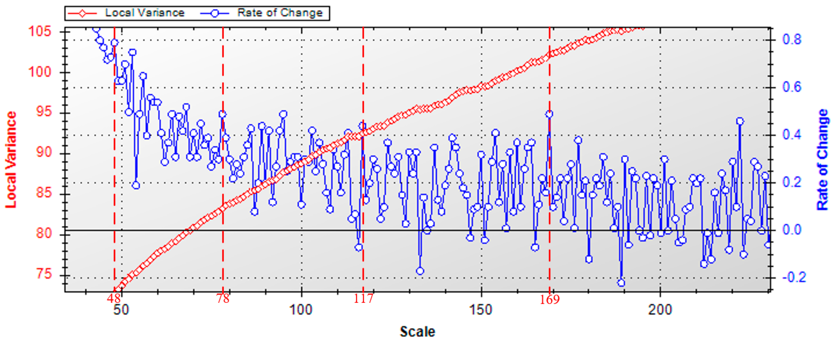
Bottom-up coarse fusion: Adjacent segments progressively merge, guided by tracking nodes along each path. Homogeneity analysis ensures merging stops when regions belong to the same geographic element, preventing excessively small objects with high internal variability. However, if an abrupt drop in LV accompanies object homogeneity, it indicates a potential small changed object within, triggering the corresponding node as optimal for that path.

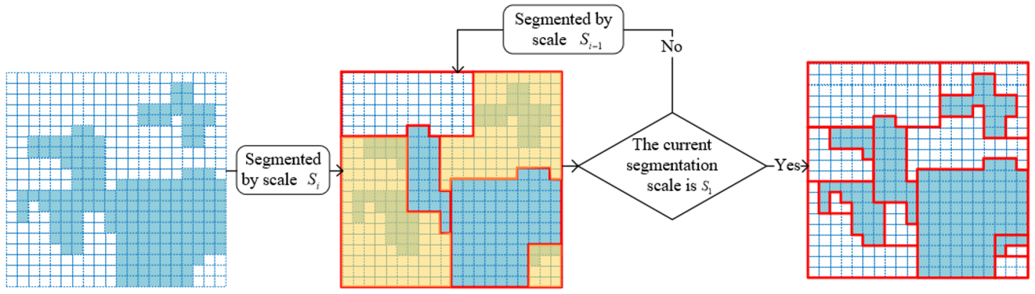
(2)

Top-down fine splitting: To generate objects that conform to the boundaries of actual changed ground objects minimizing segmentation omissions, the stacked $X^{t_1}$ and $X^{t_2}$ images are iteratively segmented based on the PBCD binary map, with CVA as a representative, as shown in Figure 3. Segmentation from the coarsest optimal node along each path and a top-down assessment determines participation in the next scale of segmentation until the finest scale is reached. In each iteration i with scale S_i, the objects derived from the previous iteration (scale S_i−1) undergo re-segmentation if proposition (1) is satisfied (yellow regions in Figure 3).

$$p:({\mu }_{\mathrm{CVA},j}\ne 0)\wedge ({\sigma }_{\mathrm{CVA},j}\ne 0)$$

(1)

where ${\mu }_{\mathrm{CVA},j}$ and ${\sigma }_{\mathrm{CVA},j}$ are the mean and standard deviation of the object patch $j$ in the CVA binary map, respectively. Hierarchical optimal segmentation results can be obtained by this iterative segmentation, which are tailored to real-world features of different sizes.

To quantitatively analyze the segmentation performance in change areas, the segmentation MIoU (mean intersection over union) is used as a metric [37].

$$MIoU=\left[\frac{TP}{TP+FP+FN}+\frac{TN}{TN+FP+FN}\right]/2$$

(2)

where MIoU is the metric commonly used to evaluate the performance of segmentation models, measuring the average intersection over union across binary classes. TF, TN, FP, and FN are parameters of the confusion matrix given in Section 2.4.

2.2. Feature Extraction and Optimization

2.2.1. Construction of Feature Space

Stacked remote sensing image objects can be characterized by a feature space constructed from spectral and texture features. In this space, objects with similar features are grouped into classes, which facilitates the extraction of change information.

Spectral features, which describe the spectral information of reflectance, are important for CD. Common spectral features include single-band gray mean, standard deviation, and spectral indices, such as the Normalized Difference Vegetation Index (NDVI) and the Normalized Difference Water Index (NDWI). The NDVI is sensitive to vegetation, while the NDWI is sensitive to water [38].

$$NDVI=(NIR-R)/(NIR+R)$$

(3)

$$NDWI=(G-NIR)/(G+NIR)$$

(4)

In both the GF-1 WFV and GF-6 WFV data, the variables R, G, B, and NIR represent the reflectance values corresponding to the red, green, blue, and near-infrared bands, respectively.

Texture features describe the spatial relationships between pixels in an image. The entropy value in the gray-level co-occurrence matrix (GLCM) is a commonly used texture feature that measures the uniformity of the texture. A smaller entropy value indicates a more uniform texture. In this study, we extracted eight commonly used texture features from the images using a sliding window of size 3 × 3 and a stride of 1, in four scan directions. The extracted texture features are listed in

Table 1. Statistics defined by GLCM.

Texture Feature	Formula	Texture Feature	Formula
GLCM_mean	${\displaystyle \sum _i{\displaystyle \sum _{j}i\cdot P(i,j)}}$	GLCM_dissimilarity	${\displaystyle \sum _i{\displaystyle \sum _j\left|i-j\right|P(i,j)}}$
GLCM_variance	${\displaystyle \sum _i{\displaystyle \sum _j{(i-u)}^{2}P(i,j)}}$	GLCM_entropy	$-{\displaystyle \sum _i{\displaystyle \sum _{j}P(i,j)}}\log P(i,j)$
GLCM_homogeneity	${\displaystyle \sum _i{\displaystyle \sum _{j}P(i,j)/[1+{(i-j)}^2]}}$	GLCM_ASM	${{\displaystyle \sum _i{\displaystyle \sum _{j}P(i,j)}}}^2$
GLCM_contrast	${\displaystyle \sum _i{\displaystyle \sum _{j}P(i,j)}}{(i-j)}^2$	GLCM_correlation	${\displaystyle \sum _i{\displaystyle \sum _j(i-{\mu }_x)(j-{\mu }_y)P(i,j)/{\sigma }_x{\sigma }_y}}$

Note: P is GLCM matrix, (i,j) is the index. ${\mu }_x$ and ${\mu }_y$ represent the mean values of row and column, respectively. ${\sigma }_x$ and ${\sigma }_y$ represent the standard deviation values of row and column, respectively.

[39].

2.2.2. Optimal Selection of Features

In theory, all features of remote sensing image objects should be used for CD. However, due to the “dimension disaster”, an excessive number of features impacts the processing efficiency and detection accuracy, especially when dealing with limited samples [8,40]. Therefore, it is important to optimize the useful features of CD. The Relief algorithm is widely used as the optimal selection method based on the concept of “Hypothesis-Margin”. The formula for updating the feature weights is as follows [41]:

$$W_f^i=W_f^{i-1}+{\displaystyle \sum _{c\ne class(x)}\frac{\frac{p(x)}{1-p(class(x))}{\displaystyle \sum _{j=1}^{k}dif{f}_f(x,M(x))}}{m\times k}}-{\displaystyle \sum _{j=1}^k\frac{dif{f}_f(x,H(x))}{m\times k}}$$

(5)

where $i$ represents random samples and $dif{f}_f()$ represents the distance of samples on feature $f$. $H(x)$ and $M(x)$ denote the nearest sample in the same and non-same class as $x$, respectively. $p()$ denotes class probability, $m$ denotes the iteration number, and $k$ denotes the number of nearest neighbor samples.

2.3. Object-Oriented Regularized IRMAD

2.3.1. Object-Based IRMAD

This paper proposes a novel object-oriented method based on the IRMAD algorithm, an unsupervised classification algorithm with a proven track record of success at the pixel level. This method builds upon the original MAD algorithm [42] by introducing an object-based iterative weighting strategy that utilizes canonical correlation analysis to obtain object weights during the convergence process.

To measure the change between two objects in bi-temporal multispectral satellite images with features, we can apply linear transformations with projection vectors a and b to the vectors of object features $X={\left[X_1 X_2 \cdots X_p\right]}^{\mathrm{T}}$ and $Y={\left[Y_1 Y_2 \cdots Y_q\right]}^{\mathrm{T}}$ (p and q are the numbers of the features, respectively). Note that the object features can consist of the mean reflectance of spectral bands and other statistics, such as variance and entropy, while pixel-based methods typically involve only the spectral reflectance.

Formula (6) establishes the relationship among variables and describes the canonical variables’ correlation coefficients in MAD results in an ascending order that is represented as:

$$\left[\begin{array}{l}\mathrm{MA}{\mathrm{D}}_1\\ \mathrm{MA}{\mathrm{D}}_2\\ ⋮\\ \mathrm{MA}{\mathrm{D}}_p\end{array}\right]=\left[\begin{array}{l}{a}_p^{T}X-b_p^{T}Y\\ a_{p-1}^{T}X-b_{p-1}^{T}Y\\ ⋮\\ a_1^{T}X-b_1^{T}Y\end{array}\right]$$

(6)

As the MAD variables are a linear combination of random variables X and Y, they approximately follow a normal distribution according to the central limit theorem. Therefore, the squared MAD variables divided by the sum of variances follow a chi-square distribution with p degrees of freedom:

$$T_j={{\displaystyle \sum _{i=1}^p(\frac{\mathrm{MA}{\mathrm{D}}_{ij}}{{\sigma }_{\mathrm{MAD}i}})}}^2\in {\kappa }^2\left(p\right)$$

(7)

where p represents the number of features and j represents the j-th object, respectively.

The iterative reweighting scheme assigns weights to the objects during the iteration process, where the weights of the objects below a threshold value $t\in [0,1]$ are extracted as changed objects.

Since the MAD variables follow a chi-square distribution as shown in Equation (7), the new weight $w^{\prime }$ for each object can be obtained using Formula (8). The quantile $\mathsf{\partial }$ represents the percentile point of the chi-square distribution.

$$w^{\prime }=1-\mathsf{\partial }$$

(8)

2.3.2. Regularized Canonical Correlation

In the standard MAD algorithm, the variance–covariance matrix of the original random variables can become nearly singular after multiple iterations, due to the over-reliance on noise or spurious differences in eigenvalue computations. To avoid this issue, a regularization term is introduced to mitigate the ill-posed nature of the generalized eigenvalue problem. The well-known Canonical Correlation Analysis (CCA) formula can be modified as follows:

$$\left[\begin{array}{l}0\\ {\sum }_{YX}\end{array}\begin{array}{r}{\sum }_{XY}\\ 0\end{array}\right]\left[\begin{array}{c}a\\ b\end{array}\right]=\rho \left[\begin{array}{cc}{\sum }_{XX}+{\lambda }_1{\mathsf{\Omega }}_1& 0\\ 0& {\sum }_{YY}+{\lambda }_2{\mathsf{\Omega }}_2\end{array}\right]\left[\begin{array}{c}a\\ b\end{array}\right]$$

(9)

where ${\sum }_{XY}$ and ${\sum }_{YX}$ are the covariance between $X$ and $Y$, and $\rho =Corr\left\{a^{T}X,b^{T}Y\right\}$ is the canonical correlation. The linear combinations of X and Y exhibiting maximum correlation can be found by identifying the optimal projection vectors $a$ and $b$. The penalization curvature ${\mathsf{\Omega }}_i$ is defined as the product of the transpose of the matrix L and L itself, i.e., $\mathsf{\Omega }=L^{T}L$, and ${\lambda }_i$ governs the extent of the penalty. The matrix L, typically chosen according to Formula (10), is a (p−2) × p matrix (typically p = q) that approximates the discrete second derivative. This regularization term serves to impose a penalty on the feature vectors, promoting smoother and more stable solutions by controlling the local curvature properties of a and b. $trace{\sum }_{XX}/trace{\mathsf{\Omega }}_1$ and $trace{\sum }_{YY}/trace{\mathsf{\Omega }}_2$ are assigned to ${\lambda }_1$ and ${\lambda }_2$, respectively, which can quantify the degree of penalization. Given that X and Y represent distinct but similar types of data in this study, ${\lambda }_1={\lambda }_2=\lambda$ and ${\mathsf{\Omega }}_1={\mathsf{\Omega }}_2=\mathsf{\Omega }$ are the hypotheses.

$$L=\left[\begin{array}{cccccc}1& -2& 1& 0& \cdots & 0\\ 0& 1& -2& 1& \cdots & 0\\ ⋮& ⋮& ⋮& \ddots & ⋮& ⋮\\ 0& 0& \cdots & 1& -2& 1\end{array}\right]$$

(10)

2.4. Accuracy Assessment

To assess and evaluate the accuracy of the proposed method, a sample set consisting of uniformly distributed target objects was selected. Confusion matrix was employed to calculate various performance metrics, including precision, recall, overall accuracy (OA), Kappa, and F-score [43]. The specific values in the confusion matrix are described in

Table 2. Confusion matrix of CD.

Detection Result Ground Truth	Unchanged	Changed	Total
Unchanged	TP	FN	NT
Changed	FP	TN	NF
Total	NP	NN	N

.

A higher precision indicates fewer false detections, while a higher recall indicates fewer missed detections. F-score is the harmonic mean of precision and recall, which provides a balanced measure of a model. OA measures the overall correctness of the model’s predictions, and Kappa considers the heterogeneity between the predicted results and random predictions.

3. Results

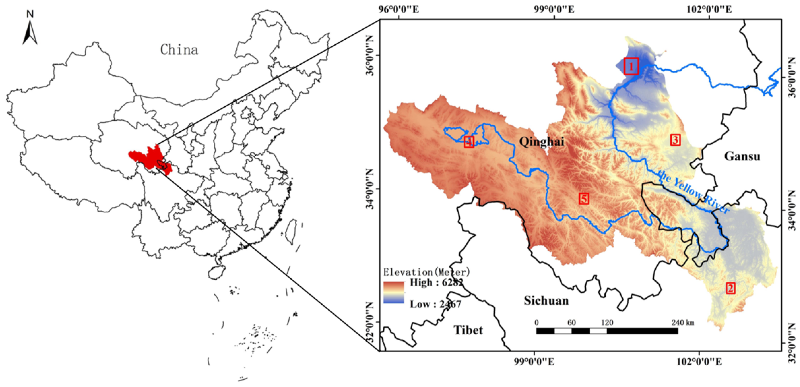
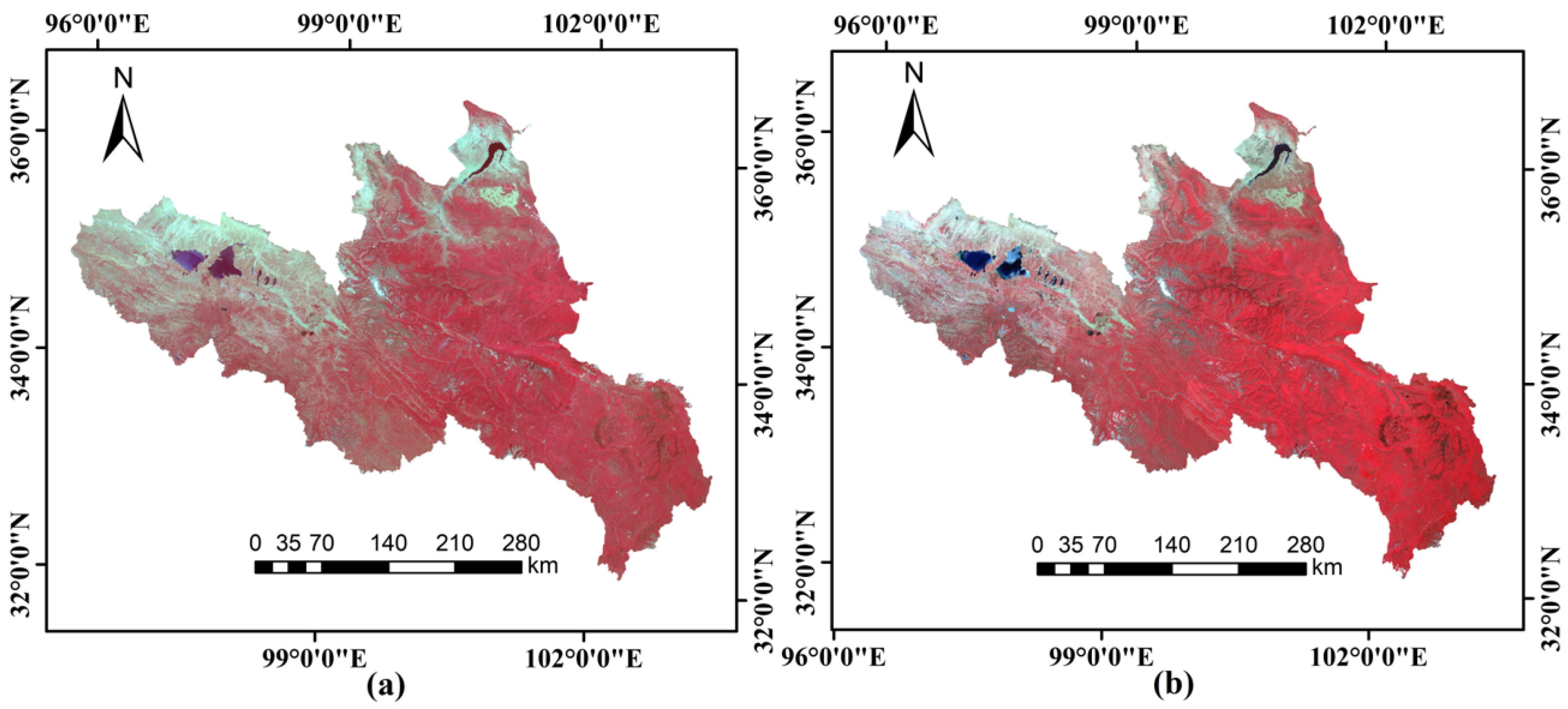
3.1. Study Area and Data Preprocessing

The Yellow River source region (YRSR) is located in the northeast of the Qinghai-Tibet Plateau. It is the birthplace of the Yellow River and a significant part of the Three-River Source Region, the largest water supply and functional conservation area in China [44]. This region includes seven ecosystems including grasslands, wetlands, build-up areas, forests, scrub, deserts, and glacier, covering a total area of 131,667.58 km². However, the ecosystems in the YRSR are highly sensitive to environmental changes due to the high altitude and complex topography [45]. In recent years, the climate in the source region has exhibited a trend from cold-dry to warm-humid, while this region exhibits rich human production and life activity as well as a series of government protection measures. There have been significant changes in the land cover types of the various ecosystems in the YRSR. To better compare and demonstrate the changes, five subsets composed of representative features from the study area were selected for regional experiments (Figure 4). Among them, Subset 1 primarily focuses on the increase in photovoltaic land and the decrease in grassland. Subsets 2 and 3 mainly address changes in built-up areas and wetlands in Zekog County and Hongyuan County, which are important developing cities in the YRSR. Subset 4 considers changes in wetlands and grasslands around Nogring Hu. Subset 5 focuses on the degradation of vegetation in the vicinity of Gande County and the increase in bare land. The subsets are evenly distributed across various elevations in the study area, covering changes in various ecosystems.

This experiment utilized dual-temporal images from the GaoFen-1 (GF-1) and GaoFen-6 (GF-6) Wide Field of View (WFV) satellites, which are effective medium-resolution data sources for monitoring dynamic changes in the land surface cover [46]. The specific technical specifications of the satellites are shown in

Table 3. Technical specifications of sensors’ payload for GF-1 and GF-6.

Sensor	Spatial Resolution (m)	Width (km)	Band Name	Wavelength (μm)	Band Name	Wavelength (μm)
GF-1 WFV	16	800	B1 (blue)	0.45–0.52
			B2 (green)	0.52–0.59
			B3 (red)	0.63–0.69
			B4 (near-infrared)	0.77–0.89
GF-6 WFV	16	800	B7 (purple)	0.40–0.45	B3 (red)	0.63–0.69
			B1 (blue)	0.45–0.52	B5 (red-edge1)	0.69–0.73
			B2 (green)	0.52–0.59	B6 (red-edge2)	0.73–0.77
			B8 (yellow)	0.59–0.63	B4 (near-infrared)	0.77–0.79

. The multi-spectral image data were provided by the China Center for Resource Satellite Data and Application (CRESDA, http://www.cresda.com/). Selected images covering the study area were orthorectified using the RPC model and ground control points referenced to the Sentinel-2 Level-2A product and the SRTM DEM (30 m resolution). Subsequently, absolute radiometric and atmospheric corrections were performed using the coefficients provided by the CRESDA and the Second Simulation of the Satellite Signal in the Solar Spectrum (6S) model with MODIS atmospheric data. Bands B1-B4 of the two satellites were used for layer stacking, de-clouding, and image mosaicking to obtain the images of the YRSR shown in Figure 5. The details of used images are shown in

Table 4. Detailed information of GF images covering the study area.

Data	Imaging Time	Data	Imaging Time	Data	Imaging Time
GF1-WFV1	28 July 2015	GF1-WFV2	14 August 2015	GF1-WFV4	9 July 2015
	1 August 2015		6 July 2022		23 August 2015
	13 August 2015	GF1-WFV3	5 June 2015		29 July 2015
	23 August 2022		23 August 2015		22 July 2022
	29 July 2022		27 August 2015		6 July 2022
GF1-WFV2	28 July 2015		6 July 2022	GF6-WFV	25 July 2022
	1 August 2015		22 July 2022		8 July 2022
	5 August 2015	GF1-WFV4	25 July 2015		21 August 2022
	7 August 2022		29 July 2015

.

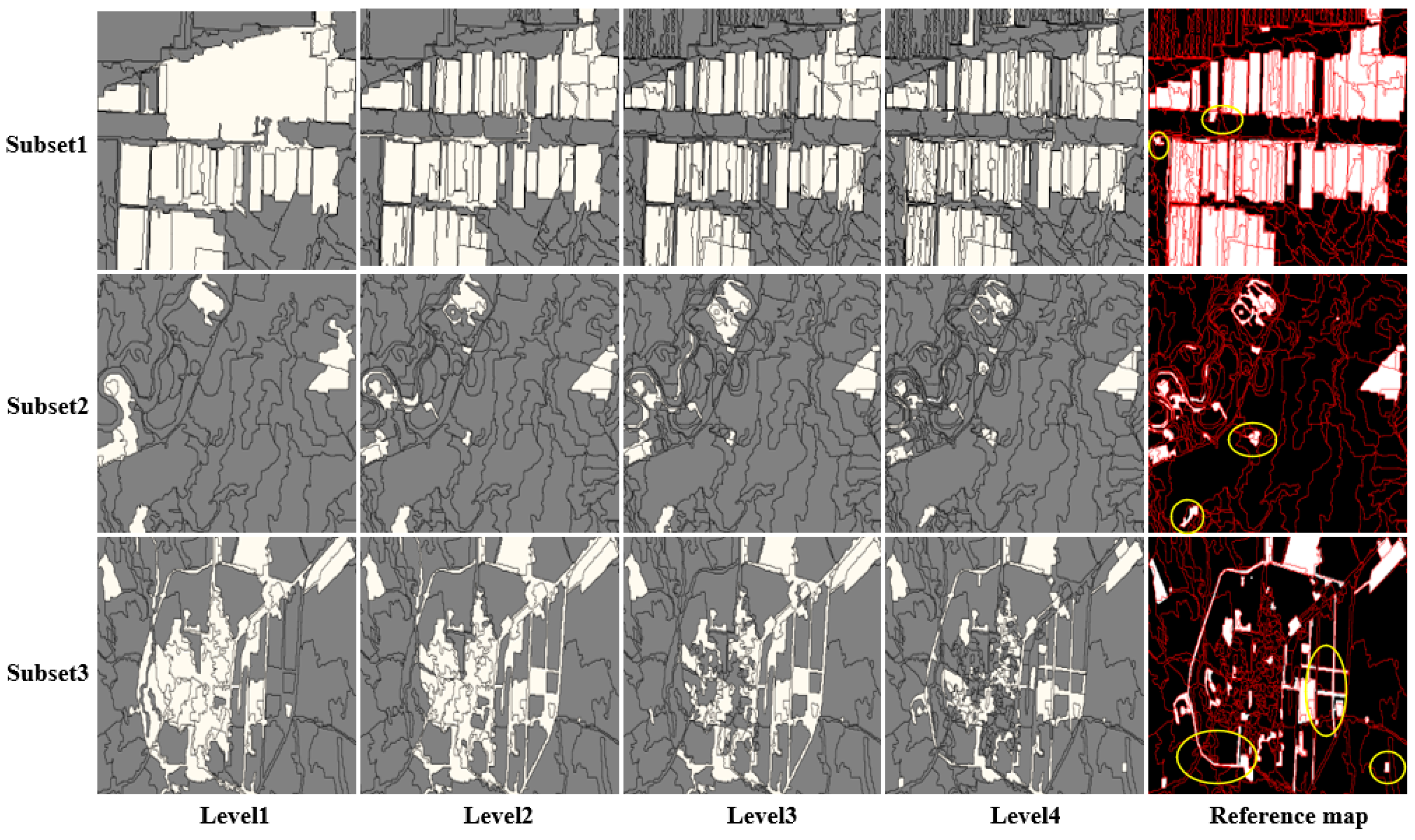
3.2. Results of Hierarchical Multi-Scale Segmentation

To generate object patches corresponding to the actual changed ground objects, ROC-LV, seen in Figure 6, is used to select the optimal segmentation scales. The scale corresponding to the peak value of ROC-LV on the red dashed line is an optimal segmentation scale. Multiple optimal segmentation scales can be obtained for different land cover types [36].

The stacked bi-temporal images were used as the basis for segmentation. Four scales corresponding to the peaks of 169, 117, 78 and 48 were chosen as the base scales for subsequent iteration levels. The shape factor and compactness factor were set to 0.4 and 0.5, respectively, based on experience.

Hierarchical multi-scale segmentation sequentially segments stacked images from coarse to fine scales, leveraging the PBCD-derived difference map statistics of objects at each scale to determine whether further segmentation is required. The local zoomed-in segmentation effects of the objects in each layer are shown in Figure 7, where the gray area represents the unchanged detection results and the white area represents the changes. At a segmentation scale of 169, “under-segmentation” is evident, especially for objects like white buildings and roads, which occupy relatively fewer pixels. As the image scale decreases, the pixel-based results provide an initial screening of potentially changing patches and gradually separate small objects (in yellow circles). Simultaneously, larger areas inherit the scale of the parent levels, preserving large scales suitable for unchanged objects. The objects generated by iterative scale segmentation are more compatible with the contours of the actual changed features. The MIoU and F-score in

Table 5. The segmentation errors of different hierarchy levels.

		Subset 1	Subset 2	Subset 3
Level 1	MIoU	0.7757	0.6828	0.5259
	F-score	0.8717	0.9729	0.8619
Level 2	MIoU	0.9097	0.8401	0.5405
	F-score	0.9562	0.9892	0.8688
Level 3	MIoU	0.9273	0.8244	0.5847
	F-score	0.9662	0.9874	0.8984
Level 4	MIoU	0.9456	0.9316	0.7154
	F-score	0.9739	0.9962	0.9482

increase as the hierarchy levels increase, indicating more efficient and accurate segmentation.

3.3. Feature Analysis and Optimization

In the experiment, the Relief method was used to optimize the 42 features (including 8 original spectral statistics of satellite images, 2 spectral indexes, and 32 texture features), and the importance of the features was sorted from the feature weights (as shown in Figure 8). The mean and standard deviation of the fourth band (MeanB4 and StdB4) contributed significantly to CD, with importance weights of 0.21 and 0.19, respectively. Among the texture indices, entropy and correlation from four bands ranked prominently in terms of importance, while the spectral indices NDVI and NDWI also played significant roles.

Based on the order of feature importance, the features were sequentially selected in the CD process, resulting in the curve shown in Figure 9. As illustrated in the figure, with the increase in the feature number participating in CD, the overall accuracy of the test samples in each subset shows an “increase-steady-decline” trend, indicating that increasing features lack monotonically positive effects on CD accuracy. To balance the performance over a wide range, we selected 11 features that performed well in all five subsets, so that the optimal feature space was constructed, as indicated by the red box in Figure 8. These 11 features include 4 spectral statistics, 2 spectral indices, and 5 texture indices.

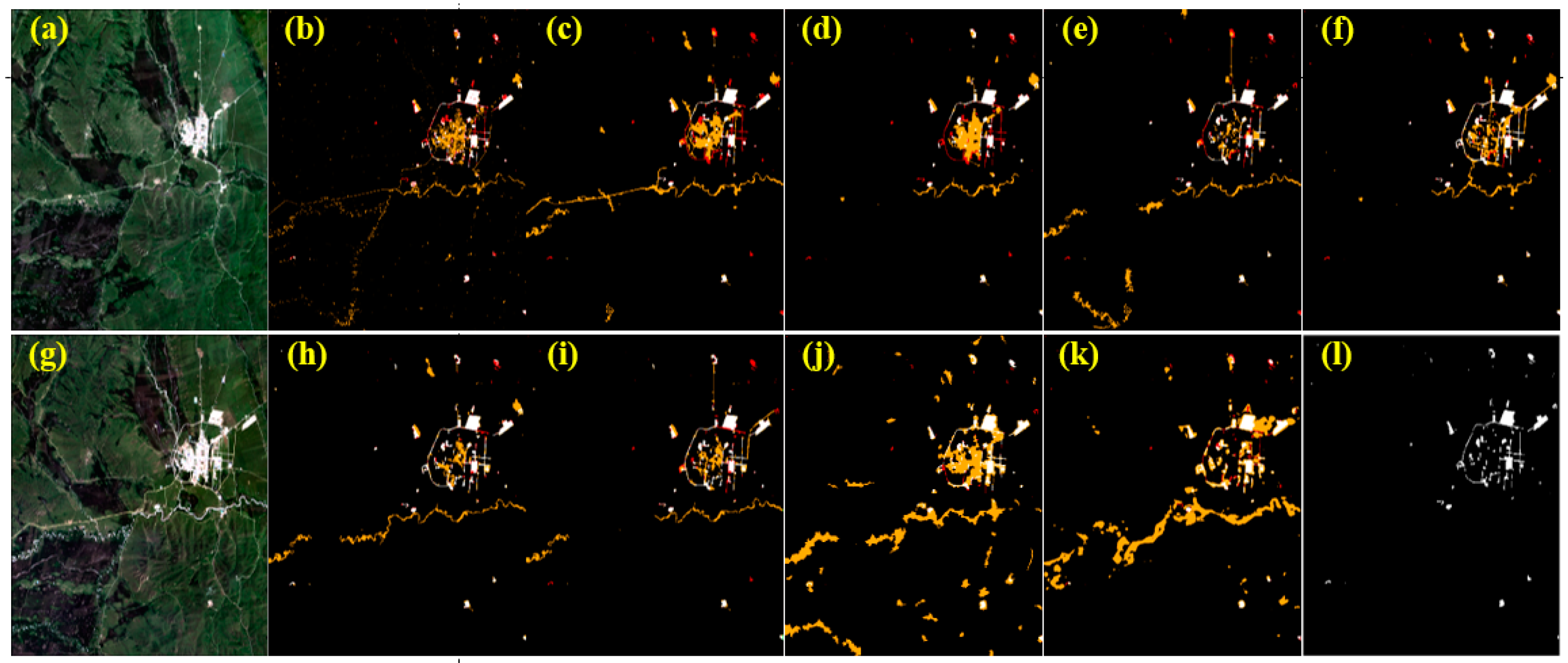
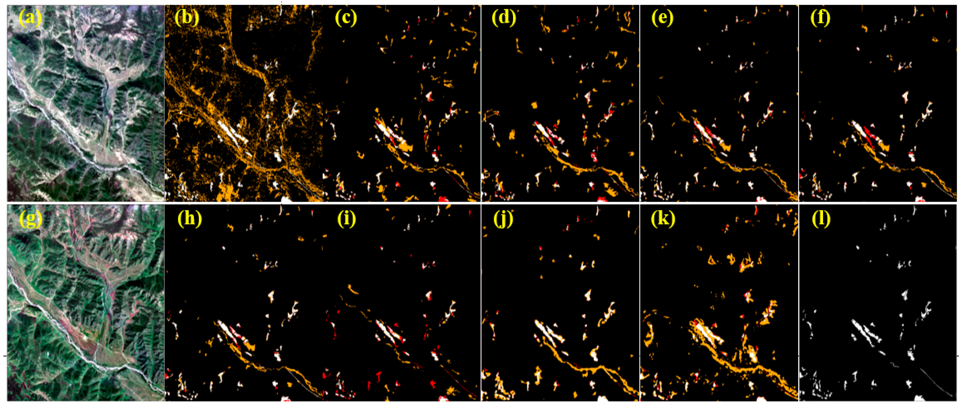
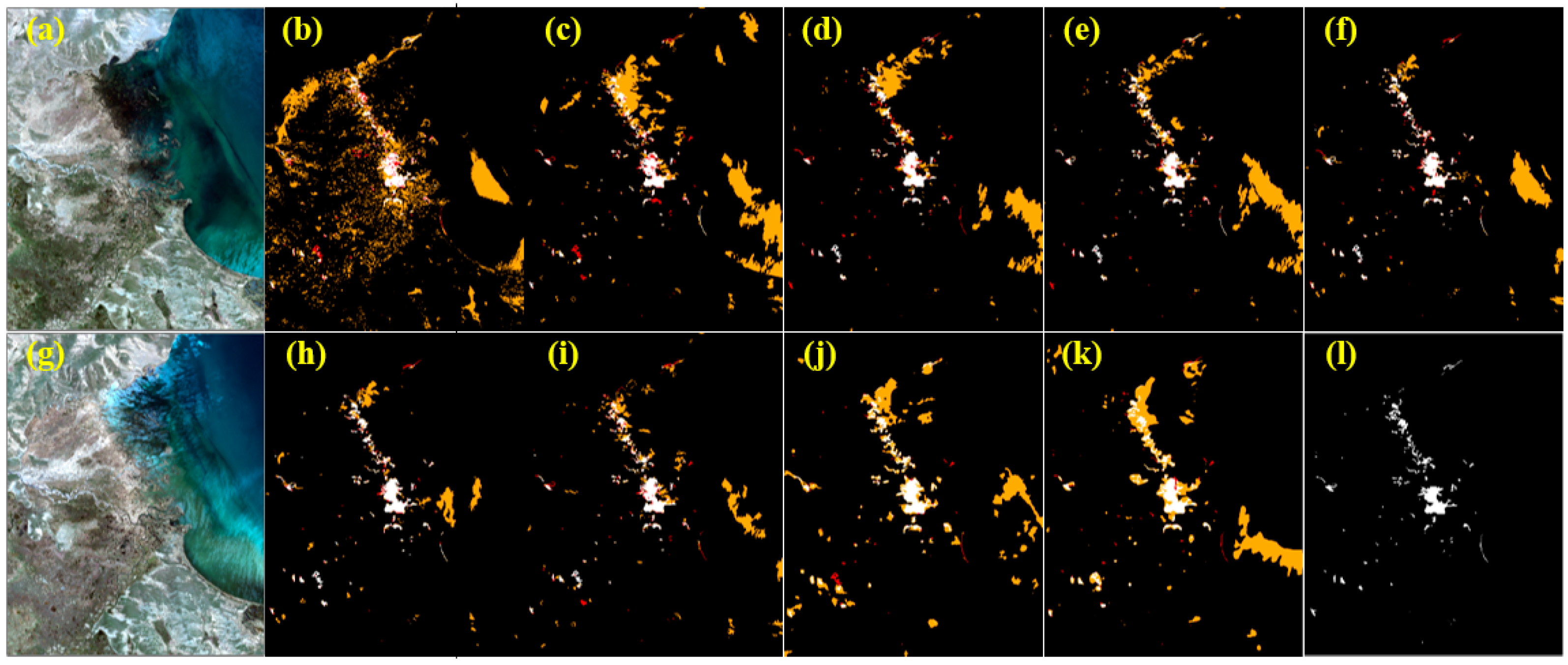
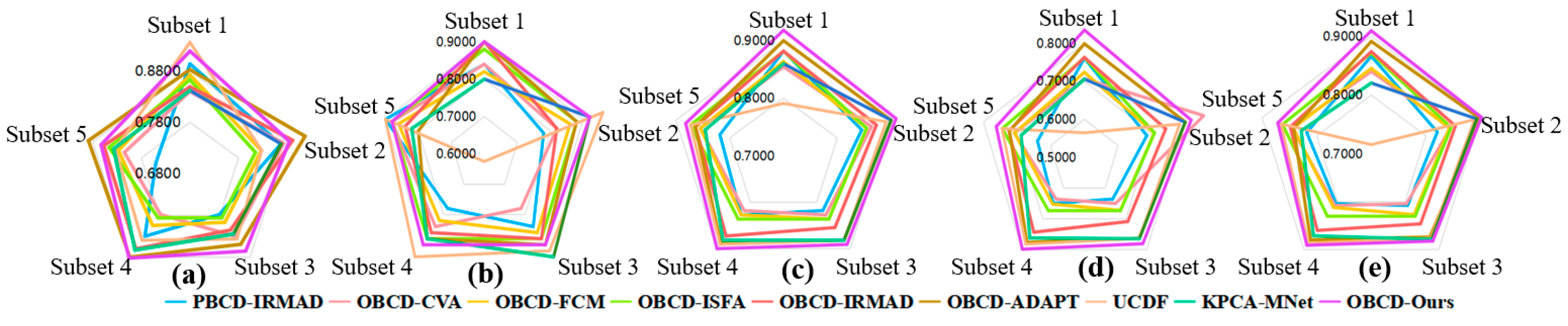
3.4. OBCD Experiments

To evaluate the effects of the improved OBCD-IRMAD used in the proposed object-oriented changed detection approach, we designed comparative experiments in five subsets of representative changes. As comparisons, we conducted experiments with eight approaches, including pixel-level, object feature-level, object decision-level and deep learning approaches, namely, PBCD-IRMAD [47], OBCD-CVA [48], OBCD-FCM [49], OBCD-ISFA [50], OBCD-IRMAD [22], OBCD-DST [27], KPCA-MNet [51], and UCDF [30], and compared the results in conjunction with the change reference map drawn from visual interpretation.

Figure 10, Figure 11, Figure 12, Figure 13 and Figure 14 visualize the binary change maps for different methods. Black pixels represent true positives (TPs), orange represents false negatives (FNs), red represents false positives (FPs), and white represents true negatives (TNs). Overall, our approach demonstrates effective CD results, maintaining a low level and harmonious balance both FN and FP.

Qualitatively, PBCD-IRMAD methods often struggle with noise rejection due to limitations in spatial resolution, but they successfully detect most changes. By transitioning from PBCD to object-level, our approach leverages larger-scale basic units to effectively mitigate the impact of noise on the results. This performance improvement is evidenced in

Table 6. The average assessments of CD in five subsets.

	PBCD- IRMAD [47]	OBCD-CVA [48]	OBCD-FCM [49]	OBCD-ISFA [50]	OBCD- IRMAD [22]	OBCD-DST [27]	UCDF [30]	KPCA-MNet [51]	Improved OBCD-IRMAD
precision	0.8236	0.8269	0.8253	0.8190	0.8545	0.8834	0.8544	0.8468	0.8827
recall	0.8280	0.8320	0.8440	0.8800	0.8600	0.8720	0.8600	0.8720	0.9000
OA	83.82%	84.36%	84.73%	85.64%	86.91%	88.69%	86.55%	87.38%	90.00%
Kappa	0.6742	0.7111	0.6927	0.7123	0.7362	0.7722	0.7277	0.7439	0.7987
F-score	0.8234	0.8287	0.8341	0.8481	0.8565	0.8770	0.8467	0.8584	0.8912

, with the average assessment of five subsets, where both OA and F-score of PBCD-IRMAD are lower than the mean values. Notably, the addition of regularization contributes to robust iterations with multiple features. Compared to other feature-level methods, the improved OBCD-IRMAD exhibits superior performance, which adapts well to the specific features of WFV imagery.

In Figure 10, Figure 11, Figure 12, Figure 13 and Figure 14, subfigure (i) demonstrates the decision-level fusion of multiple PBCD results, effectively suppressing the salt-and-pepper noise. However, OBCD-DST has the highest precision but underperforms in average recall in Table 6. This multi-algorithm approach, relying solely on spectral features, can overlook subtle changes due to its limited information intake. Our approach maximizes the use of spectral and texture features to construct an optimal feature subset, ensuring a higher recall while minimizing false detection.

In contrast, the deep learning methods in subfigures (j) to (k) excel at identifying major changes through the analysis of high-level features. They are not only sensitive to changes in wetland ecosystems but also capable of mitigating false detections caused by imaging style differences. Although explicit segmentation is optional for end-to-end learning, slight variations in unsupervised classification hyperparameters can lead to disparate pixel outcomes, causing circular misclassifications and omissions at change boundaries. The segmentation method proposed in our study closely aligns with actual object boundaries, yielding superior F-scores. Compared to deep learning methods, the inclusion of feature selection alleviates the computational burden of CD, enabling larger-scale applications.

Figure 15 displays assessment radar charts for each subset, where our approach, in comparison to others, demonstrates a better balance in application capability, with Kappa and F-scores closer to the outer edge. This is further corroborated by the average quantitative assessments in Table 6, which demonstrates that the improved OBCD-IRMAD more effectively identifies the change objects with an OA of 90.00% and maintains a balanced relationship between precision and recall. The average F-score of 0.8912 demonstrates the superiority of the improved OBCD-IRMAD method, surpassing all other methods.

Taking the results from all five subsets into account (Figure 15), the improved OBCD-IRMAD method demonstrates superior sensitivity in distinguishing construction land and vegetation, especially in areas with significant spectral and textural differences. It attains the peak F-score in subset 1, showcasing robust detection capabilities, especially in discerning changes of photovoltaic land and grassland. In subsets 1, 2, and 3, which encompass regions with diverse altitudes and changes in land cover ecosystems, the recall values consistently surpass 90%, underscoring strong capacities for CD with actual changes. However, for subsets 4 and 5, which are characterized by wetland, grassland, and bare land, the improved OBCD-IRMAD exhibits some false detection. Nevertheless, compared to other methods, it consistently outperforms in terms of OA, Kappa, and F-score.

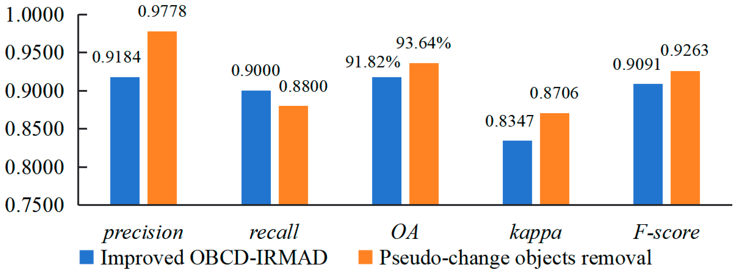
3.5. Ablation Experiments

To evaluate the individual contributions of our improved modules to OBCD-IRMAD performance in binary change detection, we conducted ablation experiments focusing on three key variables: improved OBCD-IRMAD (with regulation), hierarchy iterative segmentation of objects (HIS), and feature optimization (FO). The quantitative results are demonstrated in

Table 7. Quantitative analysis of ablation experiments on subset 3.

	Improved-IRMAD	HIS	FO	Precision	Recall	F-Score
OBCD-IRMAD				0.8148	0.8800	0.8462
Improved OBCD-IRMAD	√			0.8776	0.8600	0.8687
Improved OBCD-IRMAD+HIS	√	√		0.8627	0.8800	0.8713
Improved OBCD-IRMAD+FO	√		√	0.8491	0.9000	0.8738
Improved OBCD-IRMAD+HIS+FO	√	√	√	0.8654	0.9000	0.8824

.

According to Table 7, the integration of three strategic modules significantly enhanced the performance of our object-based change detection method, OBCD-IRMAD.

Regularization: Increased stability, leading to an F-score of 0.8687.

HIS: Refined object boundaries and details, mitigating omission detections and further increasing F-score.

FO: Focused OBCD on the most informative features, elevating F-score to 0.8738. While this boosted recall and unsupervised clustering capabilities, it also introduced more false positives.

Combined integration: Strategically integrating these modules yielded a remarkable improvement in overall F-score from 0.8462 to 0.8824, demonstrating a more balanced treatment of object-specific discriminative features.

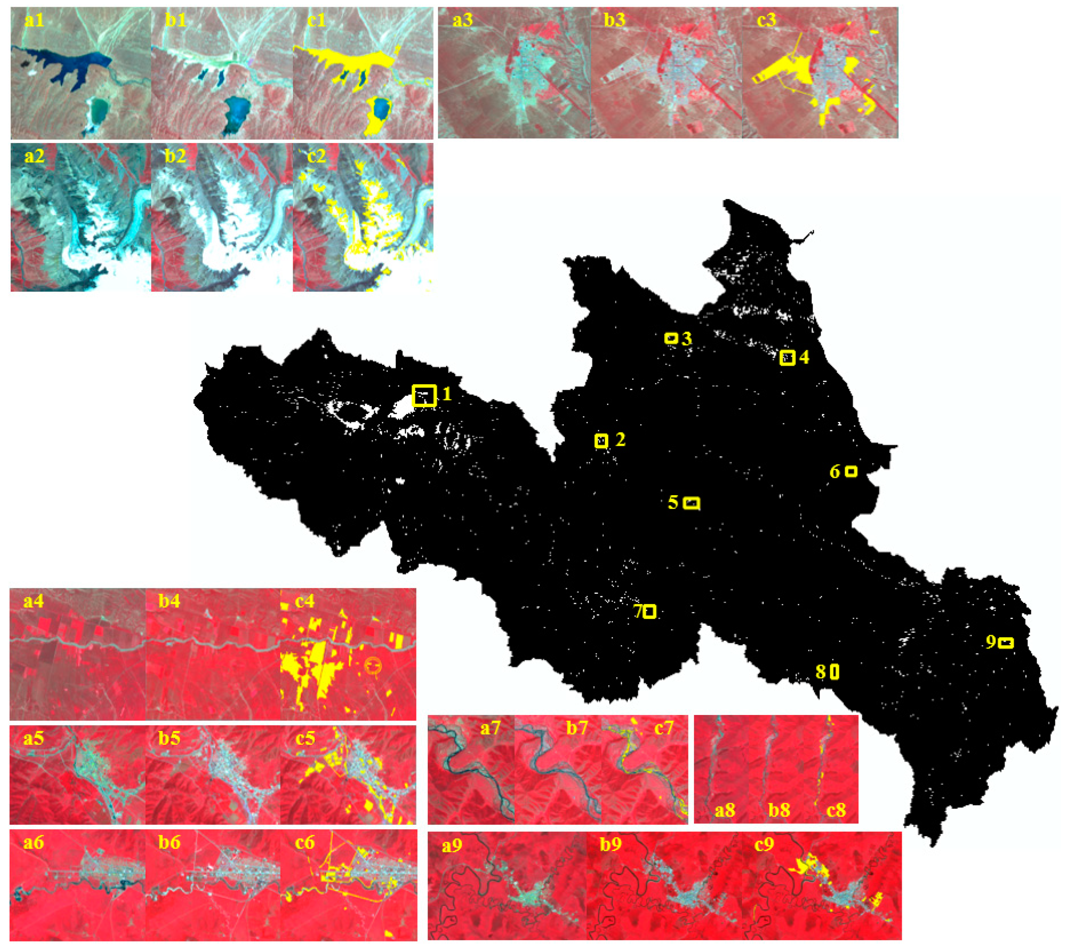
3.6. A Case Study in the Yellow River Source Region

Following the integrated approach described earlier, the images of the entire YRSR for 2015 and 2022 underwent hierarchical iterative segmentation at multiple scales, and 11 optimized features were inputted into the improved OBCD-IRMAD method, resulting in the binary change map and local zoomed-in maps displayed in Figure 16. The local zoomed-in maps use false color (R: B4, G: B3, B: B2) images as base maps, with detected changes highlighted in yellow. A total of 2120 validation samples were established, consisting of 900 samples in the changed area and 1220 samples in the unchanged area. These samples were evenly distributed across various ecosystems in the YRSR. Calculated according to the formulas, the OA, Kappa, and F-score of the whole study area are 90.09%, 0.7977 and 0.8844, which can meet the application requirements of ecosystem CD in the YRSR. The proposed hierarchical multi-scale segmentation object-oriented CD approach has applicability to the large-scale range of the WFV images. During the period from 2015 to 2022, the ecosystems in the YRSR experienced changes covering 1864.98 km², approximately 1.42% of the total area. Figure 16 reveals that these changes have occurred mainly in the northern and southeastern regions of the YRSR, including grassland, wetland, artificial ecosystems, as well as major urban areas.

The proposed approach exhibits relatively few omission errors in the entire study area, with a recall of 0.8922. However, there are some cases of false detections, with a precision of 0.8766. The relatively high proportion of omission detections occurs in grassland and wetland ecosystems, primarily due to the main features of vegetation cover reduction in the natural degradation process of these ecosystems. This implies that minor changes occur in the regions, making it difficult to distinguish because of similar features in the two temporal phases.

Figure 16 and

Table 8. Sample analysis for omission and false detection in the Yellow River Source.

Primary Ecosystems	Forest	Scrub	Grassland	Wetland	Artificial	Desert	Glacier
Number of changed samples	110	126	160	160	160	144	40
Number of unchanged samples	200	200	200	200	200	176	44
Number of omission detections	3	2	27	23	22	17	3
Number of false detections	5	3	24	27	32	19	3
Percentage of omission detections among all changed samples	2.73%	1.59%	16.88%	14.38%	13.75%	11.81%	7.50%
Percentage of false detections among all unchanged samples	2.50%	1.50%	12.00%	13.50%	16.00%	10.80%	6.82%

reveal that false detections are primarily observed in certain farmlands of the artificial ecosystem (depicted in Figure 16(c4)) and in the rivers and lakes of the wetland ecosystem shown in Figure 16(c1). These false detections account for 16.00% and 13.50% of the total each. When expanding the CD in the whole YRSR, the false percentage of false detections among all changed samples became higher than that in the subsets. This increase is primarily attributed to changes occurring in the agricultural land within the artificial ecosystem and water bodies within the wetland ecosystem. The vegetation types in farmland depend on human cultivation activities, and changes in rivers and lakes are often influenced by cloud and snow cover, making these changes typically not considered as genuine changes of the land cover ecosystems.

Ecosystem changes significantly impact the delivery of high-value services. The continuous promotion of ecological governance in the YRSR, supported by local policies and remote sensing detection, is essential for fostering high-quality development in the region [52]. Our integrated object-oriented CD approach generates binary change maps, pinpointing ecosystem changes over a large area, laying a solid foundation for semantic change discernment. This technology also allows timely focus on localized area of degradation for developing localized solutions.

4. Discussion

The results of OBCD are often contingent on the quality of segmentation, making it challenging to determine the optimal segmentation parameters. The identification of changes in ecosystems is complicated due to their varied sizes and diverse boundaries. With the enhancement of both spectral and spatial resolution in imagery, the heightened information content in the images presents fresh hurdles, including the detection of comparatively subtle changes and navigating the intricacies arising from diverse features. The feature optimization and the improved IRMAD algorithm proposed in this paper can overcome those hurdles, making the detection results more accurate and reliable. To better apply the CD approach in practical situations, it is necessary to discuss the following issue.

Even after accurate radiometric correction, unchanged ground features will typically exhibit some differences in satellite remote sensing images in the pre- and post-phases. For example, differences in surface conditions such as soil moisture, vegetation phenology, and crop cultivation within the same range at different time periods can lead to variations in spectral reflection characteristics and texture states of ground objects in the images, resulting in “false changes”. This problem is prevalent in CD methods [53,54], and it is also present in experiments of the improved OBCD-IRMAD, especially in subset 1. When applied to the case of the YRSR, a border scope of research involves the stitching of more images, which are usually acquired under different conditions, including varying solar angles and humidity environments.

Consequently, it is susceptible to limitations in recall and precision imposed by imaging conditions. Previous studies have made some attempts to address the causes of false changes, such as by using eco-geographical zoning data and crowdsourcing in WFV images [55]; the topographically controlled subpixel-based change detection model reduces the false detection over rugged terrain region [56]; and so on. To reduce this effect, the idea of unsupervised classification and further using the Iterative Self-Organizing Data Analysis Techniques Algorithm (ISODATA) method to cluster the changed objects [57] were introduced.

The changed objects were clustered into 10 categories (as shown in Figure 17), each of which reflects similarity in certain spectral or textural features. Grasslands in regions 1, 2, and 4 were practically unchanged, but their spectral characteristics differ due to various environmental factors. According to the clustering results, this region could be extracted by categories 4 and 6, and the pseudo-changes can be removed. Similarly, the pseudo-changes with different imaging times in cropland in region 3 and water in region 5 can be removed by category 8 and category 5. This method extracts and eliminates most of the pseudo-change regions with representative features in automatic detection, increasing the precision value by 0.0594 and the OA to 93.64% (Figure 18). However, it also removes some of the real changed objects, reducing the recall value by 0.0200.

Our proposed approach demonstrates considerable success in change detection, but further work is necessary to reduce the occurrence of pseudo-changes. Further experiments and optimization are still needed in terms of setting the hyper-parameters and improving post-processing methods. Similarly, constraints based on expert knowledge and preliminary research can be incorporated into the CD strategy. Additionally, by integrating Synthetic Aperture Radar (SAR) and higher-resolution remote sensing imagery, the technological pathways for leveraging multi-source data can be explored to detect more change information, thereby expanding the data sources and observational perspectives for change detection.

To further refine change detection results, we will explore the application of supervised classification techniques within identified changed objects. Random forests and support vector machines hold promise for accurately identifying specific “from-to” changes, thereby mitigating pseudo-changes arising from differing imaging conditions. By binarizing changes and describing them in semantic understanding, alterations in the ecosystem are identified. This method enables local communities to swiftly address ecosystem degradation and provides scientific support for regional ecological conservation.

5. Conclusions

In this paper, we applied an integrated object-oriented CD approach and conducted thorough experiments on GaoFen WFV imagery. In this approach, we (1) iteratively segmented images by the bi-directional segmentation strategy utilizing the BPT model with the PBCD difference map to derive multi-scale objects that are appropriate for the genuine change sizes and (2) optimized spectral and texture features of objects to align with the multidimensional features of the improved OBCD-IRMAD method.

In comparison with advanced unsupervised methods, our improved OBCD-IRAMD method presents better performance, which is more adapted for the selected 11 features in WFV. The proposed hierarchical multi-scale segmentation method accurately delineates the boundaries of changed objects, particularly small-scale objects. Increasing the number of object features involved in CD does not necessarily lead to a linear boost in OA. However, through feature selection and optimized space construction, the issue of dimensionality explosion can be mitigated. Experiments have demonstrated the feasibility and effectiveness of the approach for improving the accuracy of CD. In addition, the successful application in the YRSR has also shown that there are significant localized ecosystem changes in the YRSR in 2015–2022, with the changed area accounting for about 1.42% of the whole YRSR. These changes mainly occur in the grassland, wetland, and artificial ecosystems in the northern and southwestern parts of the source area. The integrated approach has an OA of 90.09% and an F-score of 0.8844 in the entire resource.

Our primary contribution is the introduction of an object-oriented unsupervised CD approach based on bi-directional hierarchical multi-scale segmentation strategy and ful optimization of high-dimensional features. The integrated approach overcomes the common pitfalls of underutilized features and high dimensionality in binary CD for GaoFen WFV imagery and creates a richer feature space encompassing spectral statics, indices, and texture information. The method achieves a balance in detecting objects of varying sizes across large-scale study areas, especially subtle changes. All contributions pave the way for significantly improved accuracy and efficiency of large-scale regional approaches in CD tasks, which is important for understanding and monitoring land ecosystem changes and promoting human–land harmony.

The practice case of our integrated approach in the YRSR reveals the locations of ecosystem changes in the vital water conservation area of the Yellow River basin. It contributes to precise ecosystem restoration and protection, enhancing ecological service capabilities. The findings provide scientific evidence for ecological conservation and sustainable management in the Yellow River basin, offering robust decision support for local governments and ecological conservation organizations.

However, since environmental factors such as vegetation phenology and imaging conditions can lead to spurious changes in non-target areas, the proposed method may be susceptible to such changes, potentially affecting the OA. Consequently, we will devote our future research on correcting errors on the basis of ensuring the precision of the CD.

References

1. Hussain, M.; Chen, D.; Cheng, A.; Wei, H.; Stanley, D. Change detection from remotely sensed images: From pixel-based to object-based approaches. ISPRS J. Photogramm. Remote Sens. 2013, 80, 91–106. [Google Scholar] [CrossRef]
2. Diaz-Delgado, R.; Cazacu, C.; Adamescu, M. Rapid Assessment of Ecological Integrity for LTER Wetland Sites by Using UAV Multispectral Mapping. Drones 2019, 3, 3. [Google Scholar] [CrossRef]
3. Sajjad, A.; Lu, J.Z.; Chen, X.L.; Chisenga, C.; Saleem, N.; Hassan, H. Operational Monitoring and Damage Assessment of Riverine Flood-2014 in the Lower Chenab Plain, Punjab, Pakistan, Using Remote Sensing and GIS Techniques. Remote Sens. 2020, 12, 714. [Google Scholar] [CrossRef]
4. Wang, H.B.; Gong, X.S.; Wang, B.B.; Deng, C.; Cao, Q. Urban development analysis using built-up area maps based on multiple high-resolution satellite data. Int. J. Appl. Earth Obs. Geoinf. 2021, 103, 17. [Google Scholar] [CrossRef]
5. Panuju, D.R.; Paull, D.J.; Trisasongko, B.H. Combining Binary and Post-Classification Change Analysis of Augmented ALOS Backscatter for Identifying Subtle Land Cover Changes. Remote Sens. 2019, 11, 100. [Google Scholar] [CrossRef]
6. Niemeyer, I.; Marpu, P.R.; Nussbaum, S. Change Detection Using the Object Features. In Proceedings of the IEEE International Geoscience and Remote Sensing Symposium (IGARSS), Barcelona, Spain, 23–27 July 2007; IEEE: Barcelona, Spain, 2007; p. 2374. [Google Scholar]
7. Hirayama, H.; Sharma, R.C.; Tomita, M.; Hara, K. Evaluating multiple classifier system for the reduction of salt-and-pepper noise in the classification of very-high-resolution satellite images. Int. J. Remote Sens. 2019, 40, 2542–2557. [Google Scholar] [CrossRef]
8. Blaschke, T. Object based image analysis for remote sensing. ISPRS J. Photogramm. Remote Sens. 2010, 65, 2–16. [Google Scholar] [CrossRef]
9. Wang, Z.; Wei, C.; Liu, X.; Zhu, L.; Yang, Q.; Wang, Q.; Zhang, Q.; Meng, Y. Object-based change detection for vegetation disturbance and recovery using Landsat time series. GIScience Remote Sens. 2022, 59, 1706–1721. [Google Scholar] [CrossRef]
10. Wang, J.; Jiang, L.L.; Qi, Q.W.; Wang, Y.J. Exploration of Semantic Geo-Object Recognition Based on the Scale Parameter Optimization Method for Remote Sensing Images. Isprs Int. J. Geo. Inf. 2021, 10, 420. [Google Scholar] [CrossRef]
11. Zhang, X.L.; Xiao, P.F.; Feng, X.Z.; Yuan, M. Separate segmentation of multi-temporal high-resolution remote sensing images for object-based change detection in urban area. Remote Sens. Environ. 2017, 201, 243–255. [Google Scholar] [CrossRef]
12. Xu, L.; Ming, D.; Zhou, W.; Bao, H.; Chen, Y.; Ling, X. Farmland Extraction from High Spatial Resolution Remote Sensing Images Based on Stratified Scale Pre-Estimation. Remote Sens. 2019, 11, 108. [Google Scholar] [CrossRef]
13. Xiao, T.; Wan, Y.; Chen, J.; Shi, W.; Qin, J.; Li, D. Multiresolution-Based Rough Fuzzy Possibilistic C-Means Clustering Method for Land Cover Change Detection. IEEE J. Sel. Top. Appl. Earth Obs. Remote Sens. 2023, 16, 570–580. [Google Scholar] [CrossRef]
14. Su, T.F. Scale-variable region-merging for high resolution remote sensing image segmentation. ISPRS J. Photogramm. Remote Sens. 2019, 147, 319–334. [Google Scholar] [CrossRef]
15. Zhang, X.L.; Xiao, P.F.; Feng, X.Z. Object-specific optimization of hierarchical multiscale segmentations for high-spatial resolution remote sensing images. ISPRS J. Photogramm. Remote Sens. 2020, 159, 308–321. [Google Scholar] [CrossRef]
16. Wang, Z.; Zhang, S.W.; Zhang, C.L.; Wang, B.H. Hidden Feature-Guided Semantic Segmentation Network for Remote Sensing Images. IEEE Trans. Geosci. Remote Sens. 2023, 61, 17. [Google Scholar] [CrossRef]
17. Chen, K.; Liu, C.; Chen, H.; Zhang, H.; Li, W.; Zou, Z.; Shi, Z. RSPrompter: Learning to Prompt for Remote Sensing Instance Segmentation based on Visual Foundation Model. arXiv 2023, arXiv:2306.16269. [Google Scholar] [CrossRef]
18. Chen, F.; Chen, L.Y.; Han, H.J.; Zhang, S.N.; Zhang, D.Q.; Liao, H.E. The ability of Segmenting Anything Model (SAM) to segment ultrasound images. BioSci. Trends 2023, 17, 211–218. [Google Scholar] [CrossRef]
19. Bai, T.; Sun, K.; Li, W.; Li, D.; Chen, Y.; Sui, H. A Novel Class-Specific Object-Based Method for Urban Change Detection Using High-Resolution Remote Sensing Imagery. Photogramm. Eng. Remote Sens. 2021, 87, 249–262. [Google Scholar] [CrossRef]
20. Serban, R.D.; Serban, M.; He, R.X.; Jin, H.J.; Li, Y.; Li, X.Y.; Wang, X.B.; Li, G.Y. 46-Year (1973–2019) Permafrost Landscape Changes in the Hola Basin, Northeast China Using Machine Learning and Object-Oriented Classification. Remote Sens. 2021, 13, 1910. [Google Scholar] [CrossRef]
21. Zhang, Q.; Li, Z.; Daoli, P. Land use change detection based on object-oriented change vector analysis (OCVA). J. China Agric. Univ. 2019, 24, 166–174. [Google Scholar]
22. Xu, Q.Q.; Liu, Z.J.; Li, F.F.; Yang, M.Z.; Ren, H.C. The Regularized Iteratively Reweighted Object-Based MAD Method for Change Detection in Bi-Temporal, Multispectral Data. In Proceedings of the International Symposium on Hyperspectral Remote Sensing Applications/International Symposium on Environmental Monitoring and Safety Testing Technolog, Beijing, China, 9–11 May 2016; SPIE: Beijing, China, 2016. [Google Scholar]
23. Yu, J.X.; Liu, Y.L.; Ren, Y.H.; Ma, H.J.; Wang, D.C.; Jing, Y.F.; Yu, L.J. Application Study on Double-Constrained Change Detection for Land Use/Land Cover Based on GF-6 WFV Imageries. Remote Sens. 2020, 12, 2943. [Google Scholar] [CrossRef]
24. Lv, Z.Y.; Liu, T.F.; Wan, Y.L.; Benediktsson, J.A.; Zhang, X.K. Post-Processing Approach for Refining Raw Land Cover Change Detection of Very High-Resolution Remote Sensing Images. Remote Sens. 2018, 10, 472. [Google Scholar] [CrossRef]
25. Cui, G.Q.; Lv, Z.Y.; Li, G.F.; Benediktsson, J.A.; Lu, Y.D. Refining Land Cover Classification Maps Based on Dual-Adaptive Majority Voting Strategy for Very High Resolution Remote Sensing Images. Remote Sens. 2018, 10, 238. [Google Scholar] [CrossRef]
26. Tan, K.; Zhang, Y.S.; Wang, X.; Chen, Y. Object-Based Change Detection Using Multiple Classifiers and Multi-Scale Uncertainty Analysis. Remote Sens. 2019, 11, 359. [Google Scholar] [CrossRef]
27. Han, Y.; Javed, A.; Jung, S.; Liu, S. Object-Based Change Detection of Very High Resolution Images by Fusing Pixel-Based Change Detection Results Using Weighted Dempster–Shafer Theory. Remote Sens. 2020, 12, 983. [Google Scholar] [CrossRef]
28. Wang, Q.; Yuan, Z.H.; Du, Q.; Li, X.L. GETNET: A General End-to-End 2-D CNN Framework for Hyperspectral Image Change Detection. IEEE Trans. Geosci. Remote Sens. 2019, 57, 3–13. [Google Scholar] [CrossRef]
29. Chen, K.; Liu, C.; Li, W.; Liu, Z.; Chen, H.; Zhang, H.; Zou, Z.; Shi, Z. Time Travelling Pixels: Bitemporal Features Integration with Foundation Model for Remote Sensing Image Change Detection. arXiv 2023, arXiv:2312.16202. [Google Scholar]
30. Xu, Q.; Shi, Y.; Guo, J.; Ouyang, C.; Zhu, X.X. UCDFormer: Unsupervised Change Detection Using a Transformer-Driven Image Translation. IEEE Trans. Geosci. Remote Sens. 2023, 61, 1–17. [Google Scholar] [CrossRef]
31. Luppino, L.T.; Kampffmeyer, M.; Bianchi, F.M.; Moser, G.; Serpico, S.B.; Jenssen, R.; Anfinsen, S.N. Deep Image Translation With an Affinity-Based Change Prior for Unsupervised Multimodal Change Detection. IEEE Trans. Geosci. Remote Sens. 2022, 60, 22. [Google Scholar] [CrossRef]
32. Bai, T.; Wang, L.; Yin, D.M.; Sun, K.M.; Chen, Y.P.; Li, W.Z.; Li, D.R. Deep learning for change detection in remote sensing: A review. Geo-Spat. Inf. Sci. 2022, 27, 262–288. [Google Scholar] [CrossRef]
33. Du, P.J.; Liu, S.C.; Liu, P.; Tan, K.; Cheng, L. Sub-pixel change detection for urban land-cover analysis via multi-temporal remote sensing images. Geo-Spat. Inf. Sci. 2014, 17, 26–38. [Google Scholar] [CrossRef]
34. Carvalho, O.A.; Guimaraes, R.F.; Gillespie, A.R.; Silva, N.C.; Gomes, R.A.T. A New Approach to Change Vector Analysis Using Distance and Similarity Measures. Remote Sens. 2011, 3, 2473–2493. [Google Scholar] [CrossRef]
35. Yu, Q.; Gong, P.; Clinton, N.; Biging, G.; Kelly, M.; Schirokauer, D. Object-based detailed vegetation classification. with airborne high spatial resolution remote sensing imagery. Photogramm. Eng. Remote Sens. 2006, 72, 799–811. [Google Scholar] [CrossRef]
36. Dragut, L.; Tiede, D.; Levick, S.R. ESP: A tool to estimate scale parameter for multiresolution image segmentation of remotely sensed data. Int. J. Geogr. Inf. Sci. 2010, 24, 859–871. [Google Scholar] [CrossRef]
37. Li, X.N.; Wang, X.P.; Wei, T.Y. Multiscale and Adaptive Morphology for Remote Sensing Image Segmentation of Vegetation Areas. Laser Optoelectron. Prog. 2022, 59, 7. [Google Scholar]
38. Yang, Y.J.; Huang, Y.; Tian, Q.J.; Wang, L.; Geng, J.; Yang, R.R. The Extraction Model of Paddy Rice Information Based on GF-1 Satellite WFV Images. Spectrosc. Spectr. Anal. 2015, 35, 3255–3261. [Google Scholar]
39. Wang, H.; Zhao, Y.; Pu, R.L.; Zhang, Z.Z. Mapping Robinia Pseudoacacia Forest Health Conditions by Using Combined Spectral, Spatial, and Textural Information Extracted from IKONOS Imagery and Random Forest Classifier. Remote Sens. 2015, 7, 9020–9044. [Google Scholar] [CrossRef]
40. Wang, Z.; Zhang, Y.; Chen, Z.C.; Yang, H.; Sun, Y.X.; Kang, J.M.; Yang, Y.; Liang, X.J. Application of Relieff Algorithm to Selecting Feature Sets for Classification of High Resolution Remote Sensing Image. In Proceedings of the 36th IEEE International Geoscience and Remote Sensing Symposium (IGARSS), Beijing, China, 10–15 July 2016; IEEE: Beijing, China, 2016; pp. 755–758. [Google Scholar]
41. Kononenko, I.; RobnikSikonja, M.; Pompe, U. Relieff for Estimation and Discretization of Attributes in Classification, Regression, and ILP Problems. In Proceedings of the 7th International Conference on Artificial Intelligence—Methodology, Systems, Applications (AIMSA 96), Sozopol, Bulgaria, 18–20 September 1996; IIEEEOS Press: Sozopol, Bulgaria, 1996; pp. 31–40. [Google Scholar]
42. Nielsen, A.A.; Conradsen, K.; Simpson, J.J. Multivariate alteration detection (MAD) and MAF postprocessing in multispectral, bitemporal image data: New approaches to change detection studies. Remote Sens. Environ. 1998, 64, 1–19. [Google Scholar] [CrossRef]
43. Lv, Z.Y.; Wang, F.J.; Cui, G.Q.; Benediktsson, J.A.; Lei, T.; Sun, W.W. Spatial-Spectral Attention Network Guided With Change Magnitude Image for Land Cover Change Detection Using Remote Sensing Images. IEEE Trans. Geosci. Remote Sens. 2022, 60, 12. [Google Scholar] [CrossRef]
44. Guo, B.; Wei, C.; Yu, Y.; Liu, Y.; Li, J.; Meng, C.; Cai, Y. The dominant influencing factors of desertification changes in the source region of Yellow River: Climate change or human activity? Sci. Total Environ. 2022, 813, 152512. [Google Scholar] [CrossRef]
45. Wu, G.L.; Cheng, Z.; Alatalo, J.M.; Zhao, J.X.; Liu, Y. Climate Warming Consistently Reduces Grassland Ecosystem Productivity. Earth Future 2021, 9, 14. [Google Scholar] [CrossRef]
46. Ji, C.C.; Li, X.S.; Wei, H.D.; Li, S.K. Comparison of Different Multispectral Sensors for Photosynthetic and Non-Photosynthetic Vegetation-Fraction Retrieval. Remote Sens. 2020, 12, 115. [Google Scholar] [CrossRef]
47. Nielsen, A.A. The regularized iteratively reweighted MAD method for change detection in multi- and hyperspectral data. IEEE Trans. Image Process 2007, 16, 463–478. [Google Scholar] [CrossRef] [PubMed]
48. Sun, H.; Zhou, W.; Zhang, Y.X.; Cai, C.C.; Chen, Q. Integrating spectral and textural attributes to measure magnitude in object-based change vector analysis. Int. J. Remote Sens. 2019, 40, 5749–5767. [Google Scholar] [CrossRef]
49. Wang, X.; Huang, J.; Chu, Y.L.; Shi, A.Y.; Xu, L.Z. Change Detection in Bitemporal Remote Sensing Images by using Feature Fusion and Fuzzy C-Means. KSII Trans. Internet Inf. Syst. 2018, 12, 1714–1729. [Google Scholar]
50. Xu, J.F.; Zhao, C.; Zhang, B.M.; Lin, Y.Z.; Yu, D.H. Hybrid Change Detection Based on ISFA for High-Resolution Imagery. In Proceedings of the 3rd IEEE International Conference on Image, Vision and Computing (ICIVC), Chongqing, China, 27–29 June 2018; IEEE: Chongqing, China, 2018; pp. 76–80. [Google Scholar]
51. Wu, C.; Chen, H.R.X.; Du, B.; Zhang, L.P. Unsupervised Change Detection in Multitemporal VHR Images Based on Deep Kernel PCA Convolutional Mapping Network. IEEE Trans. Cybern. 2022, 52, 12084–12098. [Google Scholar] [CrossRef] [PubMed]
52. Pan, Y.L.; Xu, X.D.; Long, J.P.; Lin, H. Change detection of wetland restoration in China’s Sanjiang National Nature Reserve using STANet method based on GF-1 and GF-6 images. Ecol. Indic. 2022, 145, 12. [Google Scholar] [CrossRef]
53. Lv, Z.; Liu, T.; Benediktsson, J.A.; Falco, N. Land Cover Change Detection Techniques: Very-high-resolution optical images: A review. IEEE Geosci. Remote Sens. Mag. 2022, 10, 44–63. [Google Scholar] [CrossRef]
54. Hao, M.; Zhou, M.C.; Jin, J.; Shi, W.Z. An Advanced Superpixel-Based Markov Random Field Model for Unsupervised Change Detection. IEEE Geosci. Remote Sens. Lett. 2020, 17, 1401–1405. [Google Scholar] [CrossRef]
55. Zhu, L.; Gao, D.J.; Jia, T.; Zhang, J.Y. Using Eco-Geographical Zoning Data and Crowdsourcing to Improve the Detection of Spurious Land Cover Changes. Remote Sens. 2021, 13, 3244. [Google Scholar] [CrossRef]
56. Sood, V.; Gusain, H.S.; Gupta, S.; Singh, S. Topographically derived subpixel-based change detection for monitoring changes over rugged terrain Himalayas using AWiFS data. J. Mt. Sci. 2021, 18, 126–140. [Google Scholar] [CrossRef]
57. Chen, L.; Wang, H.Y.; Wang, T.S.; Kou, C.H. Remote Sensing for Detecting Changes of Land Use in Taipei City, Taiwan. J. Indian Soc. Remote Sens. 2019, 47, 1847–1856. [Google Scholar] [CrossRef]
Figure 1. Flowchart of the proposed method.
Remotesensing 16 00629 g001
Figure 2. Strategy for bi-directional segmentation of BRT model.
Remotesensing 16 00629 g002
Figure 3. The flow chart of multi-scale iterative segmentation.
Remotesensing 16 00629 g003
Figure 4. The study area and the location of 5 subsets.
Remotesensing 16 00629 g004
Figure 5. False color images of the YRSR that (a) was acquired in 2015 and (b) was acquired in 2022.
Remotesensing 16 00629 g005
Figure 6. The optimal scale parameter acquired by ESP2. The red dashed lines correspond to the optimal segmentation scales.
Remotesensing 16 00629 g006
Figure 7. The segmentation results of different scales. Levels 1–4 are binary difference maps, while Level 1 is result at scale 169, Level 2 is result at scale 117, Level 3 is result at 78, and Level 4 is result at 48. The reference map is segmentation result at Level 4. The small objects are gradually separate in yellow circles.
Remotesensing 16 00629 g007
Figure 8. Feature importance ranking. The red box indicates the optimal feature space.
Remotesensing 16 00629 g008
Figure 9. The relationship between feature number and accuracy. The red dashed lines represent optimal feature counts for highest accuracy.
Remotesensing 16 00629 g009
Figure 10. CD results in subset 1: (a) and (g) are true color images in 2015 and 2022; (b) PBCD-IRMAD (c) OBCD-CVA; (d) OBCD-FCM; (e) OBCD-ISFA; (f) OBCD-IRMAD; (h) improved OBCD-IRMAD; (i) OBCD-DST; (j) UCDF; (k) KPCA-Mnet; (l) reference change map.
Remotesensing 16 00629 g010
Figure 11. CD results in subset 2: (a) and (g) are true color images in 2015 and 2022; (b) PBCD-IRMAD (c) OBCD-CVA; (d) OBCD-FCM; (e) OBCD-ISFA; (f) OBCD-IRMAD; (h) improved OBCD-IRMAD; (i) OBCD-DST; (j) UCDF; (k) KPCA-Mnet; (l) reference change map.
Remotesensing 16 00629 g011
Figure 12. CD results in subset 3: (a) and (g) are true color images in 2015 and 2022; (b) PBCD-IRMAD (c) OBCD-CVA; (d) OBCD-FCM; (e) OBCD-ISFA; (f) OBCD-IRMAD; (h) improved OBCD-IRMAD; (i) OBCD-DST; (j) UCDF; (k) KPCA-Mnet; (l) reference change map.
Remotesensing 16 00629 g012
Figure 13. CD results in subset 4: (a) and (g) are true color images in 2015 and 2022; (b) PBCD-IRMAD (c) OBCD-CVA; (d) OBCD-FCM; (e) OBCD-ISFA; (f) OBCD-IRMAD; (h) improved OBCD-IRMAD; (i) OBCD-DST; (j) UCDF; (k) KPCA-Mnet; (l) reference change map.
Remotesensing 16 00629 g013
Figure 14. CD results in subset 5: (a) and (g) are true color images in 2015 and 2022; (b) PBCD-IRMAD (c) OBCD-CVA; (d) OBCD-FCM; (e) OBCD-ISFA; (f) OBCD-IRMAD; (h) improved OBCD-IRMAD; (i) OBCD-DST; (j) UCDF; (k) KPCA-Mnet; (l) reference change map.
Remotesensing 16 00629 g014
Figure 15. Assessment of CD in each subset: (a) precision; (b) recall; (c) OA; (d) Kappa; (e) F-score.
Remotesensing 16 00629 g015
Figure 16. The binary change map and local zoomed-in maps of the YRSR. (a1a9) are false color images of 2015; (b1b9) are false color images of 2022; (c1c9) are CD results and the image in 2022 (the yellow areas are the detected change areas). The yellow boxes numbered 1–9 represent typical ground objects.
Remotesensing 16 00629 g016
Figure 17. The result of clustering changed objects by ISODATA: (a1a5) are true color images in 2015. (b1b5) are true color images in 2022. The red boxes numbered 1–5 represent typical pseudo-change objects.
Remotesensing 16 00629 g017
Figure 18. Comparison of accuracy before and after removal of pseudo-variation.
Remotesensing 16 00629 g018