


Tree Species Classification Based on Upper Crown Morphology Captured by Uncrewed Aircraft System Lidar Data

Abstract
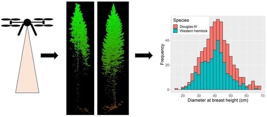
1. Introduction
- Accurately combine field and lidar data to produce training data with high confidence that field trees have been matched to lidar point data;
- Train random forest (RF) classification models to distinguish between two conifer species common to forests of the Pacific Northwest;
- Compare the performance of classification models trained using point cloud metrics computed using height, intensity, and both;
- Compare the performance of a RF model trained using a small subset of height and intensity variables to the performance of a model trained using all variables.
2. Data and Methods
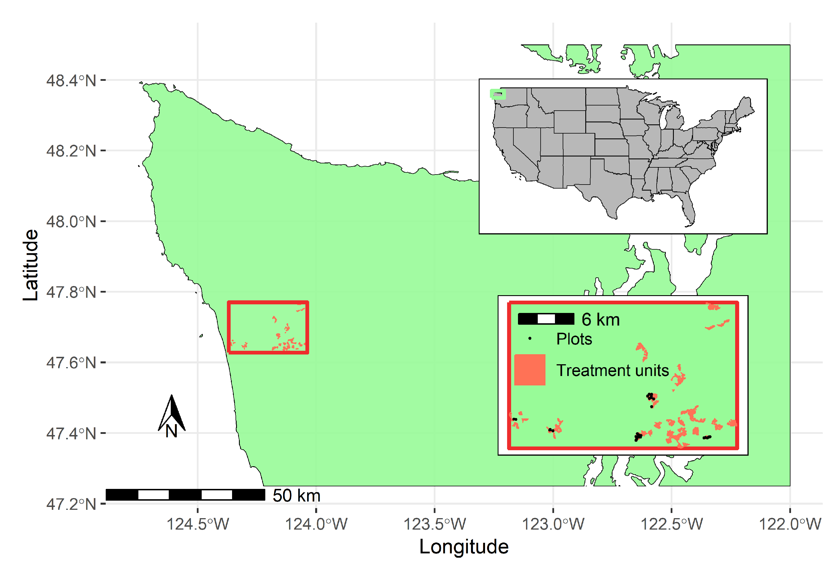
2.1. Study Site
- High net revenue (but not necessarily maximum) within habitat conservation plan sidebars;
- Science-based learning focused on trust management issues;
- Increased public and tribal support for the management of trust lands.
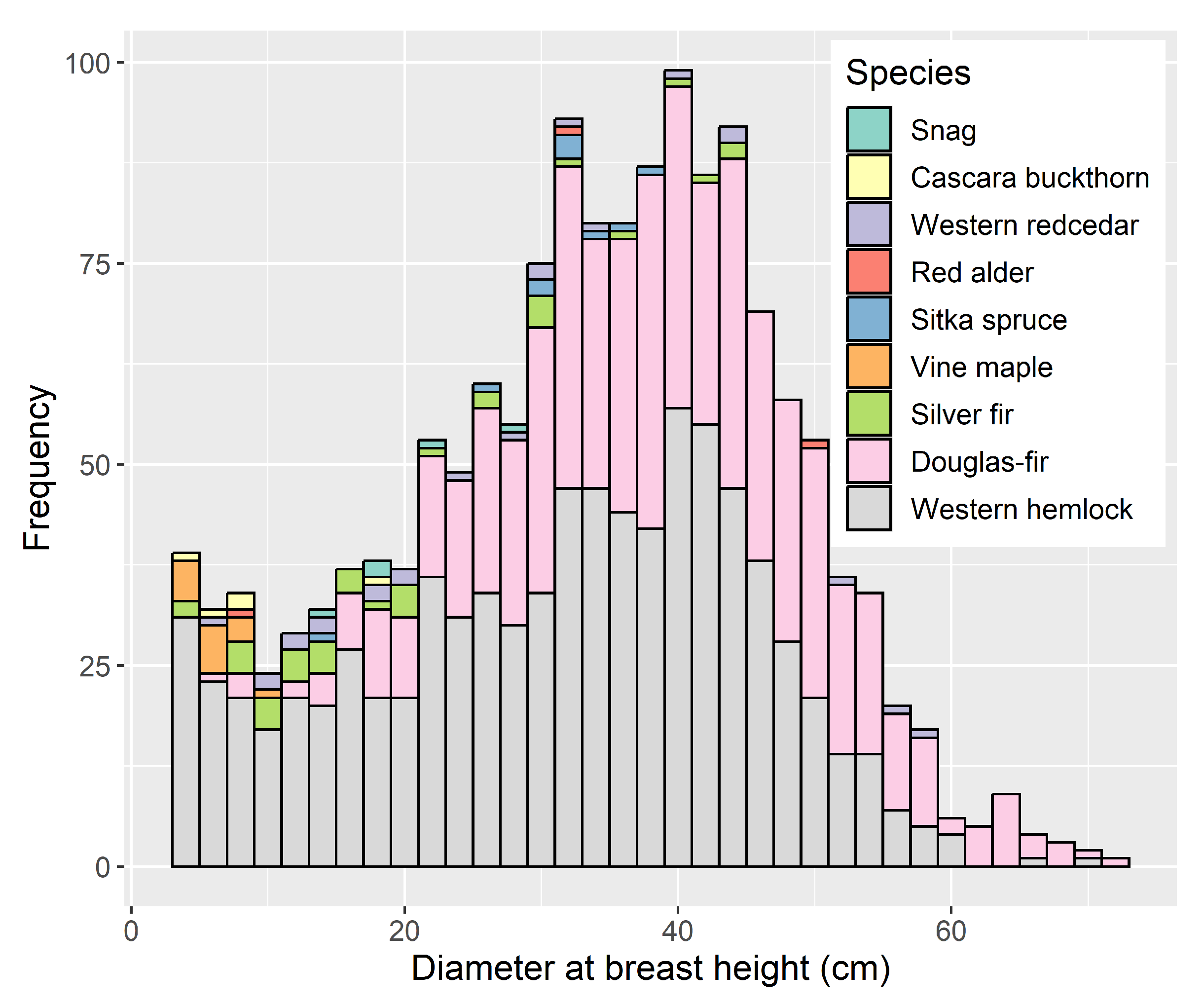
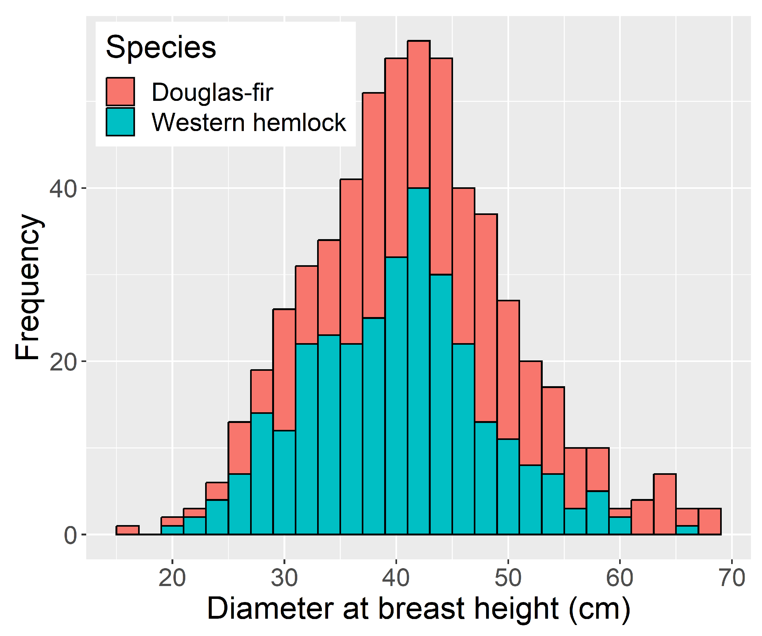
2.2. Field Plots
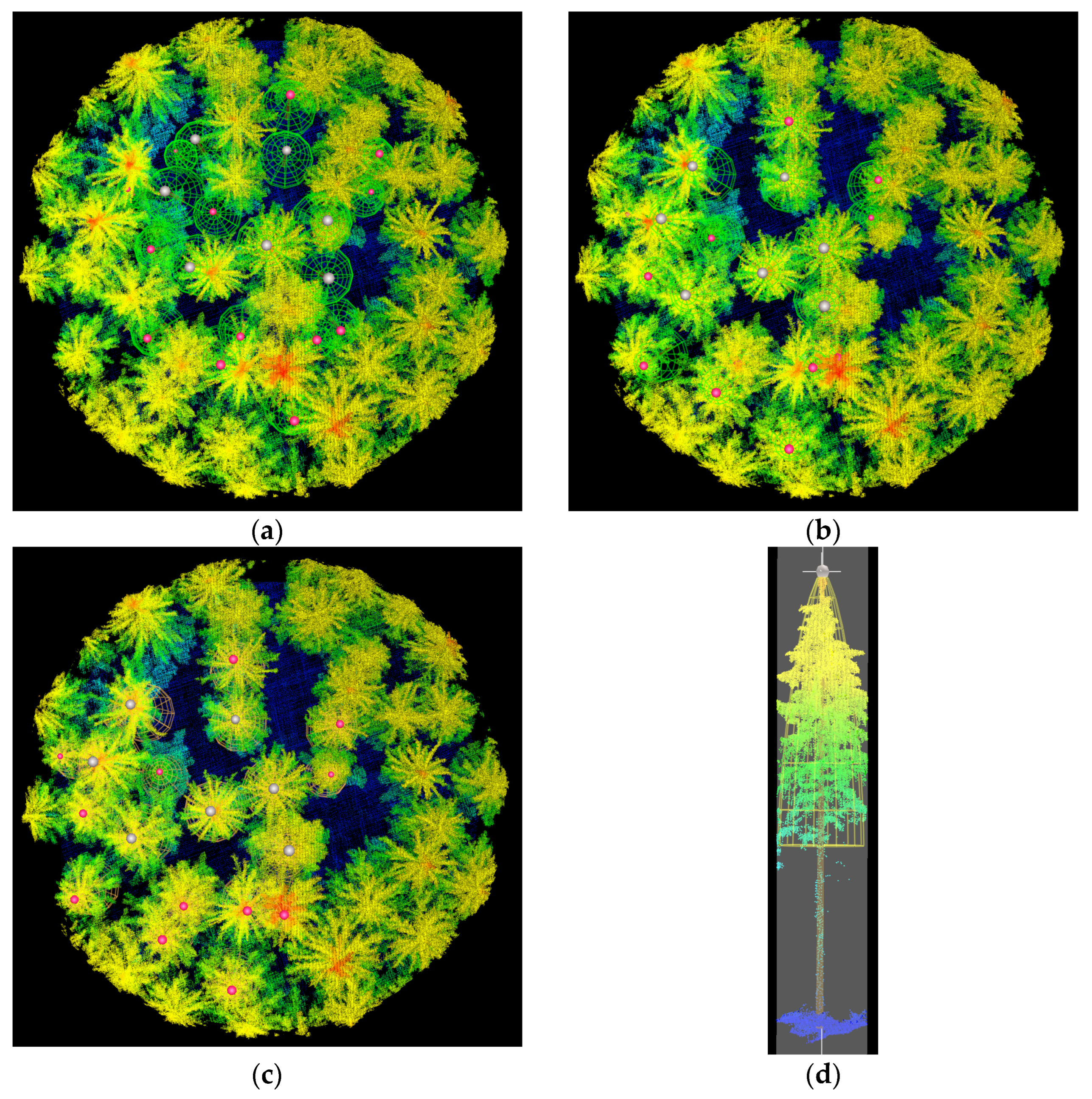
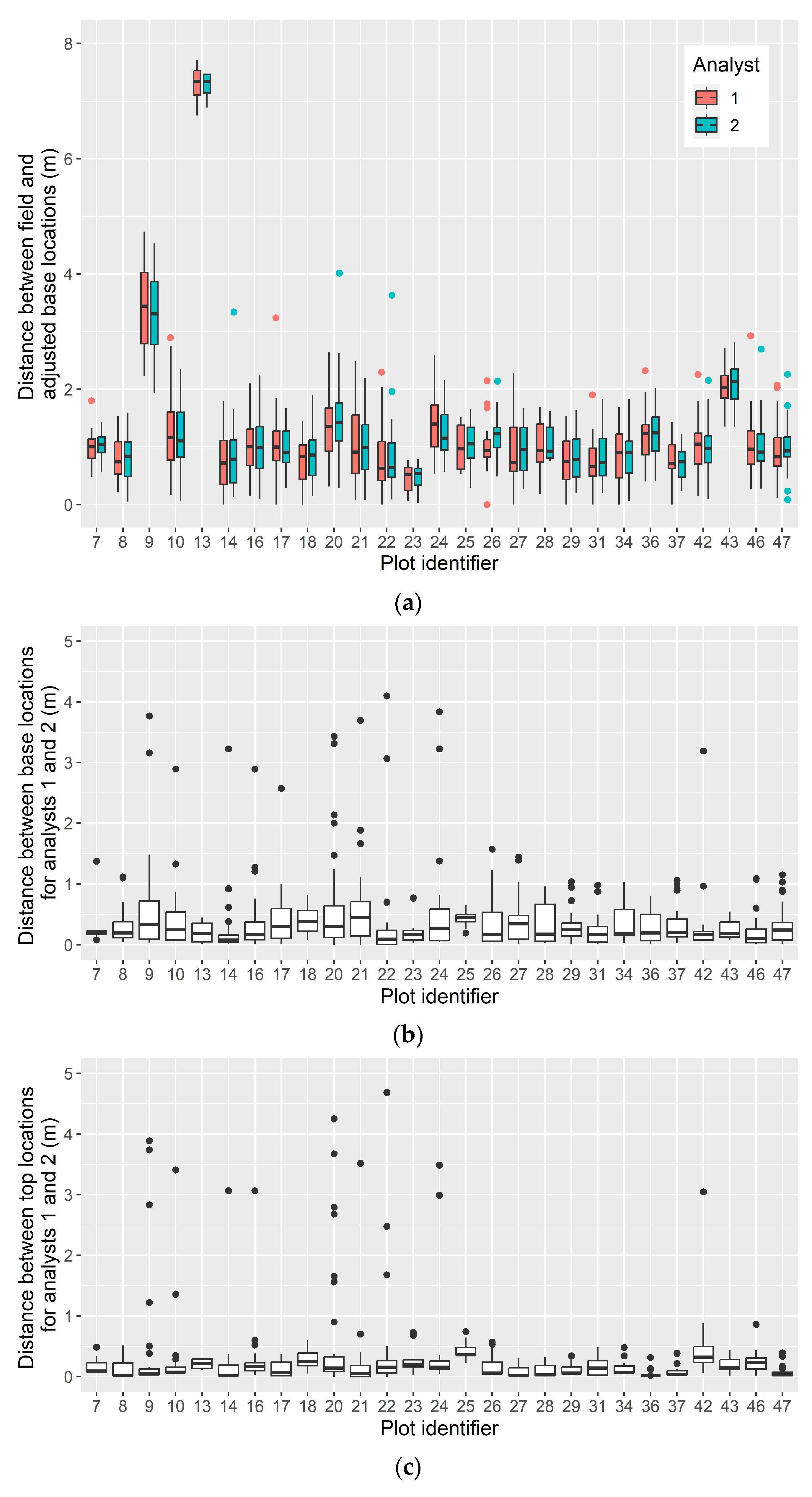
2.2.1. Adjusting Plot and Tree Locations
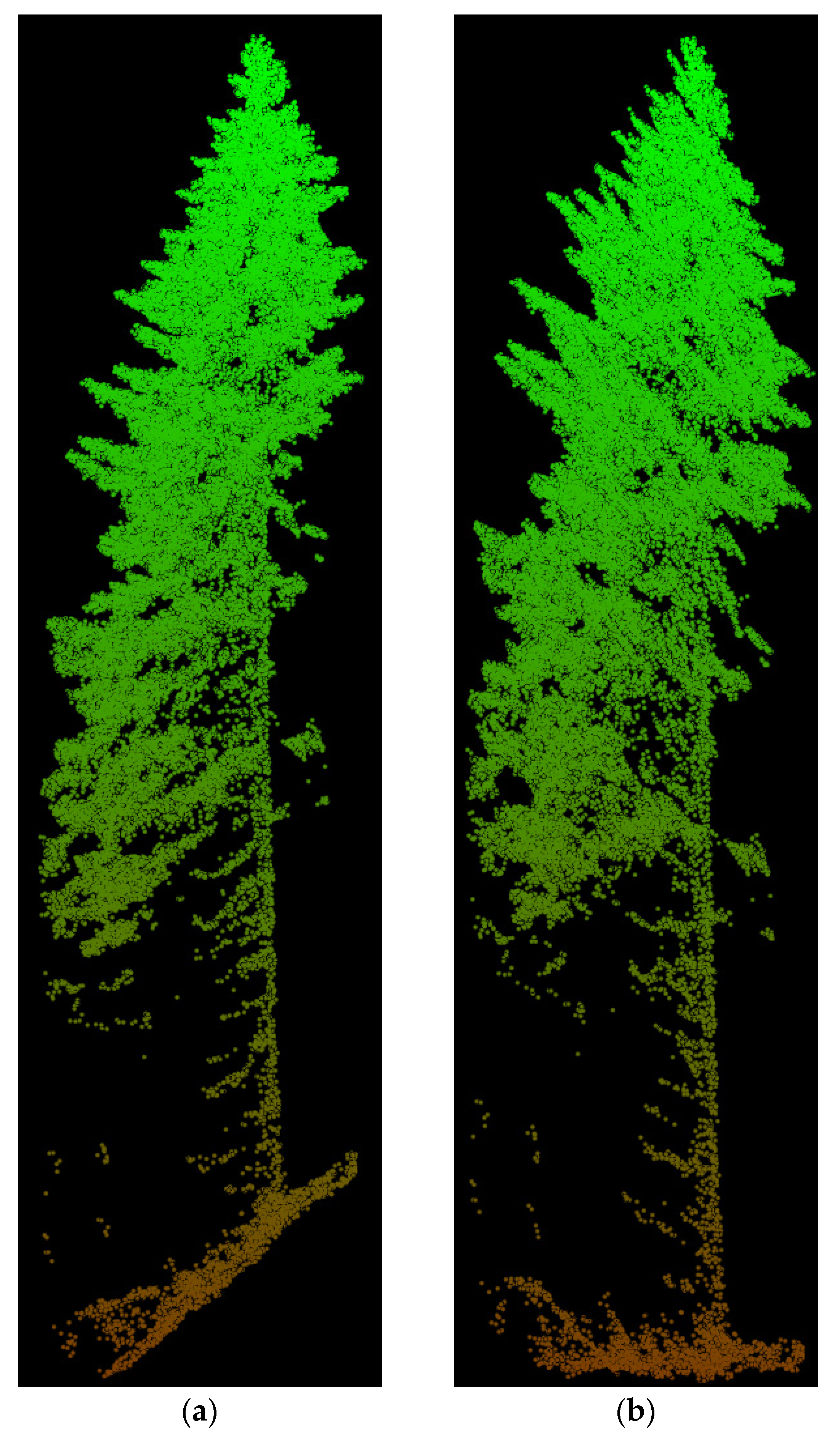
2.3. Lidar Data
Lidar Data Processing
2.4. Model Development
2.5. Model Application
3. Results
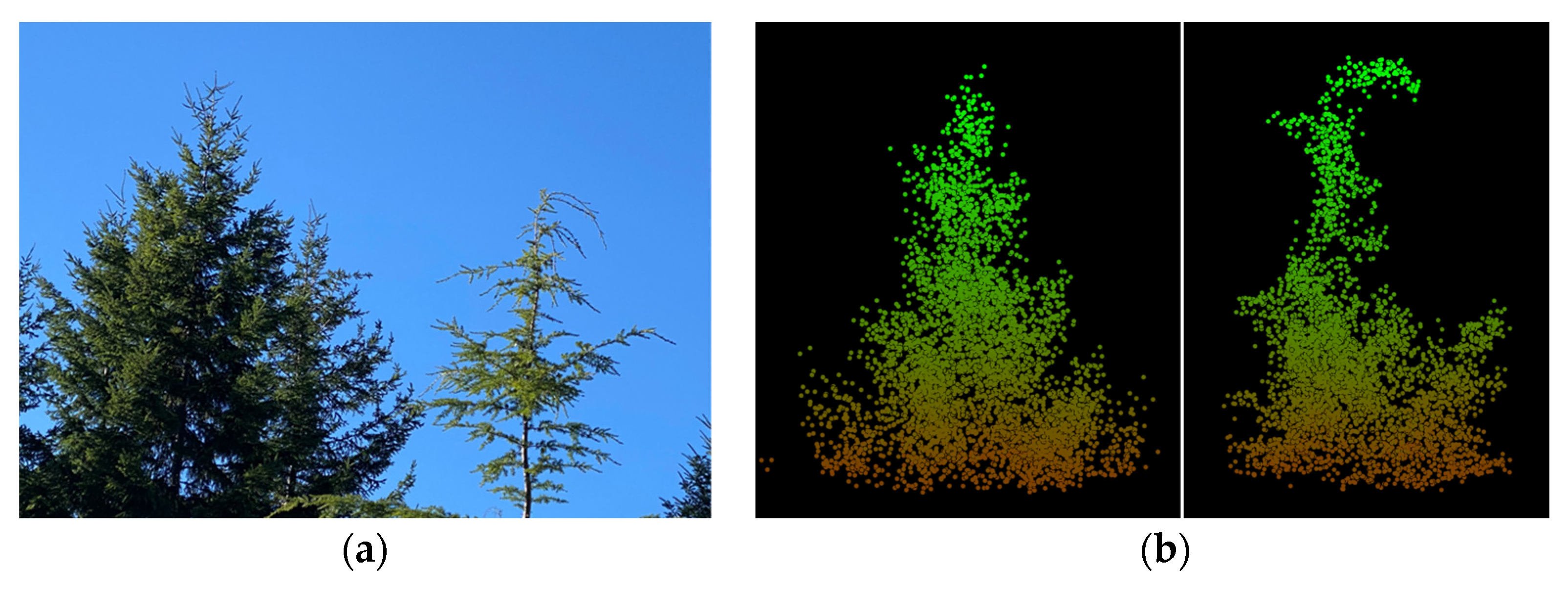
3.1. Confidence in Linking Field Stem Data with Lidar Point Clouds
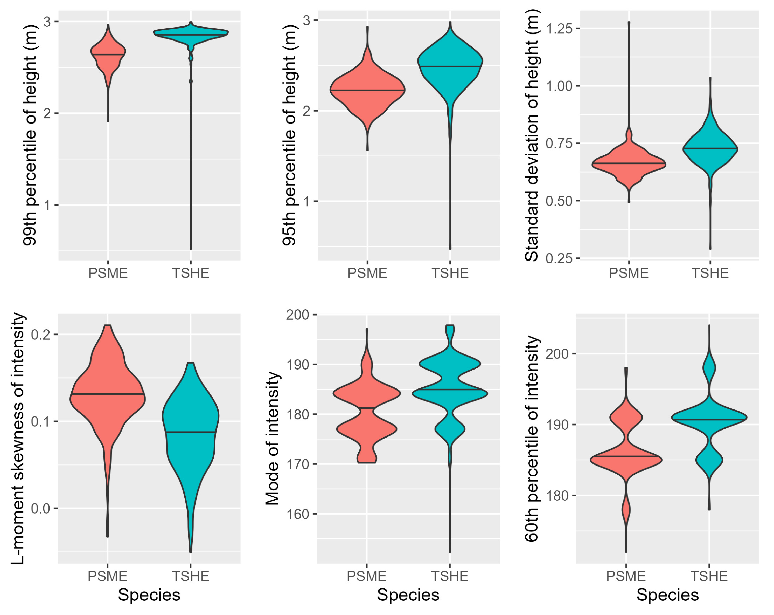
3.2. Model Tuning and Accuracy
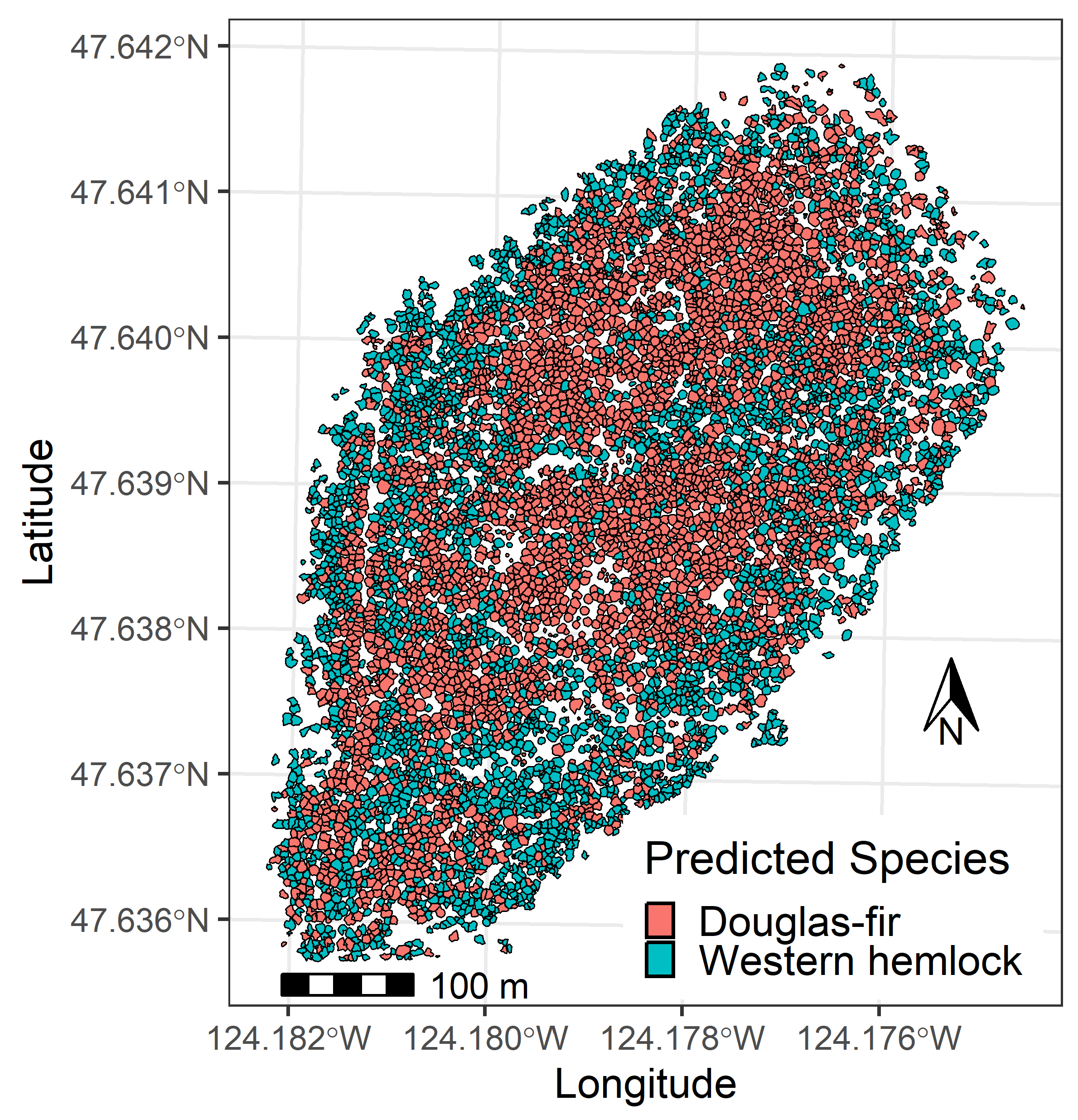
3.3. Model Application
4. Discussion
5. Conclusions
Author Contributions
Funding
Data Availability Statement
Acknowledgments
Conflicts of Interest
References
- Nelson, R.; Krabill, W.; Maclean, G. Determining forest canopy characteristics using airborne laser data. Remote Sens. Environ. 1984, 15, 201–212. [Google Scholar] [CrossRef]
- Nelson, R.; Krabill, W.; Tonelli, J. Estimating forest biomass and volume using airborne laser data. Remote Sens. Environ. 1988, 24, 247–267. [Google Scholar] [CrossRef]
- Nilsson, M. Estimation of tree heights and stand volume using an airborne lidar system. Remote Sens. Environ. 1996, 56, 1–7. [Google Scholar] [CrossRef]
- Næsset, E. Determination of mean tree height of forest stands using airborne laser scanner data. ISPRS J. Photogramm. Remote Sens. 1997, 52, 49–56. [Google Scholar] [CrossRef]
- Næsset, E. Estimating timber volume of forest stands using airborne laser scanner data. Remote Sens. Environ. 1997, 61, 246–253. [Google Scholar] [CrossRef]
- White, J.C.; Wulder, M.A.; Varhola, A.; Vastaranta, M.; Coops, N.C.; Cook, B.D.; Pitt, D.; Woods, M. A Best Practices Guide for Generating Forest Inventory Attributes from Airborne Laser Scanning Data Using an Area-Based Approach; Information Report FI-X-010; Canadian Wood Fibre Centre: Victoria, BC, Canada, 2013. [Google Scholar]
- White, J.C.; Tompalski, P.; Vastaranta, M.; Wulder, M.A.; Saarinen, N.; Stepper, C.; Coops, N.C. A Model Development and Application Guide for Generating an Enhanced Forest Inventory Using Airborne Laser Scanning Data and an Area-Based Approach; Information Report FI-X-018; Canadian Wood Fibre Centre: Victoria, BC, Canada, 2017. [Google Scholar]
- Næsset, E.; Gobakken, T.; Holmgren, J.; Hyyppä, H.; Hyyppä, J.; Maltamo, M.; Nilsson, M.; Olsson, H.; Persson, Å.; Söderman, U. Laser scanning of forest resources: The Nordic experience. Scand. J. For. Res. 2004, 19, 482–499. [Google Scholar] [CrossRef]
- Næsset, E. Practical large-scale forest stand inventory using a small-footprint airborne scanning laser. Scand. J. For. Res. 2004, 19, 164–179. [Google Scholar] [CrossRef]
- Michałowska, M.; Rapinski, J. A review of tree species classification based on airborne LiDAR data and applied classifiers. Remote Sens. 2021, 13, 353. [Google Scholar] [CrossRef]
- Brandtberg, T.; Warner, T.; Landenberger, R.E.; McGraw, J.B. Detection and analysis of individual leaf-off tree crowns in small footprint, high sampling density LIDAR data from the eastern deciduous forest in North America. Remote Sens. Environ. 2003, 85, 290–303. [Google Scholar] [CrossRef]
- Brandtberg, T. Classifying individual tree species under leaf-off and leaf-on conditions using airborne lidar. ISPRS J. Photogramm. Remote Sens. 2007, 61, 325–340. [Google Scholar] [CrossRef]
- Ørka, H.O.; Næsset, E.; Bollandsås, O.M. Classifying Species of Individual Trees by Intensity and Structure Features Derived from Airborne Laser Scanner Data. Remote Sens. Environ. 2009, 113, 1163–1174. [Google Scholar] [CrossRef]
- Liang, X.; Hyyppä, J.; Matikainen, L. Deciduous-coniferous tree classification using difference between first and last pulse laser signatures. IAPRS 2007, 36, 253–257. [Google Scholar]
- Li, J.; Hu, B.; Noland, T.L. Classification of tree species based on structural features derived from high density LiDAR data. Agric. For. Meteorol. 2013, 171, 104–114. [Google Scholar] [CrossRef]
- Sun, P.; Yuan, X.; Li, D. Classification of individual tree species using UAV LiDAR based on transformer. Forests 2023, 14, 484. [Google Scholar] [CrossRef]
- Qian, C.; Yao, C.; Ma, H.; Xu, J.; Wang, J. Tree species classification using airborne LiDAR data based on individual tree segmentation and shape fitting. Remote Sens. 2023, 15, 406. [Google Scholar] [CrossRef]
- Horn, H.S. The Adaptive Geometry of Trees; Princeton University Press: Princeton, NJ, USA, 1971. [Google Scholar]
- Valladares, F.; Niinemets, Ü. The architecture of plant crowns: From design rules to light capture and performance. In Functional Plant Ecolology, 2nd ed.; Pugnaire, F.F., Valladares, F., Eds.; CRC Press: Boca Raton, FL, USA, 2007; pp. 101–150. [Google Scholar] [CrossRef]
- Hackenberg, J.; Spiecker, H.; Calders, K.; Disney, M.; Raumonen, P. SimpleTree-An efficient open source tool to build tree models from TLS clouds. Forests 2015, 6, 4245–4294. [Google Scholar] [CrossRef]
- Harikumar, A.; Bovolo, F.; Bruzzone, L. An internal crown geometric model for conifer species classification with high-density LiDAR data. IEEE Trans. Geosci. Remote Sens. 2017, 55, 2924–2940. [Google Scholar] [CrossRef]
- Stoker, J.; Miller, B. The accuracy and consistency of 3D elevation program data: A systematic analysis. Remote Sens. 2022, 14, 940. [Google Scholar] [CrossRef]
- Cárdenas, J.L.; López, A.; Ogayar, C.J.; Feito, F.R.; Jurado, J.M. Reconstruction of tree branching structures from UAV-LiDAR data. Front. Environ. Sci. 2022, 10, 960083. [Google Scholar] [CrossRef]
- Washington Department of Natural Resources. Mill Log Prices—Domestically Processed. 2023. Available online: https://www.dnr.wa.gov/publications/psl_ts_jan23_logprices.pdf (accessed on 15 December 2023).
- Washington Department of Natural Resources. Olympic Experimental State Forest Website. 2023. Available online: https://www.dnr.wa.gov/oesf (accessed on 15 December 2023).
- Bormann, B.T.; Minkova, T. The T3 Watershed Experiment Upland Silviculture Study Plan; University of Washington and Washington Department of Natural Resources: Olympia, WA, USA, 2022. Available online: https://www.dnr.wa.gov/sites/default/files/publications/lm_oesf_t3_upland_pln.pdf (accessed on 1 February 2024).
- McGaughey, R.J.; Ahmed, K.; Andersen, H.-E.; Reutebuch, S.E. Effect of occupation time on the horizontal accuracy of a mapping-grade GNSS receiver under dense forest canopy. Photogramm. Eng. Remote Sens. 2017, 83, 861–868. [Google Scholar] [CrossRef]
- Andersen, H.-E.; Strunk, J.; McGaughey, R.J. Using High-Performance Global Navigation Satellite System Technology to Improve Forest Inventory and Analysis Plot Coordinates in the Pacific Region; Gen. Tech. Rep. PNW-GTR-1000; U.S. Department of Agriculture, Forest Service, Pacific Northwest Research Station: Portland, OR, USA, 2022; 38p.
- FVS Staff. Pacific Northwest Coast (PN) Variant Overview-Forest Vegetation Simulator. Internal Report; (Revised 22 December 2022); U.S. Department of Agriculture, Forest Service, Forest Management Service Center: Fort Collins, CO, USA, 2008; 75p. Available online: https://www.fs.usda.gov/fmsc/ftp/fvs/docs/overviews/FVSpn_Overview.pdf (accessed on 15 December 2023).
- McGaughey, R.J. FUSION/LDV: Software for LIDAR Data Analysis and Visualization. 2023. Available online: http://forsys.sefs.uw.edu/software/fusion/FUSION_manual.pdf (accessed on 1 February 2024).
- Hothorn, T.; Hornik, K.; van de Wiel, M.; Zeileis, A. A lego system for conditional inference. Am. Stat. 2006, 60, 257–263. [Google Scholar] [CrossRef]
- R Core Team. R: A Language and Environment for Statistical Computing; R Foundation for Statistical Computing: Vienna, Austria, 2023; Available online: https://www.R-project.org/ (accessed on 1 February 2024).
- Roussel, J.R.; Auty, D.; Coops, N.C.; Tompalski, P.; Goodbody, T.R.H.; Sánchez Meador, A.; Bourdon, J.F.; De Boissieu, F.; Achim, A. lidR: An R package for analysis of airborne laser scanning (ALS) data. Remote Sens. Environ. 2020, 251, 112061. [Google Scholar] [CrossRef]
- Roussel, J.-R.; Auty, D. Airborne LiDAR data Manipulation and Visualization for Forestry Applications. R package Version 4.0.4. 2023. Available online: https://cran.r-project.org/package=lidR (accessed on 1 February 2024).
- McGaughey, R.J. Fusionwrapr Package. Available online: https://github.com/bmcgaughey1/fusionwrapr (accessed on 15 December 2023).
- Hosking, J.R.M. L-moments: Analysis and estimation of distributions using linear combinations of order statistics. J. R. Stat. Soc. Ser. B Methodol. 1990, 52, 105–124. [Google Scholar] [CrossRef]
- Wang, O.J. Direct sample estimators of L moments. Water Resour. Res. 1996, 32, 3617–3619. [Google Scholar] [CrossRef]
- Hu, T.; Ma, Q.; Su, Y.; Battles, J.J.; Collins, B.M.; Stephens, S.L.; Kelly, M.; Guo, Q. A simple and integrated approach for fire severity assessment using bi-temporal airborne LiDAR data. Int. J. Appl. Earth Obs. Geoinf. 2019, 78, 25–38. [Google Scholar] [CrossRef]
- Probst, P.; Wright, M.N.; Boulesteix, A.-L. Hyperparameters and tuning strategies for random forest. WIRES Data Min. Knowl. 2019, 9, e1301. [Google Scholar] [CrossRef]
- Probst, P.; Boulesteix, A.-L. To tune or not to tune the number of trees in random forest. J. Mach. Learn. Res. 2018, 18, 1–18. [Google Scholar]
- Wright, M.N.; Ziegler, A. ranger: A fast implementation of random forests for high dimensional data in C++ and R. J. Stat. Softw. 2017, 77, 1–17. [Google Scholar] [CrossRef]
- Hinkle, D.E.; Wiersma, W.; Jurs, S.G. Applied Statistics for the Behavioral Sciences; Houghton Mifflin: Boston, MA, USA, 2003; Volume 663, ISBN 10:0618124055/13:9780618124053. [Google Scholar]
- Lin, Y.; Hyyppä, J. A comprehensive but efficient framework of proposing and validating feature parameters from airborne LiDAR data for tree species classification. Int. J. Appl. Earth Obs. Geoinf. 2016, 46, 45–55. [Google Scholar] [CrossRef]
- Fassnacht, F.; Latifi, H.; Stereńczak, K.; Modzelewska, A.; Lefsky, M.; Waser, L.; Straub, C.; Ghosh, A. Review of studies on tree species classification from remotely sensed data. Remote Sens. Environ. 2016, 186, 64–87. [Google Scholar] [CrossRef]
- Korpela, I.; Koskinen, M.; Vasander, H.; Holopainen, M.; Minkkinen, K. Airborne small-footprint discrete-return LiDAR data in the assessment of boreal mire surface patterns, vegetation and habitats. For. Ecol. Manag. 2009, 258, 1549–1566. [Google Scholar] [CrossRef]
- Mielcarek, M.; Stereńczak, K.; Khosravipour, A. Testing and evaluating different LiDAR-derived canopy height model generation methods for tree height estimation. Int. J. Appl. Earth Obs. Geoinf. 2018, 71, 132–143. [Google Scholar] [CrossRef]
- Zhao, K.; Popescu, S. Hierarchical watershed segmentation of canopy height model for multi-scale forest inventory. Proc. ISPRS Work. Group 2007, 442, 436. [Google Scholar]
- Van Pelt, R.; Sillett, S.C. Crown development of coastal pseudotsuga menziesii, including a conceptual model for tall conifers. Ecol. Monogr. 2008, 78, 283–311. [Google Scholar] [CrossRef]
- Hell, M.; Brandmeier, M.; Briechle, S.; Krzystek, P. Classification of Tree Species and Standing Dead Trees with Lidar Point Clouds Using Two Deep Neural Networks: PointCNN and 3DmFV-Net. PFG 2022, 90, 103–121. [Google Scholar] [CrossRef]
- Hao, Z.; Wenshu, L.; Haoran, L.; Nan, M.; Kangkang, L.; Rongzhen, C.; Tiantian, W.; Zhengzhao, R. Identification of tree species based on the fusion of UAV hyperspectral image and LiDAR data in a coniferous and broad-leaved mixed forest in Northeast China. Front. Plant Sci. 2022, 13, 964769. [Google Scholar] [CrossRef]


| Metric Name | Computed for Height | Computed for Intensity | Description |
|---|---|---|---|
| Minimum, maximum, mean, mode, standard deviation, variance, coefficient of variation, interquartile distance, skewness, kurtosis, average absolute difference | X | X | Standard descriptive statistics. Minimum and maximum height were dropped from the set of variables because we expect these to have nearly the same values for all trees: minimum = 0 and maximum = 3. |
| MAD.median | X | Average distance between each data point and the median. | |
| MAD.mode | X | Average distance between each data point and the mean. | |
| L-moments | X | X | L moments are computed using linear combinations of ordered data values (elevation and intensity) [36]. The first four L moments (L1, L2, L3, L4) are estimated using the direct sample estimators proposed by Wang [37]. L1 is exactly equal to the mean. |
| L-moment ratios | X | X | Ratios of L moments provide statistics that are comparable to the coefficient of variation (L2/L1), skewness (L3/L2) and kurtosis (L4/L2). |
| Percentiles | X | X | Height or intensity value below which a given percentage, k, of values in the frequency distribution falls. k = (1, 5, 10, 20, 25, 30, 40, 50, 60, 70, 75, 80, 90, 95, 99). |
| Canopy relief ratio | X | ||
| SQRT.mean.SQ | X | ||
| CURT.mean.CUBE | X | ||
| Profile area | X | Modified version of the area under the height percentile curve described by Hu et al. [38]. Modifications to the calculation method are described in McGaughey’s work [30]. | |
| Relative percentile heights | X | Percentile height, k, divided by the 99th percentile height with k = (1, 5, 10, 20, 25, 30, 40, 50, 60, 70, 75, 80, 90, 95). |
| Predictors | mtry | min.node.size | sample.fraction | Accuracy (%) | Kappa |
|---|---|---|---|---|---|
| Height and intensity | 12 | 2 | 0.46858 | 91.8 | 0.83 |
| Height only | 22 | 18 | 0.20776 | 88.7 | 0.77 |
| Intensity only | 28 | 21 | 0.51976 | 78.6 | 0.57 |
| Subset | 1 | 3 | 0.20687 | 91.5 | 0.83 |
Disclaimer/Publisher’s Note: The statements, opinions and data contained in all publications are solely those of the individual author(s) and contributor(s) and not of MDPI and/or the editor(s). MDPI and/or the editor(s) disclaim responsibility for any injury to people or property resulting from any ideas, methods, instructions or products referred to in the content. |
© 2024 by the authors. Licensee MDPI, Basel, Switzerland. This article is an open access article distributed under the terms and conditions of the Creative Commons Attribution (CC BY) license (https://creativecommons.org/licenses/by/4.0/).
Share and Cite
McGaughey, R.J.; Kruper, A.; Bobsin, C.R.; Bormann, B.T. Tree Species Classification Based on Upper Crown Morphology Captured by Uncrewed Aircraft System Lidar Data. Remote Sens. 2024, 16, 603. https://doi.org/10.3390/rs16040603
McGaughey RJ, Kruper A, Bobsin CR, Bormann BT. Tree Species Classification Based on Upper Crown Morphology Captured by Uncrewed Aircraft System Lidar Data. Remote Sensing. 2024; 16(4):603. https://doi.org/10.3390/rs16040603
Chicago/Turabian StyleMcGaughey, Robert J., Ally Kruper, Courtney R. Bobsin, and Bernard T. Bormann. 2024. "Tree Species Classification Based on Upper Crown Morphology Captured by Uncrewed Aircraft System Lidar Data" Remote Sensing 16, no. 4: 603. https://doi.org/10.3390/rs16040603
APA StyleMcGaughey, R. J., Kruper, A., Bobsin, C. R., & Bormann, B. T. (2024). Tree Species Classification Based on Upper Crown Morphology Captured by Uncrewed Aircraft System Lidar Data. Remote Sensing, 16(4), 603. https://doi.org/10.3390/rs16040603