Abstract
Soil organic matter (SOM) is an essential component of soil and is crucial for increasing agricultural production and soil fertility. The combination of hyperspectral remote sensing and deep learning can be used to predict the SOM content efficiently, rapidly, and cost-effectively on various scales. However, determining the optimal groups, inputs, and models for reducing the spatial heterogeneity of soil nutrients in large regions and to improve the accuracy of SOM prediction remains a challenge. Hyperspectral reflectance data from 1477 surface soil samples in Northeast China were utilized to evaluate three grouping methods (no groups (NG), traditional grouping (TG), and spectral grouping (SG)) and four inputs (raw reflectance (RR), continuum removal (CR), fractional-order differentiation (FOD), and spectral characteristic parameters (SCPs)). The SOM prediction accuracies of random forest (RF), convolutional neural network (CNN), and long short-term memory (LSTM) models were assessed. The results were as follows: (1) The highest accuracy was achieved using SG, SCPs, and the LSTM model, with a coefficient of determination (R2) of 0.82 and a root mean squared error (RMSE) of 0.69%. (2) The LSTM model exhibited the highest accuracy in SOM prediction (R2 = 0.82, RMSE = 0.89%), followed by the CNN model (R2 = 0.72, RMSE = 0.85%) and the RF model (R2 = 0.69, RMSE = 0.91%). (3) The SG provided higher SOM prediction accuracy than TG and NG. (4) The SCP-based prediction results were significantly better than those of the other inputs. The R2 of the SCP-based model was 0.27 higher and the RMSE was 0.40% lower than that of the RR-based model with NG. In addition, the LSTM model had higher prediction errors at low (0–2%) and high (8–10%) SOM contents, whereas the error was minimal at intermediate SOM contents (2–8%). The study results provide guidance for selecting grouping methods and approaches to improve the prediction accuracy of the SOM content and reduce the spatial heterogeneity of the SOM content in large regions.
1. Introduction
Soil organic matter (SOM) is a critical indicator of soil quality and fertility and resource evaluation. Hyperspectral remote sensing can be used to monitor soil properties rapidly and is less time-consuming and costly than traditional methods [1]. It can be used to predict soil properties using soil spectral information and is a fast, accurate, quantitative, and cost-effective method for predicting SOM [2]. Numerous studies have shown that hyperspectral techniques are applicable in the 350–2500 nm wavelength [3,4]. Absorption features in soils are attributed to the fundamental vibrations of functional groups, such as C=O, O-H, N-H, and C-H, which exhibit their overtones and combinatorial bands in a specific spectral wavelength range [5,6]. Therefore, we can detect the presence of different functional groups in soils and accurately estimate soil properties by analyzing the spectral reflectance data of soils.
Spectral reflectance data are frequently confounded by factors that introduce substantial noise and reduce the accuracy of prediction models [7]. The noise in spectral reflectance data is often attributed to interference from multiple factors [7]. Preprocessing is required to improve data quality and model performance. Typical preprocessing methods for spectral data include Savitzky–Golay convolutional smoothing (S-G), continuum removal (CR), resampling, mathematical transforms, and other methods [8,9]. These methods can effectively mitigate noise and improve the accuracy and credibility of the data, providing suitable data for establishing prediction models with high performance. CR highlights the absorption and reflection features within the spectrum [10], and the CR curve can be used to extract the spectral characteristic parameters (SCPs) used for soil classification and prediction. SCP extraction is generally used to distinguish the differences in the spectral features of samples in the same soil class, different soil genera, or the same soil genus and different soil species [11]. Therefore, the metrics extracted by SCPs can reflect the shape and absorption features of the spectra. Bayer et al. [12] successfully used SCPs for soil property prediction. Laukamp et al. [13] extracted characteristic parameters related to soil mineral abundance and composition from shortwave, mid-wave, and thermal infrared reflectance spectra, bridging the gap between mineral diagnostic absorption features and the accurate interpretation of reflectance spectra. They extracted geologically relevant information from reflectance spectra. A commonly used mathematical transformation is the first-order differential [14]. Fractional-order differentiation (FOD) is suitable for discrete and continuous data and better amplifies the subtle differences between spectral curves with nonlinear characteristics than integer-order differentiation [15]. However, the predictive power of different input quantities has yet to be verified for large regions.
Spatial heterogeneity exists in the SOM distribution in different regions due to differences in soil types and environmental conditions. The relationship between soil spectral reflectance and soil properties is intricate and nonlinear due to differences in soil parent material, topography, climate, and geology. Consequently, the rational grouping of soil samples is essential for the prediction of SOM content. The effects of different soil types and spectral characteristics on the SOM content were clarified by using different grouping methods [16,17] and selecting appropriate prediction models and feature extraction methods, improving the model’s prediction accuracy and generalization ability. Standard grouping methods are divided into three categories. The first is based on soil physicochemical properties. Jaconi et al. [18] used memory-based learning (MBL) to assess soil properties (depth, pH, and soil texture) and grouped the datasets to reduce the error in predicting soil organic carbon. The second category is land use/land cover-based grouping (e.g., forest, grassland, and farmland) [19]. For example, Xu et al. [20] used different soil types, including mineral and organic soils, to analyze the effects of different factors on the SOM content. The third category is a grouping of the soil samples into several clusters with similar spectral features [21,22]. Ramirez-Lopez et al. [23] proposed a spectral-based learner (SBL) that uses an optimized principal component distance (oPC-M) to measure the spectral similarity between soil samples. Based on the spectral similarity, a local sample set is selected as the target domain for the prediction. Soil properties were predicted within the target domain using Gaussian process regression. The methodology and accuracy of SOM prediction approaches have room for improvement. Most studies used single-factor classification. Comprehensive models can be used to capture the interactions of different factors and improve prediction accuracy. Machine learning and deep learning can process multi-source data and mine them for potential patterns. Machine learning algorithms reveal nonlinear relationships between independent and dependent variables, while deep learning, through multi-layer neural networks, can extract deeper nonlinear relationships between input variables and soil properties. For highly nonlinear research problems, deep learning models have a greater advantage compared to machine learning. Feature selection aids in extracting crucial features and reducing dimensionality. The accuracy and reliability of SOM prediction can be enhanced by selecting multiple factors, using advanced techniques, and optimizing the prediction model.
Due to the rapid development of deep learning technology, a transformation from machine learning to deep learning has occurred. Deep learning models demonstrate strong potential for SOM content prediction, as they are capable of unveiling the nonlinear relationships between the reflectance spectra and soil properties. The results are generally better than those obtained from traditional machine learning models [24]. For example, convolutional neural networks (CNNs) and long short-term memory networks (LSTMs) can learn complex spatial and temporal features from hyperspectral data to capture the relationship between soil spectra and SOM content [25]. Unlike traditional machine learning algorithms, deep learning models can automatically learn features, eliminating the need for the laborious process of manually designing features using traditional methods. Deep learning network models have been widely used in soil spectroscopy to extract features from input data more accurately, significantly improving prediction performance and efficiency [26,27]. However, the prediction ability of different models coupled with different grouping methods in large regions with substantial spatial heterogeneity of the SOM requires improvement.
This study investigates the optimal combination of models, inputs, and grouping methods for SOM content prediction. We use 1477 surface soil (0–20 cm) samples from the northeast region of China and predict the SOM content prediction using three models (random forest (RF), CNN, and LSTM), three grouping methods (no groups (NG), traditional grouping (TG), and spectral grouping (SG)), and four inputs (raw reflectance (RR), CR, FOD, and SCPs). The objectives of this study are (1) to compare the accuracy of the models for different inputs and the optimal combination of inputs and predictive models and (2) to determine the effect of different grouping methods on the accuracy of SOM content prediction. This study’s results will contribute to optimizing SOM content prediction models, thereby enhancing the accuracy and reliability of soil property prediction. This will serve as a valuable reference for large-scale farmland soil fertility assessments and agricultural production.
2. Materials and Methods
2.1. Overview of the Study Area
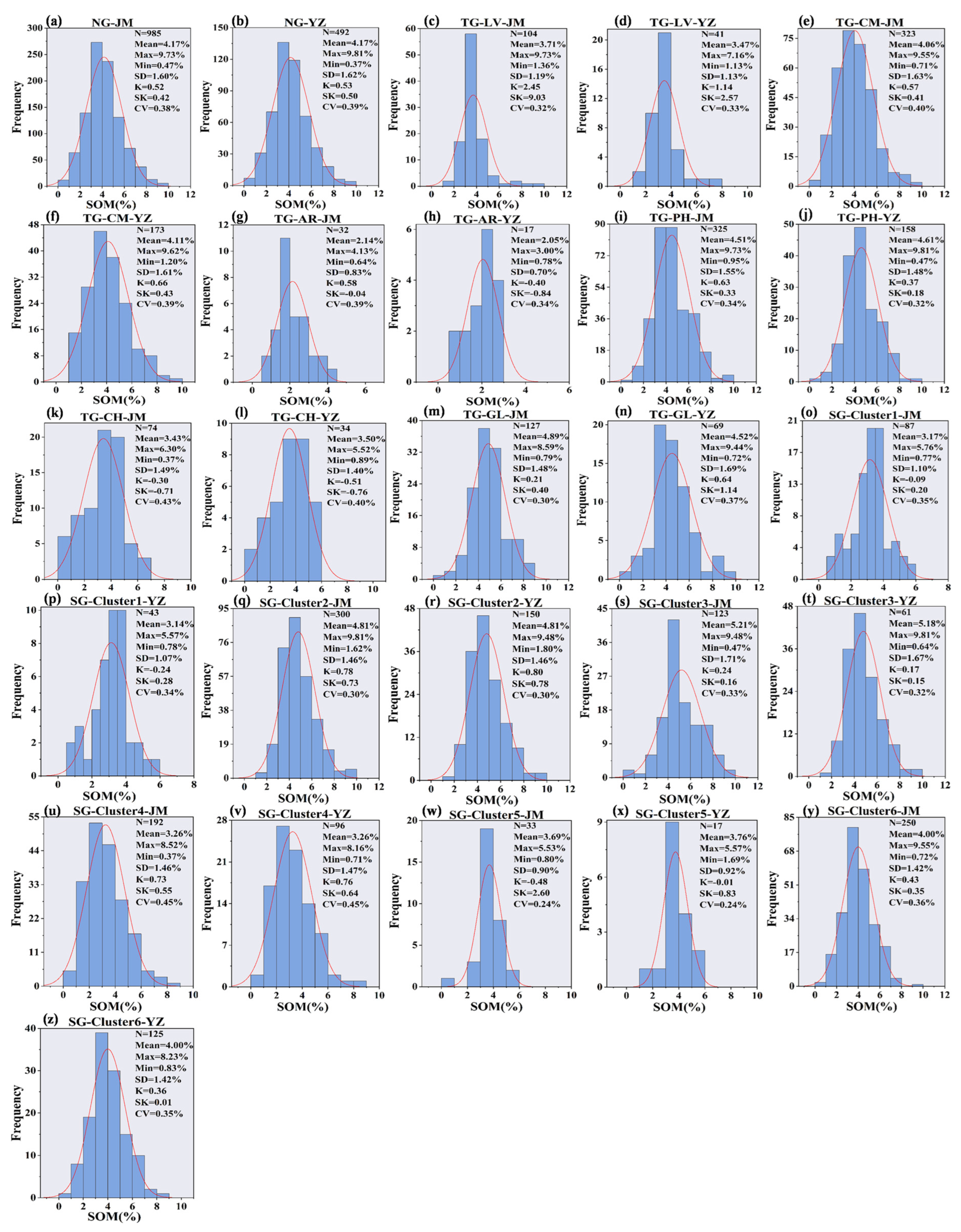
The study area was the northeastern region of China, which includes Heilongjiang, Jilin, Liaoning, and the four eastern leagues of Inner Mongolia (115.52°E–135.09°E and 38.72°N–53.56°N). The area is approximately 1,030,000 km2 and has a temperate continental monsoon climate. Annual precipitation ranges from 300 to 950 mm, with an average of 506 mm. It decreases from southeast to northwest. The landforms include plains, plateaus, hills, and mountains, and the soil types are dominated by Phaeozems, Chernozems, Cambisols, dark brown loams, Arenosols, Luvisols, Gleysols, and other soil types.
Phaeozems have a thick soil layer with a good soil structure, loose soil texture, good drainage, high water-holding capacity, and high organic matter content. Chernozems have a deep humus layer, and the lower and middle parts are calcium carbonate deposits with high potential fertility. Gleysols are composed of a peat layer (T-layer) and a submerged layer (G-layer). The former is rich in organic matter, and the latter has an organic matter content of 11.0%. The parent material of Luvisols is mainly composed of Quaternary river and lake sediments, with a barren layer of a white slurry, which has a sticky and heavy texture and low water permeability. Arenosols have a lower organic matter content than Phaeozems and Chernozems, a loose soil structure, and a fine sandy texture. They have low water and fertilizer retention capacity and are susceptible to wind and water erosion. Cambisols are typically located in low-lying terrains, often interspersed among other soil types. They have high porosity, high organic matter content, and good aeration and are susceptible to wind erosion, resulting in low topsoil quality.
2.2. Soil Sample Collection and Processing
We collected 1477 topsoil samples from the 0–20 cm layer in the northeast (Figure 1), including Luvisol, Cambisol, Arenosol, Phaeozem, Chernozem, and Gleysol samples (Table 1). The soil samples were air-dried and milled to obtain a particle size smaller than 2 mm. Each soil sample was divided into two parts, one for spectroscopic measurements and the other for the analysis of the SOM content (%). We obtained reflectance spectra of the soil samples for subsequent analyses. The organic carbon content was determined by the high-temperature exothermic potassium dichromate oxidative capacity method [28]. The resulting value was multiplied by 1.724 to convert it to SOM content [29].

Figure 1.
Distribution of soil sampling sites in the study area.

Table 1.
Statistics on the number of each soil sample.
2.3. Soil Spectrometry
A FieldSpec@3 portable spectrometer (Analytical Spectral Devices (ASD), Boulder, CO, USA) was used in the laboratory to obtain the spectra of the soil samples. The soil samples were scraped with a straightedge, and the collected material was placed in dishes with a diameter of 12 cm and a depth of 1.8 cm. A 50 W halogen lamp 100 cm from the soil sample surface was used as the light source, with a zenith angle of 30°. The light was parallel to the soil sample surface to minimize the shadow effect caused by soil roughness. A sensor probe with an 8° field of view was placed 15 cm from the surface and perpendicular to the soil sample. The impact of the dark current was eliminated before testing, and calibration was performed with a whiteboard. Ten spectral curves were obtained for each soil sample, and the arithmetic mean was calculated and utilized for subsequent analysis.
2.4. Spectral Data Preprocessing
Most of the noise is concentrated in the ranges of 350–430 nm and 2400–2500 nm; therefore, we selected 430–2400 nm as the wavelength range [30]. The following processing methods were adopted to eliminate spectral noise and redundant information and enhance the quality of the spectral data.
- (1)
- Savitzky–Golay convolutional smoothing (S-G)
Smoothing is a standard preprocessing method used in spectral analysis [31]. The spectral data were smoothed using S-G and a 9 × 9 window to reduce noise interference [32,33]. The spectral library function in ENVI version 5.3 was used to resample the spectral reflectance data to 10 nm [34]. The result was the initial reflectance (RR) data.
- (2)
- Continuum removal (CR)
CR is used to normalize the reflectance spectra. It removes baseline drift and background noise from the spectrum and improves spectral accuracy and stability [35]. Each peak has a value of 1 after CR, and the non-peak values are less than 1, resulting in reflectance values in the range of 0–1. CR enables the comparison of reflectance values across various spectral bands. This allowed us to highlight the absorption and reflection characteristics of different soils, enhancing the variability of different soils and facilitating the extraction of features and classification analyses.
- (3)
- Spectral characteristic parameters (SCPs)
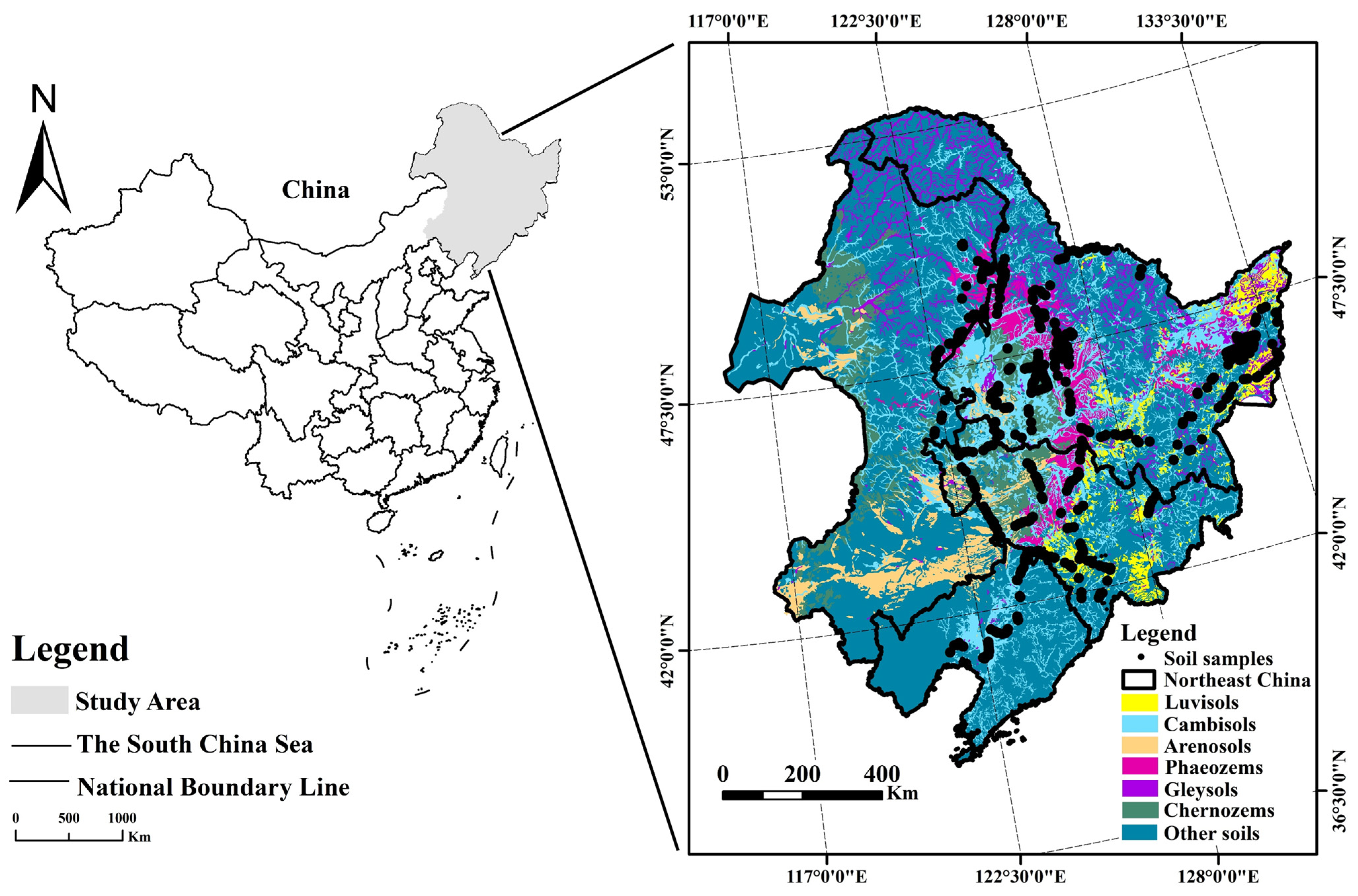
The extraction of the SCPs was based on the shape of the CR spectral curve to obtain accurate parameters. Five key absorption valleys (V1–V5) were extracted, and the SOM content was predicted by assessing the characteristics of the first two absorption valleys (V1 and V2). The SOM content affects V1 and V2, whereas the soil moisture content influences V3, V4, and V5. Sixteen SCPs were selected based on the spectral characteristics of the soil samples (Figure 2): the positions of the first and second absorption valleys, L1, L2; the absorption depths, DPL1, DPL2; the absorption valley areas, A1, A2, A1 + A2; the valley widths, W1, W2; the symmetry of the first two valleys, D1, D2; and the slopes between the bands of 430–510, 510–580, 580–610, 610–1120, and 510–610 nm, K1, K2, K3, K4, and K5. These extracted spectral features were used for spectral classification and as independent variables to predict the SOM content, providing a powerful tool for soil science research. The calculation process is as follows:
where denotes the envelope value of the mth absorption valley position, is the wavelength position, is the wavelength corresponding to the left end of the mth absorption valley, is the wavelength corresponding to the right end of the mth absorption valley, and is the area of the right half of the mth absorption valley.

Figure 2.
Soil spectral characterization parameters (SCPs).
- (4)
- Fractional-order differentiation (FOD)
FOD is a generalization of the differential operation that extends the differential order to any non-integer order. FOD is particularly effective in amplifying subtle differences between spectral curves with nonlinear features compared to integer-order differentiation [15]. The Grünwald–Letnikov (G-L) FOD method was used to perform differentiation of the smoothed spectral reflectance data from the zeroth to the second order (with an interval of 0.05).
where d is the differential function, v is the order, h is the step size, and a and b are the upper and lower limits of the differential, respectively. The gamma function is defined as follows:
In this study, h is 1, and the differential expression for the fractional differentiation of a unitary signal is defined as follows:
where v ranges from 0 to 2 in increments of 0.05; v = 0 denotes the initial reflectance (RR); and Equation (8) is the same as the common first-order and second-order derivative equations when v = 1 or 2, respectively.
2.5. Grouping Approach
2.5.1. No Groups
The soil samples are not categorized in the NG approach, and the spatial differences between soil classes are ignored.
2.5.2. Traditional Grouping
TG refers to the soil classification of the second national soil census [36]. The soil samples were classified into six classes using the macro classes. The SOM content of a subset of each soil class was predicted to capture the variability between different soil classes and improve the accuracy and precision of the prediction. The subsets’ prediction results were integrated to evaluate the overall prediction performance.
2.5.3. Spectral Grouping
SG clusters soil spectral data using K-means clustering to predict the SOM content. K-means clustering is a commonly used algorithm that classifies data by dividing the samples into a predetermined number of clusters so that each sample is associated with the nearest cluster center [37]. We divided the soil spectral data into six classes (Clusters 1–6) and determined the optimal number of clusters based on the minimum Euclidean distance and maximum separability. After determining the optimal number of clusters, individual predictions were made for each cluster, and the results of each cluster model were integrated to evaluate the overall prediction performance.
2.6. Models
2.6.1. Random Forest (RF)
RF is an ensemble machine learning algorithm that enhances model generalization and diversity through two stochastic processes [38]. First, bootstrap sampling is employed, where each tree uses sampling with replacement to reduce the risk of overfitting and improve model stability. Second, at each split in the decision tree, a portion of the spectral features are randomly selected as candidate features to avoid over-reliance on a single feature and improve the model’s generalization ability. In this study, the optimal number of regression trees (ntree) and splitting nodes (mtry) were determined by evaluating the out-of-bag error to obtain the optimal RF prediction model. The was 500, and was 1/3 of the number of inputs [39]. R software (version 4.2.3) and the RF package were used to implement the RF model.
2.6.2. Convolutional Neural Network (CNN)
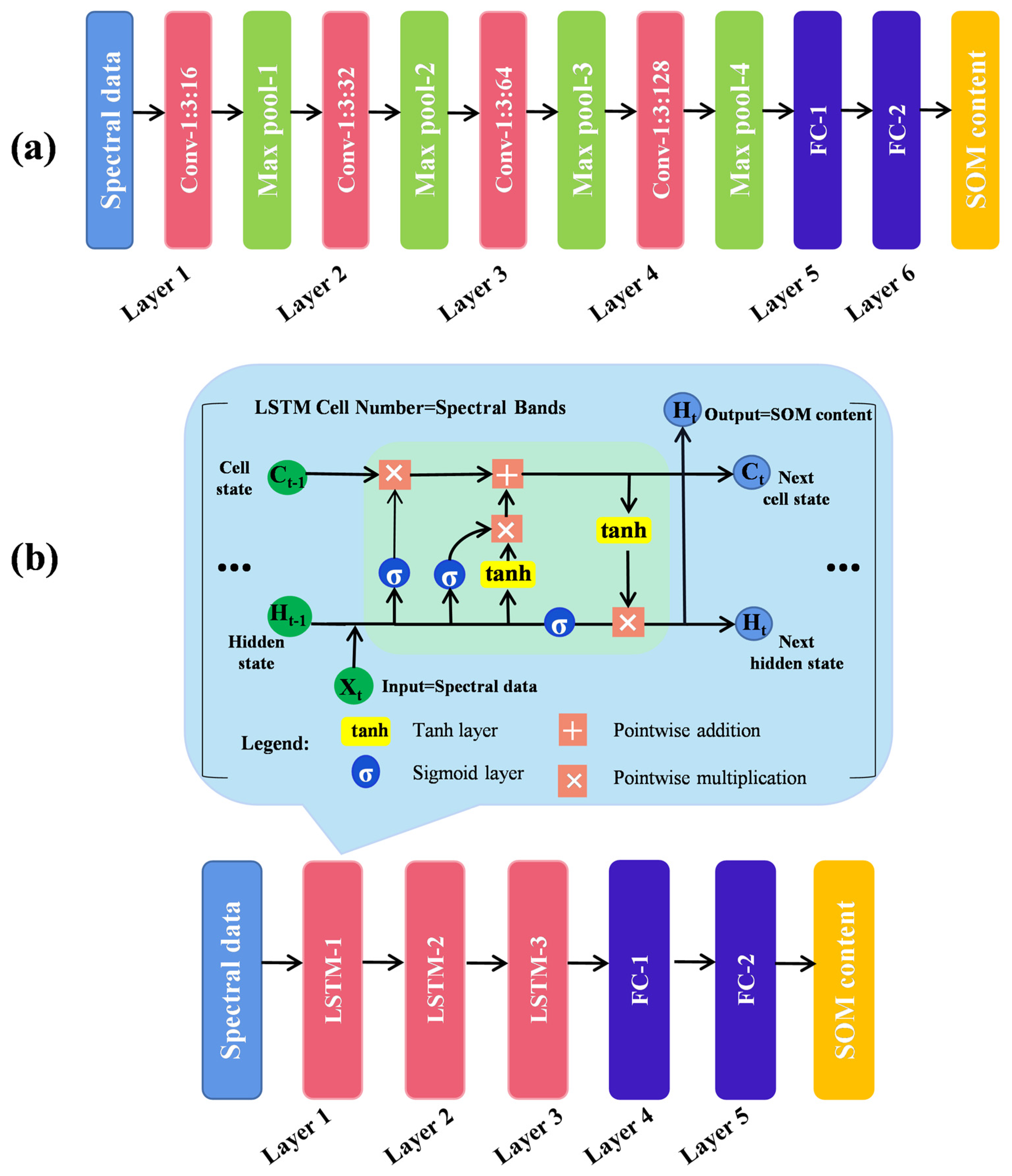
A CNN is a neural network model. CNNs have been used to analyze spectral data. High-level spectral features are extracted by convolutional layers, which are then passed to fully connected layers for the final prediction. Unlike manual selection of the convolution kernel, a CNN learns the convolution kernel automatically through a backpropagation algorithm. This strategy is more suitable for spectral data features. CNNs can capture the correlation between different bands in hyperspectral data through the convolution layer, enabling a better understanding of the spatial structure and features in the data. A Max-Pooling operation is applied after each convolutional layer to reduce the feature dimensionality, retain salient features, and reduce the number of parameters in subsequent convolutional layers [40]. The ReLU activation function was used in this study to reduce the computational complexity, redundancy between parameters, and risk of overfitting. Since the soil spectral reflectance data have only one spectral dimension, a one-dimensional CNN model was chosen for predicting the SOM content. The model structure is shown in Figure 3a. The hyperparameter settings for the model are detailed in Table 2, comprising an input layer, four convolutional layers, four pooling layers, two fully connected layers, and one output layer.
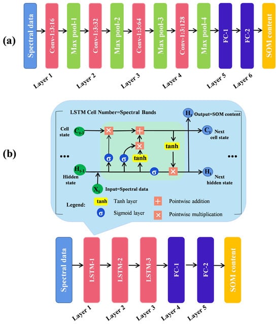
Figure 3.
Schematic diagram of CNN (a) and LSTM (b) network structures.
Table 2.
Hyperparameter settings in CNN.
2.6.3. Long Short-Term Memory (LSTM)
An LSTM model is a type of recurrent neural network (RNN) that is widely used for modeling and prediction using sequential data [41]. Unlike traditional RNNs, LSTMs solve the long-term dependency and gradient vanishing problems by using a gating mechanism. In this study, the LSTM model was employed for predicting SOM content. LSTMs can handle sequential data, such as spectral data, efficiently. A critical component in the LSTM model is the memory cell, which stores and updates information. The memory cell consists of forgetting, input, and output gates, which determine the importance of the spectral data, adjust the memory state, and generate new candidate values through a sigmoid activation function. The Tanh activation function was used for the final prediction of the SOM content. The LSTM model possesses excellent performance for processing sequential data, enabling it to capture the long-term dependencies within the dataset. The structure of the model is shown in Figure 3b. The hyperparameter settings for the model are detailed in Table 3.
Table 3.
Hyperparameter settings in LSTM.
2.7. Model Evaluation
The soil samples were divided into modeling and validation sets using a ratio of 2:1. Subsets of soil types were also divided using the same 2:1 ratio. The RF, CNN, and LSTM models were used to predict the SOM content. Model accuracy was compared using the coefficient of determination (R2), root mean squared error (RMSE), ratio of performance to interquartile distance (RPIQ), and residual prediction deviation (RPD).
3. Results and Analyses
3.1. Descriptive Statistics of SOM Content for Different Grouping Methods
Table 4 presents the descriptive statistics of the SOM content. In the NG strategy, the SOM content of the 1477 samples ranged from 0.37% to 9.81%, with an average content of 4.17% and a skewness value of 0.52%, indicating a non-normal distribution. The skewness (SK) indicated that the SOM content of different soil types deviated from a normal distribution. The CV for the SOM content varied across different soil types, with Arenosols having the highest CV. Arenosols are prone to wind erosion, depending on the location, resulting in significant fluctuations in their SOM content and high CV values. In contrast, Cambisols have a larger range in the SOM content and relatively high CV values. They are commonly found in areas with low topography that are prone to environmental changes, such as soil erosion, affecting soil properties and increasing the variability in the SOM content. Phaeozems had the highest SOM content because of the high humus content, resulting in high water and fertilizer retention. The SG approach was used to classify the samples into six clusters. Significant differences in SOM content were observed among the clusters. Cluster 3 had the highest SOM content and was similar to Phaeozems. Cluster 5 had the lowest SOM content and was similar to Arenosols. The spectral values were high in the range of 400–800 nm due to the presence of iron ions. Cluster 1 was similar to Chernozems. The CV values showed that the data from the three groupings were not normally distributed. For the three different grouping methods, the distribution of organic matter content in both the modeling and validation datasets is illustrated in Figure A3 in Appendix A.
Table 4.
Statistical results of the organic matter content of soil samples.
3.2. One-Dimensional Correlation between FOD Spectral Features and SOM Content
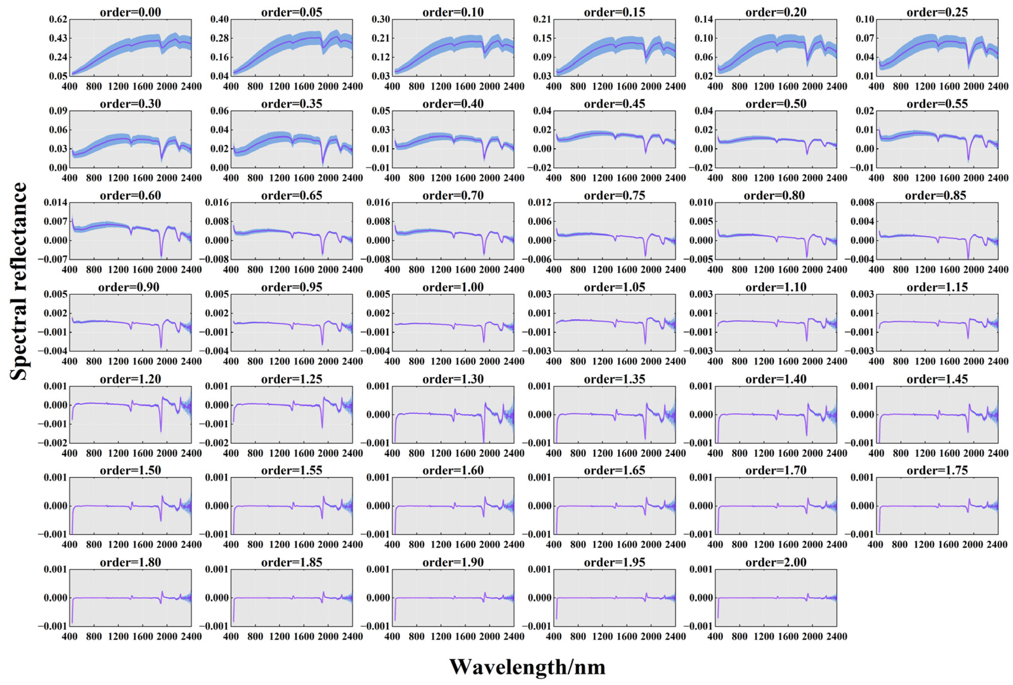
The reflectance curves for different FODs are shown in Figure 4. Order = 0 represents the initial spectral reflectance curve, showing broad absorption bands and apparent differences in spectral characteristics. The results in the blue region indicate differences in spectral characteristics in the northeast region. Consistent with previous studies, the soil spectra showed three moisture absorption bands at 1400 nm, 1900 nm, and 2200 nm. As the order increased from 0 to 1.0, the spectral absorption bands became narrower, and the slope of the curve in the wavelength range of 400–600 nm reached the maximum value of 90°. Small sharp peaks occurred in the 1400–1600 nm range. As the order of the FOD increased from 1 to 1.5, the intensity of the small peaks in the 1400–1600 nm range increased. As the order of the FOD increased from 1.5 to 2, the spectral reflectance remained stable in the range of −0.001 to 0.001, and the absorption valleys of the higher orders were significantly smaller than those of the lower orders. The difference between the other spectra was minimal, nearly 0, indicating that the baseline offset and overlapping peaks were eliminated, the magnitude of the spectral intensities decreased, and the spectral reflectance tended to zero.
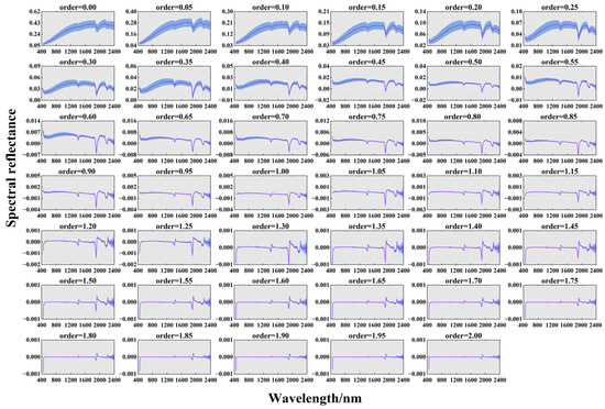
Figure 4.
Spectra of different FODs (range 0–2, interval 0.05). The blue area represents the standard deviation of the spectra.
The one-dimensional Pearson correlation coefficients between the FOD spectra and the SOM content are shown in Figure 5. When the order of the FOD was 0, the RR spectra were negatively correlated with the SOM content, and the correlation was relatively flat in the visible and near-infrared (NIR) bands. The correlation coefficients in the 400–1200 nm range were higher when the order ranged from 0 to 1, and positive correlations were observed at 1400 nm, 1900 nm, and 2200 nm. The number of positive correlations in the NIR region increased as the order increased from 1 to 2.
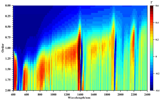
Figure 5.
Correlation coefficient results between SOM and FOD (range 0–2, interval 0.05).
The correlation coefficients between the FOD spectra and the SOM content were more significant in the visible region than in the NIR region. In addition, the correlation was significantly higher for the 1.05th-order spectrum (0.61) than for the other orders (Figure 5 and Table 5). Based on these results, we chose the 1.05th-order derivative spectrum for subsequent analysis and modeling.
Table 5.
Maximum absolute correlation coefficients (MACC) between SOM and FOD spectra.
3.3. Spectral Characteristics of Soil Reflectance
It was found that the spectral noise was more substantial in the ranges of 350–430 nm and 2400–2500 nm. Therefore, the bands in the 430–2400 nm range were selected for subsequent analyses. The spectral reflectance of the soil in the visible bands was affected by organic matter and iron ions, exhibiting notable variation with the increasing wavelength. Significant changes in the spectral reflectance occurred near the 1400, 1900, and 2200 nm bands. This variation is associated with hydroxyl molecules (-OH) in water and clay soils.
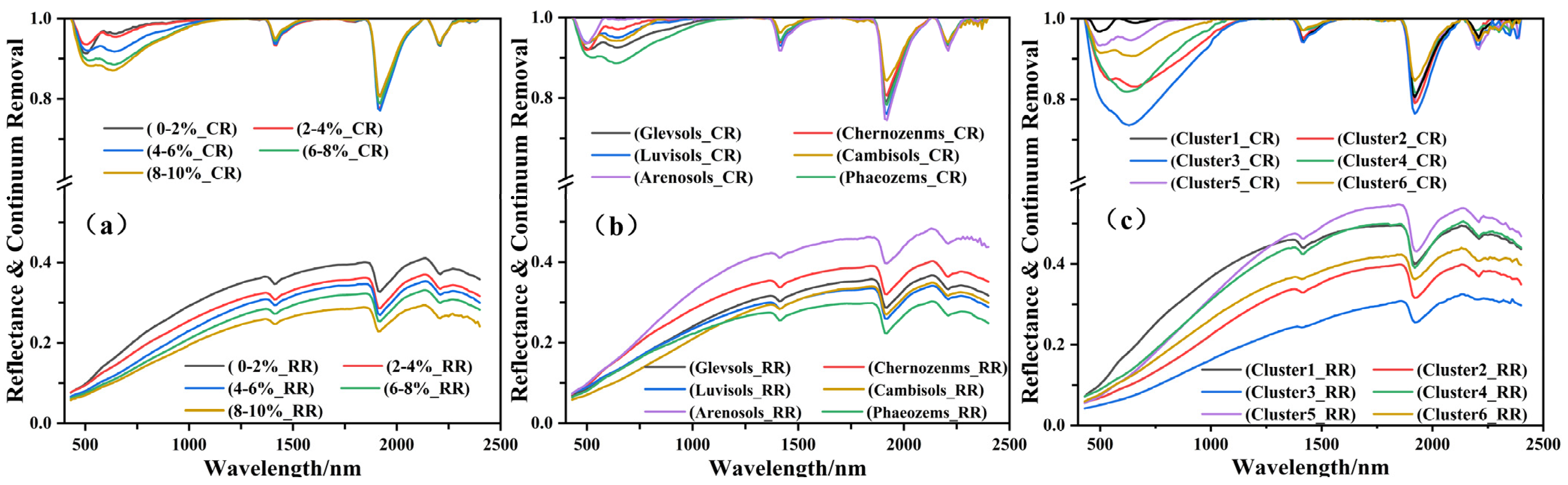
Figure 6a shows that the spectral reflectance profile decreases with an increase in the SOM content, and Figure 6b indicates differences in the spectral reflectance of different soil types. Gleysols exhibited a gradual increase in reflectance across different bands, while Chernozems initially increased and then decreased along the band. Phaeozems decreased at the beginning of the band and then increased. Cambisols were similar to Phaeozems, with a slow increase in reflectance. The reflectance of Arenosols had a higher slope at the beginning of the band and then decreased. The order of the soil types based on the reflectance was Arenosols > Chernozems > Gleysols > Cambisols > Luvisols > Phaeozems, indicating that the reflectance was inversely proportional to the SOM content (see Table 5 for details). New spectral features appeared after CR, significantly increasing the differences between the six soil classes.
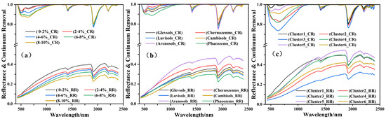
Figure 6.
Soil reflectance spectral curves and envelope removal for (a) no groups, (b) traditional grouping, and (c) spectral grouping.
Figure 6a demonstrates that the shapes of the first two absorption valleys are different, while those of the last three absorption valleys show no significant difference. In addition, as the spectral reflectance increased, the area of the first two absorption valleys increased. The first two absorption valleys of the different soil types were significantly different (Figure 6b). The higher the SOM content, the larger the area and depth of the first absorption valley (V1), and the lower the SOM content, the more anterior the position of V1. The lowest points of V1 and V2 of the Phaeozems corresponded to the lowest CR values, and the area of the second absorption valley (A2) was larger than that of the first absorption valley (A1). In contrast, Chernozems and Luvisols had higher CR values for V1 and V2, and A1 > A2. In contrast to Phaeozems, Arenosols had symmetrically shaped and narrower V1s. Gleysols had wider V2 than V1, and A2 > A1. Cambisols had a larger A1 and A2, and A1 > A2. In addition, the slope (S5) between V1 and V2 was negative in most cases. The order of the soil types based on the CR values was Gleysols > Arenosols > Chernozems > Luvisols > Cambisols > Phaeozems, suggesting an inverse relationship between the SOM content and the CR values.
K-means clustering was employed to classify the soil samples into six clusters. The spectral differences between the clusters were related to the SOM content. Cluster 1 was similar to Chernozems; the second absorption valley was slightly wider than the first, and A1 > A2. Cluster 3 was similar to Phaeozems, with the lowest reflectance value. The lowest point of the absorption valley corresponded to the highest CR value and the highest SOM content (5.81%). Cluster 5 was similar to Arenosols, with the highest reflectance value and the lowest SOM content (2.09%). The first absorption valley was symmetric, and A1 > A2. The other clusters had distinctive features in the post-CR curves, e.g., A2 was much larger than A1 in Cluster 2 and Cluster 6.
3.4. Spectral Variable Selection
Variable selection is critical for optimizing models and interpreting multivariate regression analysis. Selecting the most informative variables and eliminating highly correlated variables reduces redundant information and model complexity. During variable selection, interactions and covariances must be considered to ensure the model’s high predictive power and interpretability.
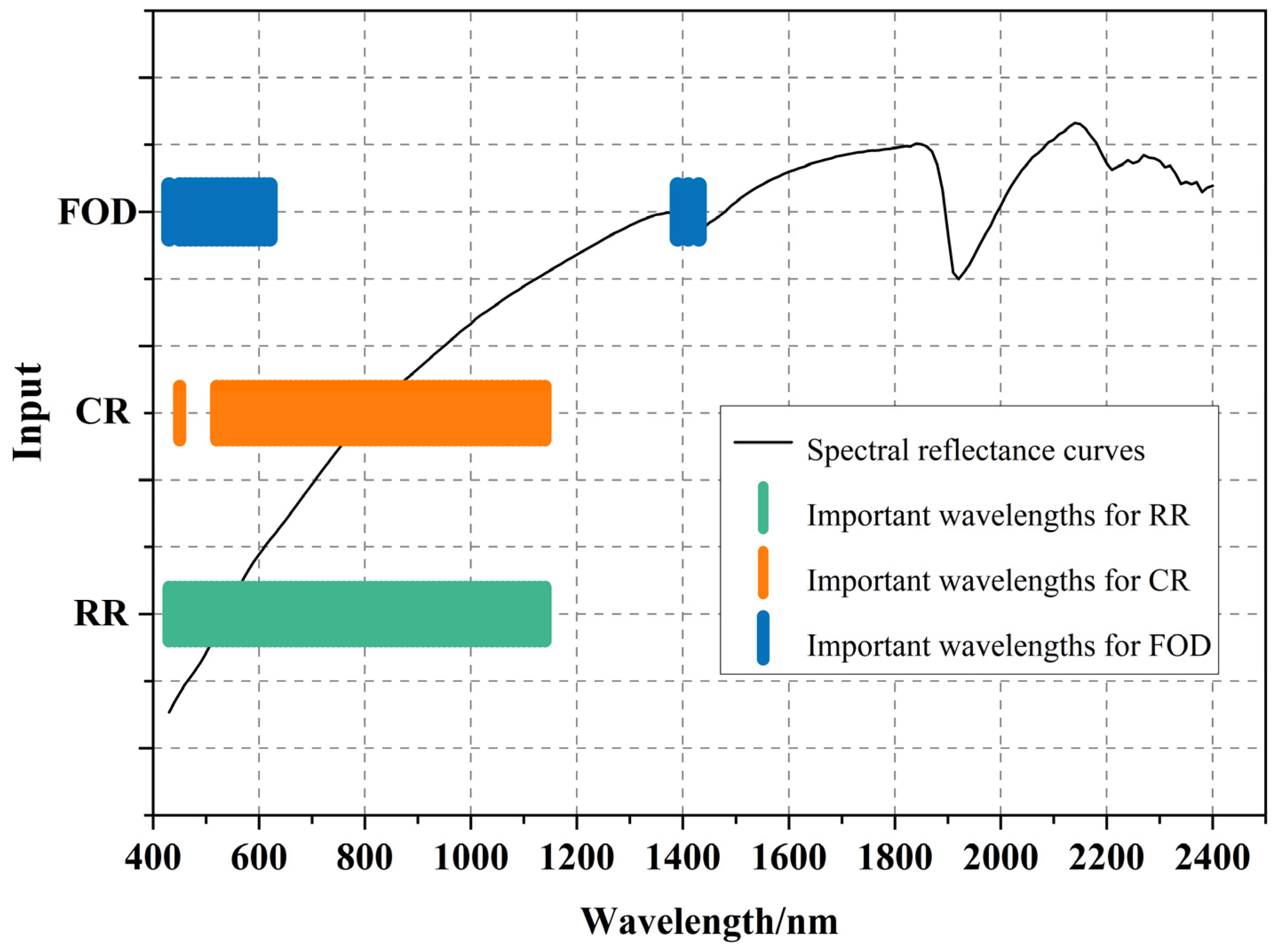
As shown in Figure 7, the selected input variables cover the range of 400–2400 nm. We used a correlation coefficient threshold of |r| > 0.5 and selected 72, 53, and 22 variables for the RR, CR, and FOD inputs, representing 36%, 27%, and 11% of the total input variables, respectively. The FOD at 1390 nm and 1400 nm was positively correlated with the SOM content. We selected DPL2, A2, A1 + A2, K5, and W2 as the optimal feature parameters of the SCPs. Most indicators were situated in the 600–800 nm range, consistent with the range where the SOM content exhibited a high correlation with the variables. DPL2 and K5 were negatively correlated with the SOM content. For the TG of the the different soil classes, DPL2 and A1 + A2 increased, and K5 decreased with the increasing SOM content.
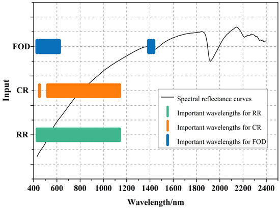
Figure 7.
Distribution of important SOM bands under different input conditions. (The three colors in the figure represent the ranges covered by sensor bands based on FOD, CR, and RR, respectively. The curves represent the spectral reflectance curves after S-G smoothing.)
3.5. Model Performance and Evaluation
The SOM prediction results differed for different modeling methods. As shown in Table 6, the accuracy of the deep learning LSTM model was higher than that of the RF and CNN models. The optimal model had R2 = 0.82, RMSE = 0.69, RPIQ = 2.62, and RPD = 2.07. LSTM uses a convolutional layer to extract deep nonlinear features, improving the model’s prediction ability. The ranking of the grouping methods based on the prediction accuracy was SG > TG > NG. The correlation between the SOM content and the inputs of the subgroups significantly increased after grouping, indicating that grouping improves prediction accuracy. CR, FOD, and SCPs improved the model’s prediction accuracy for different grouping approaches and different inputs.
Table 6.
SOM prediction results for different models, different grouping methods, and different inputs.
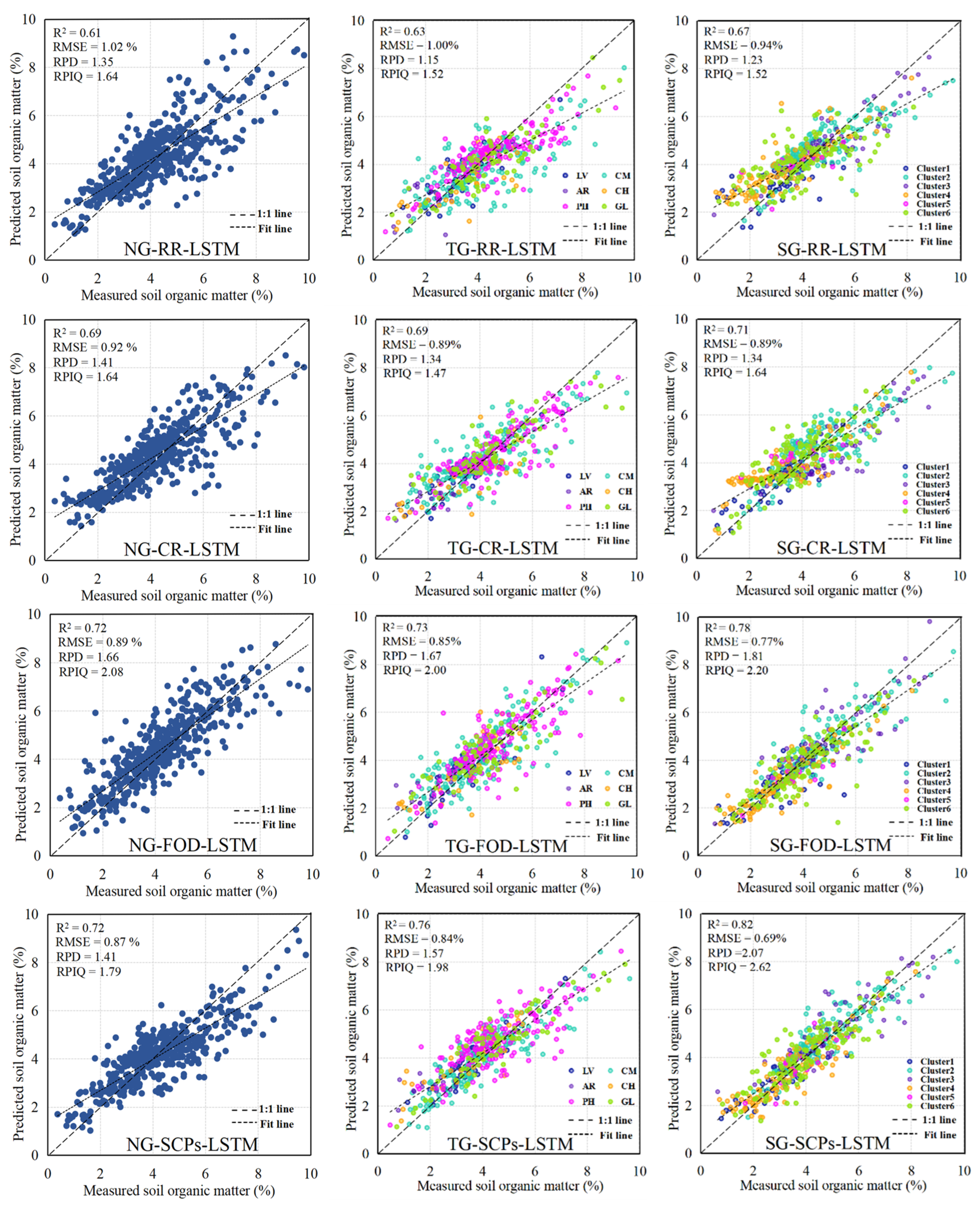
Figure 8 shows the scatterplot between the measured and predicted SOM contents. When CR and SCPs are used as inputs into the LSTM model, the SOM values are closer to the 1:1 line, indicating a closer alignment between predicted and measured values. The CNN model has a lower R2 value than the LSTM model. The model accuracy is higher for the RF than the other three inputs when SCPs are used as input, consistent with the results of a previous study [11]. Continuous inputs into deep learning models result in higher prediction accuracy (scatter plots of the CNN model and RF model based on the three grouping methods and four inputs are shown in Figure A1 and Figure A2 in Appendix A).
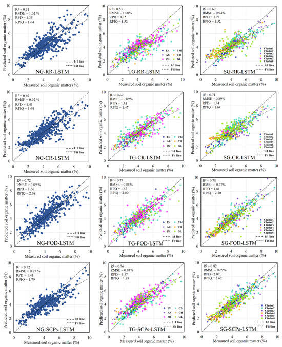
Figure 8.
Scatterplot of SOM content for LSTM model based on three grouping methods and four inputs.
4. Discussion
This study differs from others predicting SOM content by employing an integrated approach. Unlike studies focusing on a single factor (e.g., grouping method, number of inputs, or prediction model), we considered all three critical elements to address the complexity of SOM content prediction for large-scale farmland. Due to the heterogeneity of SOM, an optimal combination of the grouping method, input volume, and prediction model is required for predicting the SOM content in large regions due to the SOM heterogeneity. The LSTM model precisely captured the relationship between the SOM content and the spectral features; thus, it was the most suitable prediction algorithm for the SOM content in this study. We identified significant differences in the spectral features of different soil types. Therefore, we used SG combined with the K-means method to cluster the spectral features of different soil classes. This approach strengthened our study by providing a more accurate classification of different soil samples. We provide here an in-depth discussion on the impact of several key factors on SOM content prediction, practical recommendations for selecting deep learning models and hyperspectral data, and the limitations of this study.
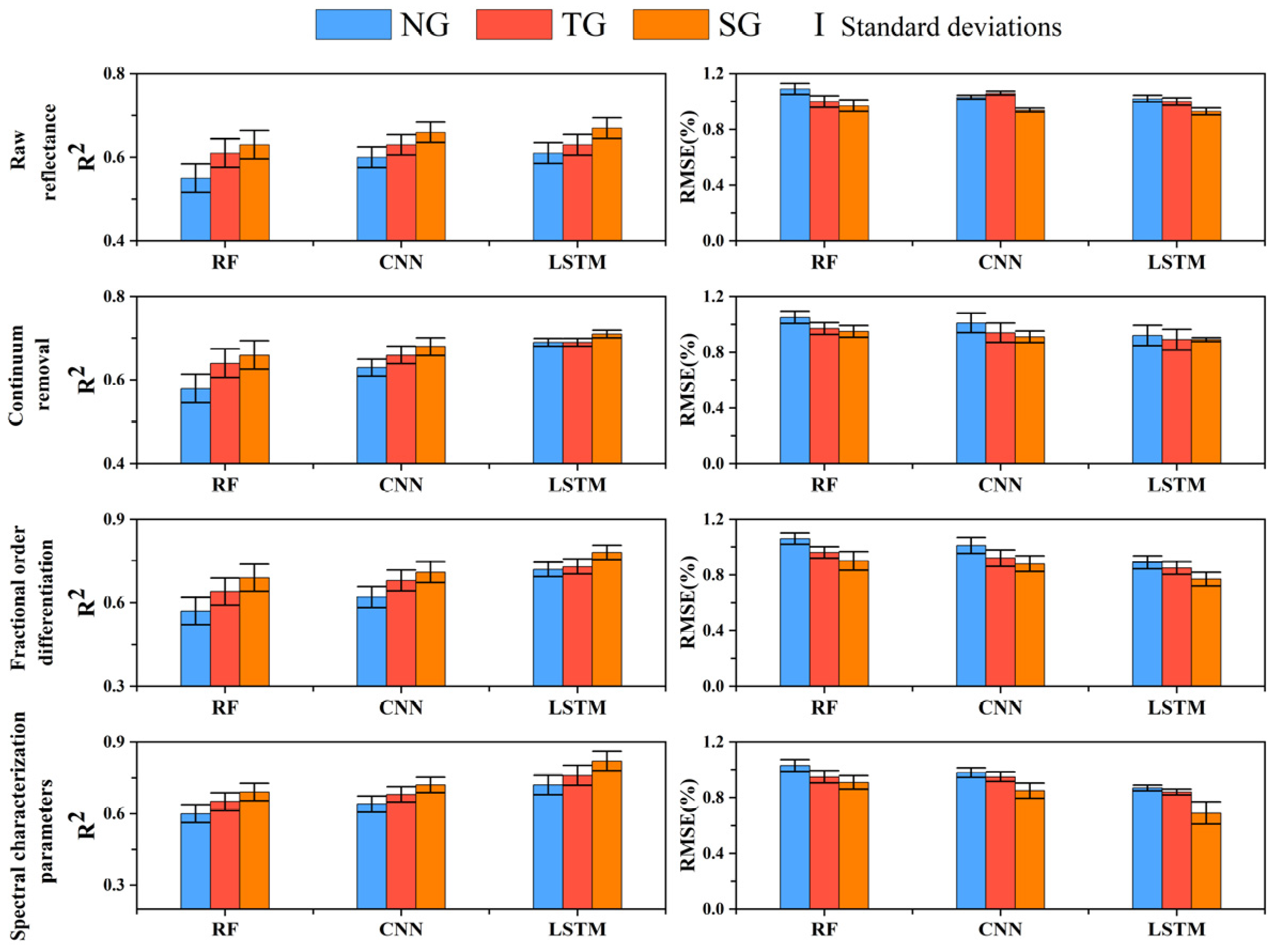
4.1. Impact of Deep Learning on the Performance of SOM Content Prediction Models
The comprehensive comparison of three different algorithms indicates that LSTM and CNN models outperform RF models in predicting SOM content. Our approach demonstrates flexibility in adapting to hyperspectral data and provides high performance (Figure 9). The LSTM model, as a type of recurrent neural network with memory functionality, swiftly captures intricate nonlinear relationships and exhibits robust modeling capabilities for continuous data. Consequently, as depicted in Figure 9, in this study, the accuracy of LSTM in predicting SOM content surpasses the other two models, with an R2 of approximately 0.82, an RMSE of about 0.69%, a PRIQ of around 2.62, and an RPD of approximately 2.07. In comparison to RF, CNN and LSTM are more adept at considering sequential features, thereby enhancing model robustness and reducing errors. For preprocessing hyperspectral data, we observed that spectral feature parameters significantly improve deep learning models. Machine learning algorithms, such as RF, coupled with 1.05-order FOD spectral preprocessing, can extract spectral features and achieve performance levels similar to deep learning models. Overall, the LSTM model performs the best, followed by CNN, and RF ranks last. LSTM is suitable for spectral data with limited wavelength inputs, while CNN is effective for features such as hyperspectral reflectance.
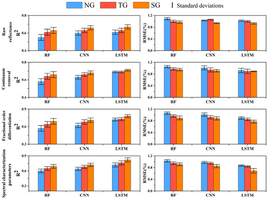
Figure 9.
Comparison of SOM prediction performance (error bars represent the standard deviation of model simulation performance).
In addition, we observed that the performance of the hyperspectral reflectance data did not significantly improve the performance of the LSTM and CNN models. These two highly nonlinear deep learning models already have strong feature learning capabilities and can fit the relationship between the spectral features and the SOM content without much preprocessing. Meanwhile, the performance of the RF model was significantly improved by spectral preprocessing, especially when the FOD was used as the input.
The LSTM model’s uncertainty was evaluated by calculating the relative absolute error (RAE) and dividing the SOM content into five intervals (Figure 10). The model’s RAE was significantly correlated with the SOM content. The LSTM model had high prediction errors at low (0–2%) and high (8–10%) SOM contents, with lower prediction errors observed at intermediate contents (2–8%).
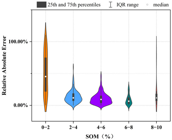
Figure 10.
LSTM model uncertainty analysis. (The x-axis denotes the SOM range intervals, and the y-axis represents the relative absolute error. The violin shapes depict the distribution of the data. In the violin plot, the black bars correspond to the 25th and 75th percentiles. The white dots on the black bars indicate the median.)
4.2. Comparison of Grouping Methods and Inputs
Guerrero et al. [42] found that local regression was superior to global regression. In this study, three groupings (NG, TG, and SG) and four input variables (RR, CR, FOD, and SCPs) were selected. Consistent with previous studies [43], local regression resulted in a higher accuracy in SOM prediction compared to the NG method, confirming the significance of soil grouping for SOM prediction in large areas.
The rationales of the different methods resulted in differences in the number of variables and locations. The results showed that variable selection helped to reduce model complexity by eliminating redundant variables and retaining only those significantly correlated with the SOM content. The methods based on the four inputs had higher accuracy than the model using all bands. The SOM prediction performance is related to the spectral preprocessing method [9,44]. It has been shown that mathematical methods for resampling the spectral curves and enhancing the linearity of the spectral features improved prediction accuracy. For example, spectral reflectance curves are subjected to derivative operations using mathematical transformations, such as first-order differentiation, logarithmic, and inverse transformations [45], or CR to amplify the local absorption features of the spectral curves [46]. However, these methods have limitations, i.e., mathematical transformations may increase the noise level [47]. The number of bands remains the same after mathematical transformations; therefore, dimensionality reduction techniques such as principal component analysis (PCA) or competitive adaptive reweighting (CARS) can be considered [48,49]. Limiting the spectral range to 400–1200 nm resulted in higher correlations between the spectral features and the SOM content [50].
The TG resulted in significantly higher prediction accuracy of the SOM content than NG (Figure 8); i.e., the R2 was 0.21 higher, the RMSE was 25% lower, the RPIQ was 0.67 higher, and the RPD was 0.45 higher. The reason for this is that the soil samples were obtained from multiple soil types. Due to differences in the soil parent material and soil structure, the spectral characteristics differed for different soil types, affecting the prediction accuracy. The spectral differences among the soil classes were lower after TG. For instance, the first two absorption valleys of different soil classes were dissimilar after CR. The first two absorption valleys of the Phaeozems were profound, with the second one being larger than the first one. In contrast, the first absorption valley of the Arenosols was symmetric, and the second one was smaller. Thus, SG improved the accuracy of SOM prediction.
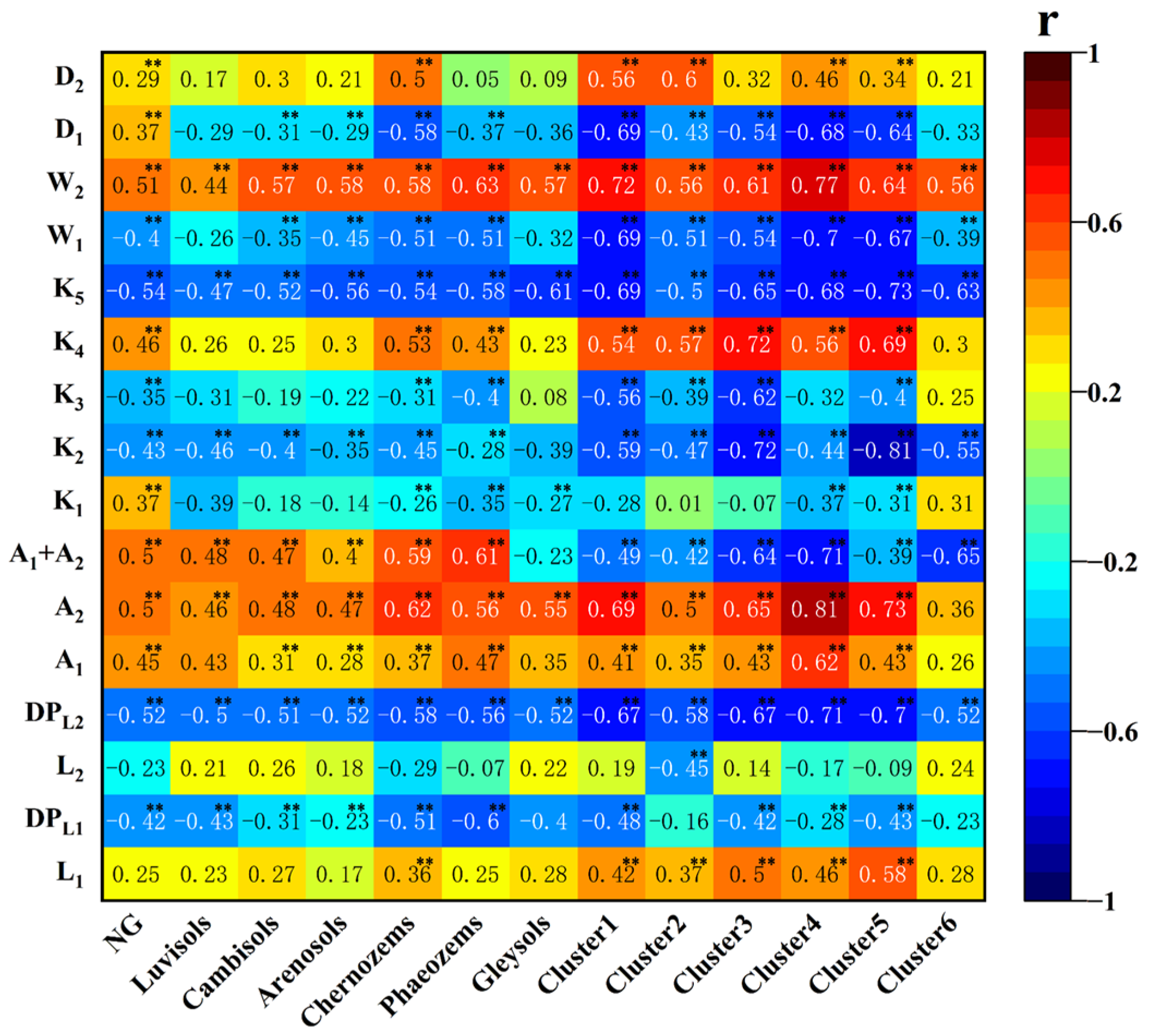
We found that the model with SG and taking the SCPs as input variables performed the best and provided the highest accuracy. SCPs are indicators of soil chemical and physicochemical properties and are highly informative for predicting the SOM content. They were generally highly correlated with the SOM content (Figure 11). DPL2, A2, A1 + A2, K5, and W2 had the highest correlations. The correlation was higher between SCPs and the SOM content of Phaeozems when TG was used as a grouping method, with a W2 of 0.63. Only DPL2 exceeded 0.5 for Luvisols. For SG, Cluster 4 had the highest correlation, with an A2 of 0.81. Except for Clusters 2 and 6, all other clusters had correlation coefficients exceeding 0.7. These significant correlations indicate that the spectral features were extracted more efficiently using SG to improve the model’s generalization ability. FOD improved the SOM prediction accuracy by capturing the features of the first two absorption valleys of the spectral curves after CR. CR and FOD performed comparably as input variables in terms of prediction accuracy.

Figure 11.
Correlation between SCPs and SOM content for subsets of different grouping methods. (Significance at the p < 0.01 level **).
4.3. Research Limitations
The results of this study showed that the combination of SG, SCPs, and the deep learning LSTM algorithm was the most effective method for predicting SOM content in Northeast China. Although deep learning has high accuracy, it is challenging to determine the optimal parameters quickly due to the complex network structure [51,52]. Therefore, more efficient parameter optimization methods, such as stochastic search or Bayesian optimization, must be considered to optimize model performance. In addition, dropout layers or other activation functions can be incorporated to improve model performance [53]. The training data for the model were soil data from the northeast region of China. However, the model’s generalization performance should be validated in other regions, as soil properties and environmental conditions in different regions may impact its applicability. Other factors, such as soil moisture, texture, and soil parent material, must be considered when applying the model to other regions. Although several methods and algorithms were used in this study for SOM content prediction, the results have uncertainty. Therefore, the confidence interval or error range should be considered in practical applications. This paper considered only spectral features in the visible, NIR, and shortwave infrared bands. The mid-infrared and thermal infrared bands could be assessed in future studies, expanding the spectral measurement range. In addition, future research could consider optimizing inputs, selecting different algorithms, and considering more uncertainties for SOM prediction.
5. Conclusions
This study evaluated the potential of combining different algorithms, grouping methods, and inputs for SOM prediction using hyperspectral reflectance data from 1477 surface soil samples in Northeastern China. The algorithms included RF, CNN, and LSTM models, with the grouping methods comprising NG, TG, and SG and the inputs including RR, CR, FOD, and SCPs. The study revealed that the LSTM model with SG and SCP inputs obtained the highest prediction accuracy. The LSTM model extracted the deep relationships between the spectral data and the SOM content. SG reduced the variability in the spectral features among different soil classes, and the SCPs reflected the absorption features of the spectral curves so that different soil samples could be distinguished accurately. This combination provided the most accurate results for soil property assessment. The ranking of the models for SOM content prediction was LSTM > CNN > RF, and the ranking of the grouping approach was SG > TG > NG. When SCPs were used as inputs, the RMSE was 0.24%, 0.20%, and 0.08% lower, and the R2 was 0.15, 0.11, and 0.04 higher, respectively, than for the other models. This study also identified the optimum SCPs (DPL2, A2, A1 + A2, and W2) for SOM content prediction. However, the predictive ability of the LSTM model varied for different SOM content ranges. Small errors were observed at intermediate SOM contents (2–8%), whereas relatively large errors occurred at low (0–2%) and high (8–10%) contents. This discrepancy was attributed to the model’s ability to learn the data distribution for different content ranges. Further research is required to optimize the model’s performance. The deep learning model mined the relationship between spectral features and SOM content using different grouping methods and inputs, achieving high-precision SOM content prediction in a large area. The study results strongly support the improvement in large-scale SOM content prediction accuracy and reduction in spatial heterogeneity in large regions, and offer scientific methods and foundations for the future prediction of SOM content snapshots.
Author Contributions
Conceptualization, X.Z.; Data curation, C.D. and C.L.; Formal analysis, C.L., X.M. and C.D.; Methodology, X.Z., X.M. and C.D.; Project administration, X.Z. and H.L.; Software, Y.H. and H.A.; Writing—original draft, C.D.; Writing—review and editing, H.L. All authors have read and agreed to the published version of the manuscript.
Funding
This research was supported by the Project of Introducing Talents of Jilin Agricultural University (202020010), the Jilin Provincial Development and Reform Commission Innovation Capacity Building Project (2021C044-10), and the National Key R&D Program of China (2021YFD1500100).
Data Availability Statement
The data presented in this study is available upon request by contacting the corresponding author. Due to copyright restrictions, the data from this study is not publicly disclosed.
Acknowledgments
We appreciate the financial support provided by the Talent Introduction Project of Jilin Agricultural University (202020010), the Innovation Capability Building Project of the Jilin Provincial Development and Reform Commission (2021C044-10), and the National Key Research and Development Program (2021YFD1500100). All authors express gratitude for the valuable comments and suggestions provided by the editors and anonymous reviewers.
Conflicts of Interest
The authors declare no conflicts of interest.
Appendix A
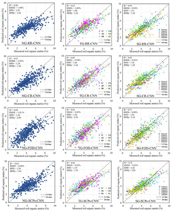
Figure A1.
Scatterplots between measured and predicted SOM content for the CNN model with three grouping methods and four inputs.
Figure A1.
Scatterplots between measured and predicted SOM content for the CNN model with three grouping methods and four inputs.
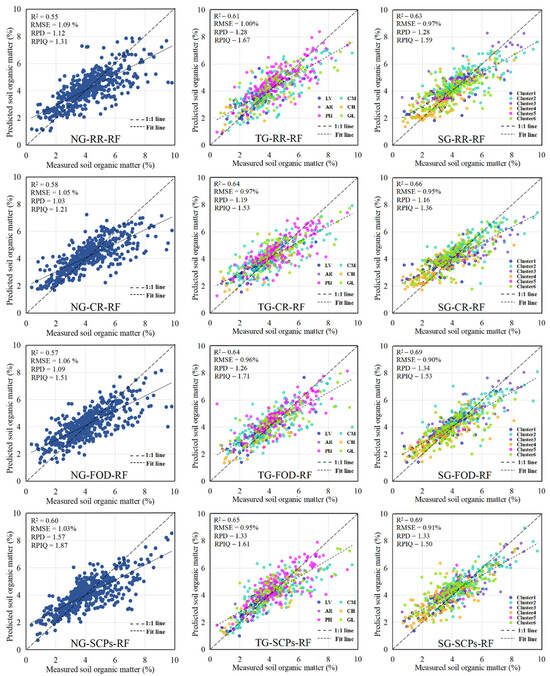
Figure A2.
Scatterplots between measured and predicted SOM content for the RF model with three grouping methods and four inputs.
Figure A2.
Scatterplots between measured and predicted SOM content for the RF model with three grouping methods and four inputs.
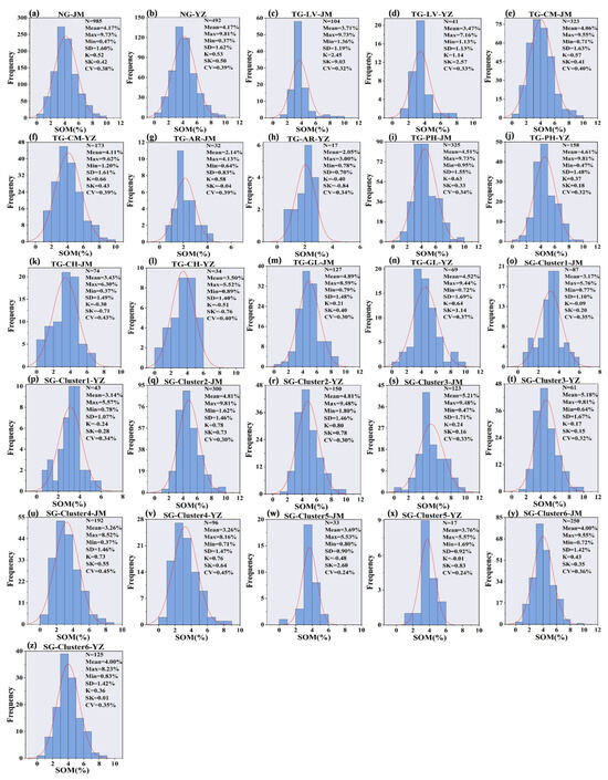
Figure A3.
Descriptive statistics and histograms of the distribution of soil organic matter (SOM) content in % for the modeling and validation sets. (a,b) Based on the NG—no groups; (c–n) Based on TG—traditional grouping; (o–z) Based on SG—spectral grouping. LV, CM, AR, CH, PH, and GL in TG denote Luvisols, Cambisols, Arenosols, Chernozems, Phaeozems, and Gleysols. Clusters 1–6 in SG denote the clustering grouping based on K-means clustering. N—number of samples; Mean—mean value %; Max—maximum %; Min—minimum %; SD—standard deviation %; K—kurtosis; SK—skewness; CV—coefficient of variation %; JM—modeling set; YZ—validation set.
References
- Ge, X.; Ding, J.; Jin, X.; Wang, J.; Chen, X.; Li, X.; Liu, J.; Xie, B. Estimating Agricultural Soil Moisture Content through UAV-Based Hyperspectral Images in the Arid Region. Remote Sens. 2021, 13, 1562. [Google Scholar] [CrossRef]
- Rossel, R.V.; Behrens, T.; Ben-Dor, E.; Brown, D.J.; Demattê, J.A.M.; Shepherd, K.D.; Shi, Z.; Stenberg, B.; Stevens, A.; Adamchuk, V. A Global Spectral Library to Characterize the World’s Soil. Earth-Sci. Rev. 2016, 155, 198–230. [Google Scholar] [CrossRef]
- Belyaev, B.I.; Belyaev, Y.V.; Katkovskii, L.V.; Tsikman, I.M. Estimation and Analysis of the Parameters of a Field Spectroradiometer Covering the Spectral Range 350–2500 Nm. J. Appl. Spectrosc. 2009, 76, 577–584. [Google Scholar] [CrossRef]
- Nocita, M.; Stevens, A.; van Wesemael, B.; Aitkenhead, M.; Bachmann, M.; Barthès, B.; Ben Dor, E.; Brown, D.J.; Clairotte, M.; Csorba, A.; et al. Chapter Four—Soil Spectroscopy: An Alternative to Wet Chemistry for Soil Monitoring. In Advances in Agronomy; Sparks, D.L., Ed.; Academic Press: Cambridge, MA, USA, 2015; Volume 132, pp. 139–159. [Google Scholar]
- Clark, R.N.; King, T.V.V.; Klejwa, M.; Swayze, G.A.; Vergo, N. High Spectral Resolution Reflectance Spectroscopy of Minerals. J. Geophys. Res. Solid Earth 1990, 95, 12653–12680. [Google Scholar] [CrossRef]
- Sanderman, J.; Baldock, J.A.; Dangal, S.R.S.; Ludwig, S.; Potter, S.; Rivard, C.; Savage, K. Soil Organic Carbon Fractions in the Great Plains of the United States: An Application of Mid-Infrared Spectroscopy. Biogeochemistry 2021, 156, 97–114. [Google Scholar] [CrossRef]
- Röder, L.L.; Fischer, H. Theoretical Investigation of Applicability and Limitations of Advanced Noise Reduction Methods for Wavelength Modulation Spectroscopy. Appl. Phys. B 2022, 128, 10. [Google Scholar] [CrossRef]
- Gholizadeh, A.; Bor\uuvka, L.; Saberioon, M.M.; Kozák, J.; Vašát, R.; Němeček, K. Comparing Different Data Preprocessing Methods for Monitoring Soil Heavy Metals Based on Soil Spectral Features. Soil Water Res. 2015, 10, 218–227. [Google Scholar] [CrossRef]
- Bian, X. Spectral Preprocessing Methods. In Chemometric Methods in Analytical Spectroscopy Technology; Chu, X., Huang, Y., Yun, Y.-H., Bian, X., Eds.; Springer Nature: Singapore, 2022; pp. 111–168. ISBN 978-981-19162-5-0. [Google Scholar]
- Malenovskỳ, Z.; Homolová, L.; Zurita-Milla, R.; Lukeš, P.; Kaplan, V.; Hanuš, J.; Gastellu-Etchegorry, J.-P.; Schaepman, M.E. Retrieval of Spruce Leaf Chlorophyll Content from Airborne Image Data Using Continuum Removal and Radiative Transfer. Remote Sens. Environ. 2013, 131, 85–102. [Google Scholar] [CrossRef]
- Meng, X.; Bao, Y.; Zhang, X.; Wang, X.; Liu, H. Prediction of Soil Organic Matter Using Different Soil Classification Hierarchical Level Stratification Strategies and Spectral Characteristic Parameters. Geoderma 2022, 411, 115696. [Google Scholar] [CrossRef]
- Bayer, A.; Bachmann, M.; Müller, A.; Kaufmann, H. A Comparison of Feature-Based MLR and PLS Regression Techniques for the Prediction of Three Soil Constituents in a Degraded South African Ecosystem. Appl. Environ. Soil Sci. 2012, 2012, e971252. [Google Scholar] [CrossRef]
- Laukamp, C.; Rodger, A.; LeGras, M.; Lampinen, H.; Lau, I.C.; Pejcic, B.; Stromberg, J.; Francis, N.; Ramanaidou, E. Mineral Physicochemistry Underlying Feature-Based Extraction of Mineral Abundance and Composition from Shortwave, Mid and Thermal Infrared Reflectance Spectra. Minerals 2021, 11, 347. [Google Scholar] [CrossRef]
- Qiao, X.-X.; Wang, C.; Feng, M.-C.; Yang, W.-D.; Ding, G.-W.; Sun, H.; Liang, Z.-Y.; Shi, C.-C. Hyperspectral Estimation of Soil Organic Matter Based on Different Spectral Preprocessing Techniques. Spectrosc. Lett. 2017, 50, 156–163. [Google Scholar] [CrossRef]
- Hong, Y.; Chen, S.; Liu, Y.; Zhang, Y.; Yu, L.; Chen, Y.; Liu, Y.; Cheng, H.; Liu, Y. Combination of Fractional Order Derivative and Memory-Based Learning Algorithm to Improve the Estimation Accuracy of Soil Organic Matter by Visible and near-Infrared Spectroscopy. Catena 2019, 174, 104–116. [Google Scholar] [CrossRef]
- Stenberg, B.; Viscarra Rossel, R.A.; Mouazen, A.M.; Wetterlind, J. Chapter Five—Visible and Near Infrared Spectroscopy in Soil Science. In Advances in Agronomy; Sparks, D.L., Ed.; Academic Press: Cambridge, MA, USA, 2010; Volume 107, pp. 163–215. [Google Scholar]
- Shi, Y.; Zhao, J.; Song, X.; Qin, Z.; Wu, L.; Wang, H.; Tang, J. Hyperspectral Band Selection and Modeling of Soil Organic Matter Content in a Forest Using the Ranger Algorithm. PLoS ONE 2021, 16, e0253385. [Google Scholar] [CrossRef]
- Jaconi, A.; Don, A.; Freibauer, A. Prediction of Soil Organic Carbon at the Country Scale: Stratification Strategies for near-Infrared Data. Eur. J. Soil Sci. 2017, 68, 919–929. [Google Scholar] [CrossRef]
- Genot, V.; Colinet, G.; Bock, L.; Vanvyve, D.; Reusen, Y.; Dardenne, P. Near Infrared Reflectance Spectroscopy for Estimating Soil Characteristics Valuable in the Diagnosis of Soil Fertility. J. Infrared Spectrosc. 2011, 19, 117–138. [Google Scholar] [CrossRef]
- Xu, M.; Chu, X.; Fu, Y.; Wang, C.; Wu, S. Improving the Accuracy of Soil Organic Carbon Content Prediction Based on Visible and Near-Infrared Spectroscopy and Machine Learning. Environ. Earth Sci. 2021, 80, 326. [Google Scholar] [CrossRef]
- Gogé, F.; Joffre, R.; Jolivet, C.; Ross, I.; Ranjard, L. Optimization Criteria in Sample Selection Step of Local Regression for Quantitative Analysis of Large Soil NIRS Database. Chemom. Intell. Lab. Syst. 2012, 110, 168–176. [Google Scholar] [CrossRef]
- Sun, W.; Zhang, X.; Zou, B.; Wu, T. Exploring the Potential of Spectral Classification in Estimation of Soil Contaminant Elements. Remote Sens. 2017, 9, 632. [Google Scholar] [CrossRef]
- Ramirez-Lopez, L.; Behrens, T.; Schmidt, K.; Stevens, A.; Demattê, J.A.M.; Scholten, T. The Spectrum-Based Learner: A New Local Approach for Modeling Soil Vis–NIR Spectra of Complex Datasets. Geoderma 2013, 195–196, 268–279. [Google Scholar] [CrossRef]
- Xu, Z.; Zhao, X.; Guo, X.; Guo, J. Deep Learning Application for Predicting Soil Organic Matter Content by VIS-NIR Spectroscopy. Comput. Intell. Neurosci. 2019, 2019, 1–11. [Google Scholar] [CrossRef]
- Zhang, L.; Cai, Y.; Huang, H.; Li, A.; Yang, L.; Zhou, C. A CNN-LSTM Model for Soil Organic Carbon Content Prediction with Long Time Series of MODIS-Based Phenological Variables. Remote Sens. 2022, 14, 4441. [Google Scholar] [CrossRef]
- Wadoux, A.M.J.-C.; Padarian, J.; Minasny, B. Multi-Source Data Integration for Soil Mapping Using Deep Learning. Soil 2019, 5, 107–119. [Google Scholar] [CrossRef]
- Ng, W.; Minasny, B.; de Sousa Mendes, W.; Demattê, J.A.M. The Influence of Training Sample Size on the Accuracy of Deep Learning Models for the Prediction of Soil Properties with Near-Infrared Spectroscopy Data. Soil 2020, 6, 565–578. [Google Scholar] [CrossRef]
- Nelson, D.W.; Sommers, L.E. A Rapid and Accurate Procedure for Estimation of Organic Carbon in Soils. Proc. Indiana Acad. Sci. 1974, 84, 456–462. [Google Scholar]
- Pribyl, D.W. A Critical Review of the Conventional SOC to SOM Conversion Factor. Geoderma 2010, 156, 75–83. [Google Scholar] [CrossRef]
- Bao, Y.; Meng, X.; Ustin, S.; Wang, X.; Zhang, X.; Liu, H.; Tang, H. Vis-SWIR Spectral Prediction Model for Soil Organic Matter with Different Grouping Strategies. Catena 2020, 195, 104703. [Google Scholar] [CrossRef]
- Delwiche, S.R.; Reeves, J.B. A Graphical Method to Evaluate Spectral Preprocessing in Multivariate Regression Calibrations: Example with Savitzky–Golay Filters and Partial Least Squares Regression. Appl. Spectrosc. 2010, 64, 73–82. [Google Scholar] [CrossRef]
- Savitzky, A.; Golay, M.J.E. Smoothing and Differentiation of Data by Simplified Least Squares Procedures. Anal. Chem. 1964, 36, 1627–1639. [Google Scholar] [CrossRef]
- Ting, H. Study on Spectral Features of Soil Fe2O3. Geogr. Geo-Inf. Sci. 2006. [Google Scholar] [CrossRef]
- Santos, M.J.; Hestir, E.L.; Khanna, S.; Ustin, S.L. Image Spectroscopy and Stable Isotopes Elucidate Functional Dissimilarity between Native and Nonnative Plant Species in the Aquatic Environment. New Phytol. 2012, 193, 683–695. [Google Scholar] [CrossRef]
- Zhang, Y.; Li, M.; Zheng, L.; Zhao, Y.; Pei, X. Soil Nitrogen Content Forecasting Based on Real-Time NIR Spectroscopy. Comput. Electron. Agric. 2016, 124, 29–36. [Google Scholar] [CrossRef]
- Zhang, W.L.; Xu, A.G.; Zhang, R.L.; Ji, H.J.; Wu, S.X. Review of Soil Classification and Revision of China Soil Classification System. Sci. Agric. Sin. 2014, 47, 3214–3230. [Google Scholar]
- Shang, X.; Li, X.; Morales-Esteban, A.; Asencio-Cortés, G.; Wang, Z. Data Field-Based K-Means Clustering for Spatio-Temporal Seismicity Analysis and Hazard Assessment. Remote Sens. 2018, 10, 461. [Google Scholar] [CrossRef]
- Chen, X.; Li, H.; Zhang, S.; Chen, Y.; Fan, Q. High Spatial Resolution PM2.5 Retrieval Using MODIS and Ground Observation Station Data Based on Ensemble Random Forest. IEEE Access 2019, 7, 44416–44430. [Google Scholar] [CrossRef]
- Díaz-Uriarte, R.; Alvarez de Andrés, S. Gene Selection and Classification of Microarray Data Using Random Forest. BMC Bioinform. 2006, 7, 3. [Google Scholar] [CrossRef] [PubMed]
- Mustaqeem; Kwon, S. Optimal Feature Selection Based Speech Emotion Recognition Using Two-Stream Deep Convolutional Neural Network. Int. J. Intell. Syst. 2021, 36, 5116–5135. [Google Scholar] [CrossRef]
- Van Houdt, G.; Mosquera, C.; Nápoles, G. A Review on the Long Short-Term Memory Model. Artif. Intell. Rev. 2020, 53, 5929–5955. [Google Scholar] [CrossRef]
- Guerrero, C.; Wetterlind, J.; Stenberg, B.; Mouazen, A.M.; Gabarrón-Galeote, M.A.; Ruiz-Sinoga, J.D.; Zornoza, R.; Viscarra Rossel, R.A. Do We Really Need Large Spectral Libraries for Local Scale SOC Assessment with NIR Spectroscopy? Soil Tillage Res. 2016, 155, 501–509. [Google Scholar] [CrossRef]
- Shi, Z.; Wang, Q.; Peng, J.; Ji, W.; Liu, H.; Li, X.; Viscarra Rossel, R.A. Development of a National VNIR Soil-Spectral Library for Soil Classification and Prediction of Organic Matter Concentrations. Sci. China Earth Sci. 2014, 57, 1671–1680. [Google Scholar] [CrossRef]
- Sotoodeh, K. The Mathematical Analysis and Review of Noise in Industrial Valves. JMST Adv. 2022, 4, 45–55. [Google Scholar] [CrossRef]
- Kale, K.V.; Solankar, M.M.; Nalawade, D.B.; Dhumal, R.K.; Gite, H.R. A Research Review on Hyperspectral Data Processing and Analysis Algorithms. Proc. Natl. Acad. Sci. India Sect. Phys. Sci. 2017, 87, 541–555. [Google Scholar] [CrossRef]
- Dotto, A.C.; Dalmolin, R.S.D.; Grunwald, S.; ten Caten, A.; Pereira Filho, W. Two Preprocessing Techniques to Reduce Model Covariables in Soil Property Predictions by Vis-NIR Spectroscopy. Soil Tillage Res. 2017, 172, 59–68. [Google Scholar] [CrossRef]
- Kharintsev, S.S.; Salakhov, M.K. A Simple Method to Extract Spectral Parameters Using Fractional Derivative Spectrometry. Spectrochim. Acta. A. Mol. Biomol. Spectrosc. 2004, 60, 2125–2133. [Google Scholar] [CrossRef]
- Jia, W.; Sun, M.; Lian, J.; Hou, S. Feature Dimensionality Reduction: A Review. Complex Intell. Syst. 2022, 8, 2663–2693. [Google Scholar] [CrossRef]
- Migenda, N.; Möller, R.; Schenck, W. Adaptive Dimensionality Reduction for Neural Network-Based Online Principal Component Analysis. PLoS ONE 2021, 16, e0248896. [Google Scholar] [CrossRef] [PubMed]
- Brown, D.J.; Shepherd, K.D.; Walsh, M.G.; Dewayne Mays, M.; Reinsch, T.G. Global Soil Characterization with VNIR Diffuse Reflectance Spectroscopy. Geoderma 2006, 132, 273–290. [Google Scholar] [CrossRef]
- Lao, C.; Chen, J.; Zhang, Z.; Chen, Y.; Ma, Y.; Chen, H.; Gu, X.; Ning, J.; Jin, J.; Li, X. Predicting the Contents of Soil Salt and Major Water-Soluble Ions with Fractional-Order Derivative Spectral Indices and Variable Selection. Comput. Electron. Agric. 2021, 182, 106031. [Google Scholar] [CrossRef]
- Tanaka, Y.; Kojima, R.; Ishida, S.; Yamashita, F.; Okuno, Y. Complex Network Prediction Using Deep Learning. arXiv 2021, arXiv:2104.03871. [Google Scholar]
- Pullanagari, R.R.; Dehghan-Shoar, M.; Yule, I.J.; Bhatia, N. Field Spectroscopy of Canopy Nitrogen Concentration in Temperate Grasslands Using a Convolutional Neural Network. Remote Sens. Environ. 2021, 257, 112353. [Google Scholar] [CrossRef]


Disclaimer/Publisher’s Note: The statements, opinions and data contained in all publications are solely those of the individual author(s) and contributor(s) and not of MDPI and/or the editor(s). MDPI and/or the editor(s) disclaim responsibility for any injury to people or property resulting from any ideas, methods, instructions or products referred to in the content. |
© 2024 by the authors. Licensee MDPI, Basel, Switzerland. This article is an open access article distributed under the terms and conditions of the Creative Commons Attribution (CC BY) license (https://creativecommons.org/licenses/by/4.0/).