Assessing Sentinel-2, Sentinel-1, and ALOS-2 PALSAR-2 Data for Large-Scale Wildfire-Burned Area Mapping: Insights from the 2017–2019 Canada Wildfires

Abstract

Wildfires play a crucial role in the transformation of forest ecosystems and exert a significant influence on the global climate over geological timescales. Recent shifts in climate patterns and intensified human–forest interactions have led to an increase in the incidence of wildfires. These fires are characterized by their extensive coverage, higher frequency, and prolonged duration, rendering them increasingly destructive. To mitigate the impact of wildfires on climate change, ecosystems, and biodiversity, it is imperative to conduct systematic monitoring of wildfire progression and evaluate their environmental repercussions on a global scale. Satellite remote sensing is a powerful tool, offering precise and timely data on terrestrial changes, and has been extensively utilized for wildfire identification, tracking, and impact assessment at both local and regional levels. The Canada Centre for Mapping and Earth Observation, in collaboration with the Canadian Forest Service, has developed a comprehensive National Burned Area Composite (NBAC). This composite serves as a benchmark for curating a bi-temporal multi-source satellite image dataset for change detection, compiled from the archives of Sentinel-2, Sentinel-1, and ALOS-2 PALSAR-2. To our knowledge, this dataset is the inaugural large-scale, multi-source, and multi-frequency satellite image dataset with 20 m spatial resolution for wildfire mapping, monitoring, and evaluation. It harbors significant potential for enhancing wildfire management strategies, building upon the profound advancements in deep learning that have contributed to the field of remote sensing. Based on our curated dataset, which encompasses major wildfire events in Canada, we conducted a systematic evaluation of the capability of multi-source satellite earth observation data in identifying wildfire-burned areas using statistical analysis and deep learning. Our analysis compares the difference between burned and unburned areas using post-event observation solely or bi-temporal (pre- and post-event) observations across diverse land cover types. We demonstrate that optical satellite data yield higher separability than C-Band and L-Band Synthetic Aperture Radar (SAR), which exhibit considerable overlap in burned and unburned sample distribution, as evidenced by SAR-based boxplots. With U-Net, we further explore how different input channels influence the detection accuracy. Our findings reveal that deep neural networks enhance SAR’s performance in mapping burned areas. Notably, C-Band SAR shows a higher dependency on pre-event data than L-Band SAR for effective detection. A comparative analysis of U-Net and its variants indicates that U-Net works best with single-sensor data, while the late fusion architecture marginally surpasses others in the fusion of optical and SAR data. Accuracy across sensors is highest in closed forests, with sequentially lower performance in open forests, shrubs, and grasslands. Future work will extend the data from both spatial and temporal dimensions to encompass varied vegetation types and climate zones, furthering our understanding of multi-source and multi-frequency satellite remote sensing capabilities in wildfire detection and monitoring.

1. Introduction

Wildfires play an important role in climate change, the global carbon cycle, and biodiversity. Large and severe wildfires consume substantial amounts of above-ground live and dead biomass and emit huge amounts of greenhouse gases into the atmosphere, which may serve as a strong, positive feedback to further climate warming and wildfire activity. From 2001 to 2018, historical estimates of annual global wildfire-burned areas range from 394 to 519 million hectares, with an average of 463 million hectares, while the average burned area in Canada is about 2.3 to 2.5 million hectares annually [1,2]. The World Meteorological Organization (WMO) stated that the arctic wildfires emitted 50 megatonnes of ${\mathrm{CO}}_2$ into the atmosphere in June 2019, which is the equivalent of Sweden’s annual total ${\mathrm{CO}}_2$ emissions. Wildfires burn biomass into greenhouse gases and ashes that go to the soil; it seems wildfires release more carbon into the atmosphere than what remains onsite over short periods of time. Wildfires release ${\mathrm{CO}}_2$ into the atmosphere, while vegetation regrowth absorbs ${\mathrm{CO}}_2$ from the atmosphere; thus, the carbon cycling rate (the rate between carbon emission and recovery) varies widely depending on variables such as pre-fire vegetation composition and structure, fire severity and size, post-fire vegetation composition and structure, and successional trajectory [3,4]. The wildfire regime is changing rapidly in response to both human- and nature-induced climate change across the globe, varying with space and time, which potentially results in novel environmental conditions, such as the shifts in vegetation types and ecosystems, soil degradation, and hydrological changes. Boreal North America occupies a diversity of tree standing ages, physical structures, and species compositions, and large and frequent wildfires will affect the distribution and availability of late-successional communities and alter habitats that boreal biodiversity relies on [5].

As climate change worsens, wildfires tend to be larger, more frequent, and longer in duration, and measures need to be taken to reduce wildfire impacts on the environment, climate, and ecosystems. Both optical and SAR data are useful in monitoring wildfire progression and assessing the short and long-term impacts of wildfires over time. Satellite remote sensing enables us to monitor remote areas on a large scale, which serves as the primary data source for supporting scientific prevention and management of forest fires. The open access of 50 years of NASA Landsat data has created a golden era for earth observation research and applications, followed by the launch and open data policy of ESA Copernicus Missions, including Sentinel-2 multispectral data and Sentinel-1 C-Band SAR data and JAXA’s L-Band PALSAR/PALSAR-2 data (yearly mosaic data). The availability of multi-source remote sensing data makes it possible to monitor wildfire progression in near real-time and systematically compare and analyze the responses of various satellite sensors to wildfires, including vegetation and biomass burning, on a larger scale. Optical and radar data are the most frequently used data sources for wildfire-burned area mapping.

Optical multispectral data have been extensively investigated for wildfire-burned area mapping and burn severity assessment [6], where the Red (0.7 μm), the Near Infrared (NIR, 0.865 μm), and the Short-Wave Infrared (SWIR, 2.5 μm) bands are the most frequently used ones. NIR and SWIR are more sensitive to wildfire-induced changes in vegetation and soil since wildfire usually causes a reduction in leaf area index/chlorophyll and moisture. The reduction in chlorophyll leads to a significant decrease in NIR, while the reduction in moisture would result in an increase in SWIR [7,8], which motivated the design of a series of spectral indices, such as the Normalized Difference Vegetation Index (NDVI) and Burned Area Index (BAI) in the NIR-Red Space, and the Normalized Burn Ratio (NBR) in the NIR-SWIR space. Change detection approaches were frequently used to highlight the spectral changes caused by wildfire by comparing pre-event and post-event spectra or indices, such as differenced NDVI (dNDVI) and differenced NBR (dNBR). To alleviate the bias effects of pre-fire conditions in burn severity mapping, Miller et al. proposed a relative dNBR (RdNBR) by normalizing dNBR with the square root of the pre-fire NBR. Massetti et al. [9] proposed the Vegetation Structure Perpendicular Index (VSPI), which measures the divergence from a linear regression between these two SWIR bands centering at 1.6 μmm and 2.2 μmm in a time series, which generally showed minor inter-annual variability and stronger post-wildfire detection of disturbance over a longer period, compared to NBR and NDVI. Based on the Moderate Resolution Imaging Spectroradiometer (MODIS), some global burned area products have been developed, such as MCD64A1.061 at 500 m resolution and FireCCI51 at 250 m resolution [10]. Tyukavina et al. (2022) disaggregated the 2001–2019 Hansen et al. (2013) global 30 m forest loss map [11] into forest loss due to fire [12]. However, optical observations are often affected by clouds or smoke, especially when a wildfire is active.

Synthetic Aperture Radar (SAR) is independent of atmospheric effects and can capture images day and night by transmitting microwave pulses, illuminating the terrain, and recording the response scattered back, which gives SAR a unique advantage in mapping and monitoring active wildfires when optical sensing is disabled. Multi-frequency SAR has been exploited in mapping wildfire-burned areas from local to regional scales, such as X- (2.4 cm–3.75 cm), C- (3.75 cm–7.5 cm), and L-Band (15 cm–30 cm) [7]. SAR signals penetrate deeper as signal wavelength increases, X-Band SAR signals scatter mostly at the tops of tree canopies, while C- and L-Band SAR penetrate increasingly deeper into the vegetation volume, which means multi-frequency SAR data have various capabilities in detecting wildfire-burned areas [13,14]. The deeper penetration makes the L-band radar more effective in detecting changes in forest structure and soil moisture beneath the vegetation canopy, while C-band’s shallower penetration may limit its effectiveness in densely vegetated areas where fire effects are primarily beneath the canopy. SAR-based wildfire detection approaches are mainly based on backscatter coefficients [15], interferometric coherence [14], and polarimetric properties (derived from polarimetric decomposition) [16]. SAR-based burned area mapping techniques usually detect changes by calculating the temporal backscattering differences between pre-fire and post-fire SAR images since the removal of vegetation would result in a decrease in the SAR backscattering coefficient. Belenguer-Plomer et al. (2019) [17] investigated the temporal correlation of the Sentinel-1 SAR backscatter coefficient using random forest over burned areas in Mediterranean ecosystems and confirmed that fire severity and water content (in soil or vegetation) were the most important factors affecting the temporal correlation over all land cover classes except Herbaceous.

Deep learning has achieved tremendous success in various remote sensing applications, but it is data-driven and often depends on high-quality labels [18,19]. Ban et al. [18] proposed a relative SAR backscatter change indicator to create pseudo labels for deep learning-based near-real-time wildfire monitoring using Sentinel-1 SAR time series. Zhang et al. [20] investigated the potential of Sentinel-2 surface reflectance, Sentinel-1 SAR backscatter, and coherence over the wildfires in California, USA. Belenguer-Plomer et al. [21] compared the performance of Sentinel-1, Sentinel-2, and their fusion based on several globally sampled MGRS tiles based on CNN with respect to various vegetation types. To train a useful deep learning model with good generalization performance on unseen wildfire events (whether they are past or future events), it is critical to prepare large-scale remote sensing imagery dataset for wildfire-burned area mapping, and high-quality labels are usually preferred and welcomed in both training and validation stages. Zhang and Ban [22] investigated the potential of unsupervised domain adaptation in improving model generalization performance across geographical regions. Instead of proposing a new model or improving generalization performance, this work aims to gain more insights into the capability of multi-source satellite remote sensing in large-scale wildfire-burned area mapping.

As an important global carbon reservoir, the boreal region of North America is warming twice as fast as the global average, associated with intensified fire weather, increased wildfire-burned areas, and more severe fires [23]. Canada’s boreal forests have been frequently affected by wildfires, and good quality burned area perimeters have been derived based on Landsat data at 30 m spatial resolution, which can be taken as a reference for various data sources in wildfire-burned area mapping, such as multispectral Sentinel-2, C-Band Sentinel-1, and L-Band ALOS-2 PALSAR-2. Considering the data availability of these three satellites, 2017–2019 was chosen as the investigation period for large wildfires in Canada [24]. In this study, by preparing a large-scale, multi-source, bi-temporal satellite imagery dataset, we would like to systematically analyze the potential and limitations of multispectral Sentinel-2, C-Band Sentinel-1, and L-Band PALSAR-2 data in wildfire-burned area mapping, providing a better understanding of the responses of multi-source data to vegetation burning. The contribution of this work can be summarized as:

• To the best of our knowledge, it is the first large-scale wildfire satellite image dataset that includes both pre-fire and post-fire images captured by C-Band Sentinel-1, Multispectral Sentinel-2, and L-Band ALOS-2 PALSAR-2 satellites, respectively.
• We systematically analyzed the established large-scale multi-sensor satellite imagery dataset, quantitatively compared the difference between MSI spectra and SAR backscattering in burned and unburned areas, and the difference in temporal changes across various land cover types.
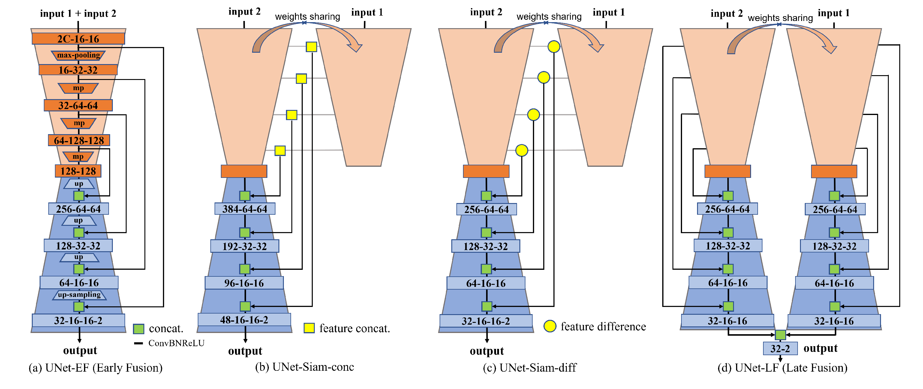
• We evaluated several simple but widely used deep learning architectures for wildfire-burned area mapping, i.e., U-Net and its Siamese variants. We also investigated three fusion strategies, including early fusion, late fusion, and intermediate fusion.

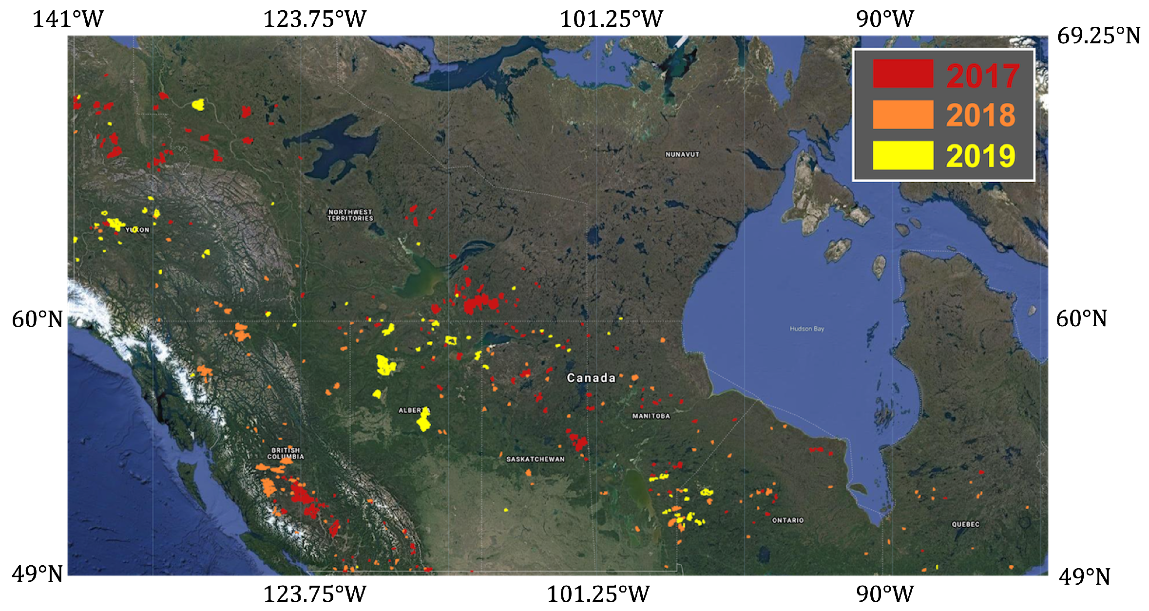
2. Wildfire-S1S2ALOS-Canada Dataset

2.1. Data Sources

The National Burned Area Composite (NBAC) of Canada is a Geographic Information System (GIS) database that has calculated the area of burned forest on a national scale each year since 1986. The NBAC is part of the Fire Monitoring, Accounting, and Reporting System (FireMARS), jointly developed by the Canada Center for Mapping and Earth Observation and the Canadian Forest Service, whose primary data sources are fire polygons derived from 30 m Landsat imagery (using the Multi-Acquisition Fire Mapping System, MAFMS) and high-quality agency polygons delineated from imagery with higher spatial resolution than 30 m. MAFMS polygons achieved an average accuracy of 96% relative to burned area products of high spatial resolution, and the confidence intervals of NBAC is around 4.3% [25].

Considering the data availability of Sentinel-1/2, the 2017–2019 Canadian wildfires were taken as the main study areas/period (see Figure 1). The NBAC products include fire location, fire period, and accurate burned area polygons, which are quite valuable in wildfire monitoring for both remote sensing and the machine learning community. To accelerate the research on deep learning for wildfire monitoring, we created a large-scale optical and SAR satellite imagery dataset of 20 m spatial resolution based on freely available satellite data, such as Sentinel-2 multispectral instrument (MSI) data, Sentinel-1 C-Band SAR data, and ALOS PALSAR/PALSAR-2 L-Band SAR data.

Sentinel-2 MSI Data: Sentinel-2 is a high-resolution (10 m) multispectral imaging mission that supports Copernicus Land Monitoring studies, which consists of a constellation of two polar-orbiting satellites placed in the same sun-synchronous orbit, phased at ${180}^{\circ }$ to each other. The Sentinel-2 mission has global coverage and high revisit time, 10 days at the equator with one single satellite, and 5 days with 2 satellites, which plays an important role in monitoring the changes happening on the Earth’s surface. A detailed description can be found in the Harmonized Sentinel-2 Level-1C Top-of-Atmosphere (TOA) products [26]. All Sentinel-2 scenes were clipped into the range [0, 5000] and then normalized into the range [0, 1] by dividing 5000.

Sentinel-1 C-Band SAR Data: The Sentinel-1 mission includes two C-Band SAR satellites, i.e., Sentinel-1A and Sentinel-1B, which provide high-resolution dual-polarization SAR data acquired with a wavelength of 5.6 cm. Sentinel-1 Ground Range Detected (GRD) scenes are available in GEE, where each scene has been preprocessed to derive the backscatter coefficient with the Sentinel-1 Toolbox using the following steps: (1) thermal noise removal; (2) radiometric calibration; (3) terrain correction; (4) log scaling into decibels via 10${log}_{10}\left(x\right)$. For Sentinel-1 SAR data, we calculated the Normalized Difference Backscatter Index (NDBI, shorted as ND) via $\mathrm{ND}=\frac{\mathrm{VV}-\mathrm{VH}}{\mathrm{VV}+\mathrm{VH}}$, where VH and VV are in power units, and the ND band was converted into dB via $10{log}_{10}\left(x\right)$.

ALOS-2 PALSAR-2 L-Band SAR Data: Both ALOS/PALSAR and ALOS-2/PALSAR-2 are L-Band SAR sensors launched in 2006 and 2014, respectively (with 14 days revisit time), which image at a wavelength of 24 cm. ALOS PALSAR was in operation from 2006 to 2011, while ALOS-2 PALSAR-2 has been in operation since 2014. ALOS-4 PALSAR-3 was planned to launch in 2023. L-band microwaves can reach the ground by partially penetrating through vegetation to obtain information on vegetation structure and the ground surface. Compared to ALOS PALSAR, the ALOS-2 PALSAR-2 became a unique and highly useful sensor achieving high resolution, wide swath width, and good image quality, which allows for comprehensive monitoring of disasters. Available in GEE, the global 25 m ALOS PALSAR/PALSAR-2 Yearly Mosaic product is a seamless global SAR image created by mosaicking strips of SAR imagery selected through visual inspection over each year and showing minimum response to surface moisture. For convenience, ALOS-2 PALSAR-2 L-Band SAR is shortened to ALOS here and after. For ALOS L-Band SAR data, the HH and HV polarizations were stored in Digital Number (DN), and the ND band was calculated using $\mathrm{ND}=\frac{\mathrm{HH}-\mathrm{HV}}{\mathrm{HH}+\mathrm{HV}}$. Then, HH, HV, and ND bands in power units were converted to gamma naught values in decibel unit (dB) using log-scaling: $10{log}_{10}\left(x^2\right)-83$. The ND band was then rescaled by multiplying 3 to match the range of HH and HV in dB.

2.2. Dataset Preparation

Figure 2 shows the workflow of data preparation on the S1S2ALOS-Wildfire dataset based on GEE. The wildfire perimeter database was used to derive the region of interest (ROI), fire year y, and fire period [$t_{start},t_{end}$], where $t_{start}$ and $t_{end}$ denote the time when a fire started and ended. First, we filtered the Sentinel-2 image collection with the ROI filter and the cloud filter with a cloud percentage lower than 20%. We applied the date filter [$t_{start}$− 1 year, $t_{end}$− 1 year] to obtain the pre-fire time series, masked the cloudy areas, and calculated its median as the pre-fire image. Similarly, we applied the date filter [$t_{end}$, $t_{end}$ + 2 month] to obtain the post-fire time series, masked the cloudy areas, and calculated its median as the post-fire image. If the generated images are not in good quality visually, the post-fire period will be replaced by the images acquired in [$t_{start}$ + 1 year, $t_{end}$ + 1 year]. For Sentinel-1, we first calculated all available relative orbits and then conducted orbit-wise data preprocessing. For each orbit, we filtered pre-fire and post-fire time series with date filter [$t_{start}$ − 1 year, $t_{end}$ − 1 year] and [$t_{end}$, $t_{end}$ + 2 month], respectively, and then calculated the corresponding average images as the pre-fire and post-fire images. For ALOS-2 PALSAR-2, since only global yearly mosaic products are available in GEE, we took the year (y− 1) as the pre-event image and the year (y + 1) as the post-event image for an event that happened in the year y. Additionally, the wildfire perimeters were rasterized as the ground reference mask.

After the preparation of multi-source pre-fire and post-fire images for every wildfire event, we exported them into Google Cloud Bucket together with rasterized reference masks at a spatial resolution of 20 m in the format of Cloud-Optimized GeoTiff (COG). For each wildfire event, we exported both Sentinel-1 VH and VV polarized images acquired on different orbits and the corresponding ND band, and we exported 6 bands for Sentinel-2, including Red, Green, Blue, Near-Infrared (NIR), Short-Wave Infrared 1-/2 (SWIR-1 and SWIR-2)—the most sensitive bands.

By downloading the exported data from Google Cloud Storage to a local machine, a visual inspection was conducted to exclude samples in poor quality. Each group of S1 pre-post, S2 pre-post images, AL pre-post images, and the corresponding reference masks was converted to a visually perceivable format, as shown in Figure 2. If either of these four images contains very large no-data areas, large clouds, or mosaicing-caused artifacts, that group of images would be discarded. The remaining images were mirror padded into an integer time of 256, both in height and width, and then tiled into patches of the shape 256 × 256 in a stride of 256 pixels; therefore, adjacent patches have no overlap pixels except for the patches containing the pixels generated by mirror padding.

After data cleaning, there are 328 wildfire events left, in which there are 132 events that happened in 2017, 138 events in 2018, and 58 events in 2019. For real-world applications, models should be trained on past events and tested on future events. To simulate this scenario, we used the 2017 and 2018 wildfire events as the training set, and the 2019 wildfire events as the testing set. By tiling all images and the reference masks into the shape of 256 × 256, the final wildfire-burned area dataset contains 9052 groups of training patches (10% taken as the validation set) and 2856 groups of testing patches. Each group of image patches includes Sentinel-2 pre and post-MSI images, Sentinel-1 pre and post-SAR images, ALOS-2 PALSAR-2 pre- and post-SAR images, and the ground reference masks in the format of multi-channel COG. Figure 2 shows a group of images, providing a visual perception of this wildfire-burned area dataset.

2.3. Dataset Structure

This wildfire-burned area dataset was organized in a tree-like structure with two main branches, i.e., train and test. In both the train and test folder, there are four subfolders, such as S1, S2, ALOS, and mask, which denote Sentinel-1, Sentinel-2, ALOS-2 PALSAR-2, and the reference mask, respectively. Each of them contains two subfolders named ‘pre’ and ‘post’ that include pre-fire and post-fire image patches. The individual events can be identified by the filename of COG, i.e., event_id, and the tiled image patches were named by the following scheme event_id_row_col.tif, where row and col represent the location of this patch in the 256 × 256 grid of the original imagery before tiling.

3. Optical and Radar Responses to Burned Areas

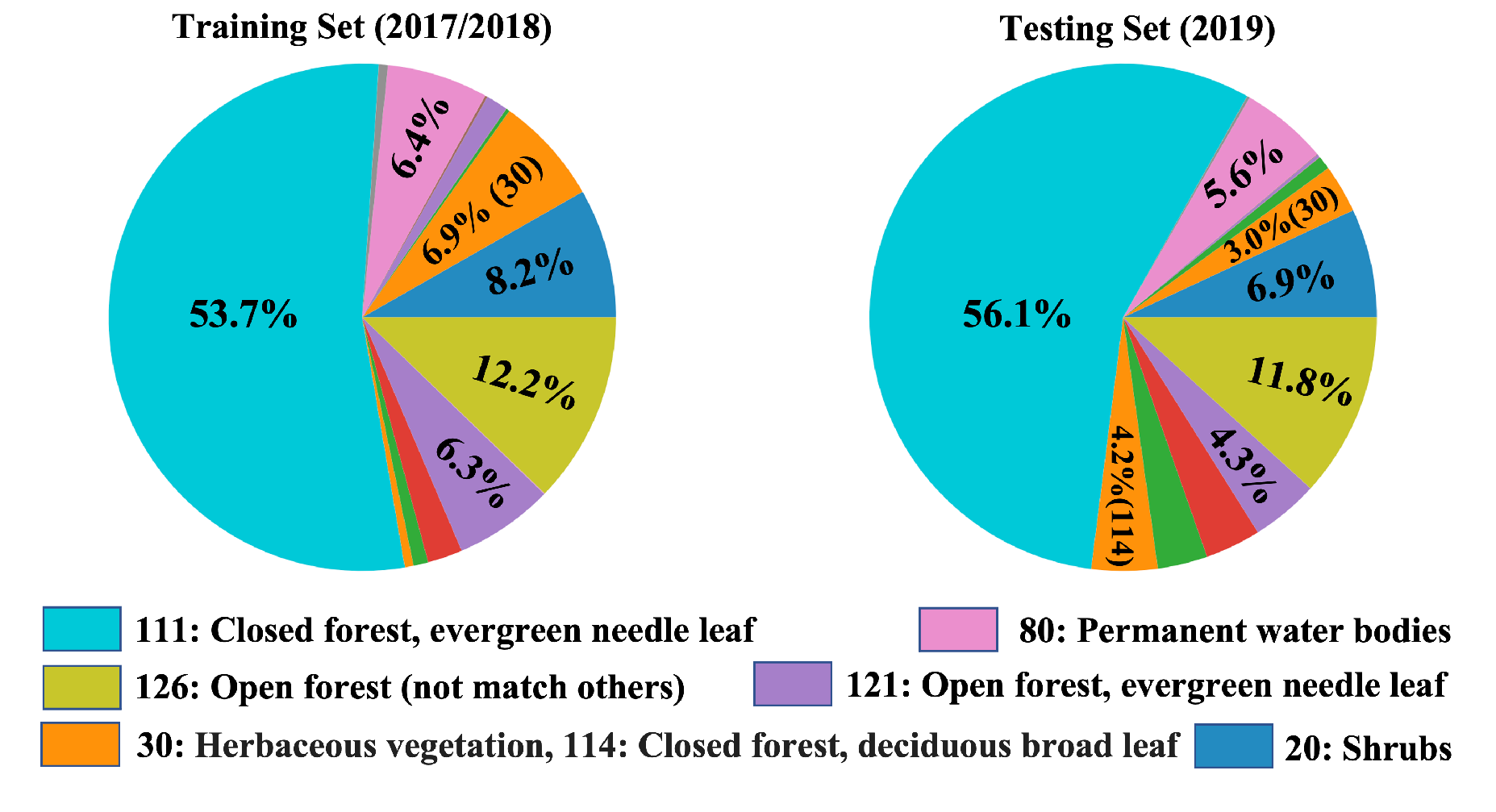
3.1. Land Cover Distribution

Figure 3 shows the land cover distribution of the proposed data in training and testing sets. The dominant land cover type is the closed forest with evergreen needle leaf in both training and testing sets, while open forest (class values: 121, 126) occupies about 18.5% in the training set and 16.1% in the testing set. In total, 8.2% of land cover is shrubs in the training set and 6.9% in the testing set, and the remaining main land cover includes permanent water bodies, herbaceous vegetation, and closed forest with deciduous broad leaf.

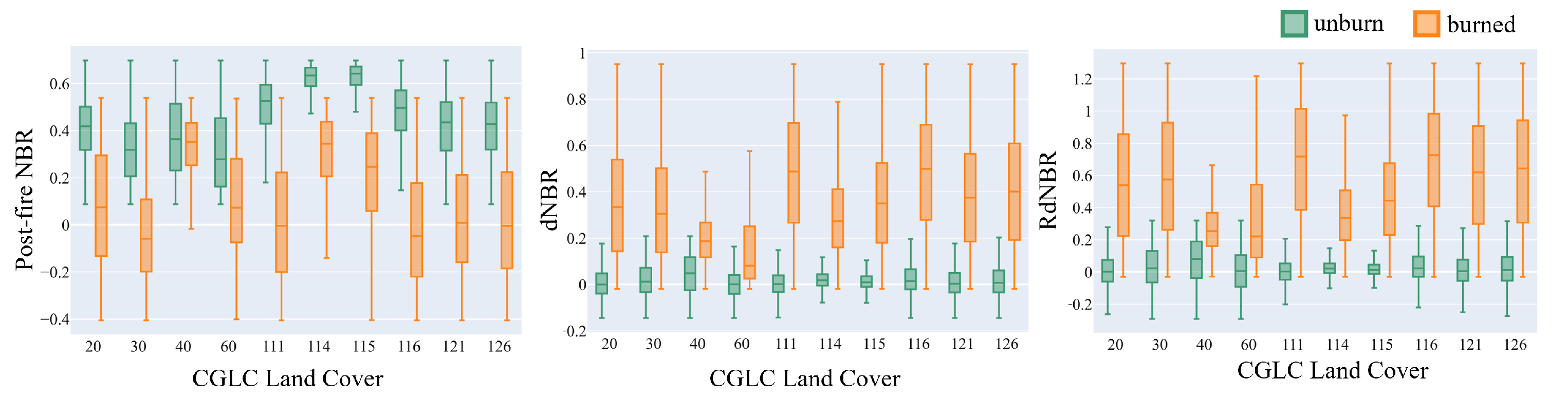
3.2. Sentinel-2 Spectral Responses

Figure 4 shows the difference between healthy and burned vegetation in post-fire NBR, dNBR, and RdNBR with respect to land cover types, where $\mathrm{NBR}=\frac{\mathrm{NIR}-\mathrm{SWIR}}{\mathrm{NIR}+\mathrm{SWIR}}$, $\mathrm{dNBR}={\mathrm{NBR}}_{pre}-{\mathrm{NBR}}_{post}$, and $\mathrm{RdNBR}=\frac{\mathrm{dNBR}}{\sqrt{{\mathrm{NBR}}_{pre}}}$. It is worth noting that both the unburned and burned pixels were randomly sampled based on the reference mask. (1) For different land cover types, the burned vegetation has significantly wider spreads and longer boxes than healthy vegetation in the post-fire NBR, dNBR, and RdNBR; (2) the dNBR median value of healthy vegetation is close to 0, while that of burned vegetation is higher than 0.3 expect for the agriculture (CGLC: 40) and sparse vegetation areas (CGLC: 60); (3) most of land cover types follow a normal distribution in dNBR and RdNBR before and after wildfire burning, and there is no significant difference in the distribution of dNBR and RdNBR. (4) The closed forests (including deciduous broad leaf and mixed, CGLC: 114 and 115) show a higher post-fire NBR than other land cover in unburned areas.

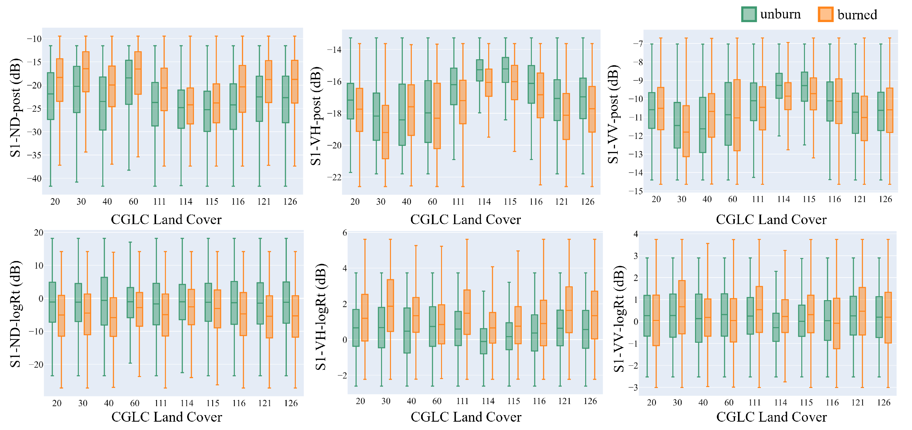
3.3. Sentinel-1 C-Band SAR Backscatter Responses

Figure 5 shows the comparison among post-fire and log-ratio differenced Sentinel-1 ND (Normalized Difference Backscatter Index, NDBI), VH, and VV with respect to land cover types. From the post-fire backscatter charts, we observed that: (1) the post-fire SAR backscatter seems to follow a normal distribution, and there is a relatively high overlapping between unburned and burned areas for various land covers. (2) CGLC-114 and CGLC-115 have a smaller box and shorter spreads than other land covers in post-fire VH and VV SAR backscatter, with the highest median values. (3) For most land covers, burned vegetation has a lower VH and VV backscatter than healthy vegetation in the post-fire images but a higher ND value.

From the log-ratio differenced charts, we observed that: (1) the log-ratio differenced ND follows a normal distribution with a median value close to −1 dB for various land covers in unburned areas, while with a median value close to −5 dB in burned areas; (2) the log-ratio differenced VH has a slightly longer box and significantly higher median value (about 1 dB) in burned areas than unburned areas, while the log-ratio differenced VV has a significantly smaller difference between burned and unburned areas compared to VH.

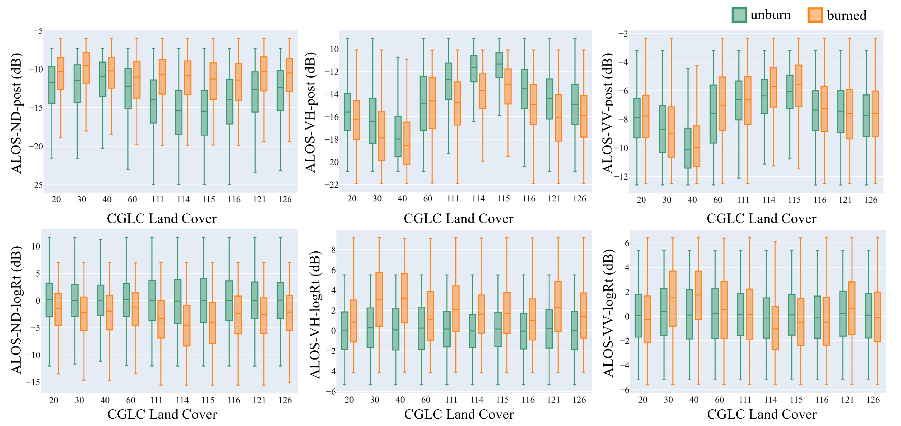
3.4. ALOS-2 PALSAR-2 L-Band SAR Backscatter Responses

Figure 6 shows the comparison among the post-fire ALOS-2 PALSAR-2 L-band backscatter and the log-ratio differenced backscatter between pre-fire and post-fire images with respect to land cover types. From the post-fire backscatter charts, we observed that: (1) in both burned and unburned areas, the post-fire ND, VH, and VV follow a normal distribution with significantly different median backscatter values in various land covers; (2) in unburned areas, healthy vegetation of various land cover types has significantly different backscatter in ND, VH, and VV. Compared to unburned areas, burned areas have a significantly lower VH backscatter but just a slightly different VV backscatter; (3) it is interesting to observe that the post-fire ND backscatter of various land cover tends to follow a very similar distribution in burned areas after being burned, and even the healthy vegetation follows a significantly different distribution in unburned areas.

As shown in the bottom row in Figure 6, from the log-ratio differenced backscatter charts, we observed that (1) in unburned areas, the log-ratio differenced ND, VH, and VV backscatters follow a normal distribution with a median value close to zero; (2) for the log-ratio differenced VH, burned areas have a significantly higher box and median value than unburn areas in various land cover types, while the log-ratio differenced VV shows significant difference in CGLC-30, 40, 114, and 115 between unburn and burned areas; (3) the log-ratio differenced ND also shows a clear difference in distribution between unburned and burned areas.

4. Deep Learning for Wildfire-Burned Area Mapping

As shown in Figure 7, we investigated four classical change detection architectures based on U-Net, including:

• UNet-EF [27]: Fully Convolutional Networks with Early Fusion, where bi-temporal images or multi-source inputs can be stacked along the channel dimension before feeding them into U-Net, and the detailed architecture is illustrated in Figure 7a;
• Siam-UNet-Conc [27]: Siamese U-Net with intermediate feature concatenation, in which two encoder branches handle bi-temporal images, respectively, and the concatenated feature representation along the channel is stacked together with the corresponding decoder features of the same width and height (see Figure 7b);
• Siam-UNet-Diff [27]: Siamese U-Net with differenced features from encoders, and the differenced features are stacked together with the corresponding decoder features of the same widths and heights to make the final predictions (see Figure 7c);
• UNet-LF [28]: U-Net with Late Fusion, in which two individual U-Nets handle bi-temporal images independently, and the decoder outputs are stacked or fused together at a very late stage (see Figure 7d).

The above description assumes input-1 and input-2 are bi-temporal images from the same sensor; when it comes to multi-sensor inputs, input1 and input2 can be the satellite images from difference sensors for the architectures shown in Figure 7a,b,d. The Siam-UNet-Diff is not suitable for multi-sensor inputs since the feature difference between different sensors is not meaningful.

Binary Cross-Entropy (BCE) Loss was taken as the default setting for model training, and the learning rate was updated using the cosine annealing scheduler with the starting learning rate of 1 $\times {10}^{-4}$ and 10 warm-up steps. All models were trained within 100 epochs with a batch size of 16 and a weight decay of 0.01 without any data augmentation and dropout. Figure 7 shows the used network architectures, all of which were implemented with PyTorch and all experiments were run on a single NVIDIA GTX3080 GPU with 10GiB RAM. The weight-sharing can be enabled for single-sensor bi-temporal inputs, but our experiments show enabling weight-sharing between branches did not bring about significant improvement. Therefore, all experiments shown in this work were obtained without enabling weight-sharing.

Table 1. Input data settings.

Satellite	Setting Name	Bands	Pre-Fire	Post-Fire
Sentinel-2 (S2)	post	B4, B8, B12		√
	prepost	B4, B8, B12	√	√
Sentinel-1 (S1)	VV	VV	√	√
	VH	VH	√	√
	ND	ND	√	√
	post	ND, VH, VV		√
	prepost	ND, VH, VV	√	√
ALOS-2 PALSAR-2 (AL)	HH	HH	√	√
	HV	HV	√	√
	ND	ND	√	√
	post	ND, HV, HH		√
	prepost	ND, HV, HH	√	√

shows the abbreviated names of various input settings. For instance, the “post” denotes that the model only takes post-fire image bands as input, while “prepost” indicates that the model takes both pre-fire and post-fire images as input. For S1 and ALOS SAR data, “VV”, “VH“, and ”ND“ denote the model taking both pre-fire and post-fire VV, VH, and ND bands, respectively, in this section. In Figure 4, Figure 5 and Figure 6, the comparison of the optical and radar response to burned areas demonstrates the capability of optical data in highlighting burned areas and the limitation of radar data in the data space. Spectral indices (e.g., NBR and dNBR) were not fed into U-Net since neural networks have the capability to learn the desired features from the original spectral bands: B4, B8, and B12.

5. Experimental Results

Figure 8 compares two approaches for calculating the IoU score on the testing set, i.e., the average IoU score and the total IoU score. Different wildfire events may have various sizes of burned areas, leading to different shapes of data. As mentioned above, we tiled different shapes of remote sensing data and the corresponding reference masks into patches of the same shape—256 × 256. When the data shape is not a multiple of 256, we expanded the original data by mirroring along the right or bottom border pixels, which would introduce repeated pixels in the tiled version. The average IoU score means that we first calculated the patch-wise IoU and then averaged all the IoU scores, while the total IoU score was calculated by accumulated TP, FP, and FN pixels over all testing fires without any repeated pixels. Hereafter, we report the average IoU by default.

From Figure 8, we observed that the total IoU score has a higher value than the average IoU score. (1) For S2, the total IoU score is slightly higher than the average IoU in the prepost setting, while a 0.05 increase was observed in the post setting. (2) For S1, the most significant difference (0.2 in IoU) was observed in the post setting, and we also observed that the total IoU score brought about a 0.05 to 0.08 increase compared to the average IoU score in other settings. (3) For ALOS, the least IoU difference (0.03 in IoU) was observed in the post setting, and the difference between the total IoU and the average IoU fell between 0.05 to 0.1 for the other settings.

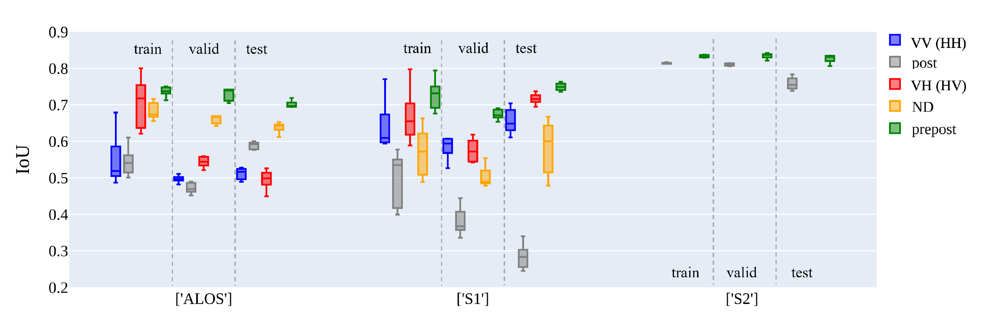
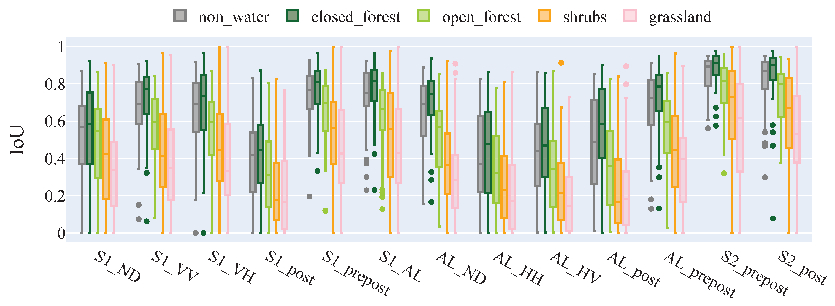
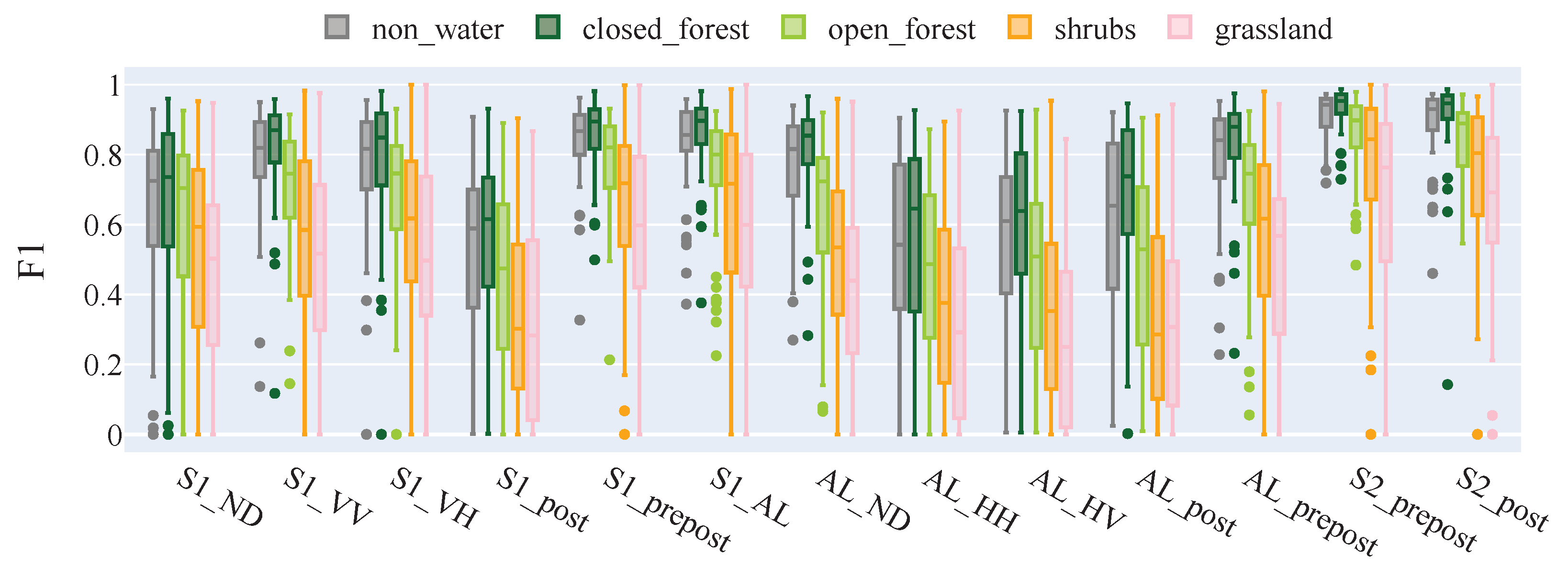
5.1. Channel Evaluation with U-Net

Figure 9 shows the performance comparison of U-Net on S1, ALOS, and S2 data with various input channels. It is observed that (1) for S2, the prepost setting achieved a slightly higher IoU score than post image alone, and different runs have a relatively low IoU variance in both training and validation sets. Compared to the validation set, the post setting shows a 0.05 decrease in IoU score on the testing set while prepost shows almost no decreases in IoU with a slightly larger variance. (2) For S1, the prepost setting achieved the highest IoU score while the post setting obtained the lowest IoU score across the training, validation, and testing sets. Bi-temporal stacked VH achieved the highest IoU score, followed by VV and ND. Except for the post setting, all other settings achieved higher IoU scores in the testing set than the validation set, which may imply that the model trained only with post-fire images has poor generalization performance. (3) For ALOS, the prepost setting achieved the highest IoU score across the training, validation, and testing set, followed by the ND setting. The VH setting achieved significantly higher IoU than the VV setting in both training and validation sets but not in the testing set. The post setting achieved a 0.1 higher IoU score in the testing set than the validation set, which is quite different from the observations on the S1 data. (4) Except for the VH and VV setting, ALOS-based results have a smaller box than S1-based ones. For both ALOS and S1, the prepost setting achieved the highest IoU score. For ALOS, the performance ranking is prepost > ND > HV > post > HH, while for S1, the performance ranking is prepost > VH > VV > ND > post.

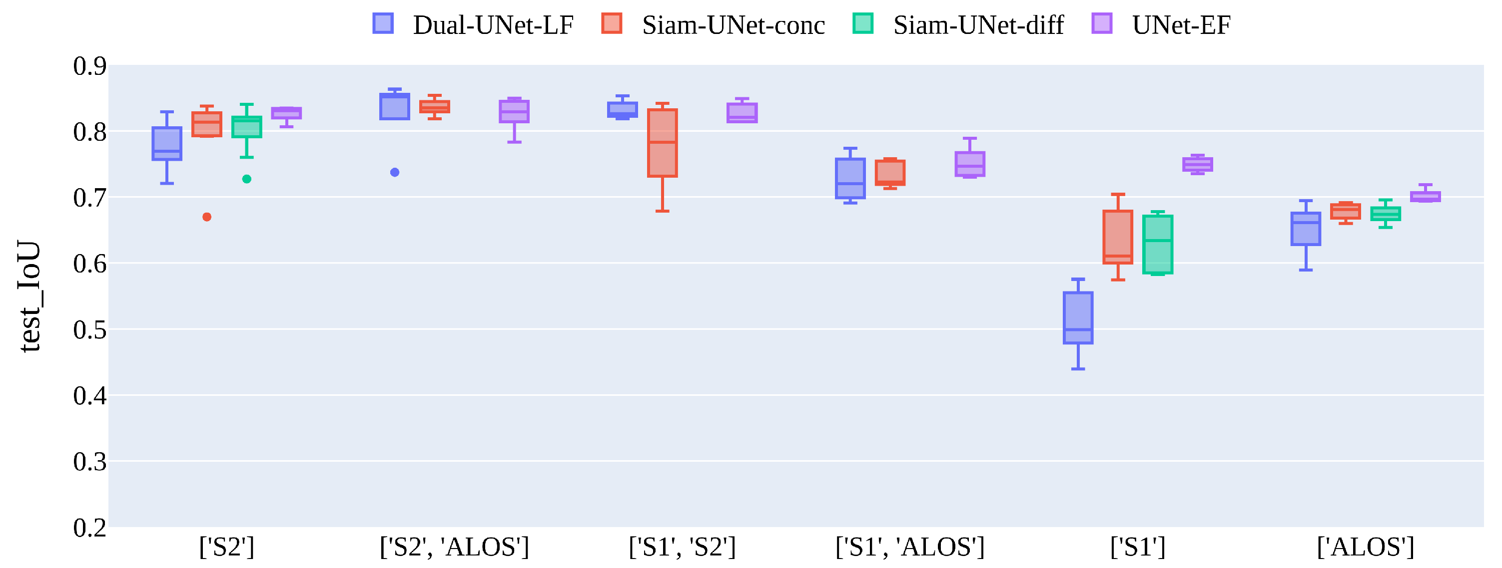
5.2. Single-Sensor vs. Multi-Sensor Fusion

Figure 10 shows the quantitative comparison among four classical change detection architectures based on bi-temporal data acquired by a single sensor or any two sensors from Sentinel-2, Sentinel-1 and ALOS-2 PALSAR-2. (1) For a single sensor, whether it is S2, S1, or ALOS, U-Net achieved the highest IoU score with the smallest box, followed by the two Siamese U-Net, and the DuelUnet_LF obtained the lowest IoU score with a relatively larger box. For S2 and ALOS, U-Net achieved slightly higher accuracy than these two Siamese U-Net with concatenated or differenced features, which also performed slightly better than the DuelUnet_LF. But for S1, we observed that U-Net achieved a 0.1 higher IoU than these two Siamese U-Nets and 0.25 higher IoU than the DuelUnet_LF. No significant difference was observed between SiamUnet_conc and SiamUnet_diff on the proposed wildfire dataset. (2) For the multi-sensor fusion settings, we fed different sources of data into two branch subnetworks of SiamUnet_conc and DualUnet_LF. There is no SiamUnet_diff anymore because it is not meaningful to differentiate the features from different sensors. We investigated the fusion performance by fusing any two of these three sensors, i.e., S2, S1, and ALOS. For the S2-ALOS fusion and the S1-S2 fusion, all three architectures achieved almost the same accuracy except for the exceptional SiamUnet_conc in the S1-S2 fusion. For the S1-ALOS fusion, UNet performed slightly better than the other two. (3) From the cross-comparison among single- and multi-sensors, we observed that the S2-ALOS fusion and S1-S2 fusion performed slightly better than S2 itself and achieved significantly higher IoU than S1 or ALOS. The S1-ALOS multi-frequency fusion performed significantly better than S1 and ALOS, and U-Net achieved the highest accuracy in SAR-based results.

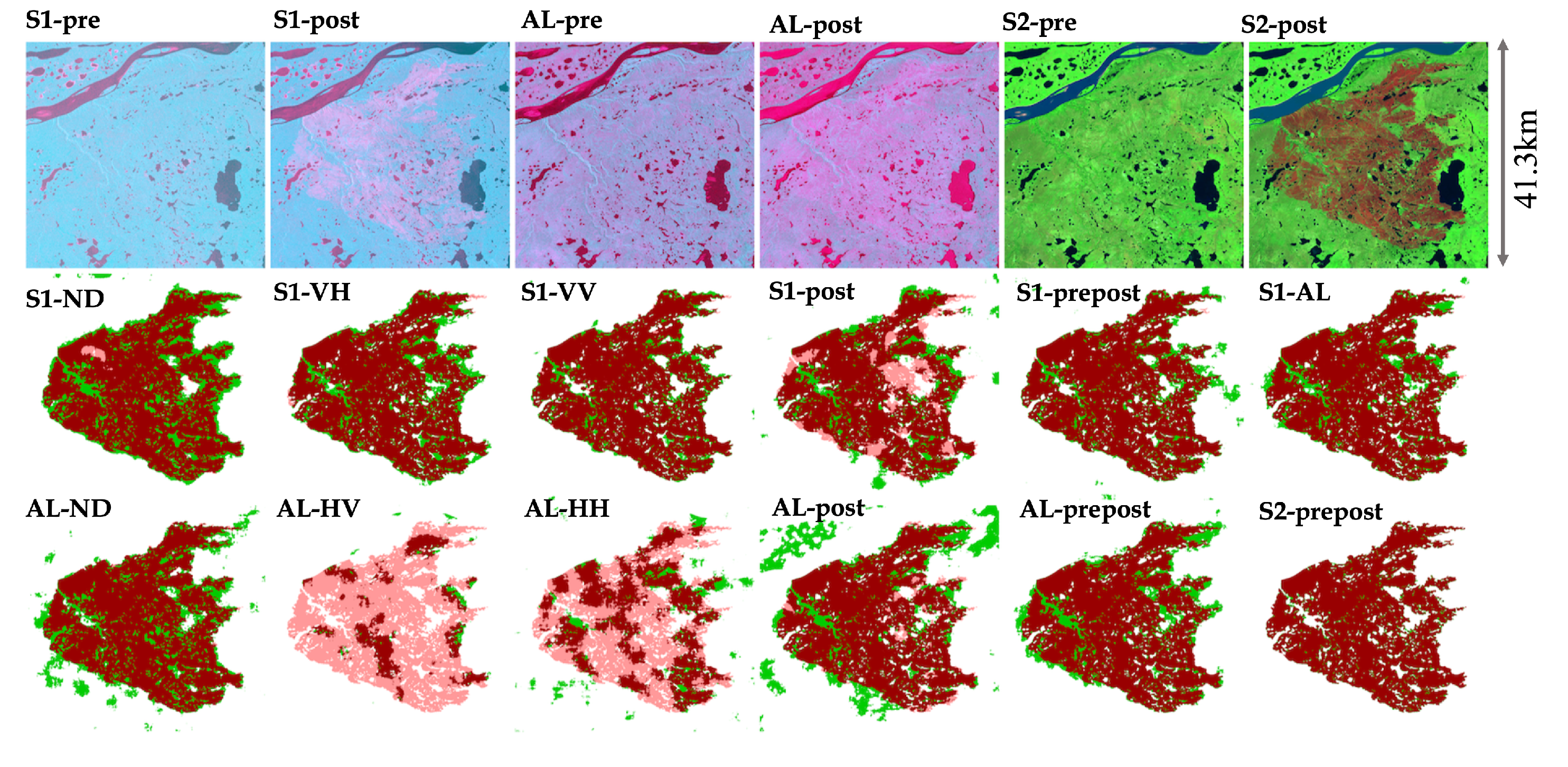
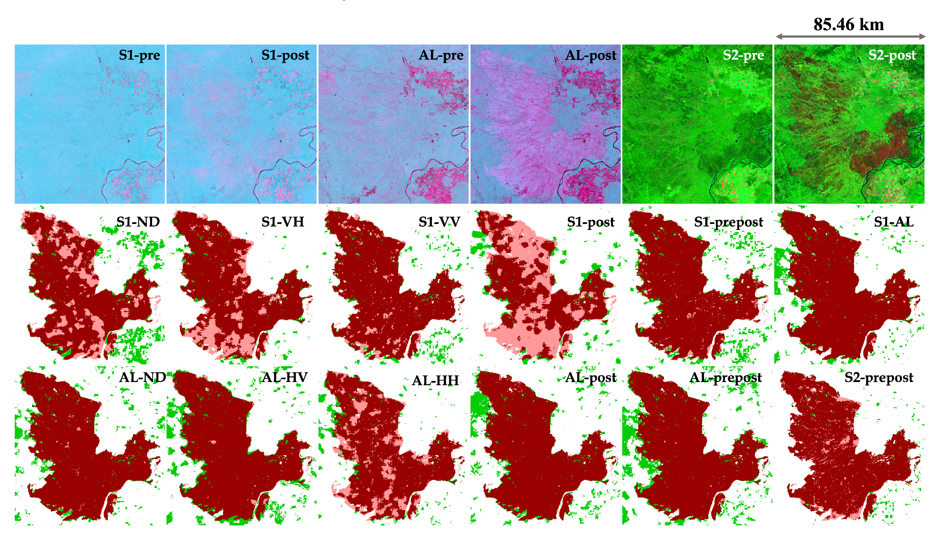
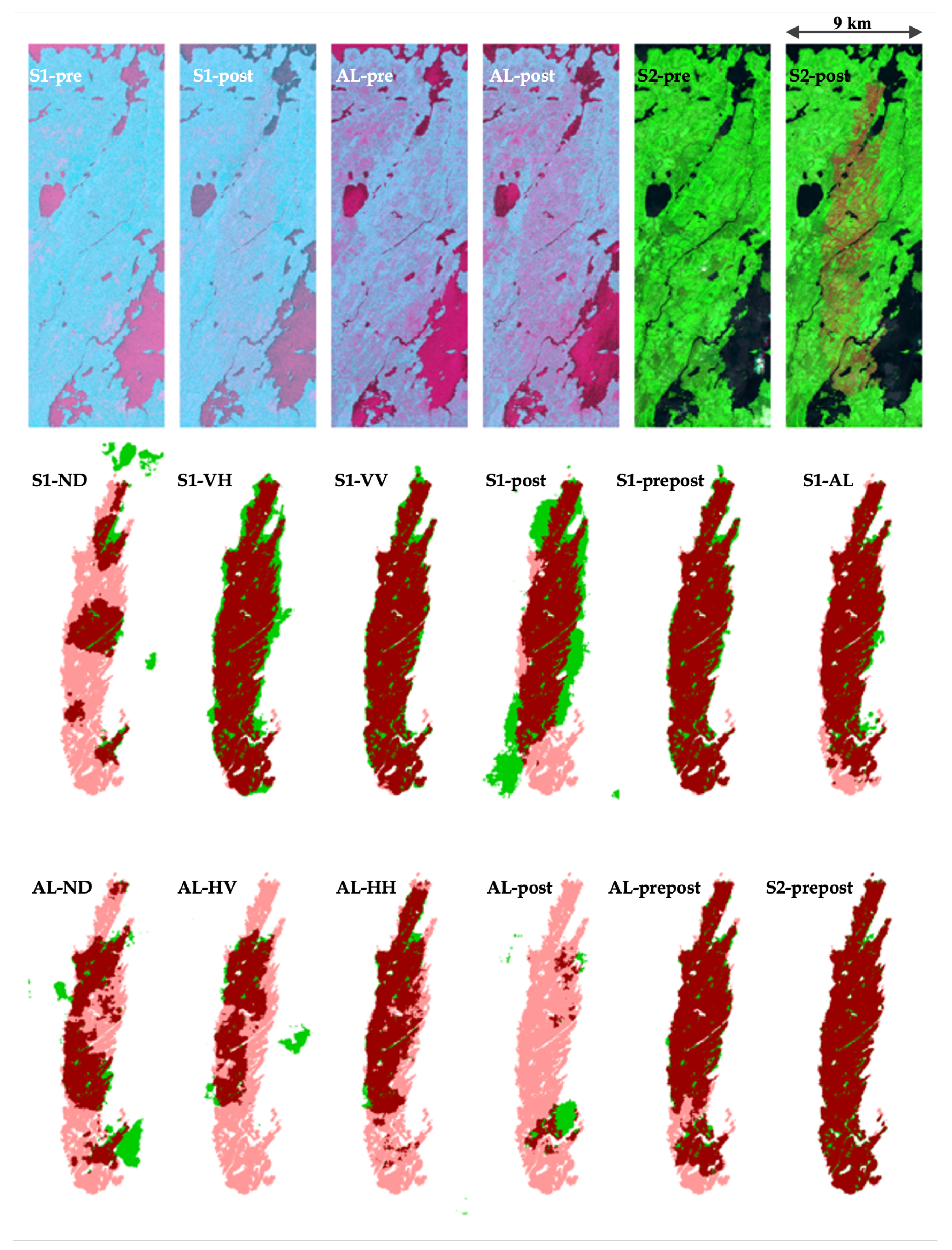
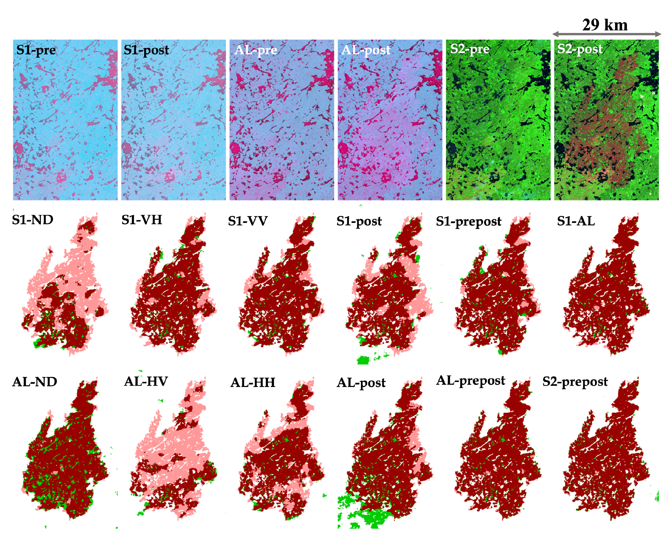
5.3. Visual Comparison

Figure 11, Figure 12, Figure 13 and Figure 14 show the visual comparison among 12 different settings on four wildfire events, i.e., CA-2019-NT-8, CA-2019-AB-172, CA-2019-QC-808, and CA-2019-ON-730. From Figure 11, we observed that (1) both Sentinel-2 and Sentinel-1 post-event images show the burned area quite clearly, and ALOS PALSAR post images also show the detectability of the burned area, but its visibility is not as good as the other two; (2) all pre-event images from these three sensors look good visually and show decent consistency in unburned areas between pre- and post-event images; (3) Sentinel-2 achieved the best visual results on the CA-2019-NT-8 wildfire, and AL-VH and AL-VV are the worst two. As for the CA-2019-AB-172 fire in Figure 12, we observed that (1) the ALOS PALSAR post-event image shows the best visibility of burned areas, while the burned area connectivity looks low visually in both Sentinel-2 and Sentinel-1 post-event images; (2) Sentinel-2 achieved the best visual results, and most results detected the burned areas correctly, while S1-post and S1-ND are among the worst ones. As shown in Figure 13, we observed S1-prepost, S1+ALOS, ALOS-prepost, and S1-VH achieved decent results on the CA-2019-QC-808 fire event, while S1-ND, S1-post, AL-ND, and AL-post are among the worst. On the CA-2019-ON-730 fire, we found most results show good consistency with the ground truth, but S1-ND and AL-VH are quite bad. Both S1-post and ALOS-post show a few FP pixels in the bottom left corner, and the FP pixels disappeared when the pre-event image was used.

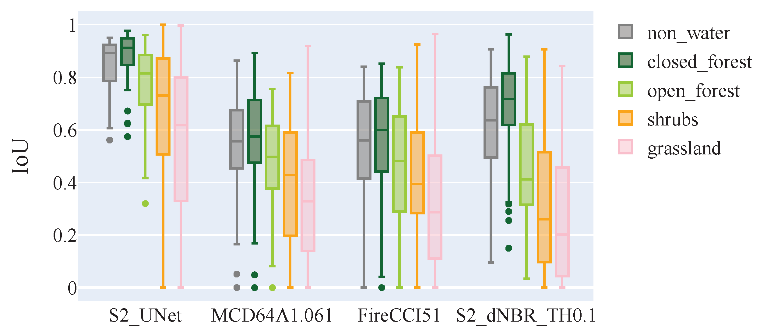
5.4. Land Cover-Specific Assessment

Figure 15 and Figure 16 present the IoU (Intersection over Union) and F1 score boxplots for U-Net models, tested on 58 events across land cover types such as closed forests, open forests, shrubs, and grasslands. Recognizing that wildfires affect only non-aquatic regions, we refined our model assessment by exclusively considering non-water pixels, excluding aquatic zones on an event-specific basis. From the IoU and F1 boxplots, we observed that: (1) S2_prepost achieved the best performance among all settings and across various land cover types, and the closed forest shows the narrowest spreads, followed by open forest, shrubs, and grassland. (2) U-Net predominantly attained the highest IoU and F1 scores in closed forests, followed by non-water areas, open forests, shrublands, and grasslands, with exceptions noted for AL_ND and S2_post cases. (3) The S1_post showed a remarkable decline in accuracy without pre-event imagery compared to the S1_prepost. S1_prepost obtained higher accuracy than AL_prepost, while the S1_post achieved a lower accuracy than AL_post when the pre-event image was removed. Additionally, the prepost settings generally have narrower spreads than the post settings. (4) In non-water areas, S1_VH achieved a similar accuracy to S1_VV but a wilder spread, whereas AL_VH showed higher accuracy than AL_VV. S1_ND showed lower accuracy compared to S1_VH and S1_VV, while AL_ND showed a significantly higher accuracy than AL_VH and AL_VV, with narrower IQR spreads, especially in non-water and closed forest areas. (5) S1_AL achieved an accuracy close to S1_prepost and AL_prepost with slightly narrower spreads in non-water and forest areas. (6) Without pre-event information, S2_post obtained a slightly lower median accuracy than S2_prepost in all vegetation types.

5.5. Comparison between Sentinel-2 and MODIS-Based Burned Area Products

Figure 17 shows the comparison between Sentinel-2 and MODIS-based burned area products across various vegetation types. In this figure, S2_UNet denotes the UNet prediction based on Sentinel-1 pre-fire and post-fire images, S2_dNBR_TH0.1 denotes the detection based on thresholding S2_dNBR with the specified threshold 0.1, while MCD64A1.061 and FireCCI51 are two global burned area products based on MODIS. MCD64A1.061 is a monthly global 500 m burned area product, which was generated by using burn sensitive vegetation index to create dynamic thresholding. FireCCI51 is a monthly global 250 m spatial resolution product that was generated using a two-phase hybrid approach: (1) detecting pixel seeds with a high probability of being burned based on active fires; (2) adaptive thresholding-based seed growing.

From both Figure 17 and

Table 2. Quantitative Comparison Between Sentinel-2 and MODIS-Based Burned Area Products over 58 Testing Events (the median IoU or F1 scores are reported in this table).

	Product	Non_Water	Closed_Forest	Open_Forest	Shrubs	Grassland	Others
IoU	S2_UNet	0.89	0.91	0.82	0.73	0.62	0.67
	MCD64A1.061	0.56	0.58	0.50	0.43	0.33	0.40
	FireCCI51	0.56	0.60	0.48	0.39	0.29	0.38
	S2_dNBR_TH0.1	0.64	0.72	0.41	0.26	0.20	0.25
F1	S2_UNet	0.94	0.95	0.90	0.84	0.76	0.80
	MCD64A1.061	0.71	0.73	0.66	0.60	0.49	0.57
	FireCCI51	0.72	0.75	0.65	0.56	0.45	0.55
	S2_dNBR_TH0.1	0.78	0.84	0.58	0.41	0.34	0.40

, we observed that S2_UNet achieved the highest IoU and F1 scores over various vegetation types, and the accuracy is significantly higher than the rest of the products. S2_dNBR thresholding achieved slightly higher IoU and F1 scores than MODIS-based two products, i.e., MCD64A1.061 and FireCCI51 over non-water pixels and closed forest, but showed lower accuracy in open forest, shrubs, and grassland. MCD64A1.061 and FireCCI51 show similar accuracy over different vegetation types, with an overall IoU of 0.56 and F1 of 0.71–0.72 in the non-water areas. MCD64A1.061 achieved slightly lower accuracy than FireCCI51 in closed forest, but higher accuracy in open forest, shrubs, grassland, and others.

6. Discussion

This research does not endeavor to introduce a novel model or architecture; rather, it seeks to offer valuable perspectives on the effectiveness of SAR across a range of land cover types. We accomplish this through a thorough comparative analysis of multi-source and multi-frequency SAR data applied to large-scale mapping of wildfire-affected areas. Drawing upon the 2017–2019 Canadian wildfires, we have constructed a comprehensive benchmark dataset for large-scale wildfire-burned area mapping. This dataset facilitates a meticulous examination of data distributions, the performance of various network architectures, and an accuracy assessment tailored to specific land cover types.

Figure 4 suggests that Sentinel-2 post-event Normalized Burn Ratio (NBR) effectively discriminates between burned and unburned samples across most land cover types, with the notable exceptions of agricultural and sparse vegetation areas, where we observe an overlap within the IQR. By contrasting post-event NBR with pre-event values (dNBR), we notice a convergence towards zero in unburned zones, markedly enhancing separability in agricultural and sparse vegetation areas. Thus, a judiciously chosen threshold on Sentinel-2 data could yield satisfactory results. However, this approach does not extend to SAR data. Figure 5 and Figure 6 demonstrate a pronounced overlap in IQR between burned and unburned boxplots, regardless of whether examining post-event backscatter or log-ratio backscatter changes, making it challenging to set a definitive threshold for burn detection. Log-ratio backscatter alterations indicate marginally better separation potential. Notably, ALOS-2 PALSAR-2’s ND band exhibits remarkable performance in closed forest settings. These findings are primarily derived from boreal wildfire events, and additional data from other climatic regions is necessary to reinforce these insights.

Our analysis of four classical network architectures for change detection in remote sensing, applied to our wildfire dataset, is summarized in Figure 10. The comparative results from three individual sensors (Sentinel-2, Sentinel-1, and ALOS-2 PALSAR-2) show that U-Net outperforms others with the highest IoU scores and the narrowest IQR. When it comes to combining Sentinel-2 with SAR data, UNet-LF marginally surpasses SiamUNet_conc and U-Net in IoU scores. U-Net prevails in integrating Sentinel-1 C-Band with ALOS PALSAR L-Band data. This study anticipated that the fusion of optical and SAR data might not substantially enhance accuracy in detecting burned areas due to the inherent proficiency of optical data under clear conditions. Nonetheless, there is room for refinement in both learning algorithms and fusion methodologies to more effectively leverage the complementary nature of multi-source data.

The IoU and F1 boxplots in Figure 15 and Figure 16 indicate Sentinel-1 C-Band SAR has better potential in detecting burned areas than ALOS-2 PALSAR-2 L-Band SAR across various land cover types, but Sentinel-1 depends more on pre-fire information than ALOS-2 PALSAR. Compared to C-Band and L-Band SAR, optical data, like Sentinel-2 and Landsat, still attain the best performance when cloud-free images are available. For SAR data, the combined use of multi-polarization bands can achieve higher accuracy than single polarization, and the normalized difference between L-Band HH and HV shows better potential than HH or HV polarization. The results over all settings consistently show both optical and radar data perform best in closed forests, followed by open forests, shrubs, and grassland. In Table 2, the quantitative comparison between Sentinel-2 and MODIS-based burned area products demonstrates the potential of modern medium-resolution satellite data in large-scale burned area mapping (S2: 0.89, MODIS: 0.56 in terms of IoU), and the use of a deep learning approach can significantly improve wildfire detection accuracy compared to a traditional dNBR thresholding approach (an increase in IoU from 0.64 to 0.89).

The research also acknowledges certain limitations. It is worth noting that the L-band data are based on the annual ALOS-2 PALSAR-2 mosaic in GEE over Canada, while annual data can capture the temporal backscattering changes in burned areas where slower or no recovery was observed but may not capture it in regions where fast post-fire recovery is observed. Figure 3 highlights the presence of class imbalance relative to land cover types within the dataset, which could induce model bias. This could potentially be mitigated through the implementation of stratified sampling and the adoption of class-aware weighting within the modeling approach. Moreover, to improve the robustness and applicability of the findings, there is a need to broaden the dataset on a global scale, incorporating more diverse vegetation types and climate zones.

7. Conclusions

In this paper, we presented a large-scale multi-source and multi-frequency satellite image change detection dataset for wildfire-burned area mapping based on Sentinel-2 MSI, Sentinel-1 C-Band SAR, and ALOS-2 PALSAR-2 L-Band SAR data, with the reference masks derived from Landsat data. We conducted a systematic evaluation of the capability of multi-source satellite data in detecting burned areas by comparing the distribution of burned and unburned areas across various land cover types. Generally, bi-temporal differences (such as optical dNBR or SAR-based log-ratio) show superior separability than solely post-event observation. While post-event Sentinel-2 imagery displayed considerable capability, bi-temporal inputs consistently delivered the highest IoU scores. Our analysis, underpinned by the U-Net architecture, revealed that C-Band SAR’s effectiveness is significantly enhanced by incorporating pre-event data, a necessity less pronounced for L-Band SAR. In polarization assessments, C-Band’s VH polarization emerged as most effective, whereas L-Band’s highest IoU was attained with the normalized difference between HH and HV polarizations. Focusing on single-sensor inputs, U-Net recorded the most accurate results. However, the late fusion approach demonstrated a slight edge in integrating optical and SAR data. A land cover-specific accuracy assessment of 58 test wildfires revealed a trend: all sensor configurations attained peak accuracy within closed forests, with a sequential decrease in open forests, shrublands, and grasslands. Notably, L-band’s normalized difference presented higher accuracy than VH and VV. Our study’s scope, concentrated on the 2017–2019 Canada wildfires, primarily in boreal regions, underscores the necessity for a broader spatial and temporal dataset expansion. This will be crucial to refining our understanding of the potential of multi-source satellite remote sensing in large-scale wildfire-burned area mapping.

References

1. Lizundia-Loiola, J.; Otón, G.; Ramo, R.; Chuvieco, E. A spatio-temporal active-fire clustering approach for global burned area mapping at 250 m from MODIS data. Remote Sens. Environ. 2020, 236, 111493. [Google Scholar] [CrossRef]
2. Shi, K.; Touge, Y. Characterization of global wildfire burned area spatiotemporal patterns and underlying climatic causes. Sci. Rep. 2022, 12, 644. [Google Scholar] [CrossRef] [PubMed]
3. Loehman, R.A.; Reinhardt, E.; Riley, K.L. Wildland Fire Emissions, Carbon, and Climate: Seeing the Forest and the Trees—A Cross-Scale Assessment of Wildfire and Carbon Dynamics in Fire-prone, Forested Ecosystems. For. Ecol. Manag. 2014, 317, 9–19. [Google Scholar] [CrossRef]
4. Lasslop, G.; Coppola, A.I.; Voulgarakis, A.; Yue, C.; Veraverbeke, S. Influence of Fire on the Carbon Cycle and Climate. Curr. Clim. Chang. Rep. 2019, 5, 112–123. [Google Scholar] [CrossRef]
5. Palm, E.C.; Suitor, M.J.; Joly, K.; Herriges, J.D.; Kelly, A.P.; Hervieux, D.; Russell, K.L.; Bentzen, T.W.; Larter, N.C.; Hebblewhite, M. Increasing Fire Frequency and Severity will Increase Habitat Loss for a Boreal Forest Indicator Species. Ecol. Appl. 2022, 32, e2549. [Google Scholar] [CrossRef] [PubMed]
6. Hu, X.; Zhang, P.; Ban, Y. Large-scale burn severity mapping in multispectral imagery using deep semantic segmentation models. ISPRS J. Photogramm. Remote Sens. 2023, 196, 228–240. [Google Scholar] [CrossRef]
7. Chuvieco, E.; Mouillot, F.; van der Werf, G.R.; San Miguel, J.; Tanase, M.; Koutsias, N.; García, M.; Yebra, M.; Padilla, M.; Gitas, I.; et al. Historical Background and Current Developments for Mapping Burned Area from Satellite Earth Observation. Remote Sens. Environ. 2019, 225, 45–64. [Google Scholar] [CrossRef]
8. Roy, D.P.; Boschetti, L.; Trigg, S.N. Remote Sensing of Fire Severity: Assessing the Performance of the Normalized Burn Ratio. IEEE Geosci. Remote Sens. Lett. 2006, 3, 112–116. [Google Scholar] [CrossRef]
9. Massetti, A.; Rüdiger, C.; Yebra, M.; Hilton, J. The Vegetation Structure Perpendicular Index (VSPI): A forest condition index for wildfire predictions. Remote Sens. Environ. 2019, 224, 167–181. [Google Scholar] [CrossRef]
10. Katagis, T.; Gitas, I.Z. Assessing the accuracy of MODIS MCD64A1 C6 and FireCCI51 burned area products in Mediterranean ecosystems. Remote Sens. 2022, 14, 602. [Google Scholar] [CrossRef]
11. Hansen, M.C.; Potapov, P.V.; Moore, R.; Hancher, M.; Turubanova, S.A.; Tyukavina, A.; Thau, D.; Stehman, S.V.; Goetz, S.J.; Loveland, T.R.; et al. High-resolution global maps of 21st-century forest cover change. Science 2013, 342, 850–853. [Google Scholar] [CrossRef]
12. Tyukavina, A.; Potapov, P.; Hansen, M.C.; Pickens, A.H.; Stehman, S.V.; Turubanova, S.; Parker, D.; Zalles, V.; Lima, A.; Kommareddy, I.; et al. Global trends of forest loss due to fire from 2001 to 2019. Front. Remote Sens. 2022, 3, 825190. [Google Scholar] [CrossRef]
13. Tanase, M.A.; Santoro, M.; de La Riva, J.; Fernando, P.; Le Toan, T. Sensitivity of X-, C-, and L-band SAR backscatter to burn severity in Mediterranean pine forests. IEEE Trans. Geosci. Remote Sens. 2010, 48, 3663–3675. [Google Scholar] [CrossRef]
14. Tanase, M.A.; Santoro, M.; Wegmüller, U.; de la Riva, J.; Pérez-Cabello, F. Properties of X-, C-and L-band repeat-pass interferometric SAR coherence in Mediterranean pine forests affected by fires. Remote Sens. Environ. 2010, 114, 2182–2194. [Google Scholar] [CrossRef]
15. Reiche, J.; Verhoeven, R.; Verbesselt, J.; Hamunyela, E.; Wielaard, N.; Herold, M. Characterizing tropical forest cover loss using dense Sentinel-1 data and active fire alerts. Remote Sens. 2018, 10, 777. [Google Scholar] [CrossRef]
16. Engelbrecht, J.; Theron, A.; Vhengani, L.; Kemp, J. A simple normalized difference approach to burnt area mapping using multi-polarisation C-Band SAR. Remote Sens. 2017, 9, 764. [Google Scholar] [CrossRef]
17. Belenguer-Plomer, M.A.; Tanase, M.A.; Fernandez-Carrillo, A.; Chuvieco, E. Burned area detection and mapping using Sentinel-1 backscatter coefficient and thermal anomalies. Remote Sens. Environ. 2019, 233, 111345. [Google Scholar] [CrossRef]
18. Ban, Y.; Zhang, P.; Nascetti, A.; Bevington, A.R.; Wulder, M.A. Near real-time wildfire progression monitoring with Sentinel-1 SAR time series and deep learning. Sci. Rep. 2020, 10, 1322. [Google Scholar] [CrossRef] [PubMed]
19. Zhang, P.; Ban, Y.; Nascetti, A. Learning U-Net without forgetting for near real-time wildfire monitoring by the fusion of SAR and optical time series. Remote Sens. Environ. 2021, 261, 112467. [Google Scholar] [CrossRef]
20. Zhang, Q.; Ge, L.; Zhang, R.; Metternicht, G.I.; Du, Z.; Kuang, J.; Xu, M. Deep-Learning-Based Burned Area Mapping Using the Synergy of Sentinel-1&2 Data. Remote Sens. Environ. 2021, 264, 112575. [Google Scholar]
21. Belenguer-Plomer, M.A.; Tanase, M.A.; Chuvieco, E.; Bovolo, F. CNN-based burned area mapping using radar and optical data. Remote Sens. Environ. 2021, 260, 112468. [Google Scholar] [CrossRef]
22. Zhang, P.; Ban, Y. Unsupervised Geospatial Domain Adaptation for Large-Scale Wildfire Burned Area Mapping Using Sentinel-2 MSI and Sentinel-1 SAR Data. In Proceedings of the IEEE International Geoscience and Remote Sensing Symposium (IGARSS’2023), Pasadena, CA, USA, 16–21 July 2023; pp. 5742–5745. [Google Scholar]
23. Loehman, R.A. Drivers of wildfire carbon emissions. Nat. Clim. Chang. 2020, 10, 1070–1071. [Google Scholar] [CrossRef]
24. Zhang, P.; Hu, X.; Ban, Y. Wildfire-S1S2-Canada: A Large-Scale Sentinel-1/2 Wildfire Burned Area Mapping Dataset Based on the 2017–2019 Wildfires in Canada. In Proceedings of the IEEE International Geoscience and Remote Sensing Symposium (IGARSS’2022), Kuala Lumpur, Malaysia, 17–22 July 2022; pp. 7954–7957. [Google Scholar]
25. Hall, R.; Skakun, R.; Metsaranta, J.; Landry, R.; Fraser, R.; Raymond, D.; Gartrell, M.; Decker, V.; Little, J. Generating Annual Estimates of Forest Fire Disturbance in Canada: The National Burned Area Composite. Int. J. Wildland Fire 2020, 29, 878–891. [Google Scholar] [CrossRef]
26. Claverie, M.; Ju, J.; Masek, J.G.; Dungan, J.L.; Vermote, E.F.; Roger, J.C.; Skakun, S.V.; Justice, C. The Harmonized Landsat and Sentinel-2 surface reflectance data set. Remote Sens. Environ. 2018, 219, 145–161. [Google Scholar] [CrossRef]
27. Daudt, R.C.; Le Saux, B.; Boulch, A. Fully Convolutional Siamese Networks for Change Detection. In Proceedings of the 2018 25th IEEE International Conference on Image Processing (ICIP), Athens, Greece, 7–10 October 2018; pp. 4063–4067. [Google Scholar]
28. Hafner, S.; Nascetti, A.; Azizpour, H.; Ban, Y. Sentinel-1 and Sentinel-2 Data Fusion for Urban Change Detection Using a Dual Stream U-Net. IEEE Geosci. Remote Sens. Lett. 2022, 19, 1–5. [Google Scholar] [CrossRef]
Figure 1. Spatial and temporal coverage of the established wildfire-burned area dataset in Canada.
Remotesensing 16 00556 g001
Figure 2. Workflow of dataset construction: pre-/post-fire images acquired by Sentinel-2, Sentinel-1, and ALOS-2 PALSAR-2, and the reference mask rasterized from the official wildfire perimeter derived from Landsat data.
Remotesensing 16 00556 g002
Figure 3. Land cover distribution of the proposed wildfire-burned area dataset.
Remotesensing 16 00556 g003
Figure 4. The Comparison between the distribution of post-fire NBR, dNBR, and RdNBR with respect to land cover.
Remotesensing 16 00556 g004
Figure 5. Comparison among post-fire and log-ratio differenced Sentinel-1 ND, VH, and VV with respect to land cover.
Remotesensing 16 00556 g005
Figure 6. Comparison among post-fire and log-ratio differenced ALOS ND, VH, and VV with respect to land cover.
Remotesensing 16 00556 g006
Figure 7. Network architectures: (a) UNet-EF. (b) Siam-UNet-conc. (c) Siam-UNet-diff. (d) Dual-UNet-LF.
Remotesensing 16 00556 g007
Figure 8. Comparison between the mean IoU (mIoU) and total IoU scores on the testing set (the setting names VV, VH, and ND denote that only a single band from pre-fire and post-fire images were used as input data; please refer to Table 1).
Remotesensing 16 00556 g008
Figure 9. U-Net performance comparison of train, validation, and test sets.
Remotesensing 16 00556 g009
Figure 10. The comparison on network architectures based on bi-temporal data acquired by a single sensor or any two sensors from Sentinel-2, Sentinel-1, and ALOS-2 PALSAR-2.
Remotesensing 16 00556 g010
Figure 11. Visual comparison of the CA-2019-NT-8 wildfire event. In the top row, they are Sentinel-1 pre-event SAR image, Sentinel-1 post-event SAR image, ALOS PALSAR pre-event SAR image, ALOS PALSAR post-event image, Sentinel-2 pre-event MSI image, Sentinel-2 post-event MSI. All SAR images are visualized in the false-color composite of R = ND, G = VH (or HV), B = VV (or HH). The bottom two rows show the results comparing the ground truth, where the dark red denotes true positive (TP) pixels, the green denotes false positive (FP), the pink represents false negative (FN) while the white denotes true negative (TN).
Remotesensing 16 00556 g011
Figure 12. Visual comparison of the CA-2019-AB-172 wildfire event. In the top row, they are Sentinel-1 pre-event SAR image, Sentinel-1 post-event SAR image, ALOS PALSAR pre-event SAR image, ALOS PALSAR post-event image, Sentinel-2 pre-event MSI image, Sentinel-2 post-event MSI. All SAR images are visualized in the false-color composite of R = ND, G = VH (or HV), B = VV (or HH). The bottom two rows show the results comparing the ground truth, where the dark red denotes true positive (TP) pixels, the green denotes false positive (FP), the pink represents false negative (FN) while the white denotes true negative (TN).
Remotesensing 16 00556 g012
Figure 13. Visual comparison of the CA-2019-QC-808 wildfire event. In the top row, they are Sentinel-1 pre-event SAR image, Sentinel-1 post-event SAR image, ALOS PALSAR pre-event SAR image, ALOS PALSAR post-event image, Sentinel-2 pre-event MSI image, Sentinel-2 post-event MSI; All SAR images are visualized in the false-color composite of R = ND, G = VH (or HV), B = VV (or HH). The bottom two rows show the results comparing the ground truth, where the dark red denotes true positive (TP) pixels, the green denotes false positive (FP), the pink represents false negative (FN) while the white denotes true negative (TN).
Remotesensing 16 00556 g013
Figure 14. Visual comparison of the CA-2019-ON-730 wildfire event. In the top row, they are Sentinel-1 pre-event SAR image, Sentinel-1 post-event SAR image, ALOS PALSAR pre-event SAR image, ALOS PALSAR post-event image, Sentinel-2 pre-event MSI image, Sentinel-2 post-event MSI. All SAR images are visualized in the false-color composite of R = ND, G = VH (or HV), B = VV (or HH). The bottom two rows show the results compared to the ground truth, where the dark red denotes true positive (TP) pixels, the green denotes false positive (FP), the pink represents false negative (FN) while the white denotes true negative (TN).
Remotesensing 16 00556 g014
Figure 15. IoU boxplot of U-Net predictions on the 58 testing events with respect to various land cover types, such as non-water areas, closed forest, open forest, shrubs, and grassland (S1, AL, and S2 are short for Sentinel-1, ALOS-2 PALSAR-2, and Sentinel-2).
Remotesensing 16 00556 g015
Figure 16. F1 boxplot of U-Net predictions on the 58 testing events with respect to various land cover types, such as non-water areas, closed forest, open forest, shrubs, and grassland (S1, AL, and S2 are short for Sentinel-1, ALOS-2 PALSAR-2, and Sentinel-2).
Remotesensing 16 00556 g016
Figure 17. IoU boxplot comparison between Sentinel-2 and MODIS-Based Burned Area Products across various vegetation types (S2_UNet denotes the UNet prediction based on Sentinel-2 pre-fire and post-fire images, S2_dNBR_TH0.1 denotes the detection by thresholding S2_dNBR with the specified threshold 0.1, while MCD64A1.061 and FireCCI51 are two global burned area products based on MODIS).
Remotesensing 16 00556 g017