Abstract
Glaciers play a vital role in the Asian mountain water towers and have significant downstream impacts on domestic, agricultural, and industrial water usage. The rate of glacier mass loss in the Southeastern Tibetan Plateau (SETP) is among the highest in Asia and has intensified in recent decades. However, a comprehensive quantification that considers both spatial and temporal aspects of glacier mass loss across the entire SETP is still insufficient. This study aimed to address this gap by utilizing geodetic datasets specific to each glacier by calibrating the Open Global Glacier Model (OGGM) driven by HAR v2 and reconstructing the glacier mass balance of 7756 glaciers in the SETP from 1980 to 2019 while examining their spatial variability. The findings reveal that the average mass balance during this period was −0.50 ± 0.28 m w.e. a−1, with an accelerated loss observed in the 2000s (average: 0.62 ± 0.24 m w.e. a−1). Notably, central glaciers in the SETP exhibited relatively smaller mass loss, indicating a gradient effect of increased loss from the central region toward the eastern and western sides. By the end of this century, the area, length, and volume of glaciers in the entire SETP region are projected to decrease by 83.57 ± 4.91%, 90.25 ± 4.23%, and 88.04 ± 4.52%, respectively. Moreover, the SETP glacier melt runoff is estimated to decrease by 62.63 ± 6.16% toward the end of the century, with the “peak water” point of glacier melt runoff predicted to occur in 2023 under the SSP585 scenario. Sensitivity experiments demonstrated that the SETP glaciers are more than three times more sensitive to temperature changes than to precipitation variations, and the observed decrease in monsoon precipitation indicates the weakening magnitude of the Indian summer monsoon in recent years. The spatially refined and high-temporal-resolution characteristics of glacier mass loss presented in this study contribute to a better understanding of specific glacier changes in the SETP. Additionally, the prediction results provide valuable references for future water resources management and policy formulation in the SETP region.
1. Introduction
Glaciers, here referring to all glacial land ice excluding the Greenland and Antarctic ice sheets [1], are experiencing a rapid reduction in volume and extent due to the effects of climate change [2,3]. This has raised concerns about rising sea levels [4], water resource sustainability [5,6], and glacier-related disasters [7]. Recent research shows that from 2000 to 2019, glaciers contributed about 21 ± 3% to sea level rise, equivalent to an annual increase of 0.74 ± 0.04 mm of sea level equivalent (SLE) [3]. Projections suggest that by 2100, glaciers could contribute 2.5 mm per year to sea level rise. According to the 26th United Nations Climate Change Conference (COP26), the global average temperature is anticipated to rise by around +2.7 °C by the end of the century. This temperature increase is expected to result in a 115 ± 40 mm rise in sea level by 2100 [1], leading to the disappearance of many mid-latitude glaciers.
High-mountain Asia (HMA) serves as the prominent “Asian water tower”, distributing abundant glacier resources that surpass those found in any other non-polar regions [8,9,10]. It contains 20.4% of the glacier area and 4.4% of the world’s glacier volume [2]. Over the past four decades, glaciers in the HMA have shown a consistent trend of retreat [11,12,13,14]. In situ observations and remote sensing data reveal that changes in the glaciers of HMA display significant spatial variability [15]. For example, the Nyainqêntanglha region has experienced the most notable glacier mass loss [16]. However, the glacier mass balance in the Karakoram and Pamir regions is relatively small, occasionally even exhibiting a positive value [17,18]. This heterogeneity can be attributed to factors such as regional atmospheric circulation patterns [19], sensitivity to a warming climate [20], and changes in the seasonality and intensity of the summer monsoon [21,22]. The SETP is the region where glacier mass loss in HMA is most severe. Researchers have used numerical models and remote sensing observations to study the glaciers in the SETP [23,24]. However, due to limitations, such as data scarcity [15] and constraints in the temporal and spatial resolution of remote sensing images [3], comprehensive quantification of the historical mass balance and future projections for the SETP region remains elusive.
The SETP, which encompasses the Eastern Nyainqêntanglha Ranges, Eastern Himalayas, and Western Hengduan Mountains, is distinguished by its extensive maritime glaciers, which cover an area of approximately 7260 km2 (data from the Randolph Glacier Inventory version 6.0). Notably, this region has undergone significant glacier mass loss, which is estimated to be about three times the average for the entire Tibetan Plateau [12]. The study of the glacier mass balance typically employs three methods: remote sensing observations, model simulations, and in situ observations. In terms of in situ observations, these are both scarce and difficult to obtain. According to data from the World Glacier Monitoring Service (WGMS), out of over 200,000 glaciers worldwide, only approximately 300 have long-term in situ observations of glacier mass balance [25]. In the case of the Tibetan Plateau, due to its complex terrain and high logistical costs, there are only 15 glaciers with long-term in situ observational data [15]. Remote sensing is another widely used method in the field, often utilizing digital elevation model (DEM) differencing. For example, Zhao et al. combined satellite altimetry with DEM differencing to analyze the glacier surface elevation changes and mass balance over the past twenty years in the study area [24]. Similarly, Luo et al. used various remote sensing data, such as KH-9 DEM and NASADEM, to quantitatively assess the glacier mass balance in the same region from 1970 to 2020 [26]. Additionally, Wu et al. employed topographic maps and a range of remote sensing data to study the glacier mass balance in the central Nyainqêntanglha Range from 1968 to 2016 [16]. These studies provided concrete estimations. However, it is important to note that these results can be subject to uncertainties due to limitations in data quality, issues with resolution, and the challenging terrain and variable weather conditions in the study area. Model simulations are another commonly used approach, often utilizing glacier models, such as energy balance models and temperature index models. For instance, Yang et al. used an energy balance model to analyze the mass balance of the Parlung No. 94 glacier in the study area [27]. By integrating five years of meteorological station data and the measured mass balance, they calculated the mass balance of the glacier from 2005 to 2010 and studied its temperature sensitivity. Yang et al. also reconstructed the mass balance of the glacier from 1980 to 2010 using reanalysis data and investigated the relationship between accelerated glacier loss and atmospheric circulation [23]. Ding et al. employed a novel parameterization energy mass balance model known as WEB-GM to assess the mass balance and energy budget of the Parlung No. 4 glacier, with the simulation results demonstrating a high accuracy [28]. In another study, Huss et al. used a temperature index model called the GloGEM to analyze runoff changes in 56 glacier basins worldwide and predict the timing of the runoff “peak water” point [29]. Energy balance models, with their ability to consider detailed glacier physical processes, require substantial in situ data for calibration and are typically applicable at the scale of individual glaciers, lacking regional generalizability. On the other hand, temperature index models only require temperature and precipitation inputs and can reconstruct the historical mass balance of regional-scale glaciers, providing insights into the interannual, spatial, and temporal variations. These models have the advantage of regional applicability [30,31].
Here, we employ a geodetic-data-calibrated ice flow model known as the OGGM to conduct simulations of glacier historical mass balance and make predictions regarding future dynamical responses in the SETP region. The OGGM is an open-source modeling framework specifically designed for glaciers and encompasses a comprehensive ice dynamics module that takes into account glacier geometry. It is capable of simulating past and future mass balance, volume, and geometry within a fully automated and extensible workflow [32]. In recent years, the OGGM has been widely utilized in regional glacier studies. For instance, Zhao et al. utilized this model to reconstruct the mass balance of glaciers in the High-mountain Asia (HMA) region and forecasted changes in glacier runoff by the end of the 21st century [33]. Afzal et al. focused their research on the Hunza region in the Karakoram, where they reconstructed the historical mass balance of glaciers from 1960 to 2020 and utilized CMIP6 data to drive the model in order to predict glacier runoff changes by the end of this century [34]. Tang et al., on the other hand, employed the OGGM to quantify the impact of surface darkening on glaciers in the Tibetan Plateau [35]. Meanwhile, Schuster’s research emphasized the significance of subtle variations in the design of the OGGM model to ensure accurate predictions of future glacier volume and runoff [36]. Eis et al. conducted studies on the historical states of glaciers and explored issues related to model initialization [37,38]. However, previous studies on model calibration have primarily relied on relatively limited data. In the case of regional simulations carried out using the OGGM, the limitation of calibration data has resulted in the suboptimal handling of the downscaling process for meteorological data.
In our study, we utilized a comprehensive geodetic dataset spanning from 2000 to 2019, providing average specific mass balance estimates for nearly every glacier worldwide [3]. This approach, which focused on glacier-specific rather than region-specific geodetic mass balance estimates, allowed us to capture the spatial variability within smaller regions. Our research focused on three primary goals: (1) We reconstructed the glacier mass balance time series in the SETP from 1980 to 2019. In doing so, we conducted a detailed analysis of spatial differences in the glacier mass balance over various periods using a high-resolution grid (0.25° × 0.25°). (2) We used bias-corrected projections from four CMIP6 models to examine glacier dynamics (including changes in the length, area, and volume) in the SETP from 2020 to 2100, and we predicted the “peak water” point and future glacier runoff trends in the three major basins within the SETP. (3) We analyzed the spatiotemporal patterns of meteorological elements in the SETP and focused on identifying the meteorological factors driving the recent rapid loss of glaciers in the region, thereby providing insights into the climate-related influences on glacier dynamics.
2. Study Area
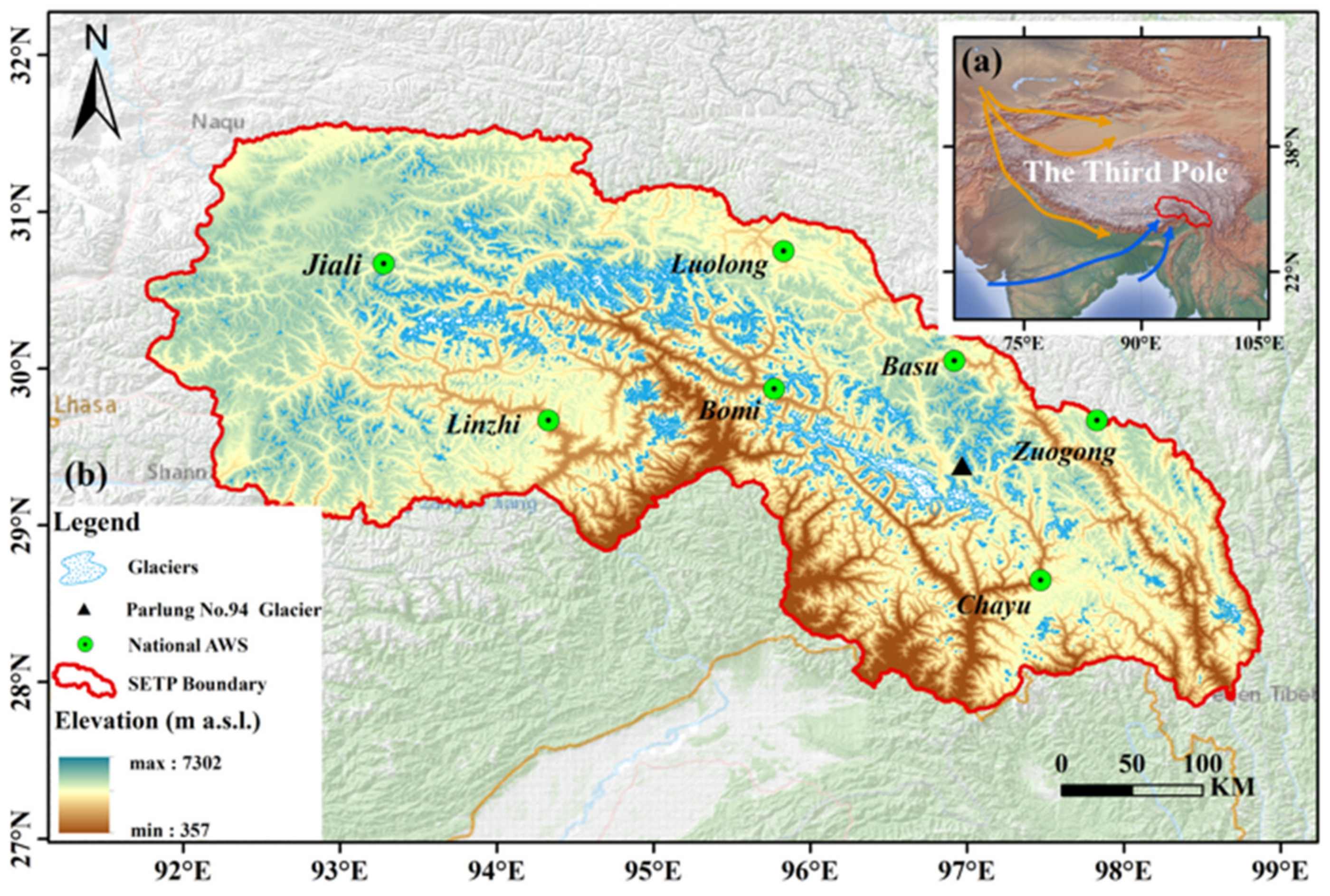
In this study, we employed the SETP boundary defined by Zhao [24]; this boundary encompasses clusters of glaciers within the SETP, with a particular focus on maritime glaciers. Notably, it includes the Eastern Himalayas, Eastern Nyainqêntanglha Ranges, and Western Hengduan Mountains. The SETP is a region known for its complex geological and topographic conditions. It has high mountains, deep valleys, and an average elevation of over 4000 m (Figure 1). Among these natural features, Nancha Barwa in the Eastern Himalayas stands out as the highest pinnacle. Meanwhile, the lower reaches of the Brahmaputra River have markedly lower elevations. In the SETP region, glaciers are predominantly found in the vicinity of the Parlung Tsangpo River basin. This river, which is a significant first-order tributary of the Brahmaputra, depends heavily on glacial meltwater for a substantial portion of its total flow. According to the RGI V6.0 glacier inventory [39], there are 7756 glaciers that collectively span 7260 km2. Of these glaciers, 95 have an area exceeding 10 km2, with a combined area of 2425 km2 (Table 1). The region also has a large number of small glaciers (with a glacier area smaller than 1 km2). However, despite their abundance, these small glaciers collectively account for less than 30% of the overall glacier area in the region.

Figure 1.
Map of the SETP region: (a) shows the SETP location in the Third Pole region, which is mainly influenced by the westerly winds (yellow curve and arrow) and the Indian summer monsoon (blue curve and arrow); (b) displays the distribution of glaciers and national weather stations, also including the location of Parlung No. 94 glacier.

Table 1.
Summary of SETP glacier area classification.
The SETP region, which is situated at the convergence region of the westerlies, Indian Ocean monsoon, and East Asian monsoon, benefits from a distinctive valley terrain [40,41]. This terrain fosters a unique water vapor channel, resulting in a large amount of precipitation within the SETP. In the Himalayas and Kangri Karpo Mountain of the SETP, the annual precipitation exceeds 1000 mm. Most of the precipitation in the SETP is concentrated between April and September, constituting approximately 80% of the total annual precipitation. Conversely, during the period from November to January, precipitation is relatively low, accounting for less than 5% of the yearly total. These precipitation patterns highlight the pronounced seasonal variability in the SETP, with most of the rainfall occurring during the warmer season and comparatively drier conditions during the winter season [41]. The mean annual temperature in the SETP region exhibits a declining trend from the southeast to the northwest. Our analysis of meteorological data spanning from 1980 to 2019 indicates a consistent upward trend in temperatures across the SETP. Notably, all stations experienced an increase of over 1 degree Celsius compared with the temperatures in 1980. Among these, the Chayu and Basu stations had an average annual temperature exceeding 10 degrees Celsius. However, the Jiali station recorded the lowest average annual temperature in the region.
Due to climate change in recent years, maritime glaciers are melting rapidly; this melting is further exacerbated by the region’s complex terrain, which frequently leads to glacier debris flows. Additionally, the formation of moraine lakes in the SETP significantly heightens the risk of glacier lake outburst floods (GLOFs) and other related glacial hazards [42].
3. Data and Methods
3.1. Datasets
3.1.1. Climate Datasets
In this study, we utilized the High Asia Refined analysis (HAR) v2 as the model’s baseline climate data [43]. The HAR v2 dataset is a regional atmospheric dataset that is generated through dynamical downscaling of the Final Operational Global Analysis (FNL) using the Weather Research and Forecasting (WRF) model. The dataset provides accurate and comprehensive gridded climate information for the high-mountain Asia (HMA) region, with a spatial resolution of 10 km. It has been successfully employed in various research fields, such as glacier mass balance modeling, snow analysis, and energy balance modeling [44,45]. One notable feature of the dataset is that it includes altitude data, enabling the computation of temperatures at specific elevations on glaciers. For each glacier, we extracted monthly time series data for temperature and precipitation from the nearest HAR v2 grid point. We then transformed these data points to local temperatures using a default temperature gradient of 6.5 K per kilometer. To account for the influence of changes in elevation, we used a precipitation correction factor (pf) to modify the HAR v2 precipitation time series. In our research, we calibrated the pf value based on the in situ mass balance of the Parlung No. 94 glacier. Through this calibration process, we determined that a pf value of 1.4 provided reliable results. To validate this calibration, we compared the correlation curve between winter precipitation and the pf value. Subsequently, we applied the calibrated pf value to every individual glacier in the SETP, which represented a regional adjustment to account for orographic precipitation, avalanches, and wind-blown snow.
For the projections, the sixth phase of the Coupled Model Intercomparison Project (CMIP6) data was used in this study; the CMIP6 was conducted under the organization of the World Climate Research Program (WCRP) [46], and the simulation data from previous phases of CMIP has been instrumental in enhancing our understanding of the climate and underlying mechanisms of climate change [47,48,49]. Here, we use gridded monthly precipitation and temperature data from four bias-corrected Global Climate Models (GCMs), which are GFDL-ESM4, MPI-ESM1-2-HR, UKESM1-0-sLL, and IPSL-CM6A-LR. For the data correction, we applied the anomaly method to these GCMs, specifically by using the “process_gcm_data” function to correct the model biases. The bias-corrected GCMs performed better than the original GCMs. Each GCM was associated with three shared socioeconomic pathways (SSP126, SSP370, and SSP585). SSP126 represents a future with aggressive climate action, limiting warming to 1.5 °C. SSP370 is an intermediate scenario with moderate action, leading to 2.0 °C to 3.0 °C warming. SSP585 depicts a high-emissions future with minimal action, resulting in over 4.0 °C of warming by 2100.
With regard to the selected models, the first two models are low climate sensitivity models and the latter two are high climate sensitivity models. We have seen these GCMs provide performance in previous studies focused on the Tibetan Plateau [50]; we acknowledge that different GCMs may have biases in the same region, but in this study, we mainly looked at the changes in the SETP glaciers under future scenario models, and thus, these GCMs we selected are good collections of the entire CMIP6 data.
We also used meteorological stations in our study area, which included 7 national automated weather stations (AWSs). The meteorological data could be used for the validation of the reanalysis data.
3.1.2. Glacier Mass Balance Data
The geodetic estimates provided by Hugonnet et al. served as the primary reference for the global studies in this research [3]; owing to their broad accessibility worldwide, they constitute a crucial dataset that was utilized for calibration and validation purposes throughout the study. We used the new calibration method in OGGM v1.6 (for details, see Section 3.2.5). The geodetic data for each glacier in the SETP has three periods: 2000–2020s, 2000–2010s, and 2010–2020s. The geodetic mass balance data were period averaged; we used the period 2000–2020s data for calibration and the other two periods for validation. Furthermore, within the WGMS dataset [25], only about 300 glaciers have in situ glaciological observations that offer higher spatial and temporal resolution globally. In the SETP, there is only the Parlung No. 94 glacier that has long-term mass balance observations documented in the WGMS dataset, with the mass balance time series from 2006–2018 being employed for the model validation.
3.1.3. Ancillary Data Sets
In this study, the OGGM model utilized glacier outlines sourced from the Randolph Glacier Inventory v6 (RGI v6), which was published in 2017 [39]. These outlines, which are provided by the Global Land Ice Measurements from Space (GLIMS), were employed for the initial topographical processing within the model. Furthermore, the NASADEM was used to derive elevation-band flowlines. The NASADEM dataset, which is available at a resolution of one arc-second, can be obtained from the land Processes Distributed Active Archive Center (LP DAAC) via NASA Earth data [51]. This dataset was downloaded and then interpolated onto the local grid based on the specific glacier location and outline. NASADEM is an enhanced version of the DEM and is derived from data collected by the Shuttle Radar Topography Mission (SRTM). Compared with other elevation datasets, NASADEM offers higher resolution, making it invaluable for projects that require high-resolution elevation data.
To estimate the ice thickness, the OGGM utilized the mass conservation approach, which assumes that the glacier outline and DEM correspond to the same date. In this study, the creep parameter A and slide parameter f were calibrated on an individual basis for each glacier to align with the ice volume estimates provided by Farinotti and others [2] at the RGI year (for many glaciers, this was close to 2000).
3.2. Methods
3.2.1. Open Global Glacier Model Description
The OGGM was utilized in this study for the purpose of reconstructing the glacier mass balance and simulating glacio-hydrological processes. The model demonstrates the ability to simulate glacier dynamics through the implementation of the shallow ice approximation, which allows for the calculation of depth-integrated ice flux along multiple flow lines. Additionally, it is capable of simulating key glacier characteristics, including mass balance (the equilibrium between ice accumulation and loss), ice thickness estimation, and capturing the dynamic behavior of glaciers over time [32]. In this research, the updated OGGM version 1.6 was employed, which offers a new calibration method in comparison to previous versions [52].
The glacier mass balance module in the OGGM is the updated version of the temperature index model developed by Marzeion [53]. The monthly glacier mass balance at an elevation z was estimated using Equation (1):
is the solid precipitation (kg m−2 month−1); is the air temperature at the altitude z; and is the temperature at which ice melt occurs, where we set = −1 °C. The proportion of solid precipitation was represented as a percentage of the total precipitation. It was considered to be 100% solid when the temperature () was equal to or below the solid temperature threshold () of 0 °C, and 0% when the temperature was equal to or above the liquid temperature threshold () of 2 °C. The percentage of solid precipitation was linearly interpolated for temperatures between and . is the degree-day factor of glaciers (kg m−2 K−1 month−1). The fraction of solid precipitation was estimated from the monthly or daily mean temperature. Precipitation was assumed to be entirely solid below 0 °C and all liquid above 2 °C. In between, the solid precipitation proportion changed linearly.
Three parameters were used to characterize our temperature index model variants. In addition to the degree-day factor (also known as “melt_f”), which represents the degree-day factor of glaciers, two parameters are commonly included in the temperature index model. However, these parameters actually serve as tools for local climate downscaling or bias correction. The precipitation was adjusted using a fixed multiplicative scaling precipitation factor (pf), and the temperature was corrected using a temperature bias (“temp_bias”). These parameters were crucial because the model would often fail to reproduce the observed glacier mass balance without them. It is important to note that these model parameters not only served as downscaling parameters but also accounted for local climate biases, incorporated missing mass balance processes (such as debris cover and avalanches), and addressed inaccuracies in mass balance observations. To downscale the temperature and precipitation data for each elevation band in our temperature index model, we utilized a temperature lapse rate and downscaled the data from the nearest grid point.
3.2.2. Model Spin-Up
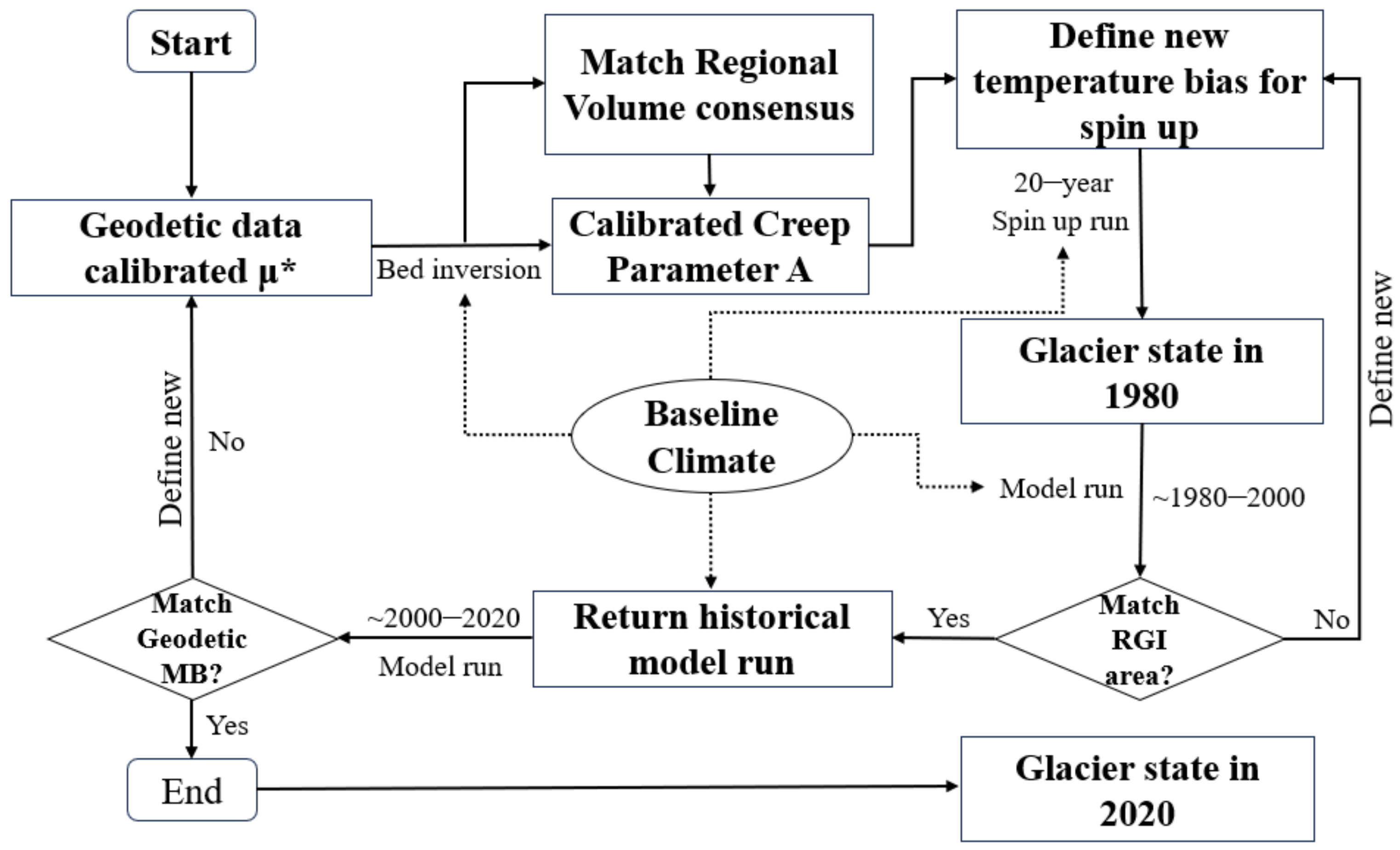
Before reconstructing the historical glacier mass balance, we performed a dynamical spin-up using historical climate data. This allowed the glacier to grow to its size at the RGI date. Additionally, a dynamical initialization helped to remove strong assumptions in the OGGM default settings. These assumptions included the idea that glaciers are in dynamical equilibrium at the glacier outline date (which is required for the ice thickness inversion) and that the mass balance melt factor parameter (“melt_f”) is calibrated based on geodetic mass balance, without taking into account the dynamically changing glacier geometry. The main dynamical spin-up methods are introduced as follows (Figure 2).
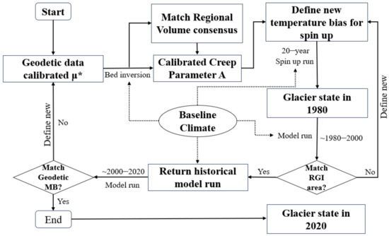
Figure 2.
OGGM spin-up flowchart. The μ* is glacier sensitivity parameter, RGI denotes the Randolph Glacier Inventory version 6.0.
First, we defined a glacier sensitivity parameter (μ*); μ* is defined by matching the modeled mass balance with the geodetic mass balance of Hugonnet et al. [3]. Then, we calculated the apparent mass balance using a static geometry and baseline climate in the geodetic mass balance period; this procedure found a mass balance residual to add to the 2000–2020 mass balance profile so that the average mass balance was equal to 0, hence following the equilibrium assumption. Second, we used the apparent mass balance for an inversion of the underlying glacier bed. Using this inversion, the creep parameter A was defined and the resulting inversion glacier volume matched the regional volume estimate by Farinotti et al. [2]. The inversion method follows Maussion et al. [32] and the sliding parameter was set to 0. Third, we ran a dynamical spin-up to find the glacier state in 1980, we assumed the RGI data were from 2000 (mostly they were from around 2000). To define the different glacier states in the past, the temperature bias for the spin-up was added to the baseline climate during a 20-year constant mass balance run (the first guess was −1 °C), and the constant mass balance was given by the baseline climate between 1980 and 2000. We only moved on if this step successfully found a proper past glacier state to match the RGI area within 1 km2. Then, we ran a dynamic simulation from 1980 to 2020 using the baseline climate inputs and starting from the past glacier state we obtained. Finally, we used the model to calculate the 2000–2020 mass balance and compared it with the geodetic values from Hugonnet et al. If the result matched the geodetic values, the calibration was terminated and the resulting glacier in 2020, the creep parameter A, and μ* were used as the inputs for the projection runs. If not, the newly defined μ* was used to run the whole process again. After the model spin-up, we obtained the past state of glaciers and the glacier state in 2020; then, we could use GCMs to drive the model to simulate glacier change after the 2020s.
3.2.3. Glacier Runoff Simulations
In OGGM v1.6, the “run_with_hydro” task was utilized to calculate the glacier runoff. In the OGGM, the glacier runoff outputs are computed for the largest area that was occupied by the glacier ice throughout the simulation period. The simulated glacier runoff consists of four individual components: melt on-glacier, melt off-glacier, liquid precipitation on the glacier, and liquid precipitation off the glacier. The melt on the glacier comprises both ice melt and seasonal snow melt; the melt off the glacier melts due to the seasonal snow accumulation in a reservoir, providing off-glacier meltwater during the summer months from the stored snow, extending beyond the glacier into non-glacial areas; the liquid precipitation equals the rainfall on glacier plus rainfall off the glacier. The total glacier runoff is calculated using Equation (2):
Similarly, the variable α signifies the sum of ice melting taking place on the glacier and the combined snow melt occurring both on and off the glacier, and represents the contribution of liquid precipitation from both on and off the glacier areas. These values, namely, α and , are calculated from the glacier mass balance model (Equation (1)). Therefore, to simulate the glacier runoff based on the maximum extent of the glacier and to ensure that the cumulative runoff does not exceed the annual volume change, certain measures are taken. The mass balance model utilized in the OGGM applies the principle of mass conservation to estimate the different components of glacier runoff, including rainfall and melt runoff.
3.2.4. SETP Glacier Mass Balance Calculation Method
To account for the variations in scale and size between different glaciers, a more accurate calculation of the mass balance for the SETP was performed by considering the mass balance of the weighted area. This calculation was based on a single glacier scale and can be expressed using Equation (3):
where represents the average annual mass balance of the first glacier, represents the area of this glacier, represents the annual average mass balance of the nth glacier, and represents the area of the nth glacier. This approach considers the contribution of each glacier relative to its size or area. By incorporating the weighted area concept, the calculation yields more precise results.
3.2.5. Model Calibration and Validation
In this study, we utilized a novel calibration method introduced in OGGM v1.6 [52]. Before version 1.6, the OGGM employed a relatively basic calibration approach that utilized data from a few hundred in situ observations of glaciers for model calibration. It then utilized an interpolated parameter called “t_star” for glaciers lacking direct observations [32]. This method was found to be highly effective, though it does have specific limitations. With the availability of new observational datasets, we can now perform glacier calibration on an individual basis. In this study, we utilized the geodetic glacier mass balance dataset provided by Hugonnet et al. [3]. The calibration method employed in this study followed the “three-step” calibration approach proposed by Hock and others [54].
First, we utilized in situ observation data from the Parlung No. 94 glacier to calibrate the precipitation parameter (pf). By keeping the other two parameters, namely, the temperature sensitivity parameter (“melt_f”) and the temperature bias parameter (“temp_bias”) fixed, we focused on calibrating the precipitation parameter (pf) independently. We discovered that setting pf to 1.4 resulted in a significant alignment between the model simulation data and the measured data. Given that the SETP region experiences substantial winter precipitation in comparison with other regions in high-mountain Asia, we conducted further analyses to validate the rationality of the chosen precipitation parameter (pf) value. Specifically, we compared the linear relationship curve between winter precipitation and precipitation parameters to confirm its significance. We applied the calibrated precipitation parameters (pf) to each glacier within the SETP region for our study. Second, after fixing the precipitation parameter (pf) at its previously determined value, the calibration of the other two parameters was carried out sequentially; before the calibration, the temperature bias parameter (“temp_bias”) was set in a reasonable range, typically ranging from −15 to 15, and the temperature sensitivity parameter (“melt_f”) was set in the range of 1.5 to 17. During the calibration process, we calibrated a total of 7756 glaciers; only a small subset of glaciers showed signs of over-parameterization. In response to this, we adjusted the parameter ranges to ensure a fit.
Regarding model validation, we first conducted the model simulation and validations on the observed glacier (Parlung No. 94 glacier) at different scales, including the elevation scale and glacier scale. Second, at the regional level, we compared the results of the model with the geodetic measurement dataset.
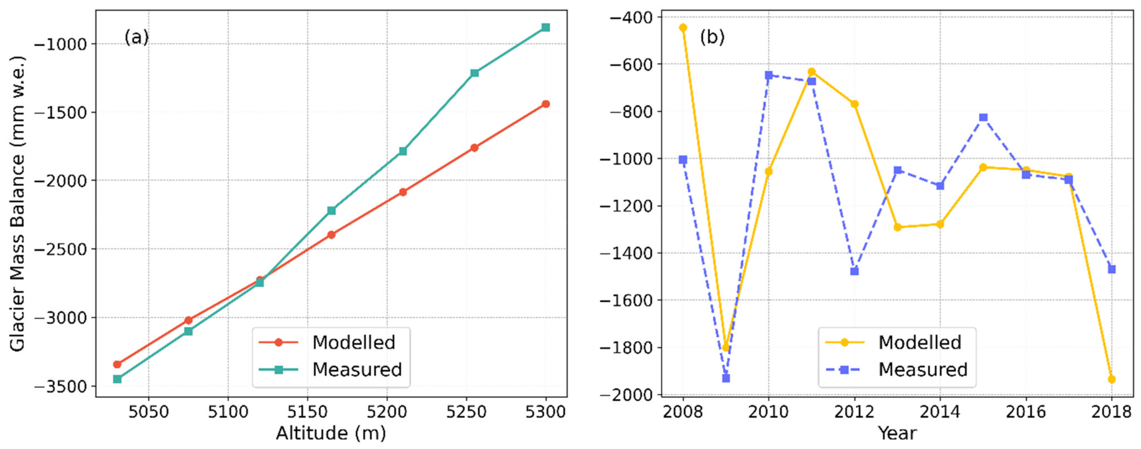
On the elevation scale, to evaluate the simulation performance of the model, data from the Parlung No. 94 glacier measured between 2006 and 2018 were utilized. The stakes of the glacier are mainly found at altitudes ranging from 5000 m to 5300 m. To enhance the accuracy of representing the glacier’s mass balance relative to altitude, we segmented the data into four altitudinal zones: 5030–5100 m, 5100–5200 m, 5200–5300 m, and above 5300 m. For altitudes exceeding 5300 m, we considered only a single data point, whereas each of the other specified zones encompassed two data points. Utilizing the OGGM model, we computed the average mass balance for each altitude zone over the period from 2006 to 2018. A comparative analysis between the simulated mass balance for each altitude zone and the corresponding measured values yielded a correlation coefficient of 0.997. This high correlation underscored the calibrated model’s proficiency in replicating the altitude-dependent gradients of the glacier, as depicted in Figure 3.
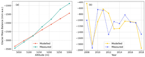
Figure 3.
Validation of Parlung No. 94 glacier: (a) denotes the validation of the altitude gradient, comparison between the in situ measurement, and simulation of the mass balance of Parlung 94 glacier at 5030–5300 m from 2006 to 2018, and (b) shows comparison between the in situ measurement and simulation of the mass balance of Parlung 94 glacier.
Furthermore, the annual mass balance simulated by the model exhibited consistency with the measured data in terms of trend. However, it is crucial to note that the annual mass balance represents the average value computed from a limited number of altitude data points with stakes rather than a comprehensive statistical mass balance encompassing the entire glacier altitude range. Overall, the calibrated model showed exceptional performance in simulating the altitude gradients and annual mass balance of the Parlung No. 94 glacier. The strong correlation with the measured data confirmed its accuracy in representing the glacier’s behavior.
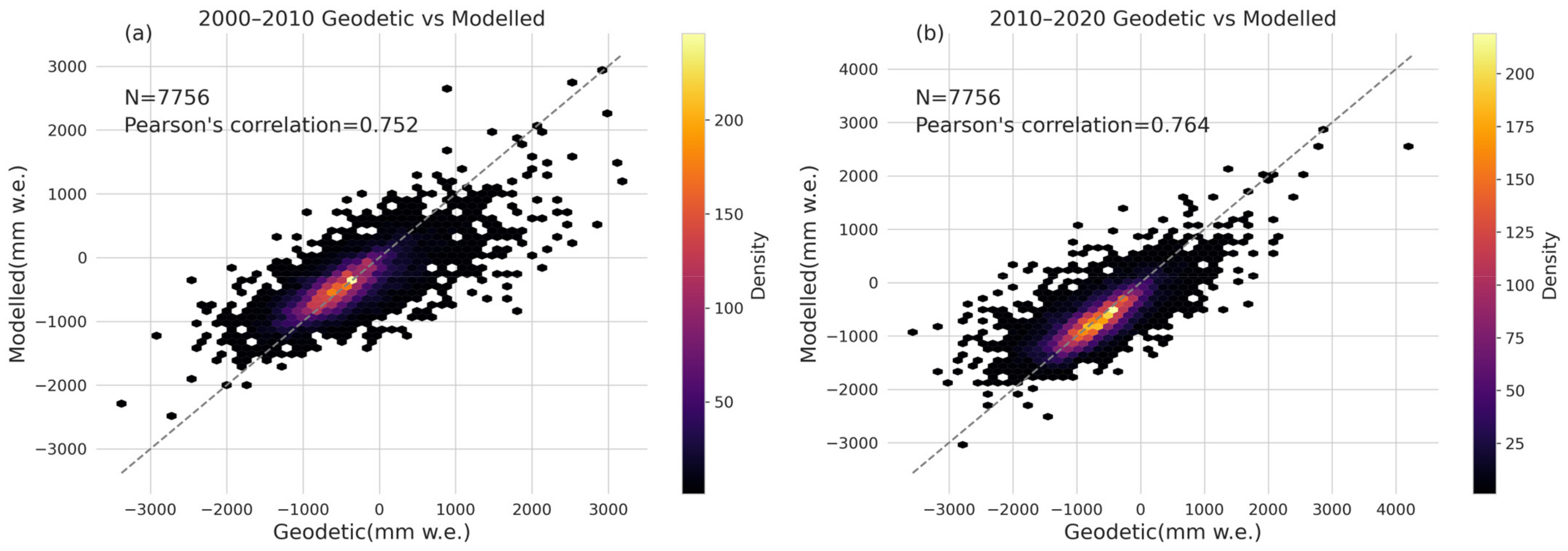
On the regional scale, the calibrated model was applied to simulate a larger set of 7756 glaciers in the SETP (Figure 4). The average mass balance of each glacier was simulated for two time periods: 2000–2010s and 2010–2020s. To validate the simulation results, the geodetic dataset corresponding to each glacier was extracted and compared with the model’s outputs. Comparing the simulation results of the calibrated model with the geodetic data, the Pearson correlation coefficients for the two time periods were found to be 0.752 and 0.764, respectively. These correlation coefficients indicate a moderately strong positive relationship between the model’s simulated mass balance and the geodetic data for both periods. This analysis confirmed that the calibrated model not only performed well in simulating the behavior of a single glacier in terms of altitude zones and annual mass balance but also exhibited a good simulation performance when applied to a regional scale.
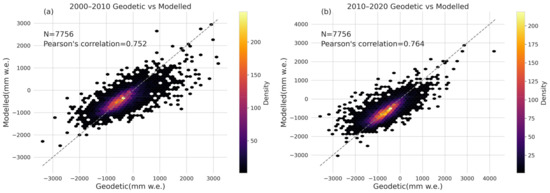
Figure 4.
The comparison between the calibrated model simulation results and the geodetic results: (a) is the comparison between the 2000–2010 simulation results and the 2000–2010 geodetic data, and (b) is the comparison between the 2010–2020 simulation results and the 2010–2020 geodetic data.
4. Results
4.1. Glacier Mass Balance
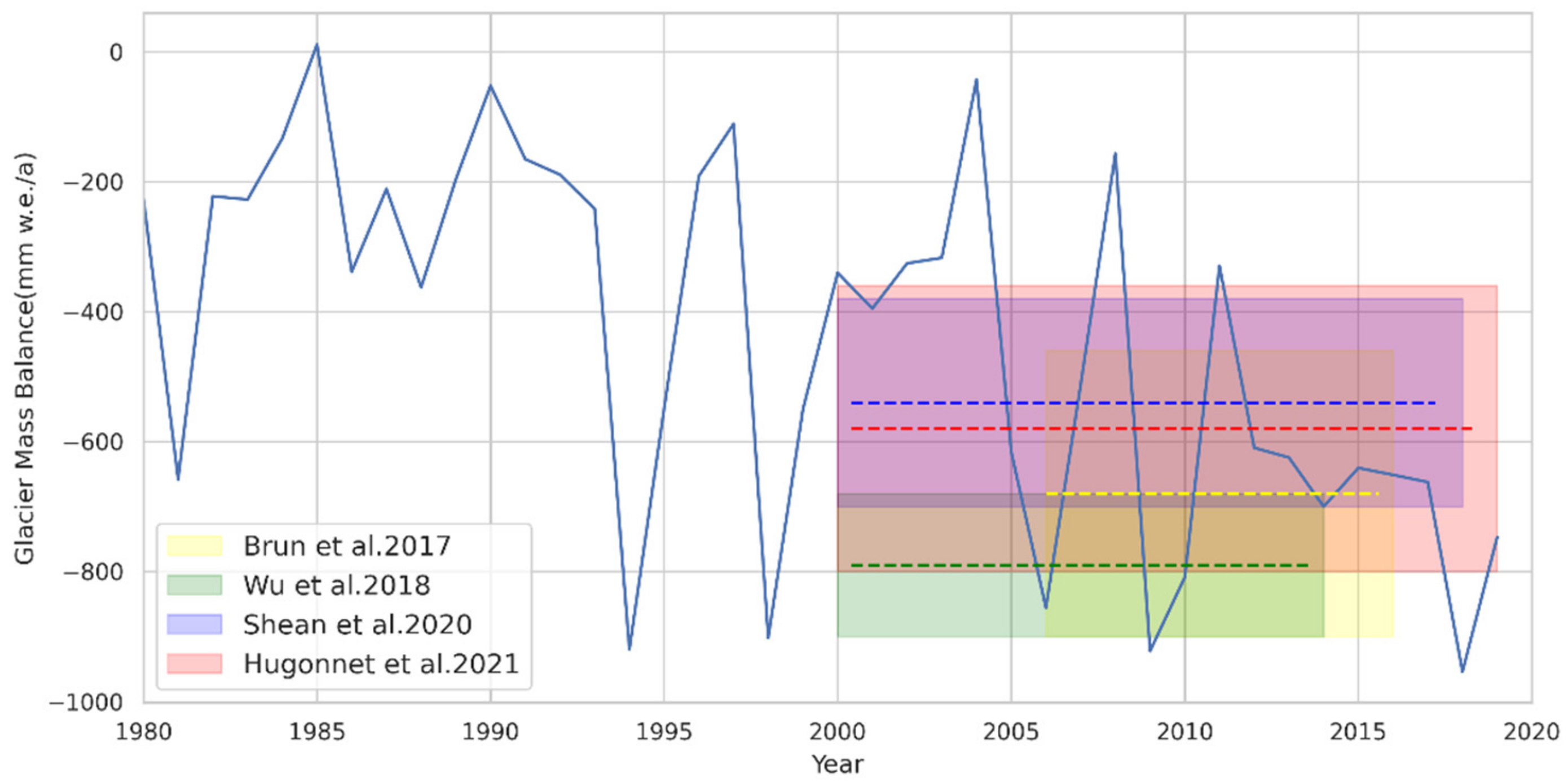
The mass balance of glaciers is a crucial indicator for assessing their overall health. In the region of the Third Pole, specifically the SETP, glaciers have been experiencing serious loss. It is of utmost importance to understand the detailed changes occurring in these glaciers. To investigate this, a model was utilized to calculate the mass balance of each glacier in the SETP region from 1980 to 2019. However, it is important to consider that large and small glaciers contribute differently to the regional glacier mass balance. Considering the varied influences of different glacier sizes on the calculation of the regional mass balance, a weighted area method (Equation (3)) was employed. Based on the calculations, the mass balance of glaciers in the SETP region for the research period from 1980 to 2019 was estimated to be −0.50 ± 0.28 m of water equivalent per year (m w.e. a−1). Further analysis focused on the mass balance of glaciers over the past two decades, revealing a mass balance of −0.38 ± 0.25 m w.e. a−1 from 1980 to 1999 (Figure 5). The results indicate a rapid loss trend in the SETP glaciers since the beginning of the 21st century. We also compared the modeling results with several mainstream geodetic observations in the SETP [3,11,12,55], our result has good consistency with these studies.

Figure 5.
Time series of SETP glacier mass balance and comparison with several sets of geodetic data products after 2000 [3,11,12,55].
Specifically, the model simulations showed that the mass balance of glaciers in the SETP region from 2000 to 2019 was −0.62 ± 0.24 m w.e. a−1. Breaking it down further, the mass balance from 2000 to 2009 was −0.53 ± 0.27 m w.e. a−1, while from 2010 to 2019, it accelerated to −0.71 ± 0.15 m w.e. a−1. This analysis revealed the significant negative mass balance of the SETP glaciers, indicating substantial ice loss over the research period.
4.2. Spatial Variability in Glacier Mass Balance
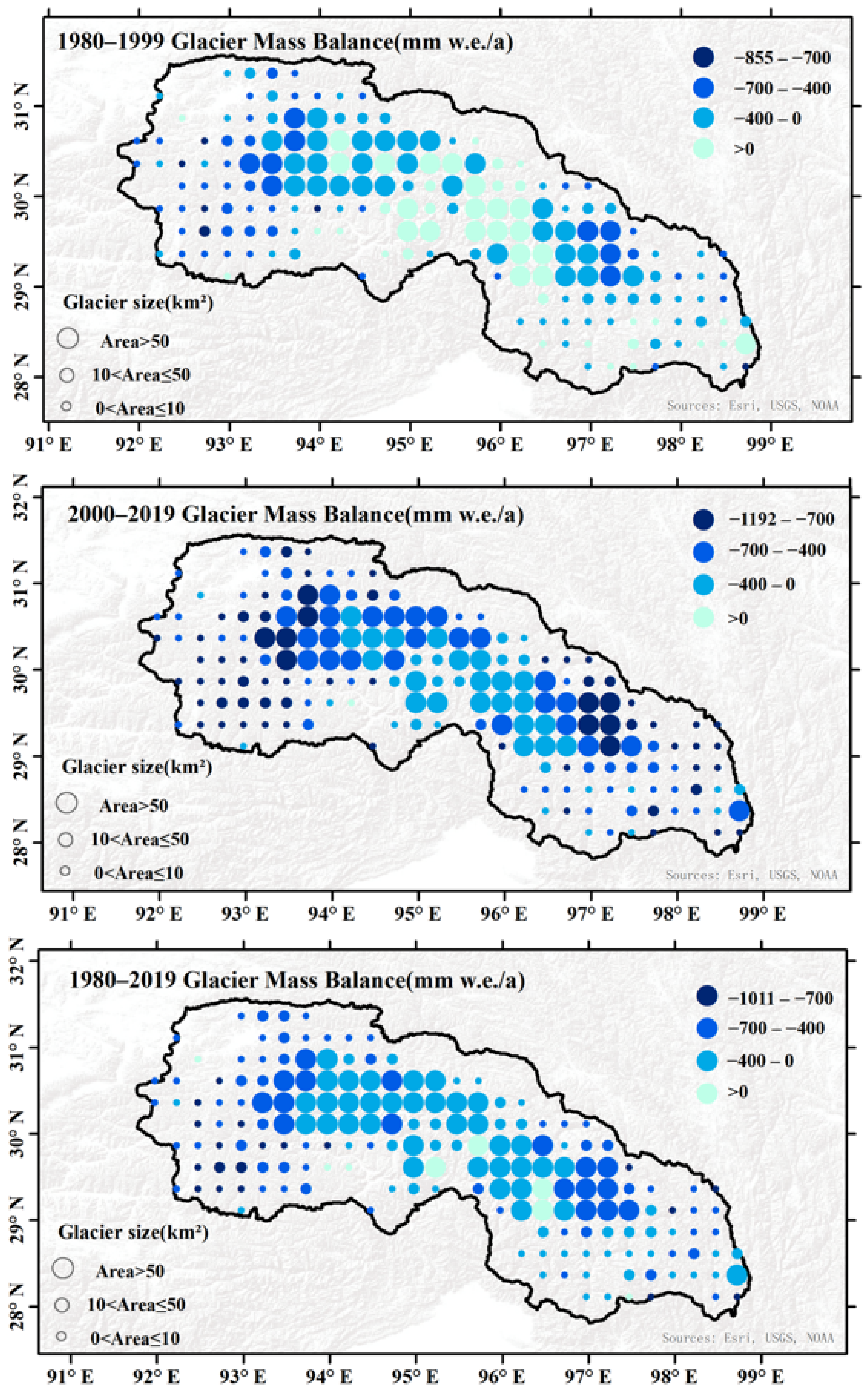
In this study, we classified the calculated mass balance of glaciers into different periods and computed the spatial variation characteristics of the SETP glaciers using 0.25° × 0.25° grid cells. To comprehend the spatial variation characteristics of the historical mass balance of glaciers at different locations and sizes in the SETP, we categorized the glacier area into three groups: 0 < area < 10 km2, 10 < area ≤ 50 km2, and area > 50 km2. The classification of glacier sizes was determined based on the size of the glacier area within each grid cell and was represented using four different colors to depict the range of glacier changes (Figure 6). This approach provided insights into the approximate distribution of glacier sizes in the SETP and how the historical mass balance of glaciers within these size categories has evolved. The classification of glacier sizes revealed that the largest concentration of glaciers is situated in the central part of the SETP, extending toward the east and west. As one moves toward the boundaries of the SETP, the glaciers gradually decreased in size.
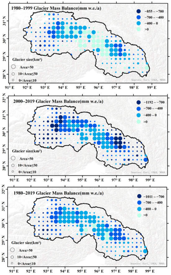
Figure 6.
Spatial variation of glacier mass balance in the SETP at 0.25° × 0.25° grid scale; 1980–1999s, 2000–2019s, and 1980–2019s are shown.
Regarding the spatial distribution of the glacier mass balance, the simulation results of the model indicate that there was a positive balance distribution of glaciers in the middle of the SETP from 1980 to 1999, but the northwestern and southeastern regions of the SETP exhibited a rapid loss. There were small-scale clusters of glaciers found in the western basin, which experienced the most severe loss in the SETP during this time, reaching up to −0.85 m w.e. a−1. Analyzing the spatial variation of the SETP mass balance during this period, it could be determined that from the central part of the glacier to the east and west, the glacier underwent stepwise depletion, extending toward the northwest and southeast regions, which experienced the most significant mass loss among the SETP glaciers. By examining the spatial changes in the SETP glaciers from 2000 to 2019, the same pattern could be observed: the central clusters of the SETP glaciers represented an area with relatively small mass loss, extending from the central part to the east and west sides, demonstrating a gradient effect of accelerated loss. The northwestern and southeastern regions of the SETP experienced the most severe loss of glacier mass balance.
After analyzing the spatial variations in the mass balance of the glaciers in the SETP, our primary focus was on examining the change rate of these glaciers. A comparison of the data from two distinct periods, namely, 1980–1999 and 2000–2019, revealed that since the beginning of the 21st century, the glaciers in the SETP experienced accelerated loss. This change was evident from both the changes in color and the spatial distribution of the average glacier mass balance over the two 20-year periods. The most significant changes were observed in the central part of the SETP, where the largest cluster of glaciers was located. Due to its location in the core area of maritime glaciers and its surrounding terrain and glaciers, the central glaciers experienced the least amount of mass loss. We found that a significant portion of the average mass balance of these central glaciers was positive from 1980 to 1999. However, when entering the 21st century, all the glaciers in the central part with a positive mass balance shifted to a negative balance during 2000–2019. On the northeastern and southwestern sides of the SETP, the glaciers that initially had a negative mass balance showed a further deepening in color, indicating that an intensified loss of glaciers happened during the 21st century.
4.3. Future Dynamics of Maritime Glaciers
Glacier dynamics are characterized by the delayed responses of glaciers to climate change. In this study, we projected the dynamic responses of the SETP glaciers to future climate change using four GCMs and three SSPs (SSP126, SSP370, SSP585).
The SETP boundary contains three basins; in this study, we focused on partial basins within the SETP. We established a boundary that included three major river basins: the Brahmaputra Basin, Salween Basin, and Mekong Basin. According to Table 2, the Brahmaputra Basin, which is situated within the boundary of the SETP, encompassed a total of 6192 glaciers, accounting for 86.6% of the glacier area. Similarly, the Salween Basin contained 1514 glaciers, representing 12.6% of the total glacier area. On the other hand, the Mekong Basin, held only 50 glaciers, amounting to 0.8% of the total glacier area.

Table 2.
Statistics of glaciers in the three major river basins within the boundaries of SETP.
In order to assess the future change characteristics of glaciers in these three major basins within the SETP boundary, we divided the SETP into three parts using the basin boundaries. We then employed a data-driven model based on the GCMs to simulate the glaciers in each respective basin within the SETP from 2020 to 2100. Specifically, we focused on dynamic characteristics, such as the glacier length, glacier area, and glacier volume.
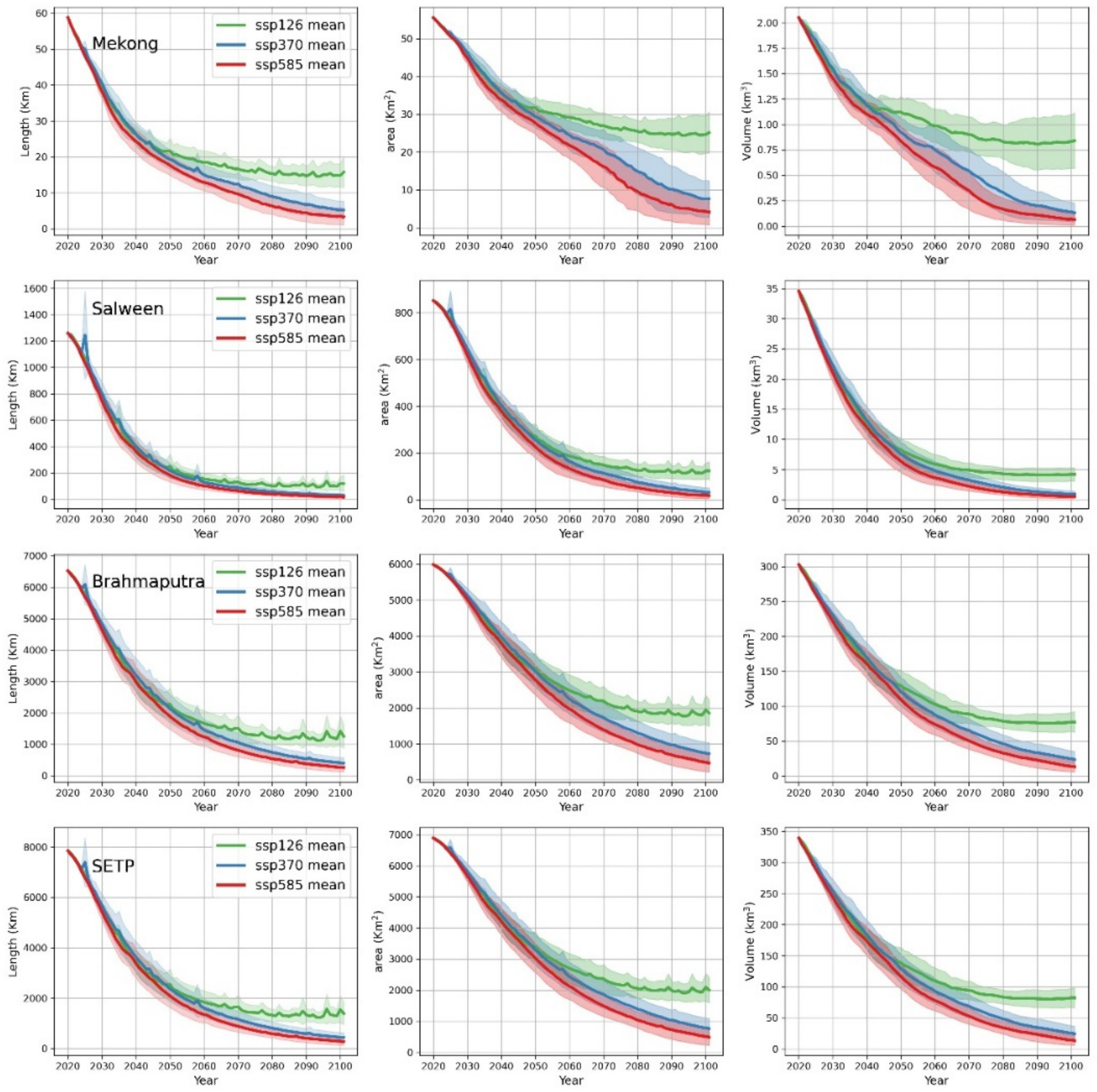
The simulation results (Figure 7) project significant changes in the glaciers of the Mekong, Salween, and Brahmaputra Basins within the SETP region from 2020 to 2100, considering averages across multiple models and various SSP scenarios. In the Mekong Basin, which holds a small proportion of the SETP glaciers, it was estimated that toward the conclusion of the 21st century, the glacier area will have decreased by approximately 78.01% ± 6.25%, the length by 86.59% ± 4.36%, and the volume by 83.1% ± 6.83%. Moving to the Salween Basin, the projections suggest a disappearance of about 95.03% ± 3.17% of the glacier area, a shrinkage of 95.50% ± 2.36% in length, and a decrease of 94.58% ± 2.60% in volume by the close of the 21st century. In the Brahmaputra Basin, the glacier area is expected to vanish by approximately 82.28% ± 5.07%, the length to decrease by 89.27% ± 4.46%, and the volume to decline by 87.32% ± 4.63% toward the conclusion of the 21st century. Considering the entire SETP area, the projections indicate an overall reduction in the glacier area by about 83.57% ± 4.91%, length by 90.25% ± 4.23%, and volume by 88.04% ± 4.52% toward the conclusion of the 21st century. These findings underscore substantial and concerning declines in the glacier extent, length, and volume across the SETP region in the coming decades.
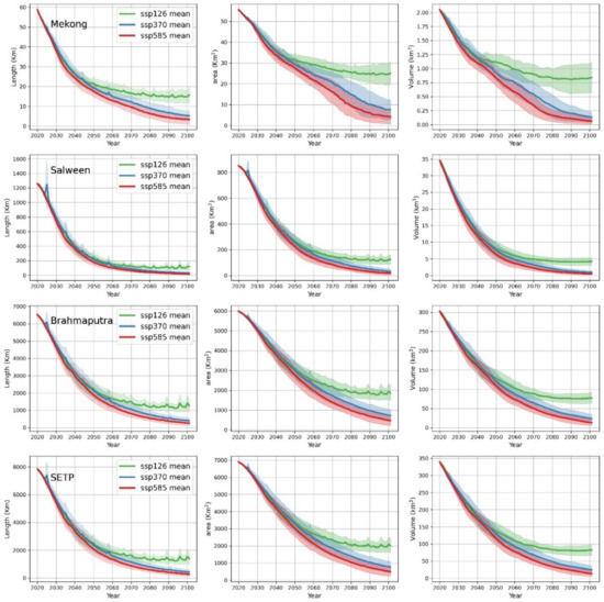
Figure 7.
Glacier dynamics (length, area, volume) prediction results from 2020–2100 within the three major basins located in SETP (Mekong Basin, Salween Basin, Brahmaputra Basin) and the whole SETP, the shaded part represents one standard deviation.
4.4. Future Glacier Runoff Components Estimation
We analyzed the components of the glacier runoff, which included the precipitation runoff and the glacier melt runoff resulting from glacier ablation. To assess the future change trend in the glacier melt runoff from 2020 to the end of the century, we employed the same methodology used for calculating the glacier dynamic components. We utilized a multi-model and multi-SSP scenario averaging approach to obtain more robust predictions.
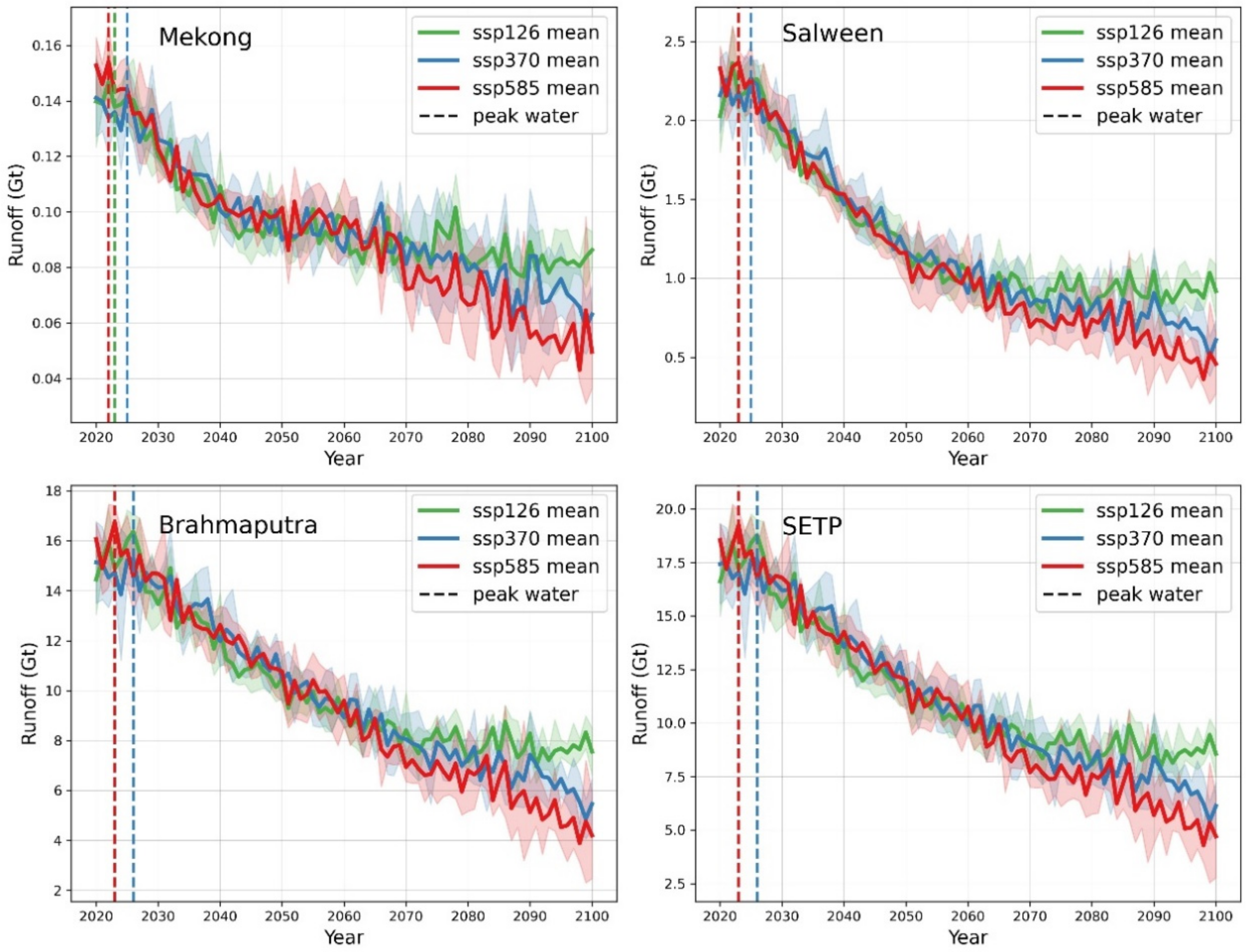
According to our findings (Figure 8), by the end of this century, the runoff from glaciers in the Mekong Basin was projected to decrease by approximately 57.14% with a variability range of ±14.29%. Similarly, the glacier runoff in the Salween Basin is expected to decrease by around 67.32%, with a variability range of ±6.90%. In the Brahmaputra Basin, the projected decrease in glacier runoff will be approximately 61.77%, with a variability range of ±4.37%. Overall, toward the conclusion of the 21st century, the SETP region is anticipated to experience a significant reduction in glacier melting runoff, which is estimated to be around 62.63% with a variability range of ±6.16%. Our study predicted that the runoff resulting from the melting of glaciers in the SETP region will substantially decrease over the course of this century. This has significant implications for the water resources and overall hydrology of the Mekong, Salween, and Brahmaputra Basins.
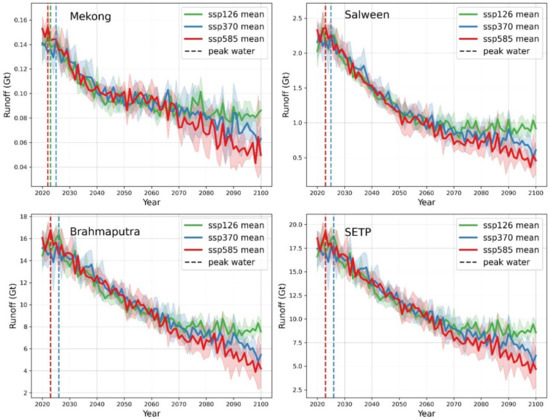
Figure 8.
Glacier melt runoff prediction of three basins and SETP from 2020 to 2100 based on the ensemble average of multiple GCMs and considering different SSPs, the shaded part represents one standard deviation. Furthermore, we estimated the timing of the “peak water” point in these basins and SETP.
The “peak water” point of glacier melt runoff is a crucial indicator that helps us understand the fate of glaciers. In our study, we calculated the changing characteristics of glacier runoff under different SSP scenarios by considering multiple GCM sets for each basin. We focused on estimating the “peak water” point, which refers to the year when the glacier runoff will reach its maximum before declining.
In the Mekong Basin, our estimations suggest that under the SSP126 scenario, the peak water point for glacier runoff will occur in 2023. Under the SSP370 scenario, it will happen in 2025, and under the SSP585 scenario, it is expected to occur in 2022. Moving to the Salween Basin, our predictions indicate that under the SSP126 scenario, the peak water point for glacier runoff will occur in 2023. Under the SSP370 scenario, it is projected to occur in 2025, while under the SSP585 scenario, it is estimated to happen in 2023. Interestingly, the SSP126 and SSP585 scenarios shared the same peak water year in the Salween Basin. In the Brahmaputra Basin, our projections suggest that under the SSP126 scenario, the peak water point for glacier runoff will arrive in 2026. Under the SSP370 scenario, it is also expected in 2026, while under the SSP585 scenario, it is anticipated to occur in 2023. Similarly, in the Brahmaputra Basin, the peak water years were the same for the SSP126 and SSP370 scenarios. Considering the entire SETP region, we estimated that the peak water point for glacier runoff will occur in 2026 under the SSP126 and SSP370 scenarios. However, under the SSP585 scenario, the peak water point was predicted to occur earlier, specifically in 2023.
Precipitation runoff is another important runoff source. The future precipitation projections in the SETP showed an overall increase trend; this is consistent with a previous study that indicates the SETP will have the most future precipitation in the Tibetan Plateau [50]. For three basins in the SETP, their precipitation runoff showed a consistent increase trend. As the time moved to the 2060s, the precipitation in the SETP showed a predicted accelerating upward trend, but the standard error was enlarging at the same time (Figure 9).
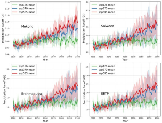
Figure 9.
The precipitation runoff prediction of three basins and SETP from 2020 to 2100 based on the ensemble average of multiple GCMs and considering different SSPs; the shaded part represents one standard deviation.
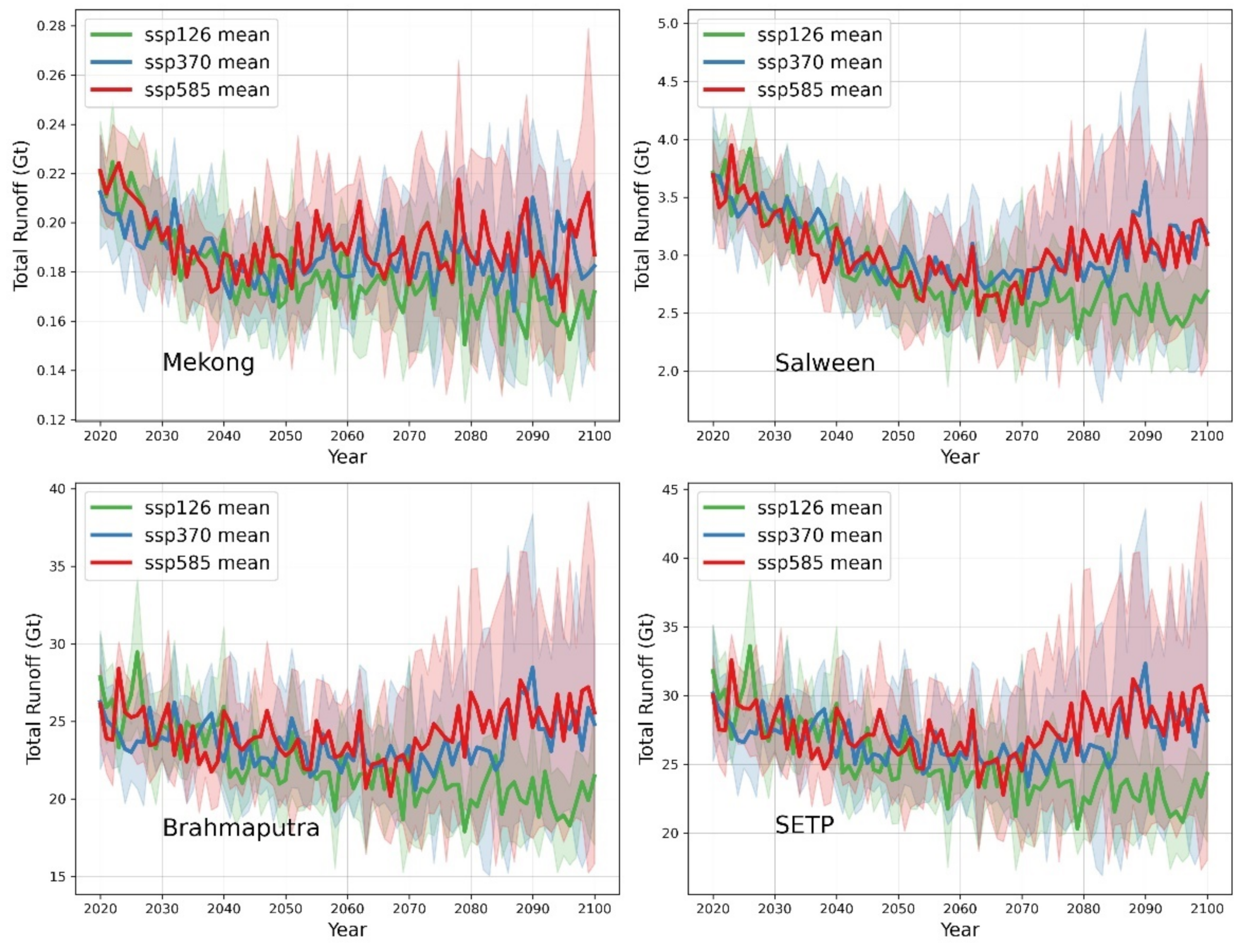
In the future, the increase in precipitation is expected to offset the rapid decline in glacier melt runoff. As Figure 10 illustrates, for basins with fewer glaciers, there will be a faster declining trend in the total runoff (which includes both the glacier melt and precipitation runoff). In contrast, basins with a larger number of glaciers will exhibit a more stable declining trend in total runoff. Over time, as glaciers increasingly recede and the contribution from glacier melt becomes unsustainable, a rapid downward trend in runoff is anticipated, eventually stabilizing. For the entire SETP, the decline in total runoff will be mitigated by increased precipitation. The total runoff in the SETP is projected to reach its lowest point between the 2060s and 2070s, followed by a gradual increase, peaking in the 2090s, and then demonstrating a slight declining trend. Overall, the total runoff trend in the SETP is expected to remain relatively stable, fluctuating between 20 and 30 GT under the three ensemble scenarios.
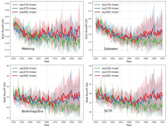
Figure 10.
The total runoff prediction of three basins and SETP from 2020 to 2100 based on the ensemble average of multiple GCMs and considering different SSPs; the shaded part represents one standard deviation.
5. Discussion
5.1. Glacier Mass Balance Sensitivity Experiments
Glacier sensitivity, which is a crucial metric in cryosphere studies, quantifies the responsiveness of glaciers to climatic variations. The SETP is located at the confluence of the Indian Ocean summer monsoon, westerly wind, and East Asian monsoon, making it a region that is highly sensitive to the effects of climate change. For the HMA, researchers have investigated the HMA glaciers’ sensitivity to temperature and precipitation [56]. However, the time span is short and the data resolution is coarse; with regard to the rapid mass loss in the SETP, longer-period and higher-resolution sensitivity experiments are needed.
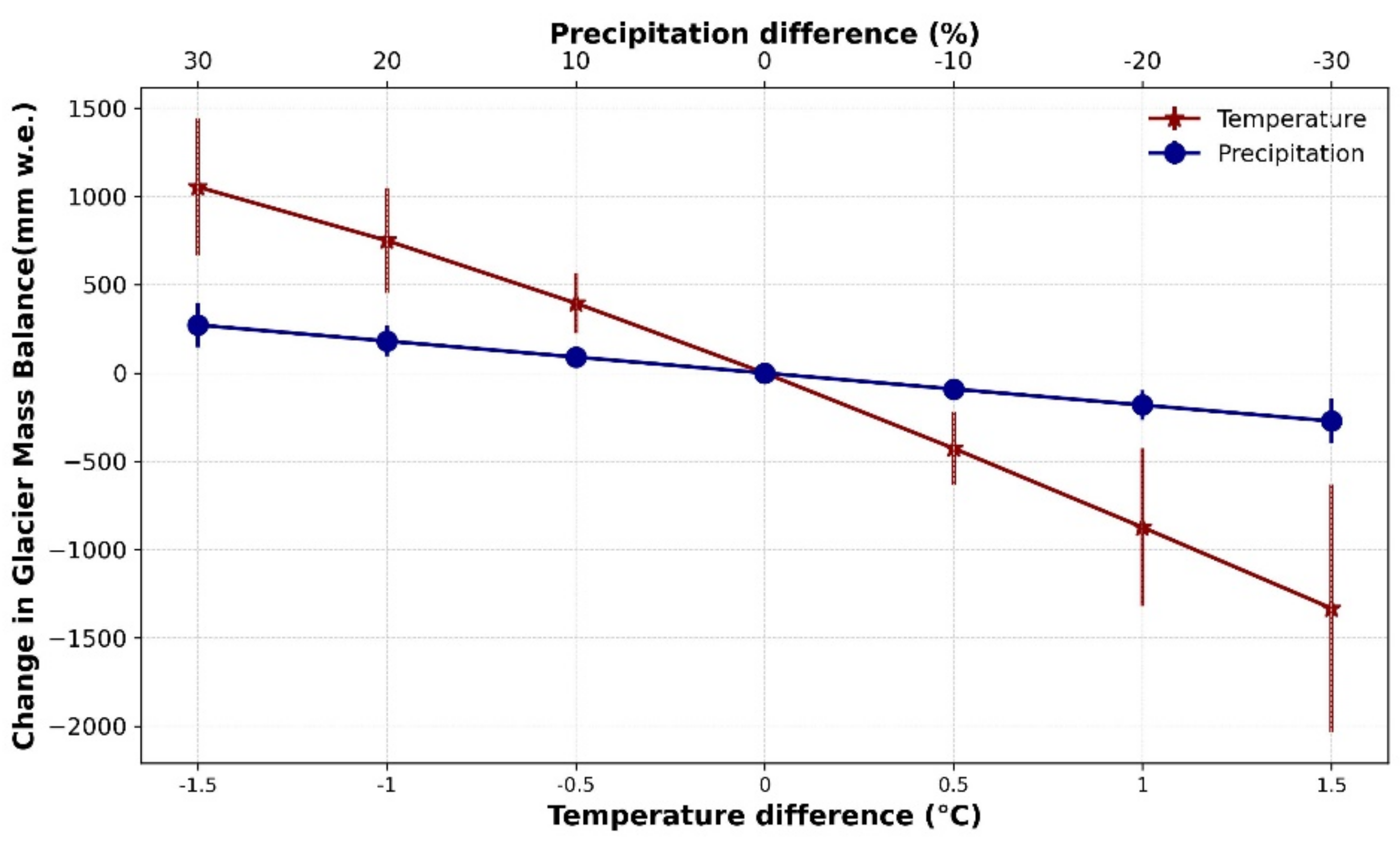
To investigate the SETP glacier sensitivity, our study investigated the sensitivity of all glaciers in the SETP using a series of sensitivity experiments conducted between 2000 and 2019. Specifically, we examined the changes in the SETP glaciers’ mass balance by adjusting a single parameter, either temperature or precipitation. Temperature adjustments ranged from −1.5 °C to 1.5 °C, with a unit of 0.5 °C, while precipitation adjustments ranged from −30% to 30%, with a unit of 10%. By manipulating these parameters, we assessed the corresponding changes in the glacier mass balance.
The findings revealed that the SETP glaciers exhibited a significantly higher sensitivity to temperature changes compared with the variations in precipitation (Figure 11). Notably, a temperature increase of 0.5 °C was found to have a pronounced impact on glacier loss. To compensate for a 0.5 °C temperature change in glacier mass balance, a substantial increase of over 30% in precipitation would be required.
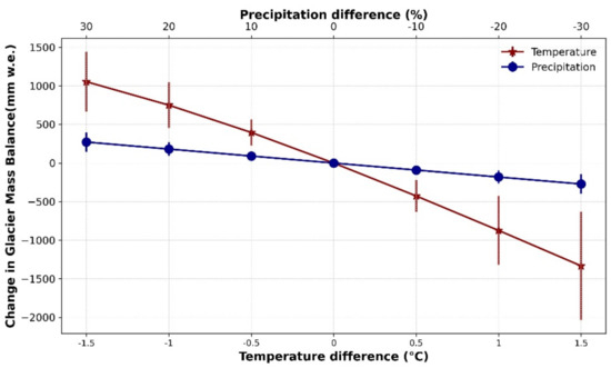
Figure 11.
Sensitivity analysis of SETP glaciers from 2000 to 2019, the temperature interval is 0.5 °C, changing between −1.5–1.5 °C, and the interval of precipitation is 10%, changing between −30% and 30%.
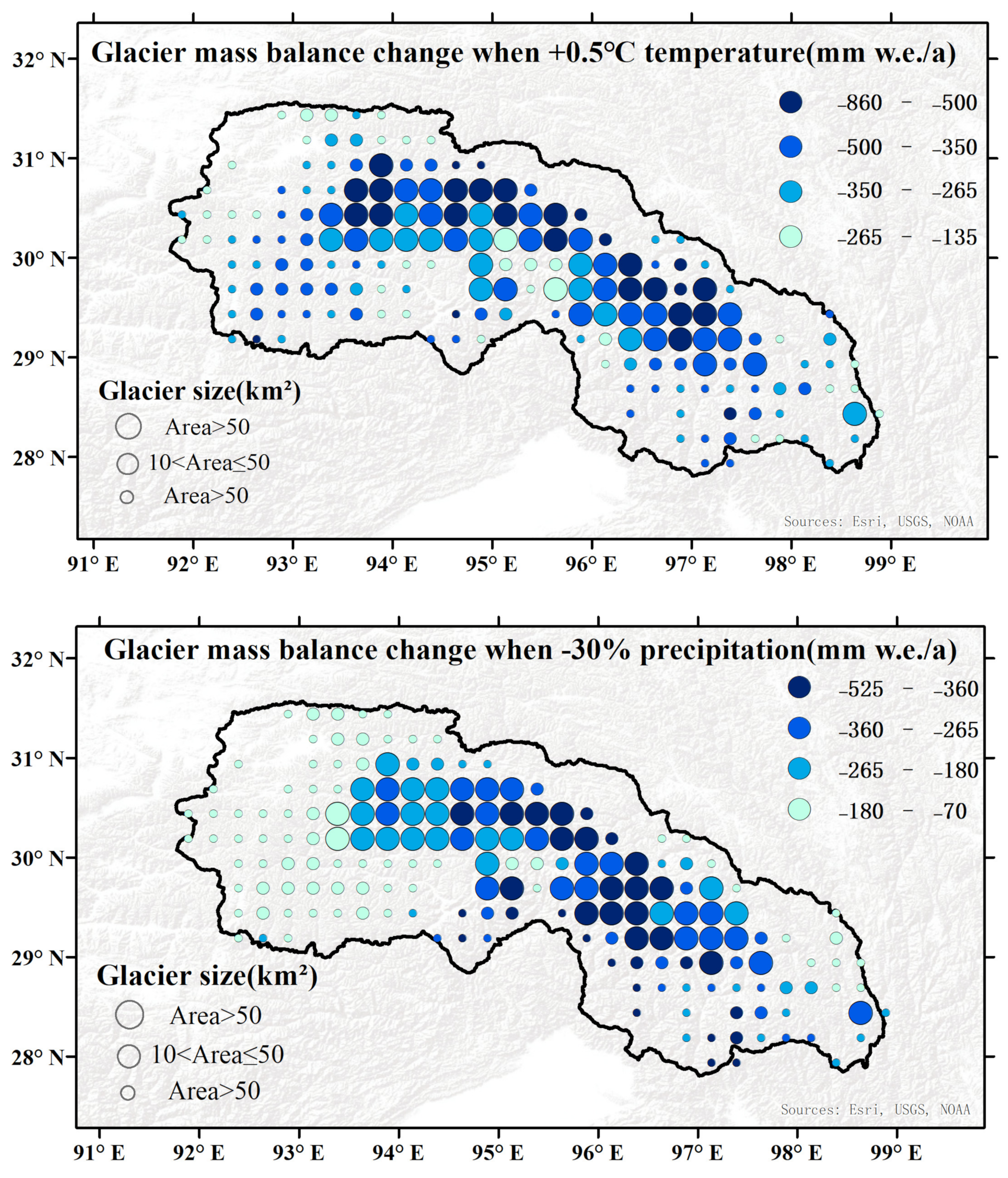
For further analysis, we discuss two scenarios where we set a 0.5 °C increase in temperature and a 30% decrease in the total precipitation and we investigated the spatial change in glaciers in the SETP (Figure 12). When we set a 0.5 °C increase in temperature, the glaciers in the upper SETP had severe mass loss, the lower SETP had relatively less mass loss, and the glaciers in the water vapor channel had the least mass loss. The lower SETP is closer to the Indian Ocean, and the summer monsoon brings a lot of precipitation to the lower SETP, especially the water vapor channel. When we set a 30% decrease in the total precipitation, the central and lower SETP were more sensitive to precipitation. As the lower part of the SETP serves as a central water vapor channel and features the lowest-altitude valley terrain, glaciers in this region primarily accumulate mass from the abundant precipitation brought by the Indian summer monsoon. Consequently, these glaciers exhibit greater stability in the face of precipitation changes compared to other regions within the SETP.

Figure 12.
Spatial change in glacier mass balance when setting single model parameters as +0.5 °C temperature or −30% precipitation.
5.2. Analysis of Climatic Considerations
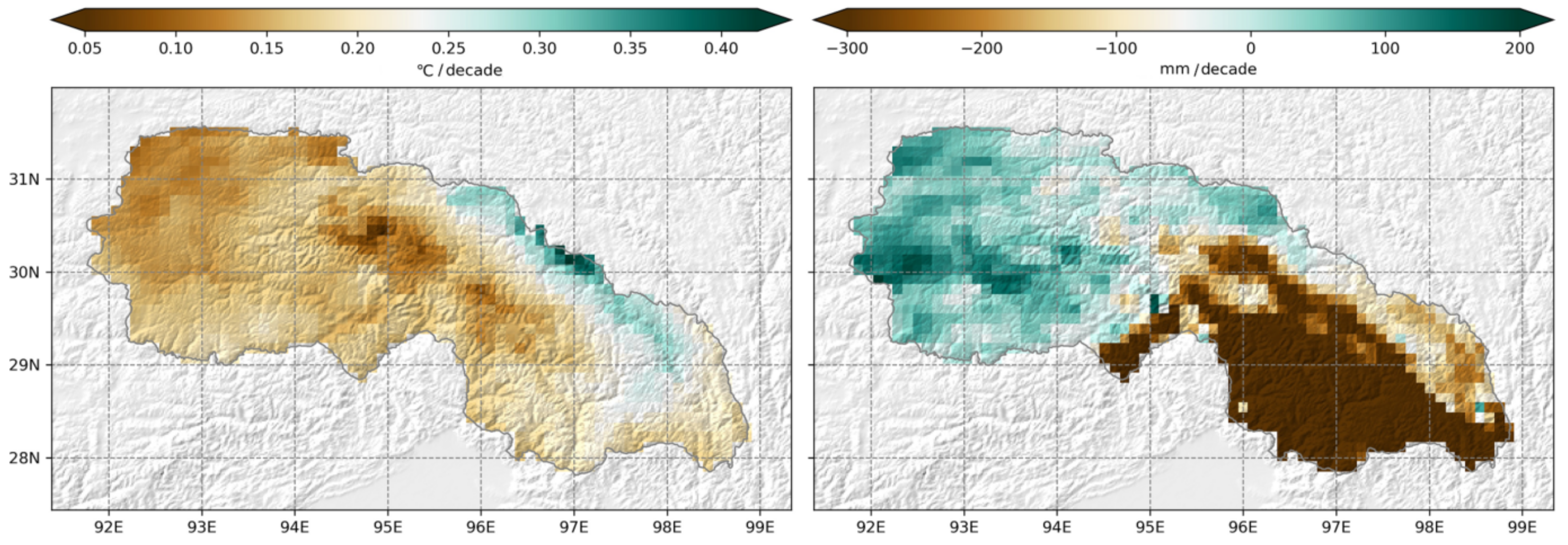
Regarding the model-driven HAR v2 data we used, we calculated the temperature rise rate of the SETP from 1980 to 2019, the unit was °C/decade. We found that during this period, the temperature in the entire SETP region showed a rising trend (Figure 13), though the rate showed obvious spatial heterogeneity. In the middle of the SETP, the area covered by glacier clusters was the area where the temperature rose the slowest in the entire SETP, mostly at 0.05~0.10 °C/decade. In the east and northeast of the SETP, the temperature shows a significant increase, exceeding 0.20 °C per decade and reaching a maximum of 0.42 °C per decade. Except for these two areas, the rest of the SETP presented a relatively stable temperature increase rate.

Figure 13.
The spatial distribution of the 10-year change rate of temperature and precipitation in the entire SETP region from 1980 to 2019. On the left, it shows 10-year change rate of temperature (°C/decade), and the figure on the right displays the 10-year change rate of precipitation (mm/decade).
In addition, we also analyzed the ten-year change rate of precipitation; we found that the overall precipitation change rate in the SETP did not show an obvious upward or downward trend, but it also had clear spatial heterogeneity. The precipitation in the southeastern part of the SETP showed an obvious decreasing trend, while the western part of the basin showed an increasing trend in precipitation. However, compared with the increasing precipitation, the decreasing trend in the southeastern part of the SETP was more obvious. We compared the temperature and precipitation change rate with seven national weather stations distributed in the SETP; we found that the temperature and precipitation change rate of the seven stations were in good agreement with the reanalysis data.
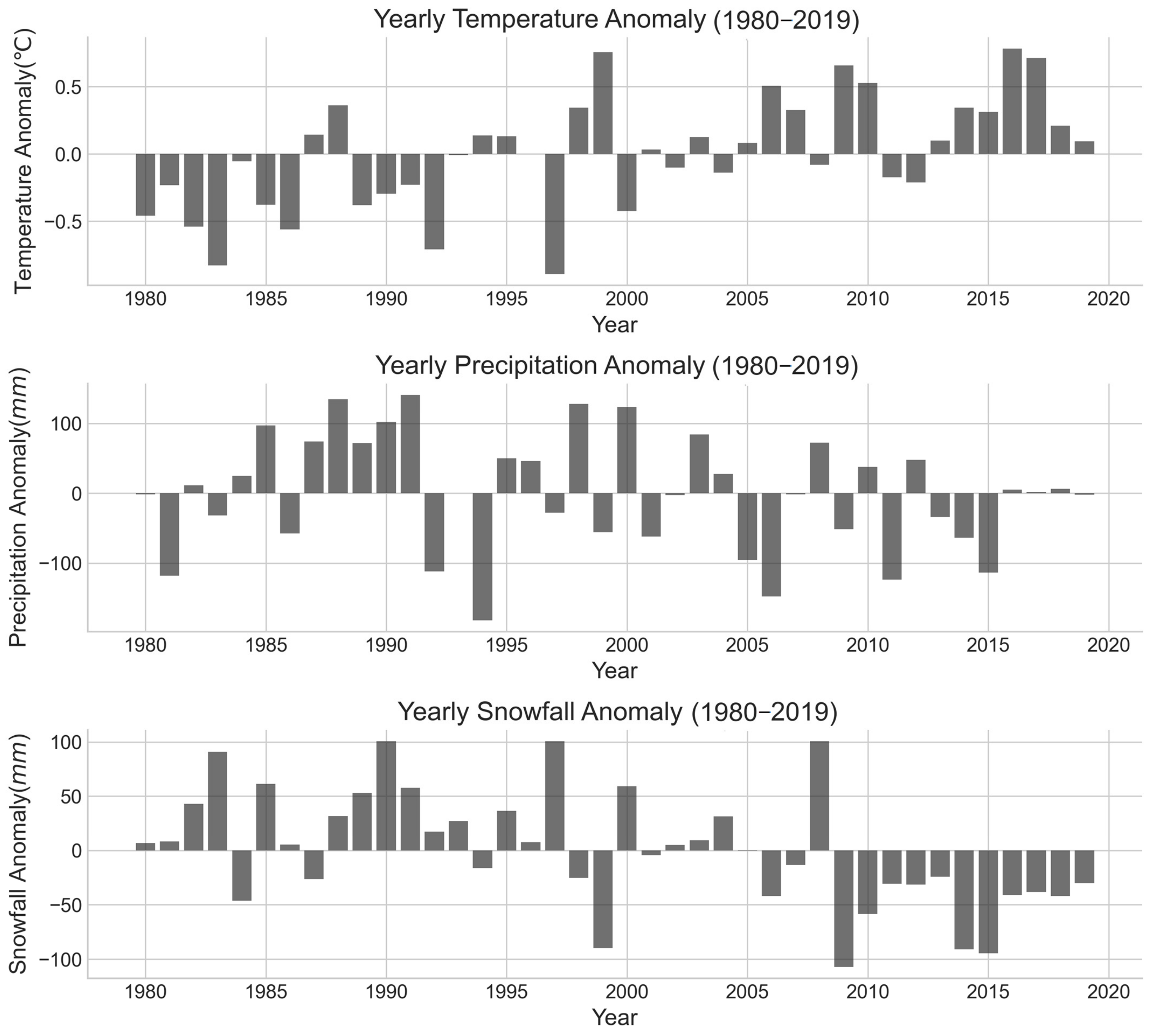
Regarding the spatial characteristics, we examined the rates of spatial change in temperature and precipitation. However, in terms of the time-series analysis for climate data, we needed to ascertain the overall trends in temperature and precipitation changes. Therefore, we calculated the abnormal values of temperature and precipitation by extracting the meteorological data grid points where the SETP glacier was located and obtained the time series of abnormal values of temperature and precipitation (Figure 14). Through the analysis, we found that the SETP temperature anomaly had obvious characteristics. In 1980–1999, the temperature anomaly was mostly negative, but in 2000–2019, the temperature anomaly was mostly positive. This was consistent with the mass balance characteristics calculated by us. The time series of the SETP precipitation anomalies showed no obvious regularity, but by observing the precipitation anomalies from 2000 to 2019, it was found that the overall trend of the SETP precipitation in this period showed a slight weakening.
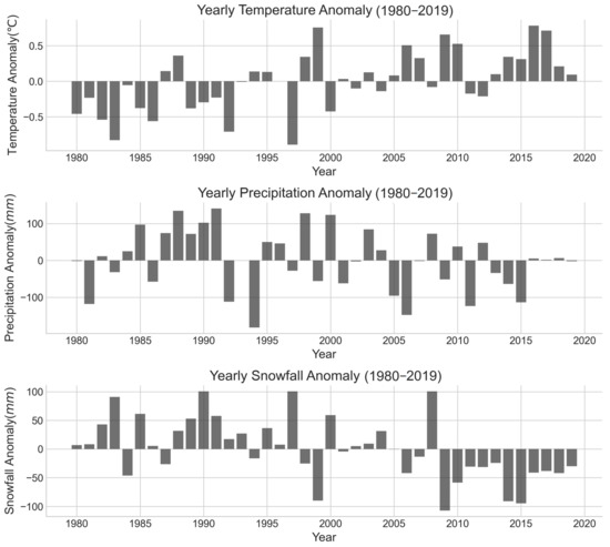
Figure 14.
The figure above shows temperature anomalies, precipitation anomalies, and snowfall anomalies in the SETP region from 1980 to 2019.
The rapid increase in temperature, coupled with a slight decline in precipitation, resulted in the glaciers of the SETP experiencing an accelerated rate of loss. When comparing the precipitation anomaly sequence with the snowfall anomaly time series, the latter displayed a discernible pattern and exhibited a certain correlation with temperature anomalies. Typically, the snowfall anomalies were positive when there was a negative temperature anomaly. When the temperature anomaly was positive, the snow anomaly was usually negative. This also confirmed that the anomalous rise in temperature made the phase transition from snowfall to rain occur in the SETP region. By studying these anomalies, we could identify the specific drivers of glacier melting and their relationship with climate change.
5.3. Weakening Summer-Monsoon-Induced Snowfall–Rainfall Transition
We analyzed the national weather station data distributed in the SETP from 1980–2019, the temperature of seven stations showed a consistent increase trend, while the precipitation showed a slight decrease in total. To further investigate the precipitation mechanisms, we chose the monsoon season (typically defined as June to September) as the yearly monsoon precipitation (Figure 15); we found four stations, namely, Bomi, Chayu, Linzhi, and Luolong, that showed a declining trend, while the other three stations, namely, Zuogong, Jiali, and Basu, showed a slightly increasing trend. The first four stations are closer to the Indian monsoon vapor channel, and thus, these decreases might have a relationship with the weaker magnitude of the Indian summer monsoon; the latter three stations might also be under the impact of a weaker summer monsoon, and their locations are relatively far away from the water vapor channel. In general, the overall declining trend in precipitation may have a relationship with weakened intensity of the Indian summer monsoon, this implies less cumulative precipitation during the monsoon season, leading the glaciers in the SETP to have lower incoming mass, and thus melting at a faster rate.
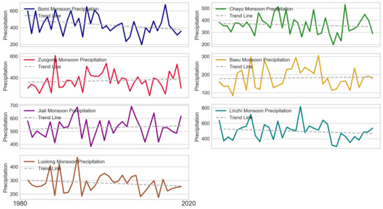
Figure 15.
Yearly monsoon season (June to September) precipitation of seven national weather stations in SETP from 1980 to 2019.
In our analysis of national weather station data from the SETP region spanning the years 1980 to 2019, we observed a consistent upward trend in temperature across seven stations, while the total precipitation exhibited a slight decrease. To further investigate the mechanisms behind these precipitation trends, we focused on the monsoon season (June to September). Our analysis (Figure 15) revealed varying trends at different stations: Bomi, Chayu, Linzhi, and Luolong exhibited declining precipitation, while Zuogong, Jiali, and Basu showed slight increases. The first four stations, which are closer to the Indian monsoon vapor channel, experienced declines that may be linked to the weakening strength of the Indian summer monsoon. Conversely, the latter three stations, which are situated further from the vapor channel, also seemed to be influenced by the weaker monsoon.
Overall, this declining trend in precipitation was likely associated with the delayed onset or weakened intensity of the Indian summer monsoon. This suggests reduced cumulative precipitation during the monsoon season, leading to diminished mass accumulation in the SETP glaciers.
To further investigate the alterations in snowfall and precipitation patterns and to substantiate the evidence supporting the weakened intensity of the summer monsoon, we analyzed the reanalysis data for grid points corresponding to the location of the SETP glaciers. This analysis was focused on the monsoon season.
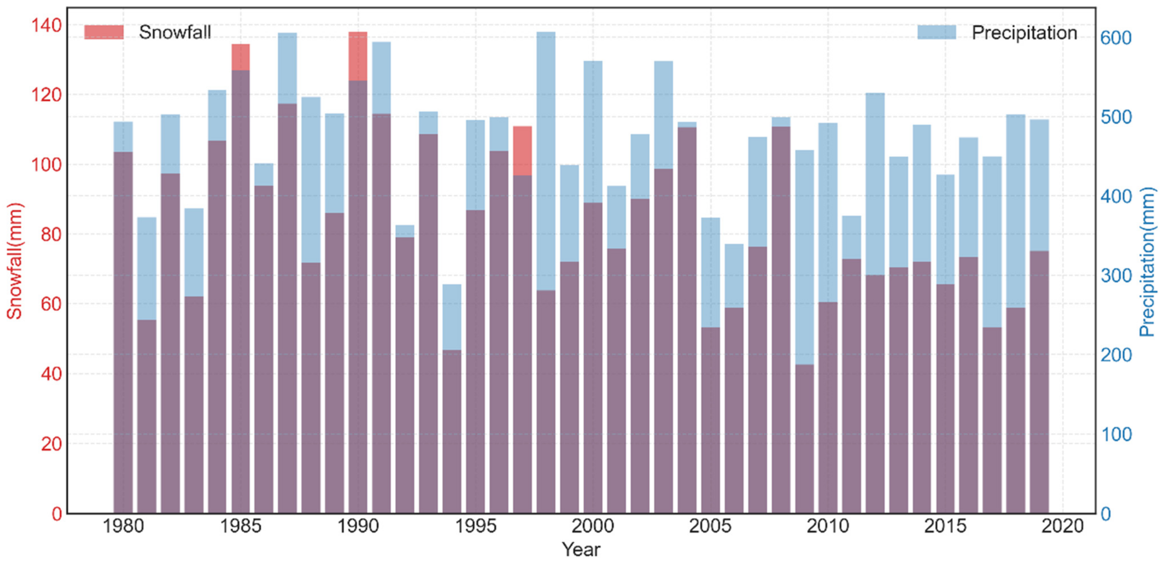
Our findings, which were based on the snowfall data, indicate that the SETP glaciers undertook their most significant melting during the monsoon season (June to September). However, due to specific terrain conditions and climatic factors, the SETP also experienced a certain degree of snowfall in the monsoon season. The analysis of data from 1980 to 2019 revealed a decreasing trend in snowfall during this period. Notably, after 2008, a significant decrease in snowfall was observed, which was concurrent with an increase in rainfall (Figure 16). This trend suggests that since the beginning of the 21st century, with notable temperature increases, the typical monsoon season snowfall in the SETP gradually transitioned into rainfall. Such a shift implicates the delayed onset or weakened intensity of the Indian summer monsoon in altering the precipitation and snowfall patterns. Consequently, this phase change in snowfall contributes to reduced mass replenishment of the glacier, leading to a continuous state of loss for the SETP glacier.
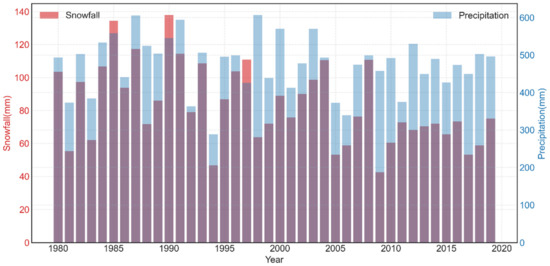
Figure 16.
Comparison of summer precipitation and snowfall in JJAS (June, July, August, September) in SETP from 1980 to 2019.
5.4. Uncertainty Analysis
The OGGM has multiple sources of uncertainty that require quantification. First, uncertainty arises from various external factors, as the model relies on datasets such as the RGI and DEMs for initial conditions, as well as atmospheric boundary conditions from the HAR v2 dataset and GCMs. These datasets convey their uncertainties to the model. Additionally, parameterizations are used to streamline and provide simplified approximations of physical processes that are not explicitly integrated into the model’s formulation [57]. However, the use of inappropriate parameterizations can introduce systematic errors into the model. Similarly, adopting uniform values for certain parameters across all glaciers (referred to as global parameters) and maintaining constant parameter values throughout the simulations are simplifications that can lead to inaccuracies. For example, in regions with a large amount of liquid precipitation, such as the SETP, the simplification of dynamic temperature thresholds for differentiating precipitation phases and the use of precipitation correction factors can potentially introduce errors in precipitation estimations and result in uncertain simulation outcomes. Third, the effects of debris cover also need to be considered. The presence of debris cover over glaciers has a significant influence on the glacier surface mass balance; however, existing glacier models have not yet accounted for these effects. One potential recommendation is to integrate a simple empirical model that establishes a relationship between debris thickness and temperature into the glacier evolution model. This coupling would enable the quantification of the influence of debris cover on glaciers.
Furthermore, there is potential for enhancing the method used to quantify the model uncertainty. While Bayesian inference and analysis of variance techniques have been applied to assess parameter uncertainty in hydrological models [58], aggregating and distinguishing uncertainties from individual to regional scales in glacier evolution models remains a considerable challenge. Therefore, future research should focus on examining the appropriateness and effectiveness of these methods for quantifying uncertainty in glacier evolution models.
6. Conclusions
In this study, the OGGM was employed to analyze the historical mass balance and future dynamics of glaciers in the SETP region. Due to the limited availability of measured glaciological data, regional geodetic datasets were used to calibrate and validate the model. The validation demonstrated the reliability of our simulations. Our analysis revealed that from 1980 to 2019, the average mass balance of the SETP glaciers was −0.50 ± 0.28 m w.e. a−1, and the magnitude of loss intensified after the 2000s, with a mass balance of −0.53 ± 0.27 m w.e. a−1 from 2000 to 2009 and −0.71 ± 0.15 m w.e. a−1 from 2010 to 2019. Furthermore, the spatial variations of the glacier mass balance were examined. Glaciers in the central region demonstrated comparatively smaller losses compared with those on the eastern and western sides. As we moved from the central region toward both sides, the mass loss became more severe.
In order to assess the future trends of glacier dynamics, we utilized four bias-corrected CMIP6 models. The ensemble forecasts indicate a significant decline in the glacier area, length, and volume. For the Mekong basin, the projected reductions were 78.01 ± 6.25% in the area, 86.59 ± 4.36% in the length, and 83.1 ± 6.83% in the volume. Similarly, for the Salween basin, the expected reductions were 95.03 ± 3.17% in the area, 95.50 ± 2.36% in the length, and 94.58 ± 2.60% in the volume. Lastly, for the Brahmaputra basin, the forecasted declines were 82.28 ± 5.07% in the area, 89.27 ± 4.46% in the length, and 87.32 ± 4.63% in the volume. Across the entire SETP, the glacier area, length, and volume are anticipated to decrease by 83.57 ± 4.91%, 90.05 ± 4.23%, and 88.04 ± 4.52%, respectively.
The future trend of glacier runoff will decline based on our projections, the glacier melt runoff will experience significant loss, while the future precipitation is projected to continuously increase in the future; therefore, the total runoff in the SETP will remain in a stable state.
Concerning the glacier melt runoff, as for the entire SETP, glacier melt runoff is forecasted to decrease by 62.63 ± 6.16% toward the end of this century, with the “peak water” point estimated to be in 2026 under SSP126 and SSP370, and in 2023 under SSP585. Within three basins in the SETP, the projected “peak water” point points are all anticipated to take place in the 2020–2030s.
The sensitivity analysis revealed that glaciers in the SETP region exhibited a pronounced sensitivity to changes in temperature in contrast with precipitation. Specifically, an increase in temperature of merely 0.5 °C required over 30% more precipitation to counterbalance the loss in glacier mass. Furthermore, a rapid rise in temperature within the SETP region was observed by the AWS and reanalysis data, and a slight decline in the precipitation was observed; this is evidence of the delayed onset or weakened magnitude of the summer monsoon. Moreover, the rising temperature and slight decline in precipitation caused a phase transition from snowfall to rainfall during the monsoon season.
Overall, these findings enhance our understanding of glacier change in the SETP and provide valuable insights for managing water resources and developing strategies to adapt to climate change. We suggest the need for more high-elevation observations combined with highly resolved atmospheric model simulations in the future.
Author Contributions
Conceptualization, K.W. and L.X.; investigation, Y.S., Y.D., Y.Y., J.Z. and J.W.; methodology, L.X., Y.Z. and M.M.A.; writing—original draft, L.X.; software, L.X. and S.L. (Shijie Li); writing—review and editing, S.L. (Shiyin Liu), Y.Z. and L.X. All authors have read and agreed to the published version of the manuscript.
Funding
This work was supported by the National Natural Science Foundation of China, grant no. 42361021; the National Key R&D Program of China, grant no. 2022YFF0711702-03; and the Natural Science Foundation of Yunnan, grant nos. 202301AT070417 and 202205AM070011.
Data Availability Statement
The High Asia Refined analysis version 2 (HAR v2) data used in this study are available from https://www.klima.tu-berlin.de/index.php?show=daten_har2 (accessed on 1 September 2023). The reference geodetic data used for calibration in this study are available from https://www.sedoo.fr/theia-publication-products/?uuid=c428c5b9-df8f-4f86-9b75-e04c778e29b9 (accessed on 23 September 2023).
Conflicts of Interest
The authors declare no conflicts of interest.
References
- Rounce, D.R.; Hock, R.; Maussion, F.; Hugonnet, R.; Kochtitzky, W.; Huss, M.; Berthier, E.; Brinkerhoff, D.; Compagno, L.; Copland, L.; et al. Global Glacier Change in the 21st Century: Every Increase in Temperature Matters. Science 2023, 379, 78–83. [Google Scholar] [CrossRef]
- Farinotti, D.; Huss, M.; Fürst, J.J.; Landmann, J.; Machguth, H.; Maussion, F.; Pandit, A. A Consensus Estimate for the Ice Thickness Distribution of All Glaciers on Earth. Nat. Geosci. 2019, 12, 168–173. [Google Scholar] [CrossRef]
- Hugonnet, R.; McNabb, R.; Berthier, E.; Menounos, B.; Nuth, C.; Girod, L.; Farinotti, D.; Huss, M.; Dussaillant, I.; Brun, F.; et al. Accelerated Global Glacier Mass Loss in the Early Twenty-First Century. Nature 2021, 592, 726–731. [Google Scholar] [CrossRef]
- Gardner, A.S.; Moholdt, G.; Cogley, J.G.; Wouters, B.; Arendt, A.A.; Wahr, J.; Berthier, E.; Hock, R.; Pfeffer, W.T.; Kaser, G.; et al. A Reconciled Estimate of Glacier Contributions to Sea Level Rise: 2003 to 2009. Science 2013, 340, 852–857. [Google Scholar] [CrossRef]
- Lutz, A.; Immerzeel, W.W.; Shrestha, A.; Bierkens, M.F.P. Consistent Increase in High Asia’s Runoff Due to Increasing Glacier Melt and Precipitation. Nat. Clim. Change 2014, 4, 587–592. [Google Scholar] [CrossRef]
- Immerzeel, W.; Lutz, A.; Andrade, M.; Bahl, A.; Biemans, H.; Bolch, T.; Hyde, S.; Brumby, S.; Davies, B.; Elmore, A.; et al. Importance and Vulnerability of the World’s Water Towers. Nature 2020, 577, 364–369. [Google Scholar] [CrossRef]
- Li, S.; Zhao, H.; Yu, W.; Yao, T.; Liu, S.; Wang, N.; Yang, W.; You, C.; Wang, W.; Wu, G.; et al. Glacier anomalies and relevant disaster risks on the Tibetan Plateau and surroundings. Chin. Sci. Bull. 2019, 64, 2770–2782. [Google Scholar] [CrossRef]
- Yao, T.; Bolch, T.; Chen, D.; Gao, J.; Immerzeel, W.; Piao, S.; Su, F.; Thompson, L.; Wada, Y.; Wang, L.; et al. The Imbalance of the Asian Water Tower. Nat. Rev. Earth Environ. 2022, 3, 618–632. [Google Scholar] [CrossRef]
- Yao, T.; Xue, Y.; Chen, D.; Chen, F.; Thompson, L.; Cui, P.; Koike, T.; Lau, W.; Lettenmaier, D.; Mosbrugger, V.; et al. Recent Third Pole’s Rapid Warming Accompanies Cryospheric Melt and Water Cycle Intensification and Interactions between Monsoon and Environment: Multidisciplinary Approach with Observations, Modeling, and Analysis. Bull. Am. Meteorol. Soc. 2019, 100, 423–444. [Google Scholar] [CrossRef]
- Zhang, Q.; Shen, Z.; Pokhrel, Y.; Farinotti, D.; Singh, V.P.; Xu, C.-Y.; Wu, W.; Wang, G. Oceanic Climate Changes Threaten the Sustainability of Asia’s Water Tower. Nature 2023, 615, 87–93. [Google Scholar] [CrossRef] [PubMed]
- Shean, D.E.; Bhushan, S.; Montesano, P.; Rounce, D.R.; Arendt, A.; Osmanoglu, B. A Systematic, Regional Assessment of High Mountain Asia Glacier Mass Balance. Front. Earth Sci. 2020, 7, 363. [Google Scholar]
- Brun, F.; Berthier, E.; Wagnon, P.; Kääb, A.; Treichler, D. A Spatially Resolved Estimate of High Mountain Asia Glacier Mass Balances from 2000 to 2016. Nat. Geosci. 2017, 10, 668–673. [Google Scholar] [CrossRef]
- Wang, Q.; Yi, S.; Sun, W. Continuous Estimates of Glacier Mass Balance in High Mountain Asia Based on ICESat-1,2 and GRACE/GRACE Follow-On Data. Geophys. Res. Lett. 2021, 48, e2020GL090954. [Google Scholar] [CrossRef]
- Fan, Y.; Ke, C.-Q.; Zhou, X.; Shen, X.; Yu, X.; Lhakpa, D. Glacier Mass-Balance Estimates over High Mountain Asia from 2000 to 2021 Based on ICESat-2 and NASADEM. J. Glaciol. 2023, 69, 500–512. [Google Scholar] [CrossRef]
- Yao, T.; Thompson, L.; Yang, W.; Yu, W.; Gao, Y.; Guo, X.; Yang, X.; Duan, K.; Zhao, H.; Xu, B.; et al. Different Glacier Status with Atmospheric Circulations in Tibetan Plateau and Surroundings. Nat. Clim. Change 2012, 2, 663–667. [Google Scholar] [CrossRef]
- Wu, K.; Liu, S.; Jiang, Z.; Xu, J.; Wei, J. Glacier Mass Balance over the Central Nyainqentanglha Range during Recent Decades Derived from Remote-Sensing Data. J. Glaciol. 2019, 65, 422–439. [Google Scholar] [CrossRef]
- Gardelle, J.; Berthier, E.; Arnaud, Y.; Kääb, A. Region-Wide Glacier Mass Balances over the Pamir-Karakoram-Himalaya during 1999–2011. Cryosphere 2013, 7, 1263–1286. [Google Scholar] [CrossRef]
- Xie, F.; Liu, S.; Gao, Y.; Zhu, Y.; Bolch, T.; Kääb, A.; Duan, S.; Miao, W.; Kang, J.; Zhang, Y.; et al. Interdecadal Glacier Inventories in the Karakoram since the 1990s. Earth Syst. Sci. Data 2023, 15, 847–867. [Google Scholar] [CrossRef]
- Mölg, T.; Maussion, F.; Scherer, D. Mid-Latitude Westerlies as a Driver of Glacier Variability in Monsoonal High Asia. Nat. Clim. Change 2014, 4, 68–73. [Google Scholar] [CrossRef]
- Zhu, M.; Yao, T.; Yang, W.; Xu, B.; Wu, G.; Wang, X. Differences in Mass Balance Behavior for Three Glaciers from Different Climatic Regions on the Tibetan Plateau. Clim. Dyn. 2018, 50, 3457–3484. [Google Scholar] [CrossRef]
- Mölg, T.; Maussion, F.; Yang, W.; Scherer, D. The Footprint of Asian Monsoon Dynamics in the Mass and Energy Balance of a Tibetan Glacier. Cryosphere Discuss. 2012, 6, 1445–1461. [Google Scholar] [CrossRef]
- Zhao, P.; Wang, B.; Zhou, X. Boreal Summer Continental Monsoon Rainfall and Hydroclimate Anomalies Associated with the Asia-Pacific Oscillation. Clim. Dyn. 2012, 39, 1197–1207. [Google Scholar] [CrossRef]
- Yang, W.; Guo, X.; Yao, T.; Zhu, M.; Wang, Y. Recent Accelerating Mass Loss of Southeast Tibetan Glaciers and the Relationship with Changes in Macroscale Atmospheric Circulations. Clim. Dyn. 2016, 47, 805–815. [Google Scholar] [CrossRef]
- Zhao, F.; Long, D.; Li, X.; Huang, Q.; Han, P. Rapid Glacier Mass Loss in the Southeastern Tibetan Plateau since the Year 2000 from Satellite Observations. Remote Sens. Environ. 2022, 270, 112853. [Google Scholar] [CrossRef]
- Zemp, M.; Huss, M.; Thibert, E.; Eckert, N.; McNabb, R.; Huber, J.; Barandun, M.; Machguth, H.; Nussbaumer, S.U.; Gärtner-Roer, I.; et al. Global Glacier Mass Changes and Their Contributions to Sea-Level Rise from 1961 to 2016. Nature 2019, 568, 382–386. [Google Scholar] [CrossRef] [PubMed]
- Luo, L.; Ke, C.-Q.; Fan, Y.; Wang, Z. Accelerated Glacier Mass Loss in the Southeastern Tibetan Plateau since the 1970s. Adv. Clim. Change Res. 2023, 14, 372–386. [Google Scholar] [CrossRef]
- Yang, W.; Yao, T.; Guo, X.; Zhu, M.; Li, S.; Kattel, D.B. Mass Balance of a Maritime Glacier on the Southeast Tibetan Plateau and Its Climatic Sensitivity. J. Geophys. Res. Atmos. 2013, 118, 9579–9594. [Google Scholar] [CrossRef]
- Ding, B.; Yang, K.; Yang, W.; Xiaobo, H.; Chen, Y.; Zhu, L.; Guo, X.; Wang, L.; Wu, H.; Yao, T. Development of a Water and Enthalpy Budget-Based Glacier Mass Balance Model (WEB-GM) and Its Preliminary Validation. Water Resour. Res. 2017, 53, 3146–3178. [Google Scholar] [CrossRef]
- Huss, M.; Hock, R. Global-Scale Hydrological Response to Future Glacier Mass Loss. Nat. Clim. Change 2018, 8, 135–140. [Google Scholar] [CrossRef]
- Hock, R. Temperature Index Melt Modelling in Mountain Areas. J. Hydrol. 2003, 282, 104–115. [Google Scholar] [CrossRef]
- Hock, R.; Bliss, A.; Marzeion, B.; Giesen, R.H.; Hirabayashi, Y.; Huss, M.; Radić, V.; Slangen, A.B.A. GlacierMIP—A Model Intercomparison of Global-Scale Glacier Mass-Balance Models and Projections. J. Glaciol. 2019, 65, 453–467. [Google Scholar] [CrossRef]
- Maussion, F.; Butenko, A.; Champollion, N.; Dusch, M.; Eis, J.; Fourteau, K.; Gregor, P.; Jarosch, A.H.; Landmann, J.; Oesterle, F.; et al. The Open Global Glacier Model (OGGM) v1.1. Geosci. Model Dev. 2019, 12, 909–931. [Google Scholar] [CrossRef]
- Zhao, H.; Su, B.; Lei, H.; Zhang, T.; Xiao, C. A New Projection for Glacier Mass and Runoff Changes over High Mountain Asia. Sci. Bull. 2023, 68, 43–47. [Google Scholar] [CrossRef]
- Mannan Afzal, M.; Wang, X.; Sun, L.; Jiang, T.; Kong, Q.; Luo, Y. Hydrological and Dynamical Response of Glaciers to Climate Change Based on Their Dimensions in the Hunza Basin, Karakoram. J. Hydrol. 2023, 617, 128948. [Google Scholar] [CrossRef]
- Tang, S.; Vlug, A.; Piao, S.; Li, F.; Wang, T.; Krinner, G.; Li, L.Z.X.; Wang, X.; Wu, G.; Li, Y.; et al. Regional and Tele-Connected Impacts of the Tibetan Plateau Surface Darkening. Nat. Commun. 2023, 14, 32. [Google Scholar] [CrossRef] [PubMed]
- Schuster, L.; Rounce, D. Fabien Maussion Glacier Projections Sensitivity to Temperature-Index Model Choices and Calibration Strategies. Ann. Glaciol. 2023, 1–16. [Google Scholar] [CrossRef]
- Eis, J.; Maussion, F.; Marzeion, B. Initialization of a Global Glacier Model Based on Present-Day Glacier Geometry and Past Climate Information: An Ensemble Approach. Cryosphere 2019, 13, 3317–3335. [Google Scholar] [CrossRef]
- Eis, J.; van der Laan, L.; Maussion, F.; Marzeion, B. Reconstruction of Past Glacier Changes with an Ice-Flow Glacier Model: Proof of Concept and Validation. Front. Earth Sci. 2021, 9, 595755. [Google Scholar] [CrossRef]
- Pfeffer, W.T.; Arendt, A.A.; Bliss, A.; Bolch, T.; Cogley, J.G.; Gardner, A.S.; Hagen, J.-O.; Hock, R.; Kaser, G.; Kienholz, C.; et al. The Randolph Glacier Inventory: A Globally Complete Inventory of Glaciers. J. Glaciol. 2014, 60, 537–552. [Google Scholar] [CrossRef]
- Shi, Y.; Liu, S. Estimation on the Response of Glaciers in China to the Global Warming in the 21st Century. Chin. Sci. Bull. 2000, 45, 668–672. [Google Scholar] [CrossRef]
- Jouberton, A.; Shaw, T.E.; Miles, E.; McCarthy, M.; Fugger, S.; Ren, S.; Dehecq, A.; Yang, W.; Pellicciotti, F. Warming-Induced Monsoon Precipitation Phase Change Intensifies Glacier Mass Loss in the Southeastern Tibetan Plateau. Proc. Natl. Acad. Sci. USA 2022, 119, e2109796119. [Google Scholar] [CrossRef]
- Zheng, G.; Mergili, M.; Emmer, A.; Allen, S.; Bao, A.; Guo, H.; Stoffel, M. The 2020 Glacial Lake Outburst Flood at Jinwuco, Tibet: Causes, Impacts, and Implications for Hazard and Risk Assessment. Cryosphere 2021, 15, 3159–3180. [Google Scholar] [CrossRef]
- Wang, X.; Tolksdorf, V.; Otto, M.; Scherer, D. WRF-based Dynamical Downscaling of ERA5 Reanalysis Data for High Mountain Asia: Towards a New Version of the High Asia Refined Analysis. Int. J. Climatol. 2020, 41, 743–762. [Google Scholar] [CrossRef]
- Huintjes, E.; Loibl, D.; Lehmkuhl, F.; Schneider, C. A Modelling Approach to Reconstruct Little Ice Age Climate from Remote-Sensing Glacier Observations in Southeastern Tibet. Ann. Glaciol. 2016, 57, 359–370. [Google Scholar] [CrossRef]
- Khadka, A.; Wagnon, P.; Brun, F.; Shrestha, D.; Lejeune, Y.; Arnaud, Y. Evaluation of ERA5-Land and HARv2 Reanalysis Data at High Elevation in the Upper Dudh Koshi Basin (Everest Region, Nepal). J. Appl. Meteorol. Climatol. 2022, 61, 931–954. [Google Scholar] [CrossRef]
- Eyring, V.; Bony, S.; Meehl, G.A.; Senior, C.A.; Stevens, B.; Stouffer, R.J.; Taylor, K.E. Overview of the Coupled Model Intercomparison Project Phase 6 (CMIP6) Experimental Design and Organization. Geosci. Model Dev. 2016, 9, 1937–1958. [Google Scholar] [CrossRef]
- Zhang, W.; Liu, L.; Lun, Y.; Cheng, L.; Li, X.; Xu, Z. Projections of Future Precipitation and Air Temperature over the Tibetan Plateau Based on CMIP6 Multi-model Ensembles. Int. J. Climatol. 2022, 42, 9788–9822. [Google Scholar] [CrossRef]
- Tokarska, K.; Stolpe, M.; Sippel, S.; Fischer, E.; Smith, C.; Lehner, F.; Knutti, R. Past Warming Trend Constrains Future Warming in CMIP6 Models. Sci. Adv. 2020, 6, eaaz9549. [Google Scholar] [CrossRef]
- Cook, B.; Mankin, J.; Marvel, K.; Williams, A.; Smerdon, J.; Anchukaitis, K. Twenty-First Century Drought Projections in the CMIP6 Forcing Scenarios. Earth’s Future 2020, 8, e2019EF001461. [Google Scholar] [CrossRef]
- Chen, R.; Duan, K.; Shang, W.; Shi, P.; Meng, Y.; Zhang, Z. Increase in Seasonal Precipitation over the Tibetan Plateau in the 21st Century Projected Using CMIP6 Models. Atmos. Res. 2022, 277, 106306. [Google Scholar] [CrossRef]
- Crippen, R.; Buckley, S.; Agram, P.; Belz, E.; Gurrola, E.; Hensley, S.; Kobrick, M.; Lavalle, M.; Martin, J.; Neumann, M.; et al. Nasadem Global Elevation Model: Methods And Progress. ISPRS—Int. Arch. Photogramm. Remote Sens. Spat. Inf. Sci. 2016, 41, 125–128. [Google Scholar] [CrossRef]
- OGGM/Oggm: V1.6.1. Available online: https://doi.org/10.5281/zenodo.8287580 (accessed on 1 September 2023).
- Marzeion, B.; Jarosch, A.H.; Hofer, M. Past and Future Sea-Level Change from the Surface Mass Balance of Glaciers. Cryosphere 2012, 6, 1295–1322. [Google Scholar] [CrossRef]
- Huss, M.; Hock, R. A New Model for Global Glacier Change and Sea-Level Rise. Front. Earth Sci. 2015, 3, 54. [Google Scholar] [CrossRef]
- Wu, K.; Liu, S.; Jiang, Z.; Xu, J.; Wei, J.; Guo, W. Recent Glacier Mass Balance and Area Changes in the Kangri Karpo Mountains from DEMs and Glacier Inventories. Cryosphere 2018, 12, 103–121. [Google Scholar] [CrossRef]
- Sakai, A.; Fujita, K. Contrasting Glacier Responses to Recent Climate Change in High-Mountain Asia. Sci. Rep. 2017, 7, 13717. [Google Scholar] [CrossRef]
- Recinos, B.; Maussion, F.; Rothenpieler, T.; Marzeion, B. Impact of Frontal Ablation on the Ice Thickness Estimation of Marine-Terminating Glaciers in Alaska. Cryosphere 2019, 13, 2657–2672. [Google Scholar] [CrossRef]
- Rounce, D.R.; Hock, R.; Shean, D.E. Glacier Mass Change in High Mountain Asia through 2100 Using the Open-Source Python Glacier Evolution Model (PyGEM). Front. Earth Sci. 2020, 7, 331. [Google Scholar] [CrossRef]
Disclaimer/Publisher’s Note: The statements, opinions and data contained in all publications are solely those of the individual author(s) and contributor(s) and not of MDPI and/or the editor(s). MDPI and/or the editor(s) disclaim responsibility for any injury to people or property resulting from any ideas, methods, instructions or products referred to in the content. |
© 2024 by the authors. Licensee MDPI, Basel, Switzerland. This article is an open access article distributed under the terms and conditions of the Creative Commons Attribution (CC BY) license (https://creativecommons.org/licenses/by/4.0/).

