Article

Radar Reconnaissance Pulse-Splitting Modeling and Detection Method

1
School of Electronic Engineering, Xidian University, Xi’an 710071, China
2
Unit 93209 of PLA, Beijing 100085, China
*
Author to whom correspondence should be addressed.
Remote Sens. 2024, 16(3), 521; https://doi.org/10.3390/rs16030521
Submission received: 4 December 2023 / Revised: 24 January 2024 / Accepted: 25 January 2024 / Published: 29 January 2024
(This article belongs to the Topic Radar Signal and Data Processing with Applications)

Abstract

:
When radar receivers adopt digital channelization, it is prone to generating a cross-channel split signal, the rabbit ear effect, and a transition band repeated signal, leading to errors in radar signal sorting or identification. The pulse-splitting model and detection method proposed in this paper can model split pulses and identify them in radar pulse streams, facilitating the merging of split pulses to enhance sorting and identification performance. Firstly, the mechanism of splitting pulse generation is deeply analyzed, and the splitting site theory is proposed. Then, the split pulse signal model and the split pulse number statistical model based on geometric distribution are constructed, which are used to guide the construction of simulation data of split pulse flow with different characteristics. Furthermore, a time-domain convergence degree (TCD) index is proposed to characterize the pulse split phenomenon. At the same time, in order to avoid a large number of threshold searching problems in pulse-splitting detection, an empirical formula for the pulse-splitting detection threshold based on the TCD is given to quickly determine whether there is a pulse train split problem. The selected measured radar pulse stream is verified to follow a geometric distribution at a significance level of 0.05. The proposed method achieved a detection accuracy of at least 99.55% on the simulation dataset and at least 95.68% on the experimental dataset, validating the rationality of pulse-splitting modeling and the effectiveness of the detection method.

1. Introduction

The reliable and accurate detection of non-cooperative radar pulses is one of the key tasks of radar reconnaissance. The detection results are crucial for estimating radar frequency, pulse width (PW), and other parameters. The quality of parameter estimation directly impacts subsequent tasks such as sorting recognition and jamming decision making [1,2].
For the detection of radar pulse signals in reconnaissance signals, the basic principle is to utilize the differences in statistical characteristics between random noise and signals in various transform domains. The most classic algorithm is the time-domain energy detection method, whose performance is significantly affected by noise [3]. Xi Yimin [4] and Zou Simin [5] achieved pulse detection under low signal-to-noise ratio (SNR) conditions by computing the delayed autocorrelation of the received signal. Li Cheng [2] utilizes the Difference of Boxes (DOB) filter for pulse edge detection, and its detection performance surpasses that of an energy detection method [3]. On the basis of Li Cheng [2], Xinqun Liu [6] utilizes the fine-tuned Short-Time Fourier Transform (STFT) to refine the rough pulse edge, and then the Constant False Alarm Rate (CFAR) method is used to implement adaptive threshold detection in the frequency domain, which is better than the DOB pulse detection algorithm [2] and the traditional energy detection method [3]. Wenmao Luo [7] utilizes the disparity in state variables between two generalized time-scale transformed Duffing oscillators to detect pulses, thereby addressing the issue of weak pulse signal detection. Existing radar pulse detection algorithms [2,3,4,5,6,7] focus on detecting individual pulses, but prior to this paper, no one has studied the detection of split radar pulses.
There are several factors that affect pulse detection performance, and CAO Chunyan [8] has conducted a comprehensive analysis focusing on SNR, pulse overlap, and processing channels. However, the complex and variable modern electromagnetic environment results in a significant difference in correlation power, various modulation forms, and a serious time-domain overlap in the receiver [9]. The received pulse signal is prone to splitting due to multipath effects, equipment impedance mismatch, and colored noise [10]. The use of ultra-wideband radar [11] with high-resolution detection capability will cause a serious split phenomenon in both the time-domain and frequency-domain detection methods based on digital channalization, which is not conducive to reliable detection and analysis of ultra-wideband radar. In particular, Guangliang Zou [12], Ying Liu [13] and Haiqing Jiang [14] point out that wideband pulse amplitude (PA) is susceptible to noise, fluctuates greatly in its interior, and the intra-pulse data segment is prone to be lower than the minimum detection sensitivity, thus causing pulse splitting.
In view of the pulse split phenomenon, Guangliang Zou [12] uses the correlation of adjacent pulse description words (PDW) in the time-frequency domain and the consistency of intra-pulse modulation types to solve the merging of split PDWs. Ying Liu [13] considers the misjudgment of intra-pulse modulation type caused by insufficient linearity when there are fewer intra-pulse sample points. It also removes the constraint condition of the intra-pulse modulation type mentioned in reference [12]. Ying Liu [13] designs the merging conditions for split pulses under different modulation types. The corresponding parameters after merging are obtained by averaging the PA and frequency-modulated slope of the split pulses that satisfy the merging condition. Then, the corresponding expression for the combination of multiple split pulses in the time-frequency domain parameter is constructed. Different from Ying Liu [13], Haiqing Jiang [14] considers the actual measurement error and introduces the error coefficient into the LFM parameters and frequency domain merging conditions. Liming Tang [15] proposes a serial combination judgment method that judges the signal type, the time of arrival (TOA) difference of adjacent pulses, the difference of pulse slope, and the center frequency in turn. When the combination condition is met step by step, the pulse combination process is carried out with the weight of the split PW. Chao Wang [16] provides a theoretical basis for constructing the split pulse signal model through mathematical modeling of the split linear frequency modulation signal.
The pulse-splitting model proposed in this paper analyzes the mechanisms behind three pulse-splitting phenomena: the cross-channel split signal, the rabbit ear effect, and the transition band repeated signal. Furthermore, this paper establishes correspondences between the three pulse-splitting phenomena and the temporal relationships among the split pulses: the temporal relationship of cross-channel split signal pulses is overlapping, the temporal relationship of rabbit ear effect split pulses is independent, and the temporal relationship of transition band repeated signal split pulses is inclusive. Subsequently, a split pulse signal model covering the above three pulse-splitting phenomena is proposed. Finally, this paper also discovers and verifies that the statistical distribution of split pulse counts follows a geometric distribution. Wu Zhenyu [17] and Gui Youlin [18] conducted a mechanistic study on the three scenarios of pulse splitting described above. Guangliang Zou [12], Ying Liu [13], Haiqing Jiang [14], and Liming Tang [15] outlined the merging conditions and methods of split pulses. However, none of them, including Guangliang Zou [12], Ying Liu [13], Haiqing Jiang [14], Liming Tang [15], Wu Zhenyu [17], and Gui Youlin [18], has mathematically modeled the phenomenon of pulse splitting. Wang Chao [16]’s proposed pulse-splitting model only addresses independently timed split pulses and does not consider other splitting scenarios. Additionally, none of these researchers have investigated the statistical regularity of split pulse numbers.
The advantages and disadvantages of existing radar pulse-splitting methods are shown in Table 1. Aiming to address the lack of research on the pulse-splitting model and detection method, the main contributions of the proposed pulse-splitting modeling and detection method are as follows:
  • The split-site theory is proposed to describe the mechanism of split pulses in different ways. Then, based on the split pulse law of the experimental data, the split pulse signal model and the statistical model of the number of split pulses using the geometric distribution are constructed, respectively. Subsequently, simulation data of split pulses with various characteristics are generated using the proposed model.
  • A convergence degree in the time domain is proposed to represent pulse splitting. Additionally, based on the TCD, an empirical formula is provided for the threshold of pulse-splitting detection. This formula helps to avoid the low detection efficiency that can be caused by a large number of threshold searches in pulse splitting detection, enabling the reliable assessment of pulse splitting in a radar pulse stream.
This paper presents the concept of split pulse fusion processing and signal parameter estimation. It can improve the sorting and identification performance, supports the efficient and reliable implementation of radar reconnaissance systems, and has significant engineering application value.

2. Pulse-Splitting Model

When receiving the non-cooperative radar pulses, the pulse-splitting phenomenon will be caused by the environment and the detection equipment, which makes the reconnaissance process difficult. By analyzing the split law of the experimental data, the generation mechanism of the split pulse is expounded according to the problems brought by digital channelization, and the split site theory is proposed to describe the split pulse of different split modes. Then, a statistical model is constructed for the number of split pulses based on the geometric distribution. The split site theory is then incorporated to guide the construction of split pulse flows with different characteristics.

2.1. Modeling Pulse-Splitting Phenomena

2.1.1. Split Pulse Generation Mechanism

In this paper, the phenomenon of pulse splitting caused by the receiver device is primarily considered. The digital channelization receiver device divides the receiver bandwidth into multiple subchannels and outputs signals of different frequencies through a set of filters that can cover the entire frequency band. Digital channelization has many advantages, such as the ability to handle wideband signals and signals arriving at different frequencies simultaneously. However, there are still problems such as the cross-channel signal split phenomenon, the rabbit ear effect, and the repetition of signals in the transition band, which are collectively referred to as the pulse split phenomenon [17,18]. In the following, the split-site theory is proposed, and the mechanism of the above pulse split phenomenon is described, respectively.
  • Split Site Theory
As shown in Figure 1, the original pulse is located on the upper time axis, while the split pulse generated by the original pulse is located on the lower time axis. The split sites 1 to 10 represent the leading edge and the trailing edge of the split pulse, respectively, for the original pulse; the number of split pulses is 5. The relationship between the number of split sites and the number of split pulses of a single original pulse can be determined as follows:
M = 2 · N
According to the experimental data of split pulses, the following provisions are made:
  • The split sites in a complete pulse are not allowed to be reused; that is, a split site can only be used as the leading edge or trailing edge of a split pulse.
  • The current split site can only generate a split pulse with the next split site.
  • Split pulses are only allowed to be generated in a single complete pulse.
  • The first split site must be located at the leading edge of the complete pulse, and the last split site must be located at the trailing edge of the complete pulse.
  • All split sites within a complete pulse must be used.
Let any adjacent split pulse split by the same original pulse with earlier arrival time be the n number subpulse and the later one be the n + 1 number subpulse. The n number subpulse arrival time front is T O A n , the front site is a, the back edge of the arrival time is T O E n , and the back edge site is a + x . The n + 1 subpulse arrival time front is T O A n + 1 , the front site is b, the arrival time back edge is T O E n + 1 , and the back edge site is b + y , a , b , x , y N .
  • Cross-channel splitting signal
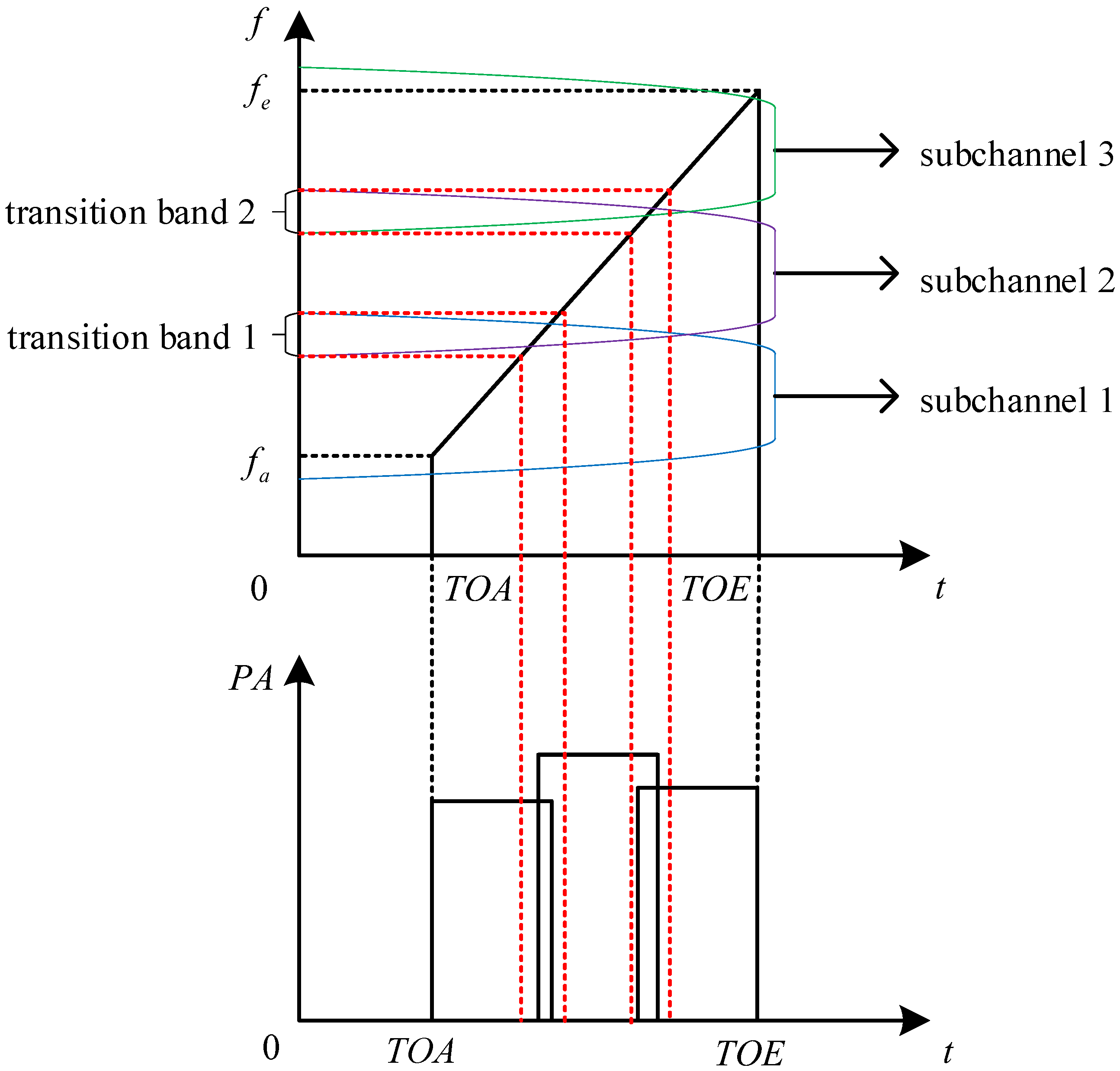
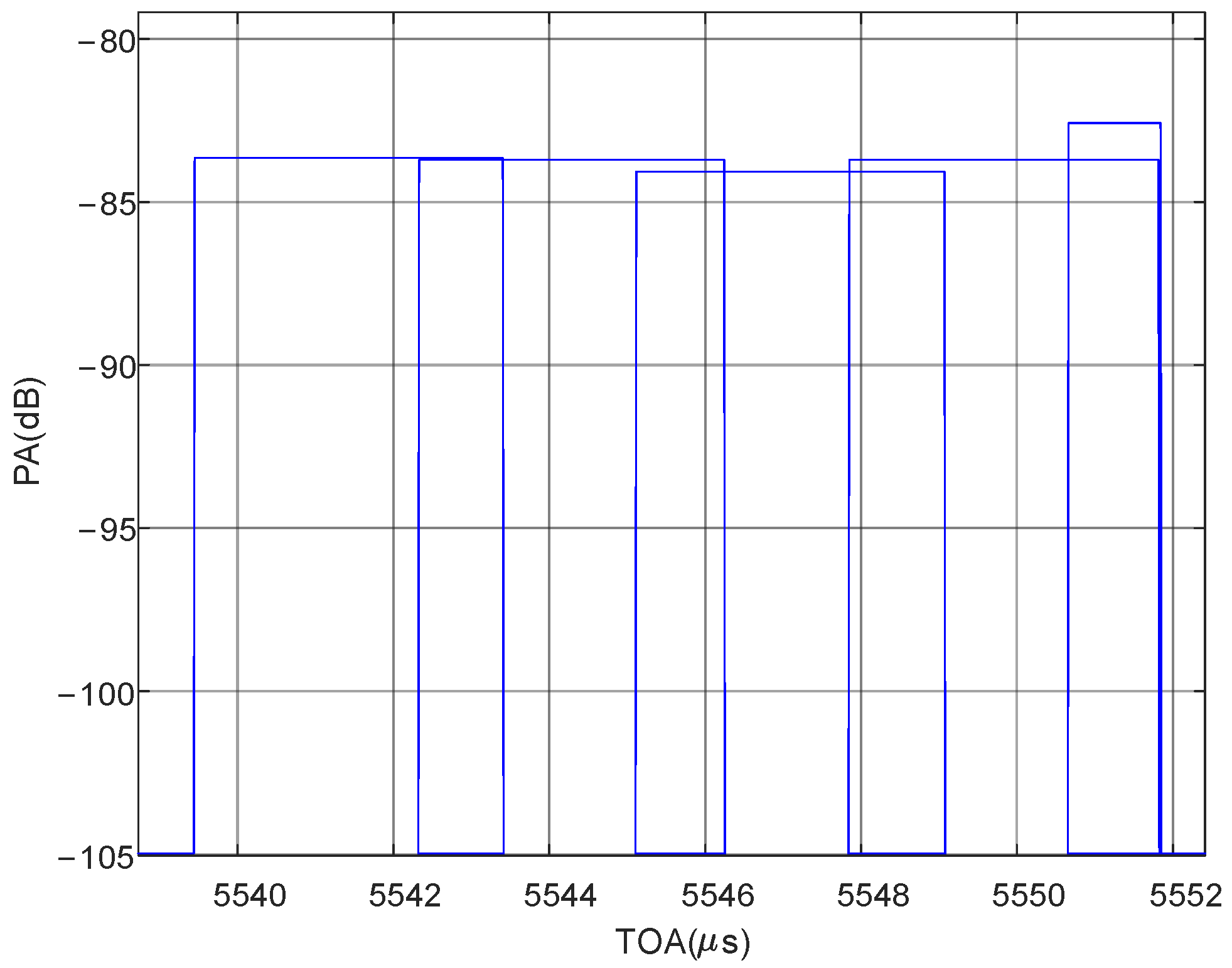
When channelizing a wideband signal, such as a linear frequency modulation signal, its frequency band often covers multiple subchannels, potentially resulting in the detection of split pulses with different TOAs in adjacent channels. The split pulses detected by multiple channels are plotted on the same graph, revealing the phenomenon known as the cross-channel signal split with the split sites located in the time domain corresponding to the transition bands between subchannels. The schematic diagram and the time domain diagram of the experimental data are shown in Figure 2 and Figure 3.
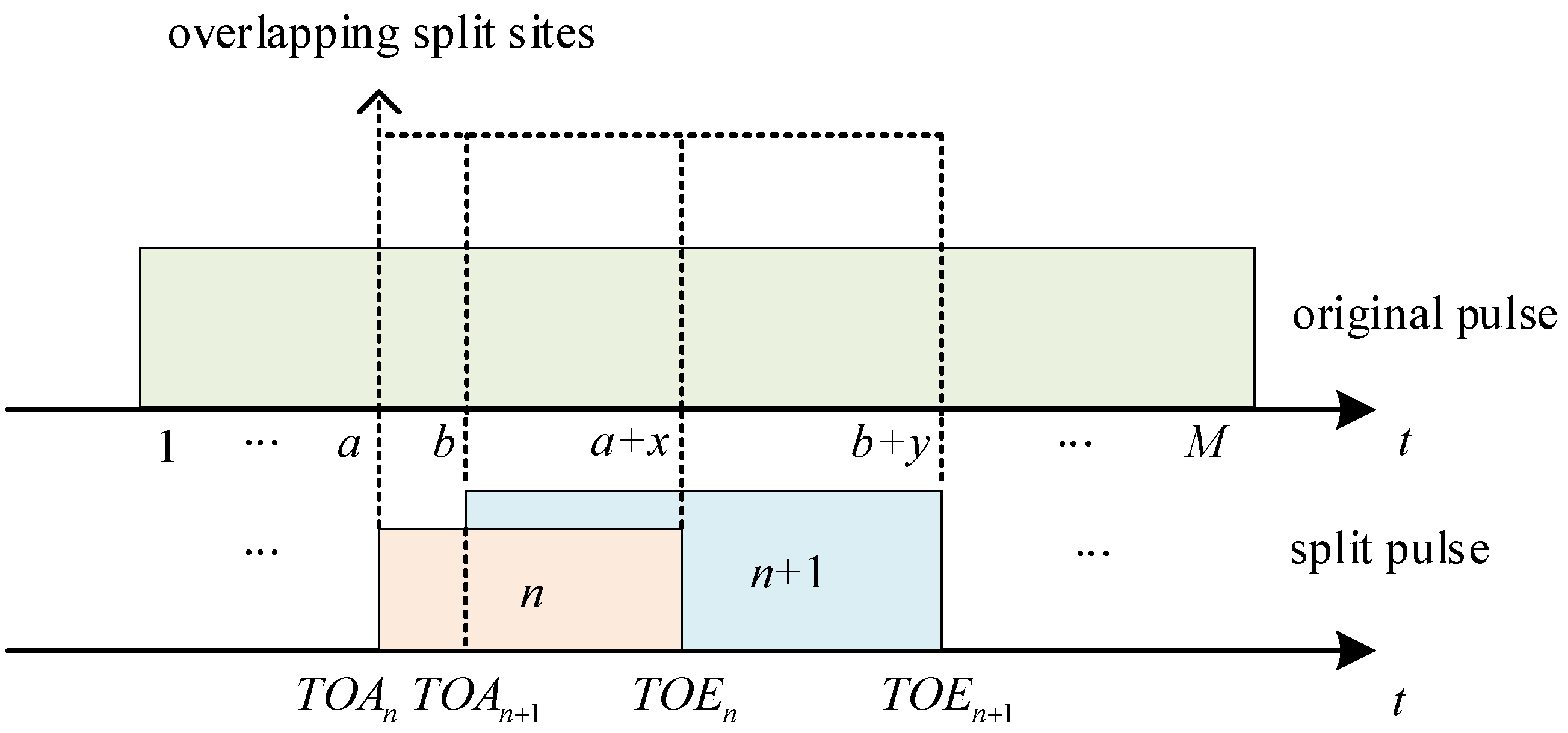
1 M in the upper timeline of Figure 4 represent the split sites of the original pulse. The split sites are denoted as a, b, a + x and b + y , which correspond to the overlapping split sites of the leading edge T O A n , T O A n + 1 , and the trailing edge T O E n , T O E n + 1 of the nth and n + 1 th split pulse in the lower timeline. The timing relationship between the leading and trailing edges of adjacent split pulses and the size of split sites must satisfy the following condition:
T O A n < T O A n + 1 < T O E n < T O E n + 1 a < b < a + x < b + y M
  • Rabbit Ear Effect
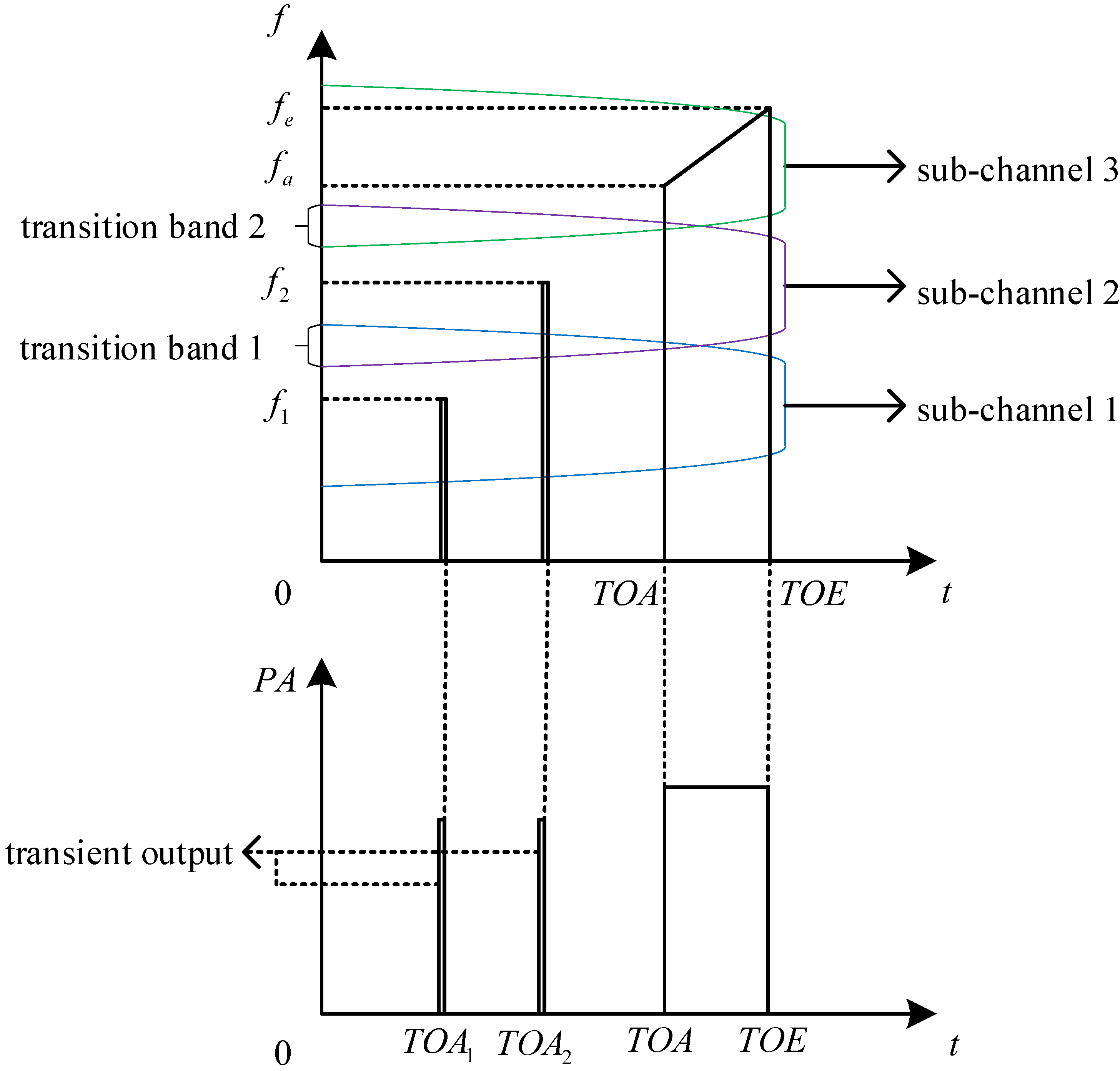
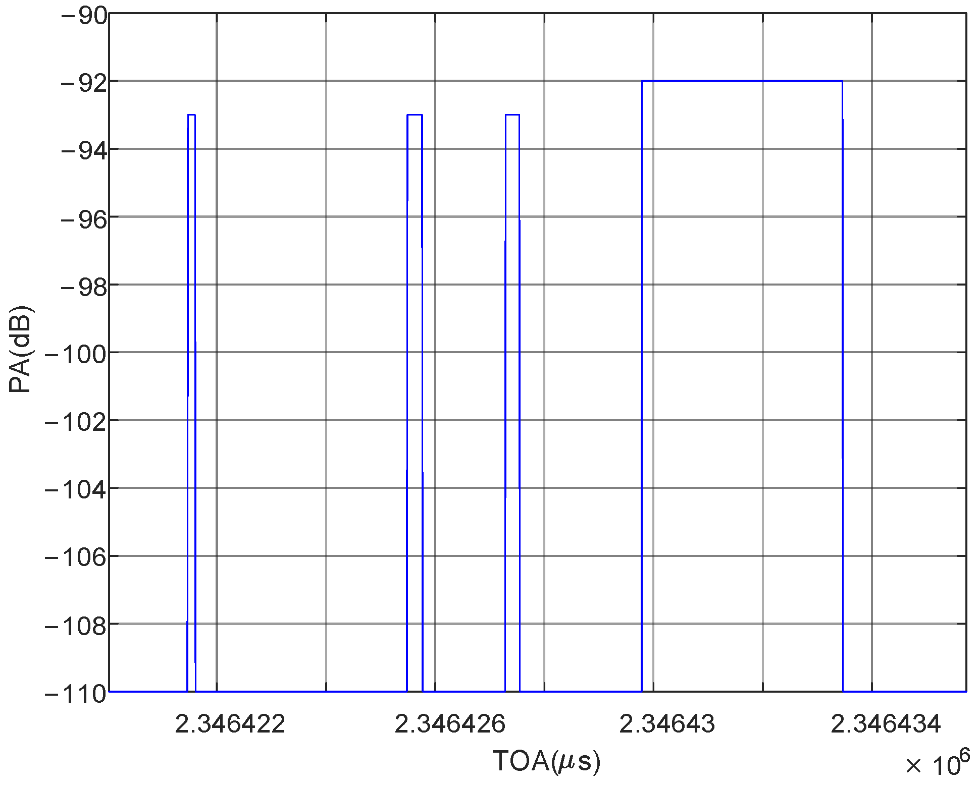
Due to the abrupt change in PA and phase near the rising and falling edges of the pulse signal, channelization will spread the energy of the abrupt change to several subchannels near the actual output subchannel of the signal, resulting in a waveform similar to the transient output of a rabbit ear. The rabbit ear effect appears near the beginning or end of the main signal. The PW is much smaller than the main signal PW, and the PA is slightly smaller as well. Additionally, the adjacent split pulses are independent in the time domain. The schematic diagram and the time-domain diagram of the experimental data are shown in Figure 5 and Figure 6.
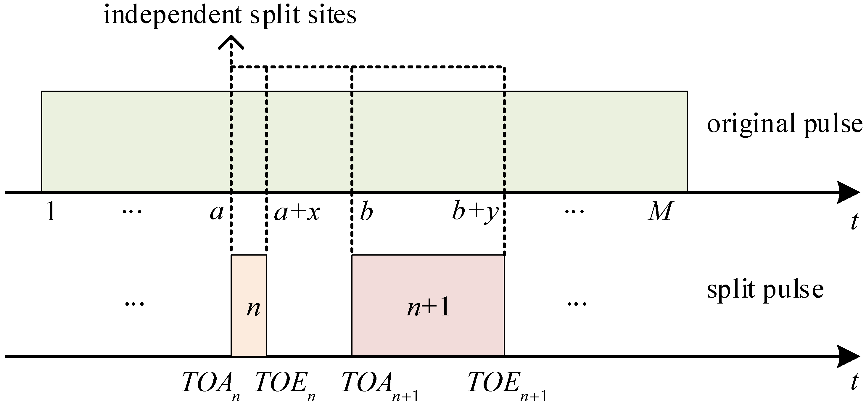
Similar to Figure 4, the upper timeline of Figure 7 shows independent split sites labeled as a, b, a + x , and b + y . These split sites correspond to the leading edge T O A n , T O A n + 1 , and trailing edge T O E n , T O E n + 1 in the lower timeline. The timing relationship of adjacent split pulses and the size of split sites satisfy the following:
T O A n < T O E n < T O A n + 1 < T O E n + 1 a < a + x < b < b + y M
  • Transition Band Repeated Signal
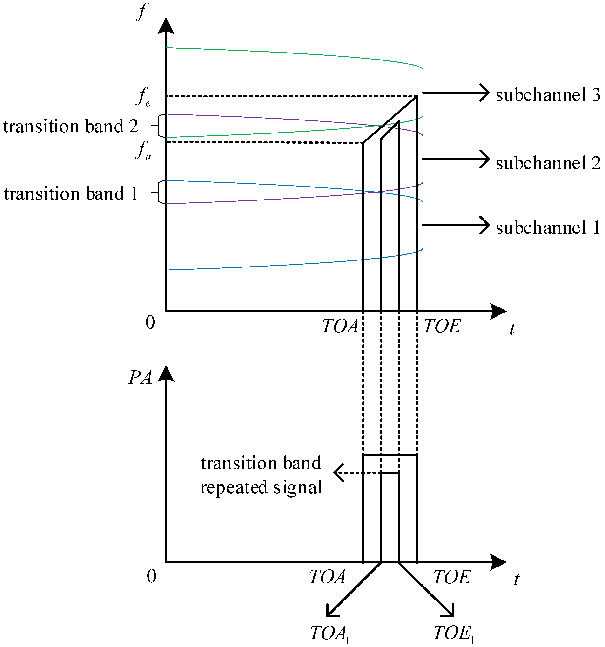
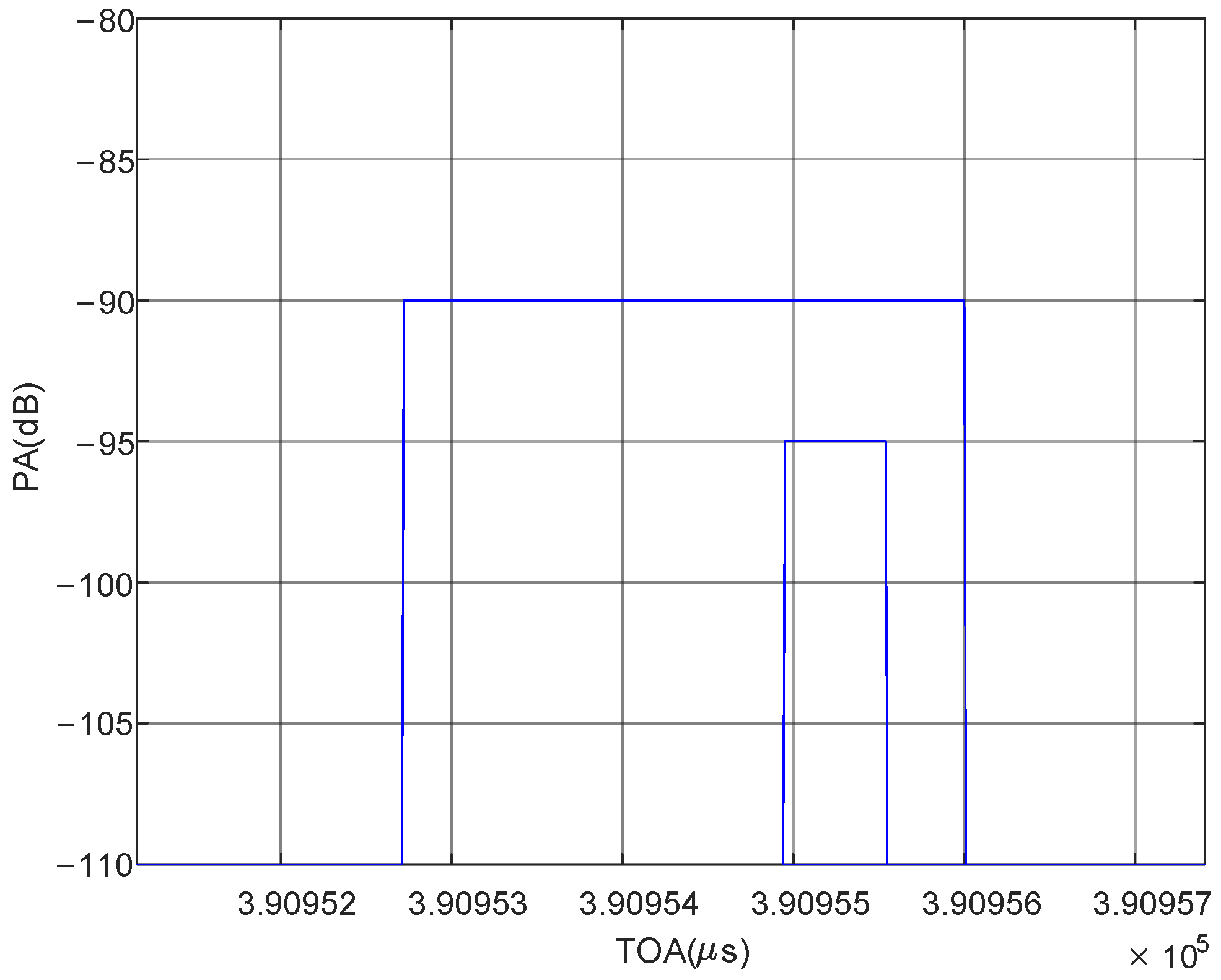
When the signal frequency is located at or near the intersection of adjacent subchannels, it may appear almost simultaneously in two adjacent subchannels, leading to repeated signals in the transition band. Its PA is slightly smaller than that of the real signal, and its leading edge and trailing edge arrival times are approximately the same as those of the real signal. In the time domain, it is mostly encompassed by the real signal. The schematic diagram and time-domain plot of experimental data are shown in Figure 8 and Figure 9.
Similar to Figure 4, the upper timeline of Figure 10 shows mutually contained split sites, which are represented by a, b, a + x , and b + y . These split sites correspond to the leading edge T O A n , T O A n + 1 , and trailing edge T O E n , T O E n + 1 in the lower timeline. The timing relationship of adjacent split pulses and the size of split sites must satisfy the following:
T O A n < T O A n + 1 < T O E n + 1 < T O E n a < b < b + y < a + x M
  • Split PDW Value Range
The range of PDW values corresponding to the split original pulse is given below.
(1) Carrier Frequency
The carrier frequency at the split site has a value range of f s i t e [ f m i n o , f m a x o ] , generating M random values f s i t e that follow a uniform distribution.
(2) PW
The value range of split PW is τ b [ τ m i n , τ o ] , and τ m i n is the minimum value of split PW, generating N random values τ b that obey a uniform distribution.
(3) Arrival Time Front and Back Edge
Let the original pulse arrival time front edge be T O A o , the back edge be T O E o , and the split pulse front site range be denoted as T O A b [ T O A o , T O E o τ m i n ] , where T O E o τ m i n represents the maximum arrival time front that the last split pulse can take. The range of the split pulse back edge site T O E b [ T O A o + τ m i n , T O E o ] , where T O A o + τ m i n represents the minimum arrival time back edge that the first split pulse can take. Then, N random values values for T O A b and T O E b are generated, which follow a uniform distribution.
(4) PA
The original PA is P A o , the corresponding split PA range is denoted by P A b [ P A m i n , P A o ] , and P A m i n represents the minimum value that the split PA can reach, generating N random integers P A b that follow a uniform distribution.

2.1.2. Split Pulse Signal Model

When the original pulse splits in the manner described above, this section provides a mathematical description of the pulse-splitting phenomenon and develops a model for the split pulse signal by constructing the original pulse signal model.
Let the pulse number of the observed original pulse stream be 1 , , e , , E , and the pulse envelope shape is assumed to be ideal, resembling a rectangle. The type of modulation within the pulse is not limited. Therefore, the signal model of the e th original pulse can be expressed as shown below:
s e ( t ) = A e · r e c t ( t T O A e τ e 2 τ e ) · cos ( ω 0 t + ϕ ( t ) )
where r e c t ( · ) represents the unit rectangular window function, A e denotes the PA, T O A e refers to the TOA, τ e represents the PW, ω 0 represents the angular frequency of the signal, and ϕ ( t ) represents the modulation phase of the signal pulse.
A splitting pulse signal model is then constructed based on the original pulse signal model. The sequence number of N splitting pulses generated by the eth original pulse is 1 , , n , , N , the intra-pulse modulation type is consistent with the original pulse. The signal model of the nth split pulse is expressed as:
s e , n ( t ) = A e , n · r e c t ( t T O A e , n τ e , n 2 τ e , n ) · cos ( ω 0 t + ϕ ( t ) )
where A e , n represents the PA of the splitting pulse, T O A e , n denotes the TOA of the splitting pulse, and τ e , n refers to the width of the splitting pulse.

2.1.3. Statistical Model of Split Pulse Number Based on Geometric Distribution

Through the analysis of the experimental data, it is known that pulses transmitted by the same radar and pulses transmitted by different radars will produce a different number of split pulses when passing through the receiver. Count the number of original pulses corresponding to different split pulse numbers from the same radar:
F ( N = 1 ) = F 1 F ( N = 2 ) = F 2 F ( N = l + 1 ) = F l + 1
The value range of the number of split pulses corresponding to the original pulse of this radar is represented by 1 , , l + 1 . F 1 represents the number of original pulses without splitting, and F l + 1 represents the number of original pulses with the maximum number of split pulses l + 1 .
It can be inferred that the number of split pulses follows a geometric distribution based on statistical analysis and practical significance. Therefore, a statistical model of the number of split pulses based on the geometric distribution is constructed. First of all, the probabilities of success and failure of events in the context of the pulse split problem, which are based on the n-weight Bernoulli experiment, need to be explained. The random variable X is defined to follow a Bernoulli distribution with parameter p ( 0 , 1 ] . X can take on the values 1 and 0, representing whether the split pulse can form a complete pulse or not. p ( 0 , 1 ] indicates the probability that each split pulse can form a complete pulse. The distribution law is as follows:
P ( X = 1 ) = p P ( X = 0 ) = 1 p = q
Here, p ( 0 , 1 ) , P ( X = 1 ) represents the probability that the split pulse can form a complete pulse, and P ( X = 0 ) represents the probability that the split pulse cannot form a complete pulse. In addition, when p = 1 , the split pulse is the complete pulse.
Based on the above setting, let L random variables X 1 , , X l , X l + 1 , , X L be independent and identically distributed according to the Bernoulli distribution with parameter p ( 0 , 1 ] . The random variable Y is defined as follows: for any l F , Y = l is true if and only if X 1 = X 2 = = X l = 0 and X l + 1 = 1 hold, where X 1 = X 2 = = X l = 0 indicates that the 1 l -th split pulse cannot form a complete pulse, and X l + 1 = 1 indicates that the l + 1 -th split pulse can form a complete pulse. Then, the event Y = l means that its neighboring l split pulses cannot form a complete pulse until the l + 1 th split pulse arrives. When the l + 1 th split pulse appears, it successfully forms a complete pulse with the first l split pulses exactly. The distribution law of the random variable Y is as follows:
P ( Y = l ) = ( 1 p ) l · p , l F
  • Effect of PW and PA on Split Pulse Number
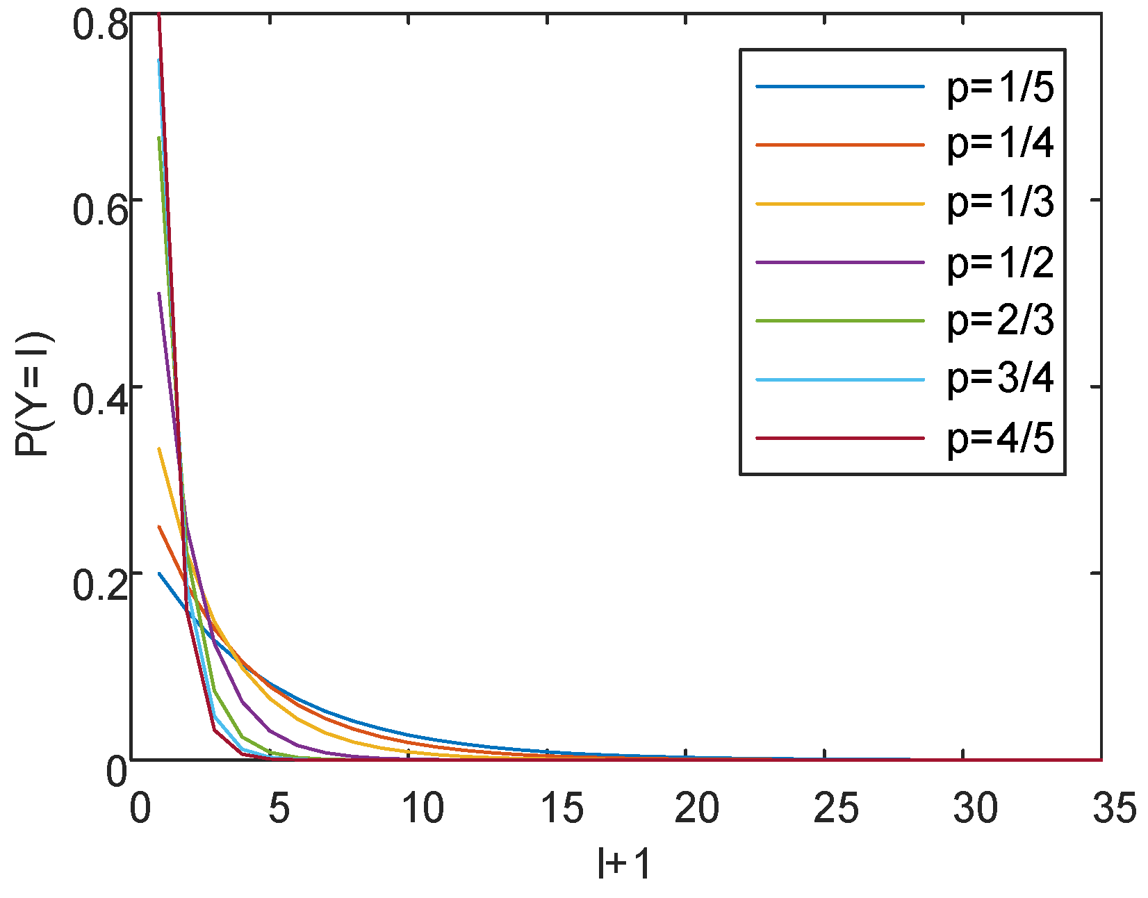
As shown in Figure 11, the p values of different radars vary due to differences in parameters such as PW and PA. The higher the probability p that the split pulse constitutes a complete pulse, the larger the average slope | k | of the curve, and the faster the curve declines simultaneously. The minimum P i n f = 1.5 × 10 4 close to 0 is set as the discriminative threshold for determining the maximum number of split pulses needed to successfully construct a complete pulse. P ( Y = l 1 ) > P i n f if and only if P ( Y = l ) < P i n f . In this case, the abscissa l + 1 represents the maximum number of split pulses required for the radar to form a complete pulse. The calculated results are shown in Table 2. It is clear that the larger the value of p, the fewer split pulses are needed to form a complete pulse.
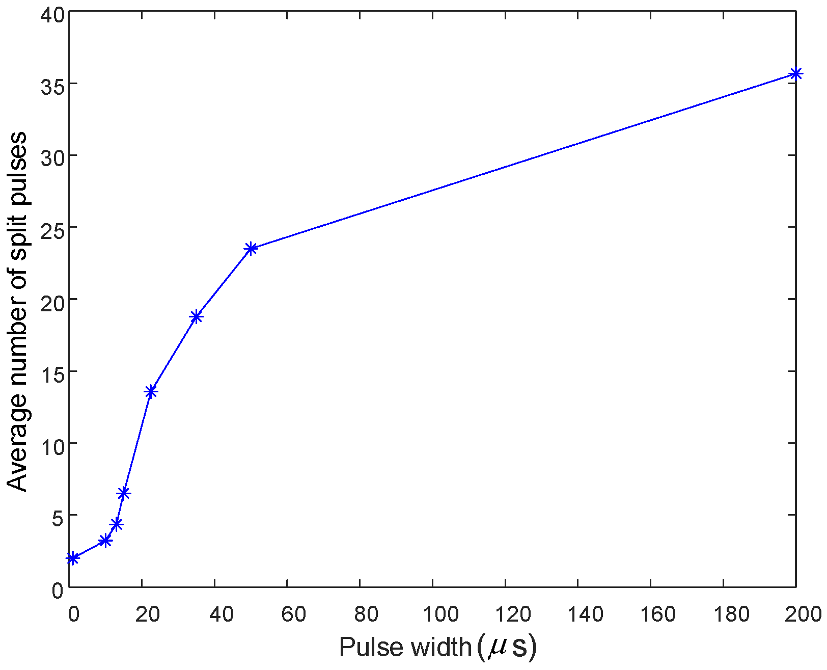
Then, the influence of PW on the splitting of pulses is discussed. The experimental data are used to calculate the average number of splitting pulses corresponding to different PWs. The results are shown in Figure 12, which indicates that the average number of splitting pulse increases as the PW increases. According to Table 2, the smaller the probability p of the split pulse forming a complete pulse, the flatter the corresponding curve of the geometric distribution law becomes.
Finally, the influence of PA on pulse splitting is analyzed. The experimental data of pulse splitting from the same radar are selected to calculate the average number of pulse splitting with the same PW but different PA. As shown in Figure 13, the average number of pulse splitting gradually decreases with the increase in PA until it remains unchanged after reaching −82 dB. Assuming that the ambient noise of the receiving device does not change over time, the radar pulse SNR is primarily influenced by the PA. The larger the PA, the less impact pulse splitting has on the environment, and the smaller the maximum number of pulse splitting required to form a complete pulse. Combined with Table 2, it can be observed that as the probability p of the split pulse forming a complete pulse increases, the curve of the geometric distribution law becomes steeper.

2.2. Building the Split Pulse Flow

According to the generation mechanism of split pulse, the split pulse signal model, and the statistical model of split pulse number, a split pulse flow is constructed to verify the performance of the split pulse detection method described below. The pulse flow density, pulse splitting degree, pulse staggering degree, and pulse recurrence interval (PRI) modulation complexity are defined as characteristics of pulse flow to describe the changing pattern of split pulse flow in a complex environment.

2.2.1. Pulse Flow Density

Pulse flow density ρ is defined as the number of pulses received by the receiver per unit time and can be expressed as shown below:
ρ = N p T f
where N p is the number of pulses received within a given timeframe, and T f represents the duration of that timeframe.
The pulse flow density can be reflected by the length of the pulse repetition interval. U radars are assumed to transmit pulse streams with densities P = [ ρ 1 , , ρ u , , ρ U ] successively over time. The general formula for calculating pulse flow densities is as follows:
ρ u = 1 P R I u
The PRI of the radar u pulse stream is P R I u , and the pulse flow density ρ u is the reciprocal of P R I u . The split PDW datasets with different pulse flow densities are generated by combining the pulse-splitting model with other pulse flow characteristics unchanged.

2.2.2. Pulse-Splitting Degree

The degree of pulse splitting P ( X = 0 ) = q , q [ 0 , 1 ) is defined as the probability that split pulses cannot form a complete pulse. As can be seen from Figure 11 and Table 2, the larger q is, the higher the maximum number of split pulses required to form a complete pulse. Suppose that when receiving the pulse streams arriving successively from the same radar, the corresponding pulse splitting degree is Q = [ q 1 , , q u , , q U ] . The split PDW datasets with varying degrees of pulse splitting are generated by combining the pulse-splitting model with other unchanged pulse flow characteristics.

2.2.3. Pulse Staggering Degree

The pulse staggering degree R N is defined as the number of radars receiving the pulse stream within a given timeframe. The higher the number of radars, the greater the pulse staggering degree. Set the staggering degree corresponding to the arriving pulse streams as RN = [ R N 1 , , R N u , , R N U ] . Keep the characteristics of other pulse streams unchanged and combine the pulse-splitting model to generate split PDW datasets with different pulse staggering degrees.

2.2.4. PRI Modulation Complexity

The PRI modulation complexity c is defined as the modulation type of the PRI corresponding to the radar pulse stream within a basic timeframe. The higher the complexity of the modulation type, the higher the PRI modulation complexity. Set the modulation complexity of the PRI corresponding to the incoming pulse streams as c = [ c 1 , , c u , , c U ] . Keep the characteristics of other pulse streams unchanged and combine the pulse-splitting model to generate split PDW datasets with varying PRI modulation complexities.

2.2.5. Integrated Pulse Flow Characteristics

Let the pulse flow density, pulse-splitting degree, pulse-staggering degree, and PRI modulation complexity, which change simultaneously in a time sequence, be:
M = ρ 1 ρ u ρ U q 1 q u q U R N 1 R N u R N U c 1 c u c U
Combined with the pulse-splitting model, a split PDW dataset is generated, which exhibits multiple pulse flow characteristics changing simultaneously.

2.2.6. Reference Label Generation Method

The generation method for timeframes with reference labels is described as follows: First, the original PDW dataset is generated, and then different numbers of split pulses corresponding to the original PDW are generated according to the pulse-splitting model. The original PDW data with split pulse numbers is processed in frames, and the timeframes are labeled according to Table 3.

3. Split Pulse Detection

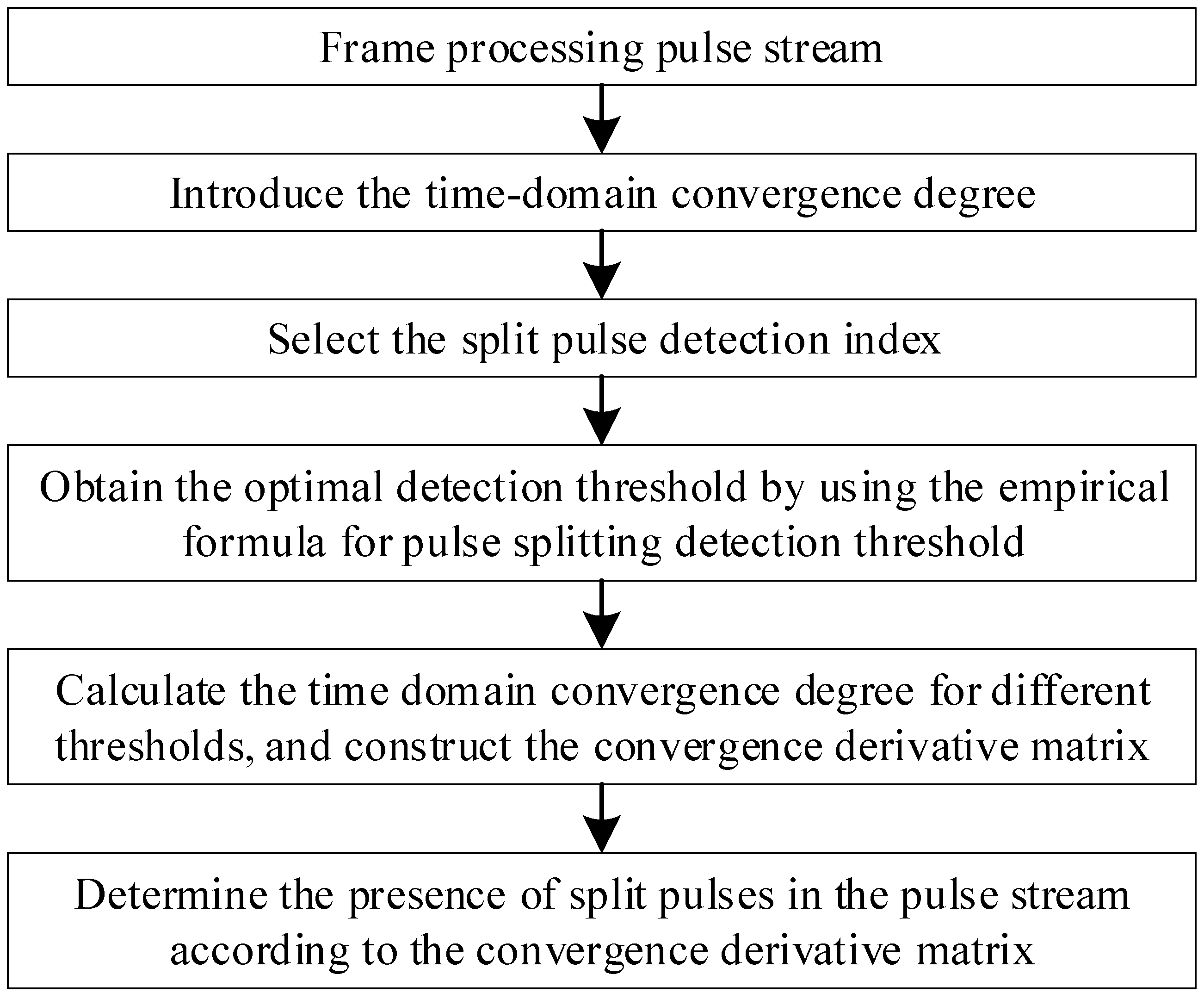
A method for detecting splitting pulses based on a split pulse model is proposed. Firstly, the pulse stream is divided into frames of equal length, and then the degree of convergence in the time domain is introduced to characterize the splitting of pulses. An empirical formula for determining the detection threshold based on the convergence degree in the time domain is provided to obtain an appropriate threshold for each timeframe. Formed by calculating the derivatives of the convergence degree in the time domain at adjacent thresholds, the convergence derivative matrix is used to efficiently identify any potential splitting problems in the pulse flow. The flow of the algorithm is shown in Figure 14.

3.1. Framing the Pulse Stream

The pulse stream with a timeframe length T f is the fundamental processing unit of the split pulse detection algorithm and is calculated as follows:
T f = T P D W N f
where T P D W is the duration of interception time for PDW and N f is the number of timeframes. The processing of pulse stream framing can reduce the algorithm’s processing time, enabling the localization of split pulse detection within each timeframe and facilitating the subsequent processing of timeframes containing split pulses.

3.2. TCD

In order to determine whether there is a split pulse in each frame, this paper introduces the full-window standard deviation (FSTD) based on the standard deviations. It then improves the single-box moving step of FSTD to a multi-box moving step of independent full-window standard deviations (IFSTD). Finally, the concept of TCD is introduced, which is a statistical distribution.
The standard deviation S can reflect the dispersion of a dataset and is expressed as follows:
S = S 2 = 1 V 1 v = 1 V ( X v X ¯ ) 2
where X v , v = 1 , , V represents each sample of the dataset, X ¯ denotes the sample mean, and V represents the sample size. The smaller the standard deviation, the more stable the dataset.
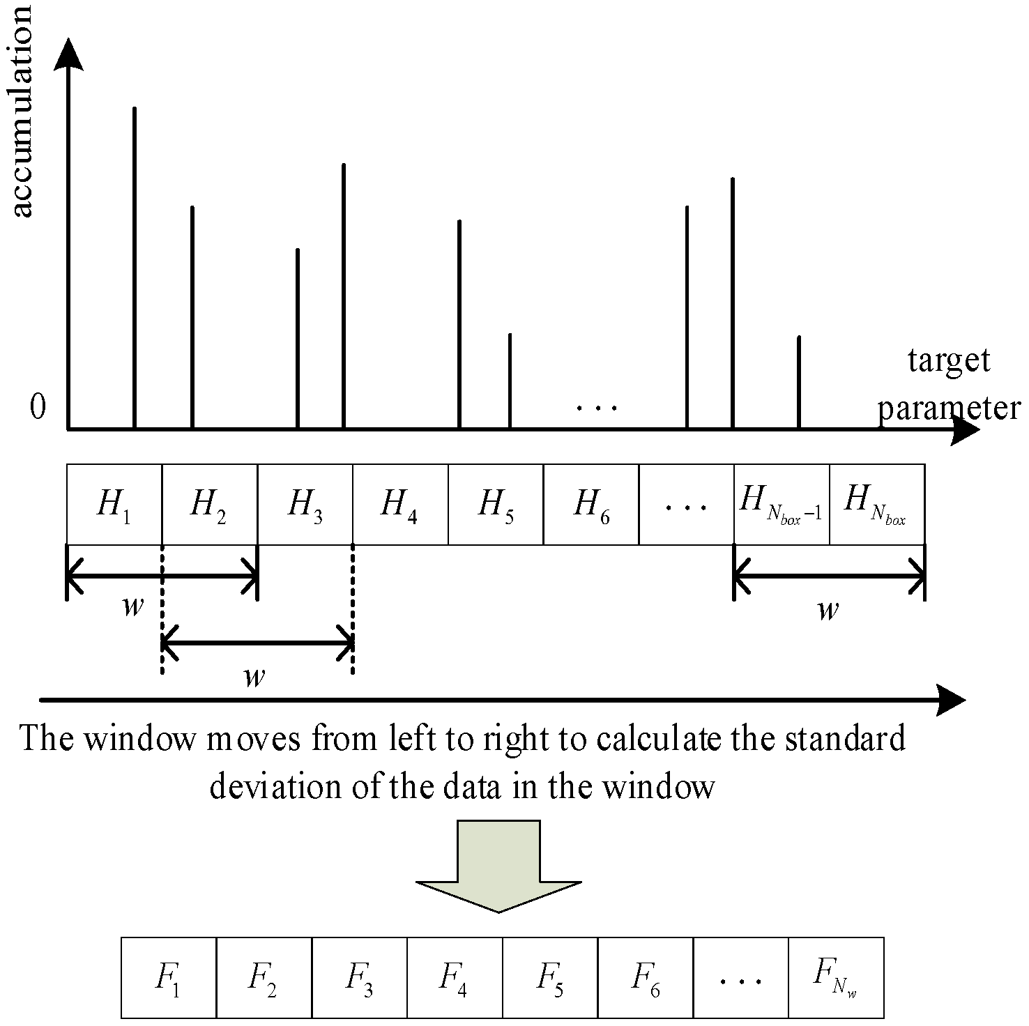
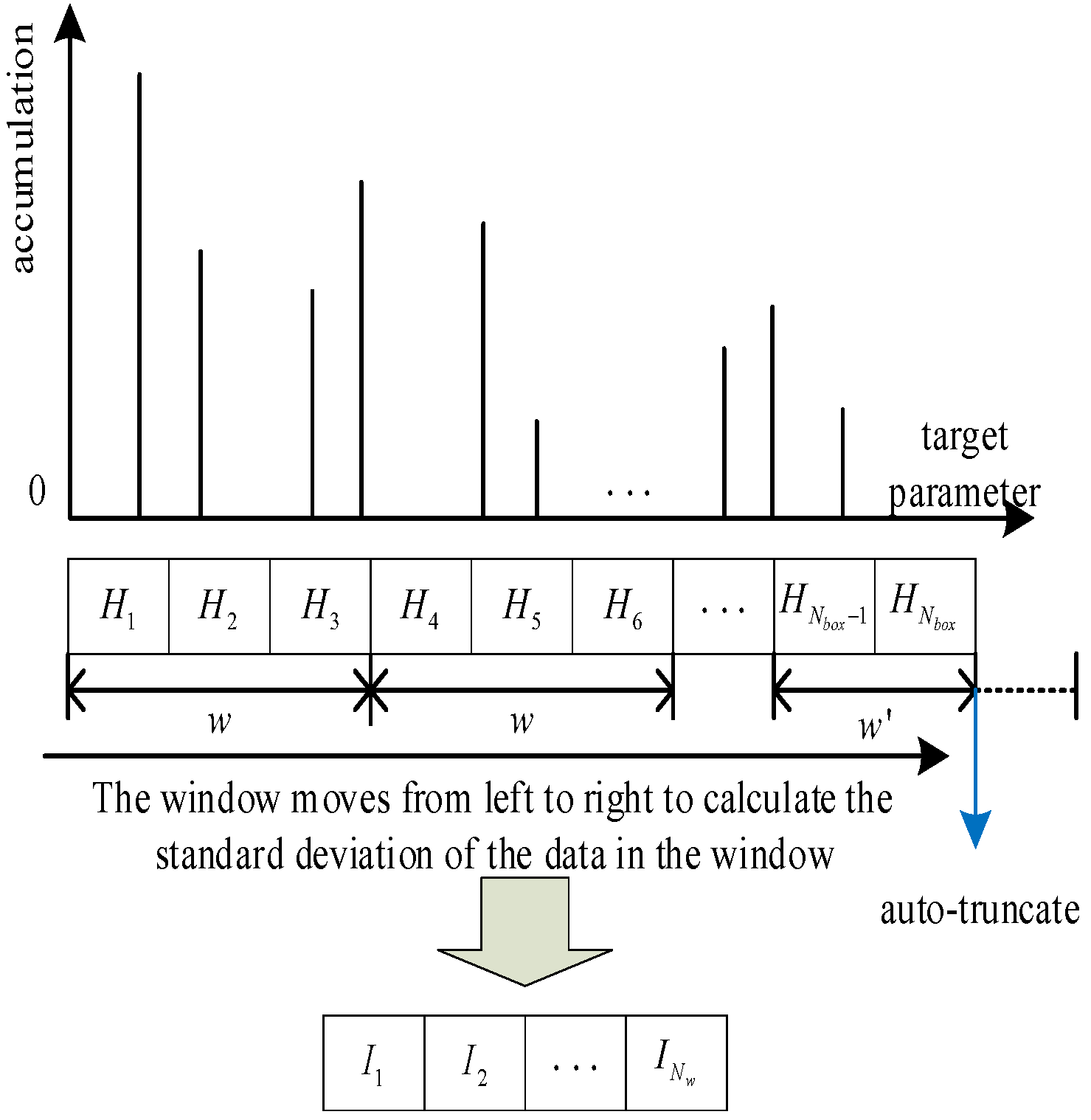
As shown in Figure 15, the standard deviation of the window length for a fixed value w (referred to as the FSTD) is calculated sequentially for each box in the histogram, starting from the left and moving toward the right along the horizontal coordinate. When each FSTD is calculated, the window will shift to the right by the length of a single box. Here is how to calculate each FSTD:
F j = i = j j + w 1 ( H i H ¯ j ) 2 w 1
where the pulse cumulant per box (histogram height) is H i , i = 1 , , N b o x , and N b o x represents the number of boxes in the radar pulse flow parameter histogram. The mean height of the histogram in the window is H ¯ j , j = 1 , , N w , and N w = N b o x ( w 1 ) is the number of windows. The expression can be written as follows:
H ¯ j = i = j j + w 1 H i w
Then, by improving the single-move step length of FSTD to the window length, TCD is introduced into the calculation to represent the convergence of the pulse stream parameter distribution histogram. As shown in Figure 16, the FSTD is calculated from left to right along the abscissa with a fixed window length and independent coverage of the histogram, which is defined as IFSTD. When calculating each IFSTD, the window will shift w elements to the right. When calculating the last IFSTD, the window will automatically truncate at the end of the abscission value. IFSTD is calculated as follows:
I j = i = ( j 1 ) w + 1 j w ( H i H ¯ j ) 2 w 1 , j < N w I j = i = ( N w 1 ) w + 1 N b o x ( H i H ¯ N w ) 2 w 1 , j = N w
IFSTD reflects the standard deviation of each window length in the parametric histogram, and the results obtained are more independent and significant compared to FSTD. Finally, IFSTD is averaged to obtain the TCD:
T C D = j = 1 N w I j N w
The histogram window number is N w = N b o x w , and the meaning of the remaining variables is consistent with the description provided above.

3.3. Split Pulse Detection Indicator

In order to perform split pulse detection on the received PDWs, the following time domain indicators are selected to draw the histogram and calculate the TCD.
  • PW
The PW ( τ ) is the duration for which the pulse can reach its maximum value.
  • Duty Cycle (DC)
DC (D) is the ratio of PW to the adjacent pulse time interval ( D T O A ):
D = τ D T O A
For split pulses, the calculation of the DC can be divided into two cases: pulse independence and pulse non-independence. For independent splitting pulses, as shown in Figure 17, the sequential relationship between adjacent splitting pulses is T O A d + 1 > T O A d + τ d , and the DC calculation method is consistent with Equation (19): D d = τ d / D T O A d = τ d / [ T O A d + 1 T O A d ] . For splitting pulses that are not independent of each other, as shown in Figure 18, the sequential relationship between adjacent splitting pulses is T O A n + 1 < T O A n + τ n , n = d , z , and the DC D d = D z = 1 of pulses d and z is specified. In particular, as shown in Figure 19, if the current timeframe has only one pulse, the DC of the pulse is specified as the ratio of the PW to the current timeframe length D i = τ i / T f .
The degree of convergence of PW and DC in the time domain over a period of time can indicate the splitting of the pulse train. Therefore, these parameters are used as indicators to measure whether the pulse train is split.
TCD can reflect the extent of overlap and splitting of the pulse flow. Take PW as an example. As shown in Figure 20, for a complete pulse flow, the TCD calculated from the PW distribution histogram is lower. As shown in Figure 21 and Figure 22, the TCD calculated from the PW distribution histogram is larger for overlapping or splitting pulse flows.

3.4. Empirical Formula of Splitting Pulse Detection Threshold

The difficulty of the algorithm lies in selecting the appropriate detection threshold for each PDW frame to achieve high accuracy in split pulse detection. In order to clarify the measurement object of the detection threshold t h s , the missing pulse length T g is defined as the time difference between the arrival time of the back edge of the first arrival pulse and the arrival time of the front edge of the second arrival pulse [16]. It can be expressed as follows:
T g = T O A n + 1 T O E n
where T O A n + 1 is the arrival time of the front edge of the second arrival pulse, and T O E n is the arrival time of the back edge of the first arrival pulse. As shown in Figure 23, it can be seen that within a given timeframe, the number of missing pulse lengths is one less than the number of splitting pulses. In order to facilitate matrix calculation, the first splitting pulse and the second splitting pulse share the same missing pulse length T g 1 = T g 2 to ensure that the number of missing pulse lengths is consistent with the number of splitting pulses.
For split pulses, T g is calculated differently when the pulses are independent of each other and when they are not independent of each other. For independent splitting pulses, as shown in Figure 17, T g is calculated in the same way as Equation (20). For split pulses that are not independent of each other, as shown in Figure 18, the missing pulse length of pulses t and z is specified as T g t = T g z = 0 . In particular, as shown in Figure 19, if the current timeframe has only one pulse, the missing pulse length T g i is equal to 0.
Calculate the absolute difference between the mean missing pulse length and the mean PW of each PDW frame, multiply this absolute value by the mean duty ratio, and round the result to obtain the empirical formula for the detection threshold of split pulses. The mean values of the missing pulse length ( T g ), PW ( τ ), DC (D) and the detection threshold for split pulses ( t h s m a x ) are calculated as follows:
T g ¯ = i = 1 n b ( D T O A i τ i ) n b
τ ¯ = i = 1 n b τ i n b
D ¯ = i = 1 n b 1 τ i D T O A i n b 1
t h s m a x = r o u n d ( | T g ¯ τ ¯ | × D ¯ )
where r o u n d ( x ) is the rounding function used to ensure that the reasonable detection threshold t h s m a x of each frame PDW is an integer. The reasonable detection threshold of each frame data is t h s m a x . T g i , τ i , D T O A i and D i represent the missing pulse length, PW, adjacent pulse time interval, and DC per frame, respectively. Additionally, n b denotes the number of pulses per frame.
When there are no split pulses within the timeframe, T g ¯ , τ ¯ and | T g ¯ τ ¯ | are relatively large. As the number of split pulses increases, both T g ¯ and τ ¯ gradually decrease, and | T g ¯ τ ¯ | decreases compared to the timeframe with only complete pulses. Coefficient D ¯ ensures that t h s m a x falls within the range ( τ m a x , D T O A m i n o ) in the majority of cases, ensuring accurate and effective detection of split pulses. The number of t h s m a x falling within the ( τ m a x , D T O A m i n o ) range as a percentage of the total number of detection thresholds is consistent with the split pulse detection accuracy, where τ m a x is the maximum pulse width within the frame, and D T O A m i n o is the minimum adjacent pulse time interval between complete pulses.

3.5. Radar Split Pulse Detection Method

The attempts to merge split pulses with different threshold values ( t h s ) are performed on the PDW frame sequentially. If T g < t h s , the adjacent pulses should be merged, and the pulses are considered split pulses. If T g t h s , they should not be merged, and the pulses are considered complete pulses. The detection threshold range t h s [ t h s m i n , t h s m a x ] is set to adjust the pulse detection threshold incrementally from small to large with a fixed step size. Usually, the starting threshold t h s m i n = 0 is set to indicate that pulse merging is not performed.
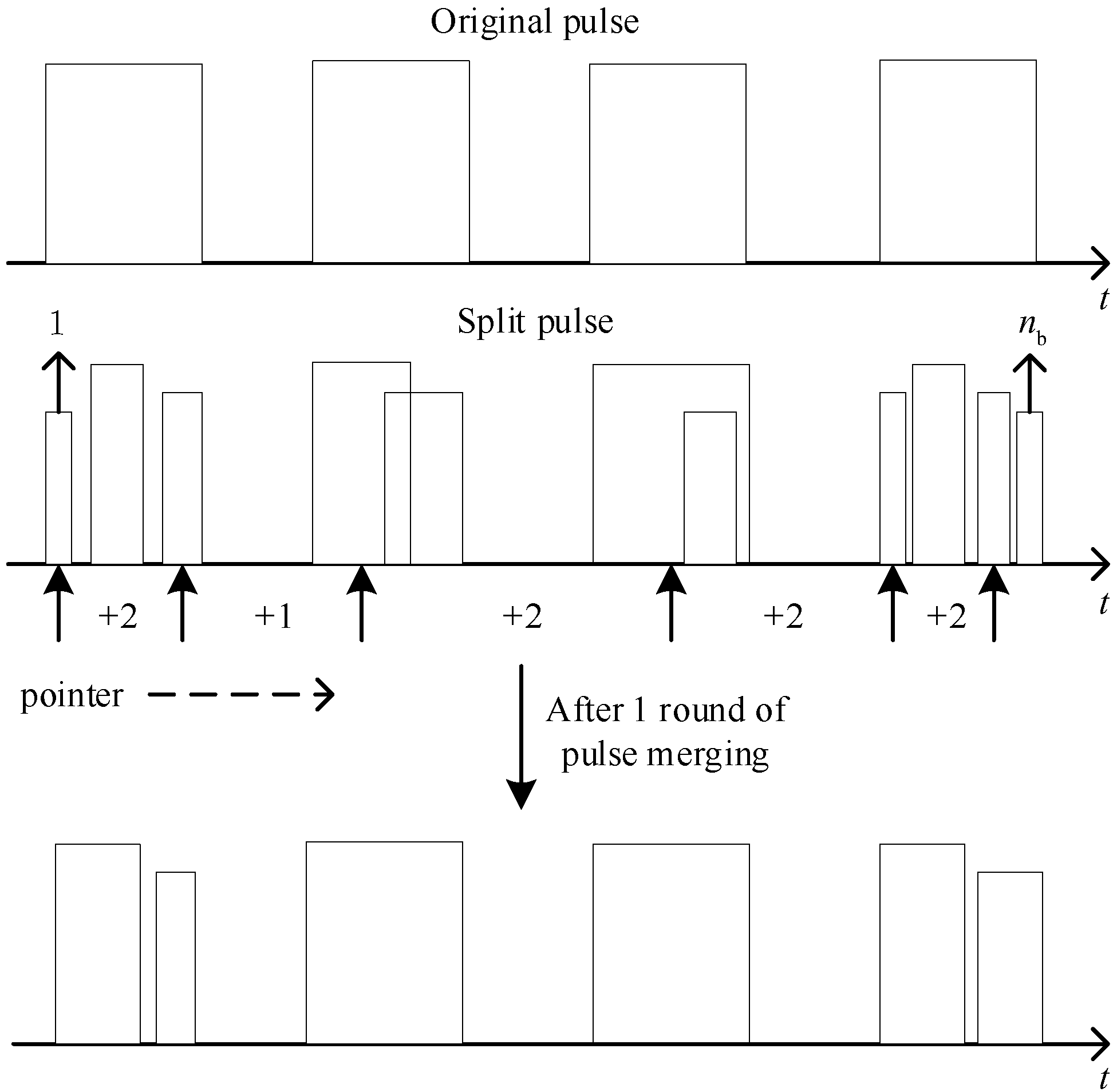
As shown in Figure 24, the number of pulses in each timeframe can be set as n b , and the pulse merging processing pointer is positioned to the current pulse i , i [ 1 , n b 1 ] that needs to be processed. If the current pulse, denoted by the pulse merging processing pointer, and the next pulse i + 1 satisfy the merging condition, the pulses will be merged. Otherwise, the original state of the pulse will remain unchanged. Then, the position of the pulse merging processing pointer is updated, and the search for the next pulse that satisfies the pulse merging condition continues until the pointer points to the pulse with sequence number n b 1 , indicating that the merging process is complete. Then, the position of the pulse merging processing pointer is updated to locate the next pulse that satisfies the pulse merging condition until the pointer points to the pulse with sequence number n b 1 .
According to the given rules, the PDW sequences generated by different detection thresholds are merged. The PW dimension of the merged PDW sequence is extracted, and the DC dimension is calculated using Equation (19). The histogram of the PW and DC dimensions is plotted, and the time domain convergence degree is calculated to create the time domain convergence degree matrix:
TCD = [ T C D 1 , , T C D i , , T C D I ]
where i = 1 , , I is the sequence number of the detection threshold. Finally, the convergence degree of adjacent detection thresholds in the time domain is derived to reflect the change rate k i , i + 1 of a fixed step size m:
k i , i + 1 = T C D i + 1 T C D i m
The results of the derivation are then formed into the time domain convergence degree derivative matrix:
k = [ k ( 1 , 2 ) , , k ( i 1 , i ) , , k ( I 1 , I ) ]
where i = 2 , , I , k ( 1 , 2 ) and k ( I 1 , I ) represent the derivative results of the time domain convergence degree of the first two and the last two detection thresholds, respectively.
According to the above calculation process, the convergence degree derivative matrixes of the PW and DC dimensions are calculated as k τ and k D C . If the time domain convergence degree T C D i remains unchanged, the change rate k ( i , i + 1 ) is equal to 0 and the convergence degree derivative matrices k τ and k D C are all zero matrices with the increase in the detection threshold, indicating that the pulse timing position does not change, and no new merging pulse is generated. If the time domain convergence degree changes, the convergence derivative matrices k τ and k D C are not all-zero matrices, indicating that the new merging pulses are generated. The discriminative labels are generated according to the above algorithm shown in Table 4.

4. Simulation Analysis and Verification

4.1. Parameter Setting

The simulation data in Table 5 and experimental data in Table 6 are derived from multiple radars with fixed PRI, staggered PRI, and group-staggered PRI modulation types. These data are numerically translated based on the original data.
Then, the methods for setting data under various conditions are described.
Pulse flow density: Set the PRI of radars A, B and C to generate different PRI settings, resulting in pulse flow densities of magnitudes in the ranges of [ 10 2 , 10 3 ) , [ 10 3 , 10 4 ) and [ 10 4 , 10 5 ) pulses per second. Only a fixed PRI signal is transmitted. The pulse-splitting degree q is set to 1/3 for each radar, while the pulse-staggering degree R N is kept constant at 1.
Pulse-splitting degree: For radar D, set q = 1 / 4 , 1 / 3 and 1 / 2 to generate different pulse splitting degrees. The pulse flow density ρ remains in the same order of magnitude, with [ 10 3 , 10 4 ) pulse numbers per picosecond. Only a fixed PRI signal is transmitted, and the pulse staggering degree R N is set to 1 remain unchanged.
Pulse-staggering degree: Combine radars E, F and G for interleaving to generate different pulse-staggering degrees within a single frame with R N = 1 , 2 , 3 , respectively. For each radar, the signal with the same pulse-splitting degree q = 1 / 3 and fixed PRI modulation type is set. The data frame is taken with a pulse flow density in the same order of magnitude [ 10 3 , 10 4 ) pulse numbers per picosecond.
PRI modulation cmplexity: Set different PRI modulation complexities for radars H, I and J: fixed PRI, staggered PRI and grouped staggered PRI. Each radar is set with the same pulse flow density order of magnitude [ 10 3 , 10 4 ) pulse numbers per picosecond. Additionally, a pulse-splitting degree of q = 1 / 3 and a pulse-staggering degree of R N = 1 are set for each radar.
Integrated pulse flow characteristics: Set different radar parameters for radars K, L and M with varying pulse flow density, pulse-splitting degree, pulse-staggering degree and PRI modulation complexity to reasonably replicate experimental data in a complex electromagnetic environment.
Experimental data: The labeled experimental data are used to verify the validity of the proposed model and algorithm.

4.2. Verification of the Statistical Distribution of the Split Pulse Number

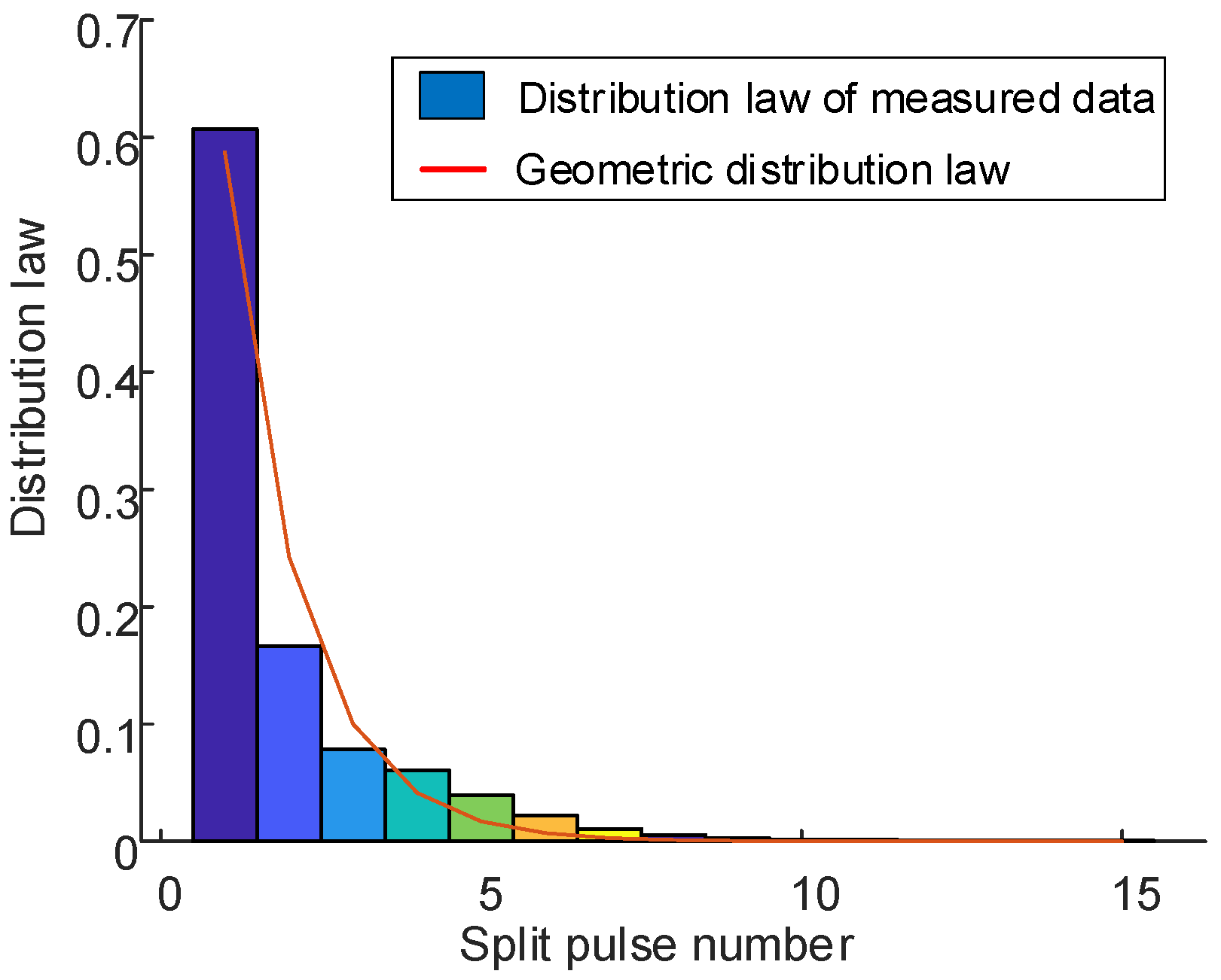
The number of split pulses corresponding to the original pulse is counted using the experimental data from the same radar. The percentage of the original pulse number f i corresponding to the different split pulse number i in the total number E of the original pulse is then calculated. The statistical results are shown in Table 7. The histogram is drawn based on the statistical distribution of the number of split pulses and is compared to the geometric distribution law, as shown in Figure 25.
In order to validate the rationality of the statistical model for split pulse number, the K-S (Kolmogorov–Smirnov) test [19] is employed to determine if the split pulse number of the experimental pulse flow follows a geometric distribution. Let the null hypothesis H 0 to be tested be: the distribution of the split pulse number Y of the experimental pulse flow belongs to the geometric distribution family, i.e., Y G e o ( p ) . It is verified that by accepting H 0 at the significance level α = 0.05 , the distribution of population Y is considered to belong to the geometric distribution family, i.e., Y G e o ( p ) .

4.3. Performance Analysis of Algorithms

This section analyzes whether the variation of window length and frame length affects the split pulse detection result and verifies the validity of the empirical formula used for determining the split pulse detection threshold.

4.3.1. Window Length

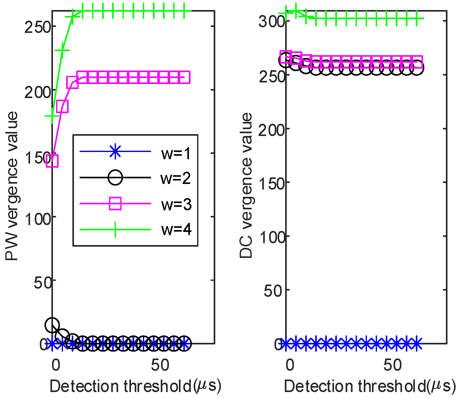
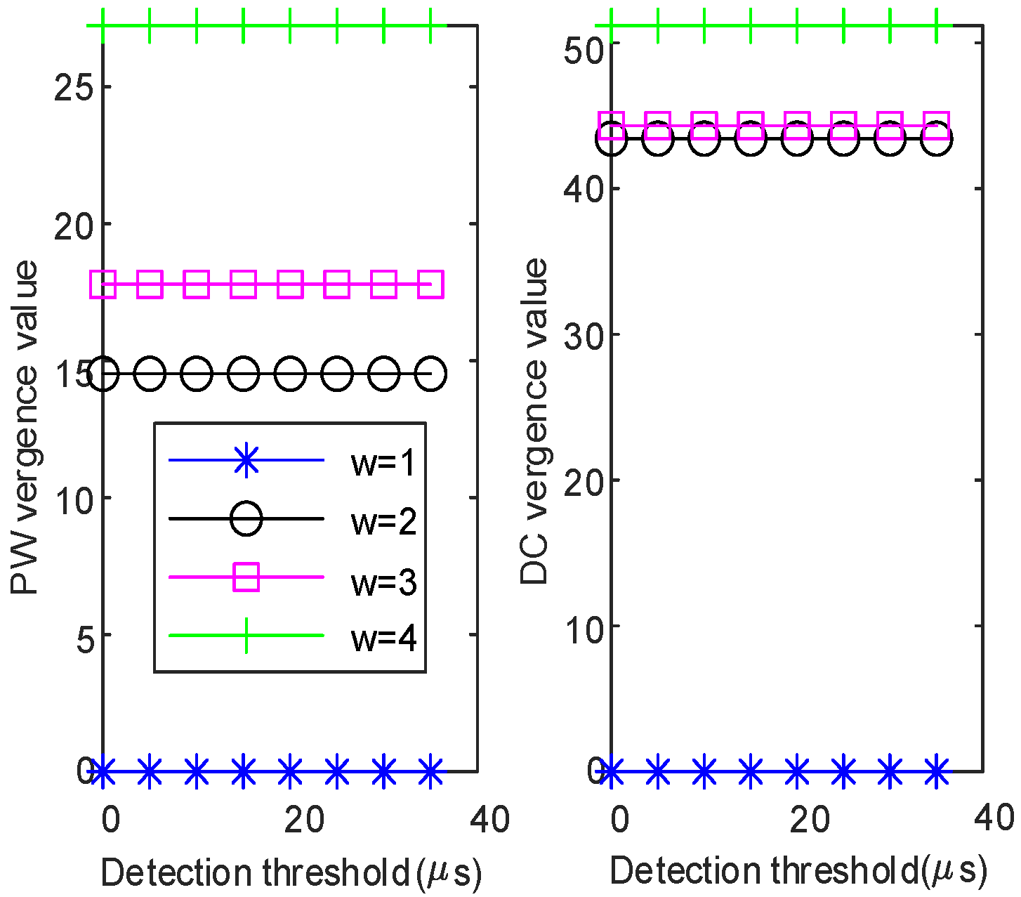
As one of the parameters that determines the level of convergence in the time domain, the window length can be adjusted in the split pulse detection algorithm. Therefore, it is necessary to test whether the degree of convergence in the time domain, as calculated using different window lengths, affects the result of split pulse detection. Keep other parameters unchanged, set the window length as w = 1 , 2 , 3 , 4 , and conduct comparative experiments using simulated data. When w = 1 , as shown in Figure 26 and Figure 27, regardless of whether split pulses exist in the frame, the time domain convergence degree of PW and DC is 0 and does not change with the detection threshold. When w > 1 , as shown in Figure 26, the convergence degree of PW and DC in the time domain will change with the increase in the detection threshold. The derivative matrices of convergence are not all-zero matrices, and split pulses exist within the frame. As shown in Figure 27, the convergence degree of PW and DC in the time domain remains unchanged with the increase in the detection threshold. The derivative matrices of convergence are all-zero matrices, indicating that no split pulse exists in the frame. Therefore, when the window length is larger than 1, consistent split pulse detection results will be obtained regardless of any changes in the window length.

4.3.2. Frame Length

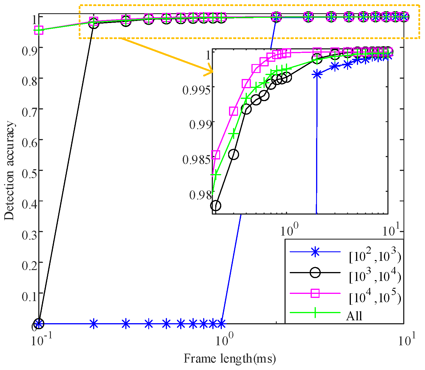
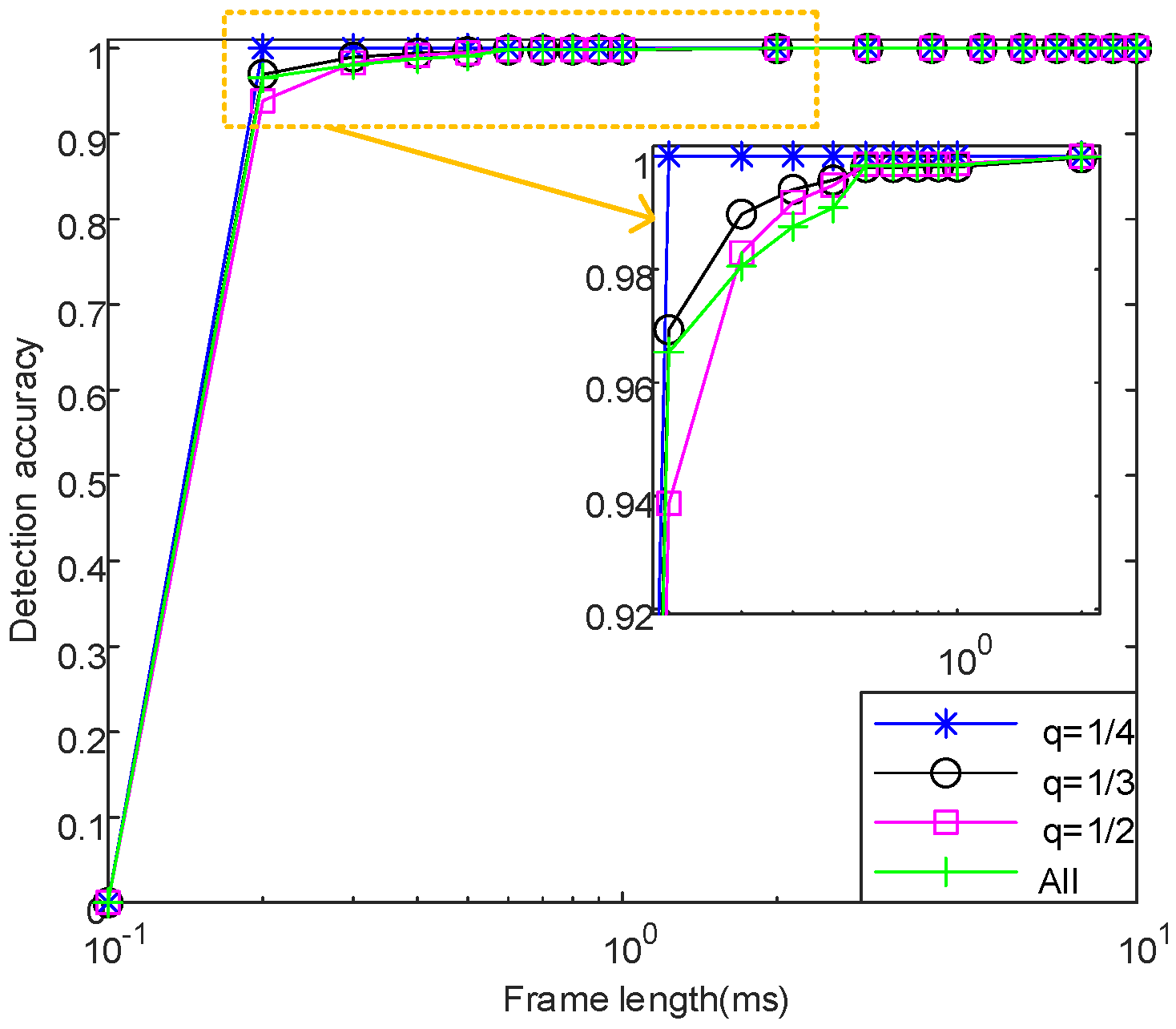
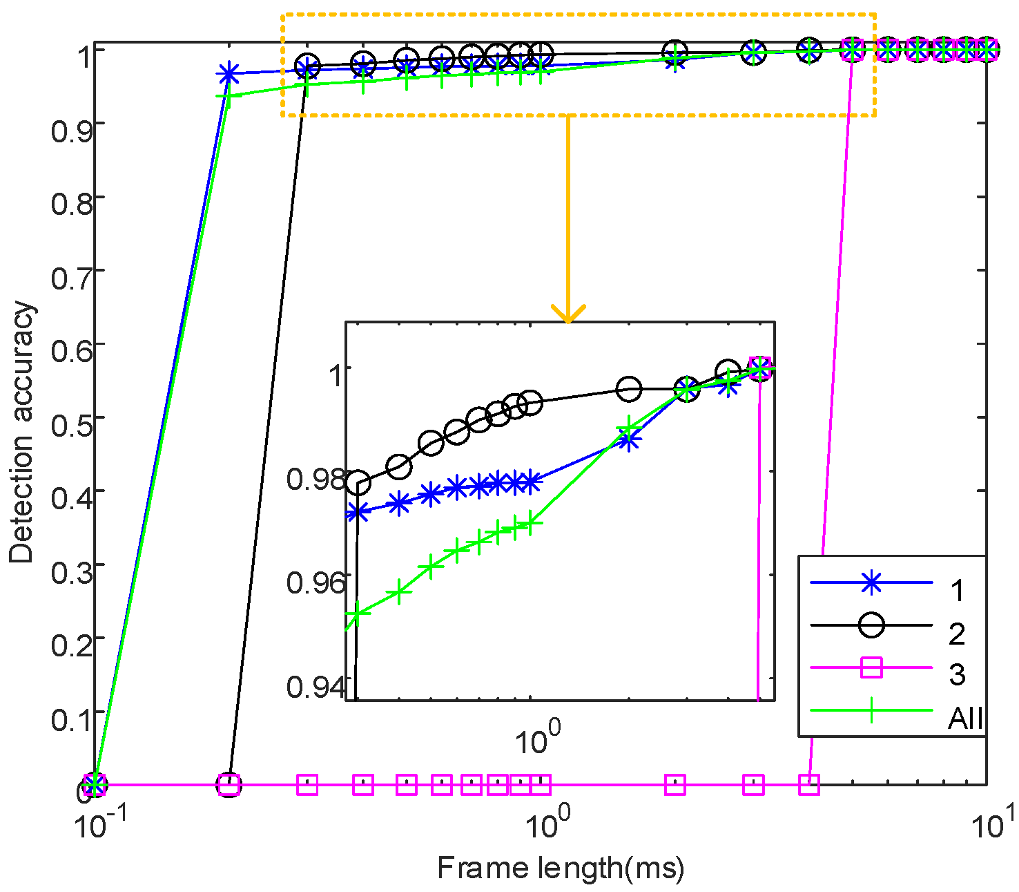
The frame length determines the length of the data sequence processed by the split pulse detection algorithm in a single iteration. Below, the test will be conducted to determine whether the frame length affects the result of the split pulse detection. The range of frame length variation for different pulse flow characteristics is set as [ 0.1 : 0.1 : 0.9 , 1 : 1 : 10 ] ms. The results of comparative experiments using simulation data are shown in Figure 28, Figure 29, Figure 30, Figure 31 and Figure 32. The accuracy of split pulse detection is calculated as the percentage of correctly detected timeframes out of the total number of timeframes. Because the split pulse is randomly generated, it is necessary to set up 100 Monte Carlo simulation experiments, and the average of the detection results generated many times under the same experimental condition is used to ensure the stability of the detection results. Since the split pulse is generated randomly, it is necessary to set 100 Monte Carlo simulation experiments and calculate the mean value of the detection results generated repeatedly under the same experimental conditions to ensure the stability of the detection results.
Figure 28 shows the detection effect with only pulse flow density changes, and ’All’ means that pulse flow density is not distinguished. When the pulse flow density and frame length are both relatively small, it becomes difficult to detect whether the pulse is split. When the pulse flow density is [ 10 2 , 10 3 ) pulse numbers per picosecond, and the frame length T f 1 ms, the detection accuracy is 0. When the pulse flow density is [ 10 3 , 10 4 ) pulse numbers per picosecond and the frame length T f = 0.1 ms, the detection accuracy is 0. It can be seen that the smaller the pulse flow density, the more sensitive the frame length selection. The reason for the above phenomenon is that once the pulse flow density becomes smaller, the pulse flow will become sparse when it arrives. When the frame length is relatively small, it is easy to have an extreme situation in which only one split pulse exists in the frame, so that a single split pulse is misjudged as a complete pulse. In addition, regardless of the pulse flow density in the range, with the increase in frame length, the detection accuracy will gradually increase and exceed 99.9% and then remain unchanged. Comparing the change trend of detection effect of different pulse flow density, it can be seen that the higher the pulse flow density, the higher the detection accuracy. When the frame length is large, the algorithm has an accurate detection effect on different pulse flow densities.
Figure 29 shows the detection effect of only pulse splitting degree changes, and ’All’ indicates that the pulse-splitting degree is not distinguished. If the frame length is relatively small, it is impossible to detect whether the pulse is split. When T f = 0.1 ms, the detection accuracy is 0. This is because when the frame length is relatively small, regardless of the degree of pulse splitting, the single split pulse remaining in the frame may be misjudged as a complete pulse, leading to detection errors. It can be seen that the selection of frame length has similar sensitivity to different degrees of pulse splitting. In addition, as the frame length increases, the detection accuracy gradually increases to 100% and remains constant. Comparing the trend of detection accuracy for different pulse-splitting degrees, it can be observed that the detection effect becomes more significant as the pulse-splitting degree decreases. When the frame length is large, the algorithm has a reliable detection effect for various degrees of pulse splitting.
Figure 30 shows the detection effect with only pulse staggering degree changes, and ’All’ indicates that the pulse-staggering degree is not distinguished. If the frame length is small, the split pulse cannot be detected. When R N = 1 and T f = 0.1 ms, R N = 2 and T f 0.2 ms, and R N = 3 and T f 4 ms, the detection accuracy is 0. It can be observed that as the pulse staggering degree increases, the requirement for frame length selection becomes more stringent. The above phenomenon can be attributed to two reasons. One reason is that when the frame length is reduced to the point where it no longer meets the agreed degree of pulse interleaving within a single timeframe, the calculation detection accuracy rate becomes meaningless. Therefore, the detection accuracy rate is set to 0. The second reason is that a frame length that is too small will cause the algorithm to mistake the only split pulse in a single timeframe for a complete pulse, resulting in detection errors. In addition, regardless of the degree of pulse staggering, the detection accuracy rate gradually increases to 100% as the frame length increases. It can be seen that when the frame length selection meets the detection requirements for pulse staggering degree within a single timeframe, the algorithm demonstrates a remarkable detection effect across various pulse staggering degrees.
Figure 31 shows the detection effect of only PRI modulation complexity changes, and ’All’ indicates that PRI modulation complexity is not distinguished. When T f = 0.1 ms, the detection accuracy of all PRI modulation types is 0, and the reason for this phenomenon is consistent with Figure 29. It can be seen that selecting a frame length that is too small for different PRI modulation complexities will result in detection errors. In addition, as the frame length increases, the detection accuracy gradually increases and exceeds 99.8%. By comparing the change trend of detection accuracy for different PRI modulation complexities, it can be observed that the detection accuracy is higher for simpler PRI modulation types. Therefore, when the frame length is large, the algorithm has a reliable detection effect on different PRI modulation types.
Figure 32 shows the detection effect of the comprehensive change in pulse flow characteristics. According to the trend of detection effect, as the frame length decreases, there is a higher likelihood of misjudging a single split pulse within the frame as a complete pulse, leading to a worse detection effect. Conversely, a longer frame length results in a better detection effect.
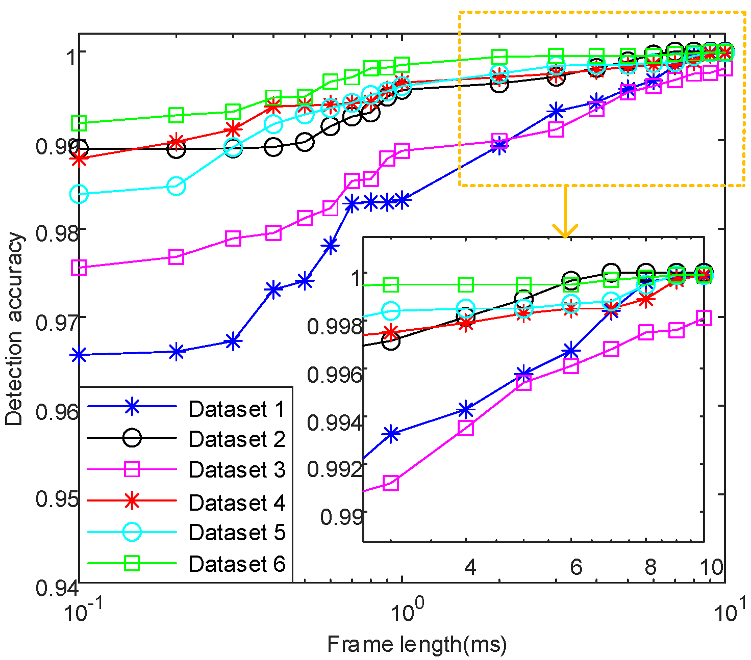
Figure 33 shows the changing trend of the detection effect for the selected six groups of experimental datasets. It can be observed that the change pattern of the experimental dataset is similar to that of the simulation dataset. The detection accuracy rate gradually improves and consistently exceeds 96% as the frame length increases, which confirms that the algorithm can reliably produce accurate results on the experimental dataset. To summarize, as long as the frame length is reasonable, the split pulse detection effect remains reliable regardless of any changes in the pulse flow characteristics. In engineering applications, the frame length is generally not less than 5 ms.

4.3.3. Split Pulse Detection Threshold

Table 8 presents the simulation data results for the mean p m e a n , maximum p m a x , minimum p m i n and the difference between the maximum and minimum values Δ p of the split pulse detection accuracy for different pulse flow characteristics. The results are obtained from 100 Monte Carlo simulation experiments. It can be seen that 99.55% of the minimum detection accuracy of p m e a n comes from the fixed PRI modulation type, while 99.96% of the minimum detection accuracy of p m a x , 95.55% of the minimum detection accuracy of p m i n , and 4.41% of the peak value of Δ p all derive from the comprehensive pulse flow characteristics. The results show that when the split pulse detection algorithm is applied to the changing complex electromagnetic environment, compared with the changing single pulse flow characteristics, the detection accuracy and the stability of the algorithm are slightly worse.
Then, the detection algorithm is applied to the experimental data, as shown in Table 9. The detection accuracy p is maintained above 95.68%, which verifies the accuracy and stability of the empirical formula for the split pulse detection threshold.

5. Conclusions

This paper solves the problem of split pulse detection in a radar pulse stream, and it proposes a method of split pulse modeling and detection. Firstly, the generation mechanism of split pulse is analyzed, and the theory of split site is proposed to describe different splitting modes. Then, the split pulse signal model and the statistical model of split pulse number based on geometric distribution are constructed, respectively, to construct the simulation data of a split pulse under different characteristics. Furthermore, in order to avoid a large number of threshold searches during pulse splitting detection, an empirical formula of the pulse-splitting detection threshold based on the convergence degree in a time domain is given to quickly determine whether there is a split pulse in the radar pulse stream.
Experiments demonstrate the following:
  • Under a significance level of 0.05, it was verified that the split pulse number of the selected measured radar pulse stream follows a geometric distribution.
  • When the window length is greater than 1, the defined time-domain convergence degree is effective and can produce valid results for split pulse detection.
  • Keeping other conditions constant, when only the pulse flow density varies, a higher pulse flow density leads to a higher detection accuracy. As the frame length increases, the detection accuracy gradually increases and exceeds 99.9%, remaining stable thereafter.
Keeping other conditions constant, when only the pulse-splitting degree changes, a smaller pulse-splitting degree results in a more significant detection effect. As the frame length increases, the detection accuracy gradually increases, reaching 100% and remaining constant.
Keeping other conditions constant, when only the pulse-staggering degree changes, a higher pulse-staggering degree requires selecting a larger frame length to ensure an effective detection effect. As the frame length increases, the detection accuracy gradually rises to 100% and remains constant.
Keeping other conditions constant, when only the PRI modulation cmplexity changes, simpler PRI modulation types lead to higher detection accuracy. As the frame length increases, the detection accuracy gradually increases, exceeding 99.8%.
When the characteristics of the pulse stream vary in a comprehensive manner, the detection performance gradually increases with the increase in frame length, exceeding 99%.
4.
Using the detection algorithm for both simulation and experimental data, the obtained detection accuracy remains above 95.68%, confirming the accuracy and stability of the empirical formula for split pulse detection threshold.
In summary, the constructed simulation data accurately reproduce real-world scenarios. The split pulse detection method is effective for both simulation and experimental data, validating the correctness of the modeling and the stability of the detection method.
Limitations:
The pulse-splitting model proposed in this paper only considers the pulse splitting caused by radar reconnaissance equipment without taking into account environmental factors such as multipath effects and colored noise. When the timeframe length is set too small, the pulse-splitting detection method proposed in this paper becomes ineffective.

Author Contributions

Conceptualization, R.G.; methodology, R.G.; software MATLAB 2019b, R.G.; validation, R.G. and W.L.; formal analysis, Y.-Y.D. and D.B.; investigation, R.G.; resources, C.D.; data curation, R.G.; writing—original draft preparation, R.G.; writing—review and editing, Y.-Y.D. and D.B.; visualization, Z.L.; supervision, L.Z.; project administration, C.D.; funding acquisition, Y.-Y.D. All authors have read and agreed to the published version of the manuscript.

Funding

This research was funded by the National Natural Science Foundation of China, grant number 61901332.

Data Availability Statement

The datasets analyzed during the current study are available from the corresponding author on reasonable request. The data are not publicly available due to [data available on request due to privacy].

Conflicts of Interest

The authors declare no conflicts of interest.

References

  1. Dandan, D. Research on Signal Detection and Sorting Technology in Passive Detection Equipment. Master’s Thesis, Harbin Engineering University, Harbin, China, 2018. [Google Scholar]
  2. Li, C.; Wang, W.; Wang, X.-S. Pulse Detection Algorithm based on box Differential Filter. Syst. Eng. Electron. 2013, 35, 1615. [Google Scholar]
  3. D’amico, A.A.; Mengali, U.; Taponecco, L. Energy-Based TOA Estimation. IEEE Trans. Wirel. Commun. 2008, 7, 838–847. [Google Scholar] [CrossRef]
  4. Xi, Y.; Liu, Y.; Jing, S. Real-time detection algorithm and performance analysis of electronic reconnaissance signal. J. Nanjing Univ. Aeronaut. Astronaut. 2001, 3, 277–281. [Google Scholar]
  5. Simin, Z.; Deguo, Z.; Bin, T. A wideband pulse detection algorithm based on autocorrelation. In Proceedings of the 2009 9th International Conference on Electronic Measurement & Instruments, Beijing, China, 16–19 August 2009; pp. 4-287–4-289. [Google Scholar] [CrossRef]
  6. Liu, X.; Fan, X.; Su, S. Adaptive pulse edge detection algorithm based on short-time Fourier transforms and difference of box filter. J. Appl. Remote. Sens. 2019, 13, 024502. [Google Scholar] [CrossRef]
  7. Luo, W. Pulse Signal Detection Method Based on Double Extended Duffing Oscillator. J. Syst. Simul. 2019, 31, 1416–1420. [Google Scholar] [CrossRef]
  8. Cao, C.; Yu, Y. Analysis of influencing factors of Pulse Detection. Electron. Inf. Countermeas. Technol. 2020, 35, 46. [Google Scholar]
  9. Gong, S.X.; Wei, X.Z.; Li, X. Review of Wideband Digital Channelized Receivers. Acta Electron. Sin. 2013, 41, 949. [Google Scholar]
  10. Li, Q.J. On the Impedance Mismatch Channel Model of G.fast Digital Subscriber Line. Acta Electron. Sin. 2020, 48, 403. [Google Scholar]
  11. Jiang, L.B.; Zhou, X.L.; Che, L. Few-Shot Learning for Human Motion Recognition Based on Carrier-Free UWB Radar. Acta Electron. Sin. 2020, 48, 602. [Google Scholar]
  12. Zou, G. Design and Implementation of Ultra Wideband Radar Signal Reconnaissance and Acquisition Processor. Master’s Thesis, Beijing Institute of Technology, Beijing, China, 2015. [Google Scholar]
  13. Liu, Y. Signal Parameter Measurement Method and DSP Software Implementation of Spaceborne Ultra-Wideband Radar. Master’s Thesis, Beijing Institute of Technology, Beijing, China, 2016. [Google Scholar]
  14. Jiang, H.; Guo, Y.; Zhao, F. Split pulse combination in UWB radar signal reconnaissance system. In Proceedings of the 2017 10th International Congress on Image and Signal Processing, BioMedical Engineering and Informatics (CISP-BMEI), Shanghai, China, 14–16 October 2017; pp. 1–5. [Google Scholar] [CrossRef]
  15. Tang, L. Channeled Wideband Radar Signal Detection and FPGA Implementation. Master’s Thesis, Nanjing University of Science and Technology, Nanjing, China, 2022. [Google Scholar]
  16. Wang, C.; Sun, L.; Wang, X. Based on radar intra-pulse chirp pulse splitting signal separation and parameter estimation. J. Signal Process. 2023, 39, 1222. [Google Scholar] [CrossRef]
  17. Wu, Z.; Xia, H. Research on the false signal processing method caused by channelization. Technol. Electron. 2021, 34, 25–30. [Google Scholar] [CrossRef]
  18. Gui, Y.; Wang, B. Research on digital channelization and false signal. Mod. Radar 2016, 38, 23–27. [Google Scholar] [CrossRef]
  19. Cirrone, G.; Donadio, S.; Guatelli, S.; Mantero, A.; Mascialino, B.; Parlati, S.; Pia, M.; Pfeiffer, A.; Ribon, A.; Viarengo, P. A goodness-of-fit statistical toolkit. IEEE Trans. Nucl. Sci. 2004, 51, 2056–2063. [Google Scholar] [CrossRef]
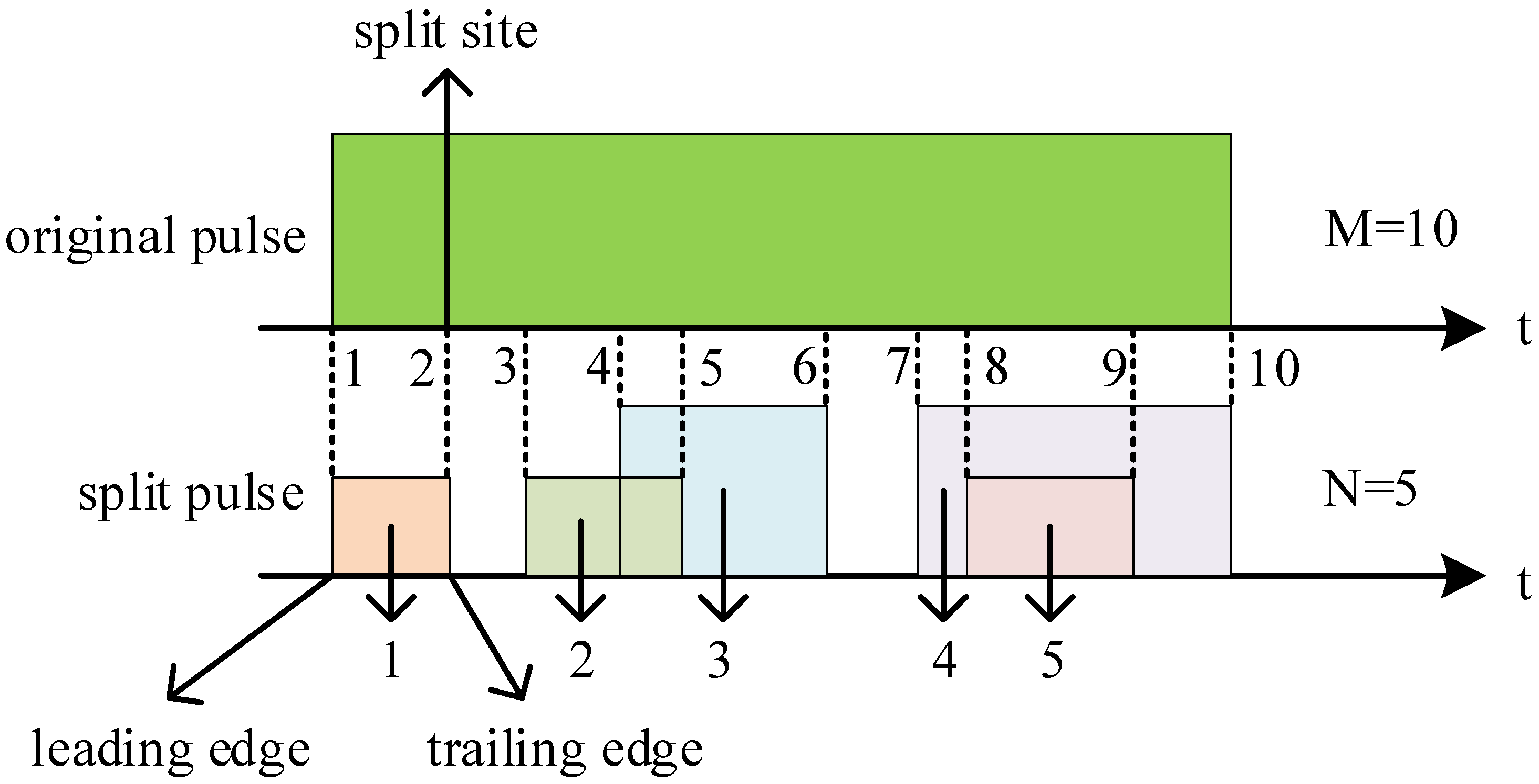
Figure 1. The schematic of pulse split site.
Remotesensing 16 00521 g001
Figure 2. The schematic of cross-channel signal split.
Remotesensing 16 00521 g002
Figure 3. The simulation diagram of cross-channel signal split.
Remotesensing 16 00521 g003
Figure 4. The overlapping split sites of the split pulses.
Remotesensing 16 00521 g004
Figure 5. The schematic of rabbit ear effect.
Remotesensing 16 00521 g005
Figure 6. The simulation diagram of rabbit ear effect.
Remotesensing 16 00521 g006
Figure 7. The independent split sites of the split pulses.
Remotesensing 16 00521 g007
Figure 8. The schematic of transition band repeated signal.
Remotesensing 16 00521 g008
Figure 9. The simulation diagram of transition band repeated signal.
Remotesensing 16 00521 g009
Figure 10. The mutually contained split sites of the split pulses.
Remotesensing 16 00521 g010
Figure 11. Geometric distribution law of splitting pulse number.
Remotesensing 16 00521 g011
Figure 12. Average number of split pulses with different PWs.
Remotesensing 16 00521 g012
Figure 13. Average number of split pulses of different PA.
Remotesensing 16 00521 g013
Figure 14. Flowchart of split pulse detection.
Remotesensing 16 00521 g014
Figure 15. FSTD.
Figure 15. FSTD.
Remotesensing 16 00521 g015
Figure 16. IFSTD.
Figure 16. IFSTD.
Remotesensing 16 00521 g016
Figure 17. The DC of independent split pulses.
Remotesensing 16 00521 g017
Figure 18. The DC of dependent split pulses.
Remotesensing 16 00521 g018
Figure 19. The DC of only one pulse in a timeframe.
Remotesensing 16 00521 g019
Figure 20. Pulse stream with a lower TCD (absence of split pulses).
Remotesensing 16 00521 g020
Figure 21. Pulse stream with a higher TCD (presence of split pulses).
Remotesensing 16 00521 g021
Figure 22. Pulse stream with a higher TCD (presence of overlapping pulses).
Remotesensing 16 00521 g022
Figure 23. Missing pulse length.
Remotesensing 16 00521 g023
Figure 24. Split pulse merging process.
Remotesensing 16 00521 g024
Figure 25. Comparison of experimental data distribution law and geometric distribution law.
Remotesensing 16 00521 g025
Figure 26. The existence of split pulses.
Remotesensing 16 00521 g026
Figure 27. The nonexistence of split pulses.
Remotesensing 16 00521 g027
Figure 28. Pulse flow density.
Remotesensing 16 00521 g028
Figure 29. Pulse-splitting degree.
Remotesensing 16 00521 g029
Figure 30. Pulse-staggering degree.
Remotesensing 16 00521 g030
Figure 31. PRI modulation complexity.
Remotesensing 16 00521 g031
Figure 32. Multifactor.
Remotesensing 16 00521 g032
Figure 33. Experimental data.
Remotesensing 16 00521 g033
Table 1. Advantages and disadvantages of existing radar pulse-splitting methods.
Existing Radar
Pulse-Splitting Methods
AdvantagesDisadvantages
[2,3,4,5,6,7]They have studied radar pulse detection algorithms.They have not studied radar pulse-splitting detection algorithms.
[17,18]They have conducted mechanistic studies on the three scenarios of pulse splitting.They have not mathematically modeled the phenomenon of pulse splitting.
[12,13,14,15]They have described the merging conditions and methods of split pulses.They have not studied the statistical regularities of split pulse numbers.
[16]The proposed pulse splitting model only considers mutually independent split pulses.The model does not consider other splitting scenarios, and there has been no investigation into the statistical regularities of split pulse numbers.
Table 2. The maximum number of split pulses required to form a complete pulse.
p1/51/41/31/22/33/44/5
l + 1 33262012876
Table 3. Reference label generation method.
Timeframe FeatureLabel
There exists at least one original PDW with a split pulse number greater than 1.1
The split pulse number corresponding to the original PDW is at most 1.0
No pulse is received.−1
Table 4. Discriminative labels generated by the algorithm.
The Convergence Derivative Matrices k τ and k DC Label
All zero matrices0
Not all zero matrices1
No pulse is received−1
Table 5. Simulation data.
Radar Numberf/MHz τ / μ s PA /dB PRI / μ s
A 4930 5005 20 ± 0.1 86 70 60 ± 0.1
B 4000 4600 15 ± 0.1 94 82 350 ± 0.2
C 4875 4925 30 ± 0.1 95 81 2008 ± 0.3
D 5329 5331 6 ± 0.1 95 78 543 ± 0.2
E 6350 6860 14 ± 0.1 92 87 250 ± 0.2
F 6100 6200 29 ± 0.1 93 90 1850 ± 0.3
G 5494 5525 79 ± 0.1 87 76 2890 ± 0.3
H (fixed PRI) 5494 5525 79 ± 0.1 87 76 2890 ± 0.3
I (staggered PRI)Pulse 1 5158 5168 15 ± 0.1 72 57 1947 ± 0.3
Pulse 2 6178 6184 40 ± 0.1 67 55 454 ± 0.2
J (group staggered PRI)Pulse 3 5900 5950 11 ± 0.1 85 75 511 ± 0.2
Pulses 4,5 6940 6990 31 ± 0.1 83 72 1007 ± 0.3
Pulses 6,7 4050 4100 63 ± 0.1 87 73 1040 ± 0.3
Pulse 8 5140 5220 127 ± 0.1 83 72 2063 ± 0.3
L
(staggered PRI,
q = 1/3)
Pulse 9 5190 6000 26 ± 0.1 74 67 600 ± 0.2
Pulse 10 7360 7610 32 ± 0.1 77 65 960 ± 0.2
Pulse 11 6560 6700 26 ± 0.1 79 68 1550 ± 0.3
M
(group staggered PRI,
q = 1/2)
Pulse 12,13 5560 5890 17 ± 0.1 86 79 530 ± 0.2
Pulses 14,15,16 6390 6600 22 ± 0.1 89 73 850 ± 0.2
Pulses 17 5230 5580 55 ± 0.1 86 75 1350 ± 0.3
Table 6. Experimental data.
Dataset Numberf/MHz τ / μ s PA /dB PRI / μ s
1 (fixed PRI) 5000 5490 1 ± 0.1 89 83 100 ± 0.2
2 (fixed PRI) 5900 6000 10 ± 0.1 93 73 150 ± 0.2
3 (staggered PRI) 6650 6700 13 ± 0.1 88 79 (50, 300) ± 0.2
4 (staggered PRI) 7700 7800 15 ± 0.1 85 78 (100, 400) ± 0.2
5 (group staggered PRI) 6500 6700 22 ± 0.1 89 80 (60,60,110,110,160) ± 0.2
6 (group staggered PRI) 5300 5600 35 ± 0.1 84 76 (70,70,115,115,130) ± 0.2
7 (fixed PRI) 7300 7900 50 ± 0.1 89 77 500 ± 0.2
8 (fixed PRI) 6600 7100 200 ± 0.1 93 77 1000 ± 0.2
Table 7. Statistical table of split pulse numbers corresponding to the original pulses.
i12345
f i 21902860096282422189314209
f i / E 60.72%16.66%7.83%6.07%3.94%
i 678910
f i 8010390719621023672
f i / E 2.22%1.08%0.54%0.28%0.19%
i 1112131415
f i 518391303243237
f i / E 0.14%0.11%0.08%0.07%0.07%
Table 8. Under different pulse flow characteristics, the accuracy of split pulse detection is used to verify the validity of the empirical formula for determining the split pulse detection threshold.
Pulse Flow CharacteristicPulse Flow Density
Experiment condition [ 10 2 , 10 3 ) [ 10 3 , 10 4 ) [ 10 4 , 10 5 ) All
p m e a n 99.86%100%100%99.96%
p m a x 100%100%100%100%
p m i n 99.5%99.87%99.82%99.85%
Δ p 0.5%0.13%0.18%0.15%
Pulse flow characteristicPulse splitting degree
Experiment condition 1 / 4 1 / 3 1 / 2 All
p m e a n 100%100%100%100%
p m a x 100%100%100%100%
p m i n 100%100%100%100%
Δ p 0%0%0%0%
Pulse flow characteristicPulse staggering degree
Experiment condition 1 2 3 All
p m e a n 100%100%100%100%
p m a x 100%100%100%100%
p m i n 100%100%100%100%
Δ p 0%0%0%0%
Pulse flow characteristicPRI modulation complexity
Experiment conditionFixed PRIStaggered PRIGroup staggered PRIAll
p m e a n 99.55%99.8%99.84%99.73%
p m a x 100%100%100%100%
p m i n 96.98%98.59%99.12%98.83%
Δ p 3.02%1.41%0.88%1.17%
Pulse flow characteristicComprehensive characteristics
p m e a n 99.61%
p m a x 99.96%
p m i n 95.55%
Δ p 4.41%
Table 9. Under the experimental dataset, the accuracy of split pulse detection is used to verify the rationality of the empirical formula of split pulse detection threshold.
Dataset Number123456
p95.68%99.54%98.11%98.98%98.81%99.48%
Disclaimer/Publisher’s Note: The statements, opinions and data contained in all publications are solely those of the individual author(s) and contributor(s) and not of MDPI and/or the editor(s). MDPI and/or the editor(s) disclaim responsibility for any injury to people or property resulting from any ideas, methods, instructions or products referred to in the content.