
Water Footprint of Cereals by Remote Sensing in Kairouan Plain (Tunisia)

 , , ,
, , ,  ,
,  and
and
Abstract
1. Introduction
2. Materials and Methods
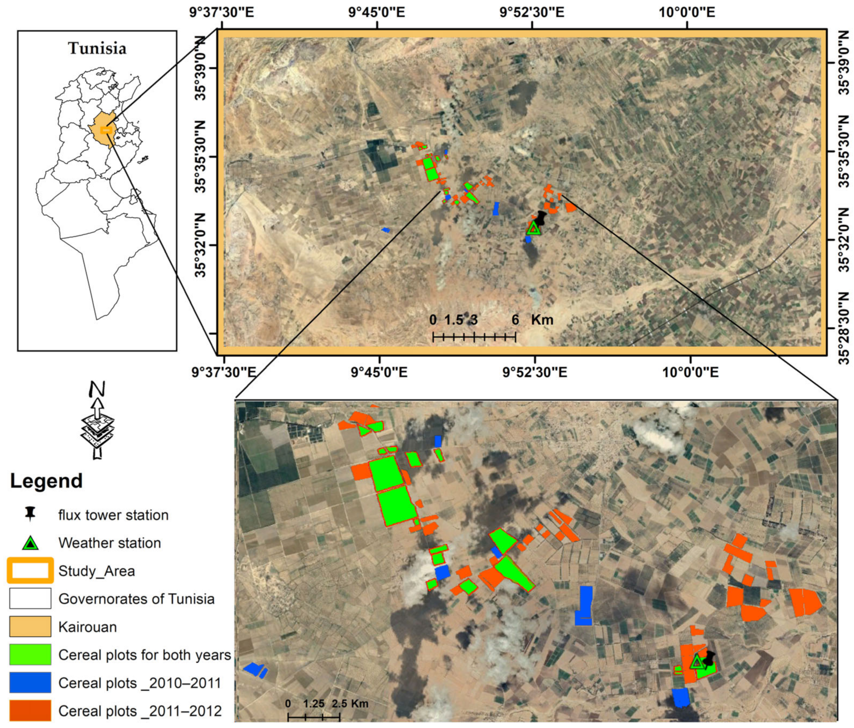
2.1. Study Area
2.2. Satellite and Ground Data
2.2.1. Satellite Data
2.2.2. Ground Data
2.3. Water Footprint Background
- WF:
- water footprint (m3/kg).
- CWU:
- crop water use (m3/ha).
- Y:
- yield (kg).
- ET:
- evapotranspiration determined for each period from day 1 to lgp (length of growing period) (mm/day).
- R:
- actual rainfall (mm/day).
- a:
- empirical parameter representing the crop saturation per unit foliage area (~0.28 for most crops).
2.4. WF Components by Earth Observation
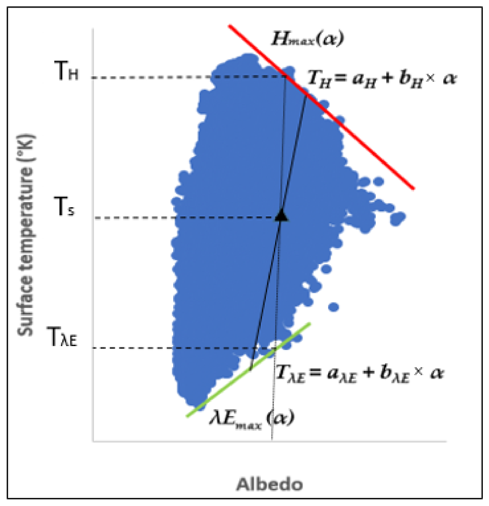
2.4.1. Evapotranspiration by S-SEBI Model
- Rn:
- net radiation (W × m−2).
- G0:
- soil heat flux (W × m−2).
- H:
- sensible heat flux (W × m−2).
- λE:
- latent heat flux (W × m−2).
- α:
- surface albedo [-].
- :
- the atmospheric transmittance (-) is a function of θs, where: θs is the solar zenith angle described earlier (degree) after [46].
- :
- exoatmospherical incoming solar radiation (W × m−2).
- S:
- is the exa-atmospheric incident solar radiation (solar constant = 1395 (W.m−2)).
- λ:
- latitude (degree).
- δ:
- declination of the Sun.
- h:
- hour angle (h = (12-h) × 15) (degree).
- :
- Stefan–Boltzmann constant (5.67 × 10⁻⁸ W × m−2 × K−4).
- :
- surface emissivity.
- T0:
- surface temperature (°K).
- L↓:
- long-wave incoming radiation. It is measured as per [18] and is equal to 350.75 (W × m−2).
- :
- reflectance (planetary albedo) of 650–670 nm band (red) (-).
- :
- reflectance (planetary albedo) of 841–876 nm band (near infrared) (-).
- :
- interpolated Kc between two image acquisition dates.
2.4.2. Earth Observation-Based Yield Evaluation
3. Results
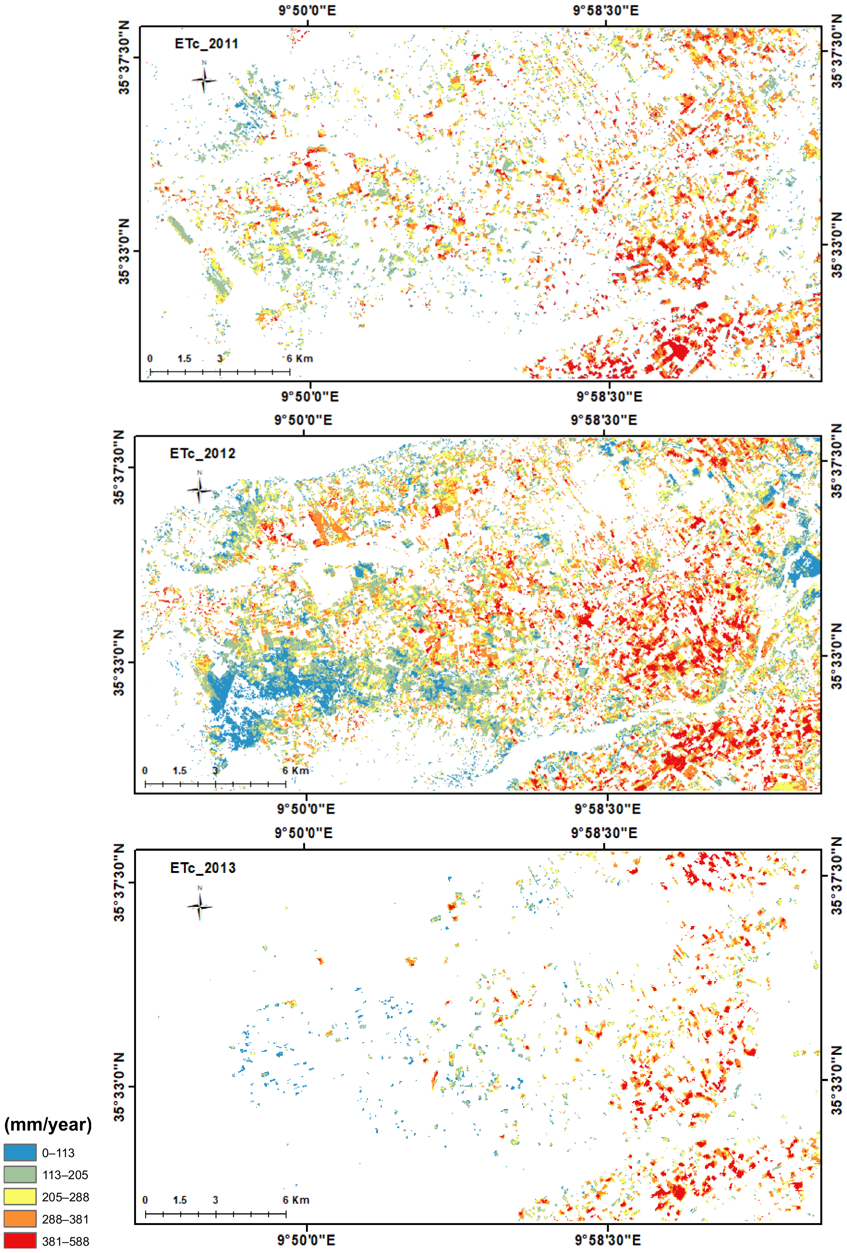
3.1. ETa by S-SEBI and FAO56 Models
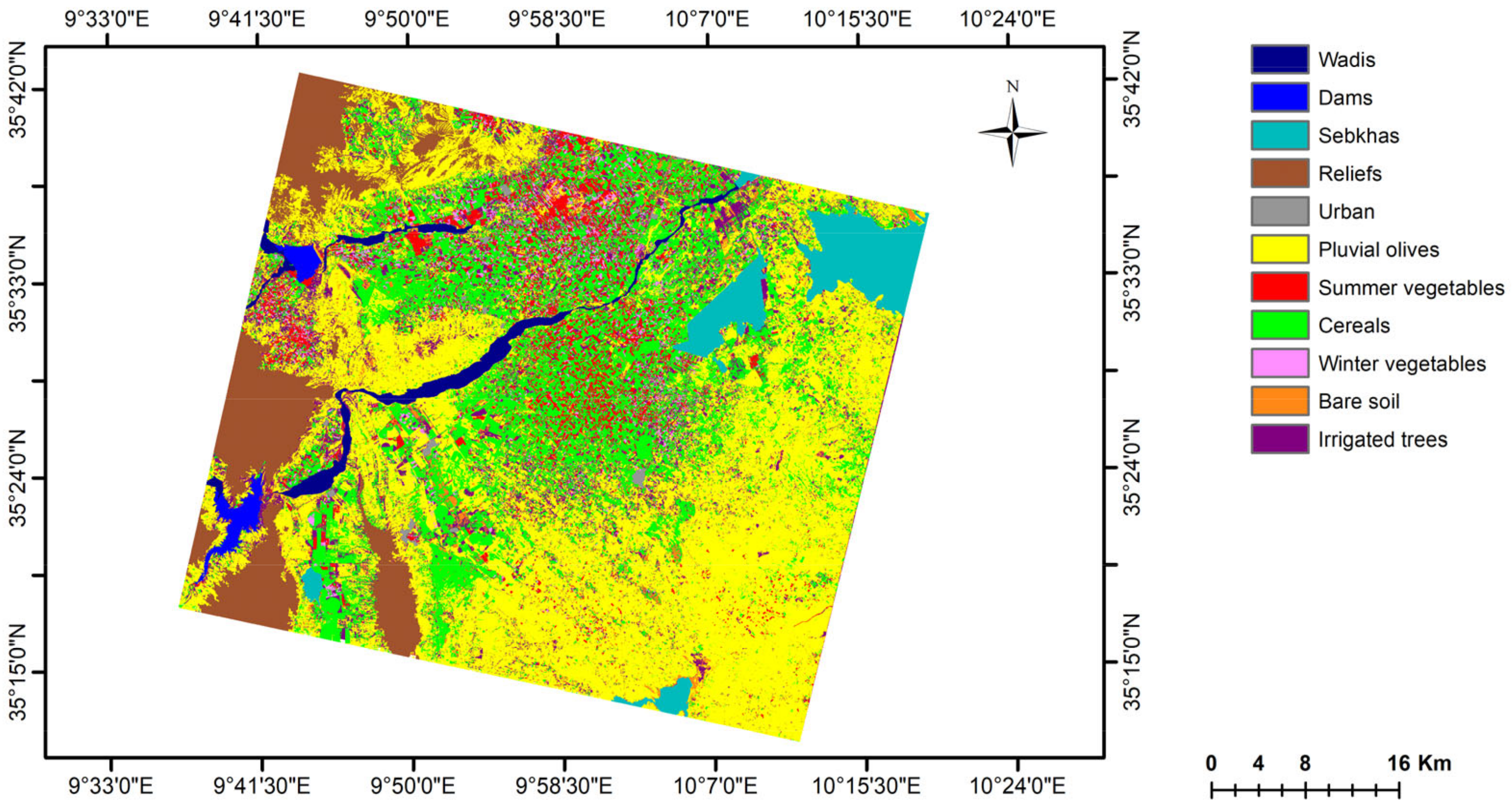
3.2. Yield Mapping
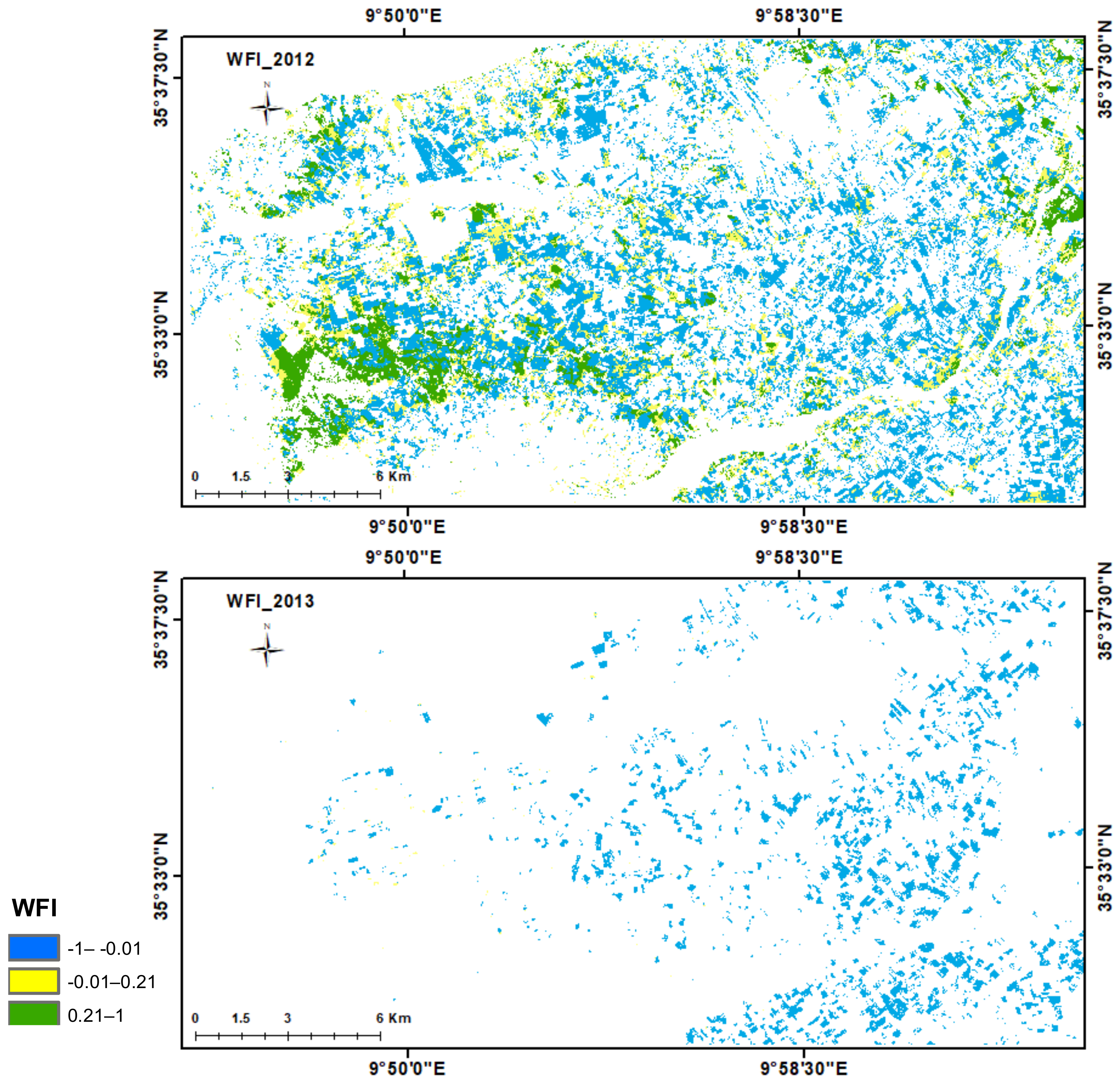
3.3. Water Footprint Mapping
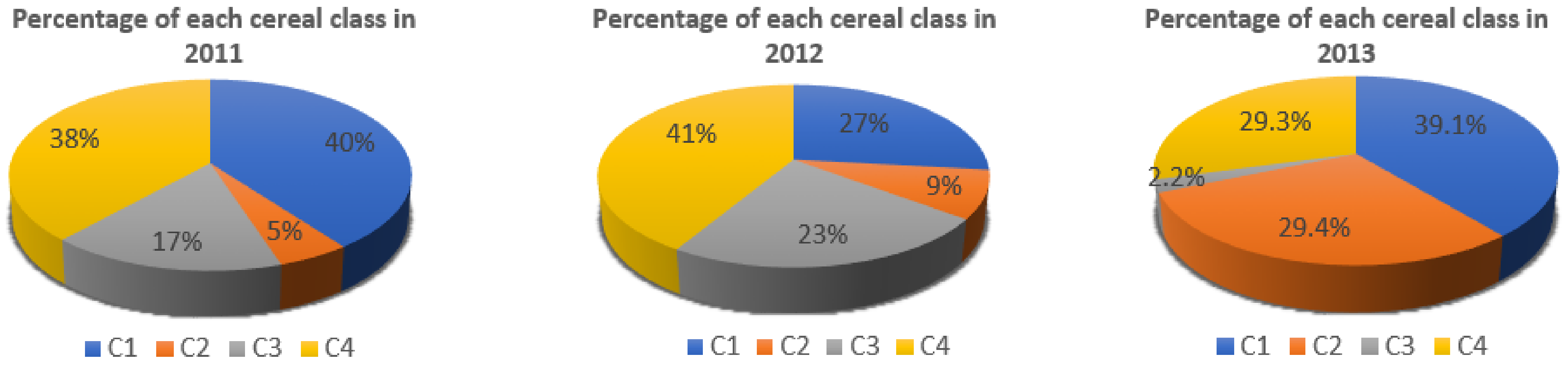
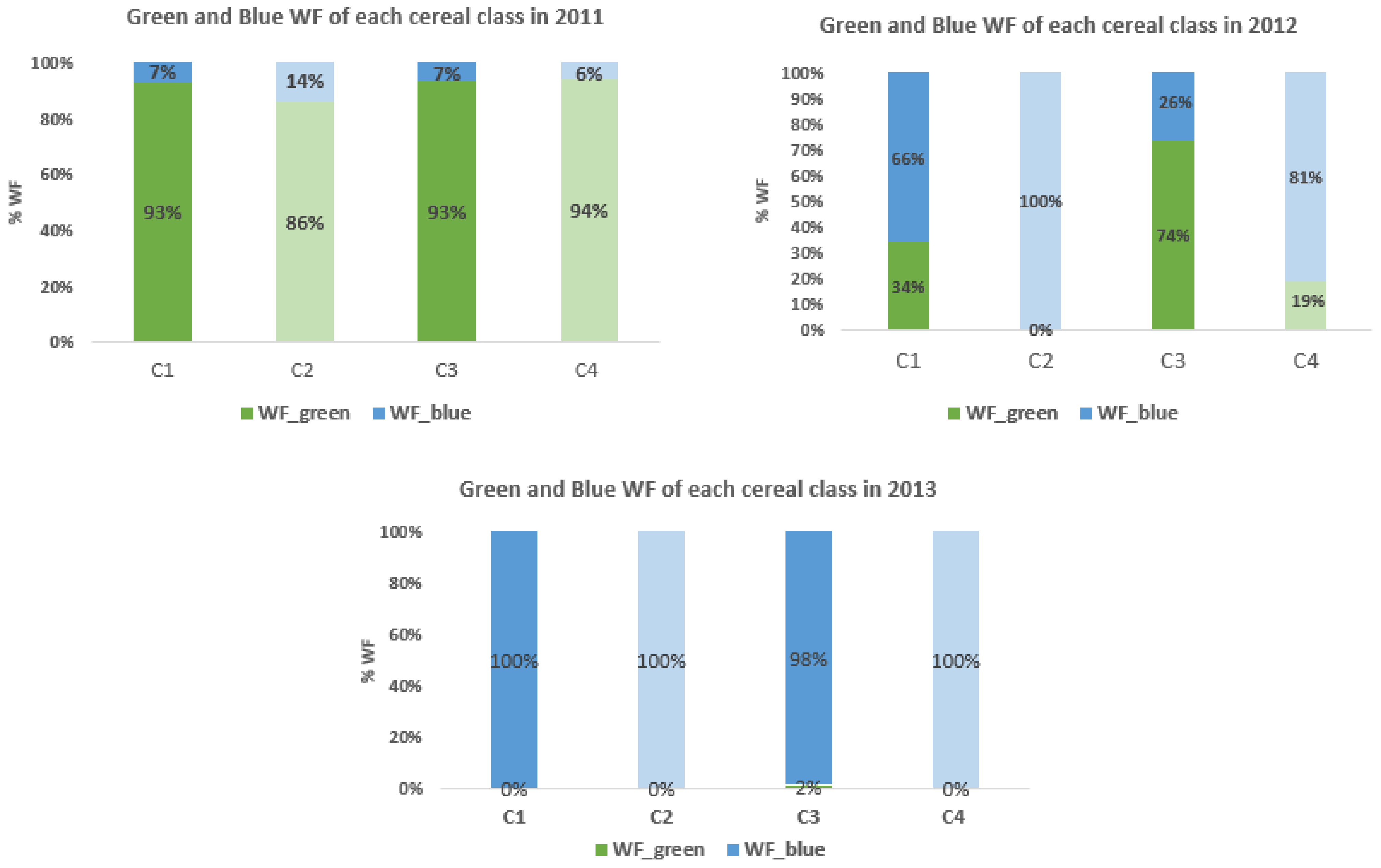
3.3.1. Cereal WF Global Evaluation
3.3.2. Comparing and Assessing Spatiotemporal Variations in WF Cereals
3.3.3. WF–Yield Relationship and Water Management
4. Discussion
5. Conclusions
Author Contributions
Funding
Data Availability Statement
Conflicts of Interest
References
- Falkenmark, M. Shift in Thinking to Address the 21st Century Hunger Gap. Water Resour. Manag. 2007, 21, 3–18. [Google Scholar] [CrossRef]
- Mekonnen, M.M.; Hoekstra, A.Y. The Green, Blue and Grey Water Footprint of Crops and Derived Crop Products. Hydrol. Earth Syst. Sci. Discuss. 2011, 8, 763–809. [Google Scholar] [CrossRef]
- Hoekstra, A.Y.; Chapagain, A.K.; Van Oel, P.R. Progress in Water Footprint Assessment. In Progress in Water Footprint Assessment; MDPI AG: Basel, Switzerland, 2019. [Google Scholar] [CrossRef]
- Schyns, J.F.; Hoekstra, A.Y.; Booij, M.J. Review and Classification of Indicators of Green Water. Hydrol. Earth Syst. Sci. 2015, 19, 4581–4608. [Google Scholar] [CrossRef]
- Hoekstra, A.Y. (Ed.) Virtual water trade. In Proceedings of the International Expert Meeting on Virtual Water Trade, Delft, The Netherlands, 12–13 December 2002; Value of Water Research Report Series No. 12; UNESCO-IHE: Delft, The Netherlands, 2003. [Google Scholar]
- Besbes, M.; Chahed, J.; Hamdane, A. National Water Security: Case Study of an Arid Country: Tunisia; Springer: Berlin/Heidelberg, Germany, 2019; ISBN 9783319754994. [Google Scholar]
- Besbes, M.; Chahed, J.; Hamdane, A. Sécurité Hydrique de la Tunisie; L’Harmattan: Paris, France, 2014. [Google Scholar]
- Chouchane, H.; Krol, M.S.; Hoekstra, A.Y. Virtual Water Trade Patterns in Relation to Environmental and Socioeconomic Factors: A Case Study for Tunisia. Sci. Total Environ. 2018, 613–614, 287–297. [Google Scholar] [CrossRef]
- Chapagain, A.K.; Hoekstra, A.Y. Water Footprints of Nations; Value of Water Research Report Series No. 16; UNESCOIHE: Delft, The Netherlands, 2004; Volume 1–2. [Google Scholar]
- Aldaya, M.M.; Chapagain, A.K.; Hoekstra, A.Y.; Mekonnen, M.M. The Water Footprint Assessment Manual; Setting the Global Standard; Routledge: London, UK, 2011; Volume 31, ISBN 9781849712798. [Google Scholar]
- FAO. Évaluation de L’approvisionnement Alimentaire dans un Contexte de Pénurie d’eau dans le Région NENA; FAO: Rome, Italy, 2018; 165p, ISBN 978-92-5-130826-4. [Google Scholar]
- Latrech; Lasram, A.; M’Nassri, S.; Nciri, R.; Gharbi, W.; Masmoudi, M.M.; Mechlia, N.B. Combining Remote Sensing Data and AquaCrop for Assessement of Yield and Water Productivity of Durum Wheat in Semi-Arid Conditions in Tunisia. Available online: https://swdcc2022.com/wp-content/uploads/2022/08/Session-FAO (accessed on 28 November 2023).
- Zwart, S.J.; Bastiaanssen, W.G.M.; de Fraiture, C.; Molden, D.J. WATPRO: A Remote Sensing Based Model for Mapping Water Productivity of Wheat. Agric. Water Manag. 2010, 97, 1628–1636. [Google Scholar] [CrossRef]
- Allen, R.G.; Pereira, L.S.; Raes, D.; Smith, M. Crop Evapotranspiration-Guidelines for Computing Crop Water Requirements-FAO Irrigation and Drainage Paper 56; Fao: Rome, Italy, 1998; Volume 300, D05109. [Google Scholar]
- Allen, R.G.; Pereira, L.S.; Smith, M.; Raes, D.; Wright, J.L. FAO-56 Dual Crop Coefficient Method for Estimating Evaporation from Soil and Application Extensions; Fao: Rome, Italy, 2005. [Google Scholar]
- Monteith, J.L. Evaporation and environment. Symp. Soc. Exp. Biol. 1965, 19, 205–234. [Google Scholar] [PubMed]
- Calera, A.; Campos, I.; Osann, A.; D’urso, G.; Menenti, M. Remote Sensing for Crop Water Management: From ET Modelling to Services for the End Users. Sensors 2017, 17, 1104. [Google Scholar] [CrossRef]
- Roerink, G.J.; Su, Z.; Menenti, M. S-SEBI: A simple remote sensing algorithm to estimate the surface energy balance. Phys. Chem. Earth Part B Hydrol. Oceans Atmos. 2000, 25, 147–157. [Google Scholar] [CrossRef]
- Li, Z.-L.; Tang, R.; Wan, Z.; Bi, Y.; Zhou, C.; Tang, B.; Yan, G.; Zhang, X. A review of current methodologies for regional evapotranspiration estimation from remotely sensed data. Sensors 2009, 9, 3801–3853. [Google Scholar] [CrossRef]
- Galleguillos, M.; Jacob, F.; Prévot, L.; French, A.; Lagacherie, P. Comparison of two temperature differencing methods to estimate daily evapotranspiration over a Mediterranean vineyard watershed from ASTER data. Remote Sens. Environ. 2011, 115, 1326–1340. [Google Scholar] [CrossRef]
- Acharya, B.; Sharma, V. Comparison of satellite driven surface energy balance models in estimating crop evapotranspiration in semi-arid to arid inter-mountain region. Remote Sens. 2021, 13, 1822. [Google Scholar] [CrossRef]
- Van Ittersum, M.K.; Ewert, F.; Heckelei, T.; Wery, J.; Olsson, J.A.; Andersen, E.; Bezlepkina, I.; Brouwer, F.; Donatelli, M.; Flichman, G.; et al. Integrated assessment of agricultural systems—A component-based framework for the European Union (SEAMLESS). Agric. Syst. 2008, 96, 150–165. [Google Scholar] [CrossRef]
- Balaghi, R.; Tychon, B.; Eerens, H.; Jlibene, M. Empirical Regression Models Using NDVI, Rainfall and Temperature Data for the Early Prediction of Wheat Grain Yields in Morocco. Int. J. Appl. Earth Obs. Geoinf. 2008, 10, 438–452. [Google Scholar] [CrossRef]
- Becker-Reshef, I.; Vermote, E.; Lindeman, M.; Justice, C. A generalized regression-based model for forecasting winter wheat yields in Kansas and Ukraine using MODIS Data. Remote Sens. Environ. 2010, 114, 1312–1323. [Google Scholar] [CrossRef]
- Franch, B.; Vermote, E.F.; Becker-Reshef, I.; Claverie, M.; Huang, J.; Zhang, J.; Justice, C.; Sobrino, J.A. Improving the Timeliness of Winter Wheat Production Forecast in the United States of America, Ukraine and China Using MODIS Data and NCAR Growing Degree Day Information. Remote Sens. Environ. 2015, 161, 131–148. [Google Scholar] [CrossRef]
- Chahbi, A.; Zribi, M.; Lili-Chabaane, Z.; Duchemin, B.; Shabou, M.; Mougenot, B.; Boulet, G. Estimation of the dynamics and yields of cereals in a semi-arid area using remote sensing and the SAFY growth model. Int. J. Remote Sens. 2014, 35, 1004–1028. [Google Scholar] [CrossRef]
- Nougaret, G.; Jenhaoui, Z.; Leduc, C. Ressources en Eau Dans Le Kairouanais: Évolutions des Disponibilités et des Usages DEPUIS 2000 Ans. 2019. Available online: http://www5.funceme.br/arid/wp-content/uploads/2020/05/guide_terrain_Merguellil_04-10-2019-GN-CL.pdf (accessed on 28 November 2023).
- Zribi, M.; Chahbi, A.; Shabou, M.; Lili-Chabaane, Z.; Duchemin, B.; Baghdadi, N.; Amri, R.; Chehbouni, A. Soil Surface Moisture Estimation over a Semi-Arid Region Using ENVISAT ASAR Radar Data for Soil Evaporation Evaluation. Hydrol. Earth Syst. Sci. 2011, 15, 345–358. [Google Scholar] [CrossRef]
- Luca, C.; Michele, M.; Silvia, M. Investigating the Relationship between Land Cover and Vulnerability T0 Climate Change in dar es Salaam; Working Paper April 2013; Sapienza University: Rome, Italy, 2013. [Google Scholar]
- Chavez, P.S. An improved dark-object subtraction technique for atmospheric scattering correction of multispectral data. Remote Sens. Environ. 1988, 24, 459–479. [Google Scholar] [CrossRef]
- Warmerdam, F. The Geospatial Data Abstraction Library. Open Source Approaches Spat. Data Handl. 2008, 2, 87–104. [Google Scholar] [CrossRef]
- Weng, Q.; Lu, D.S.; Schubring, J. Estimation of land surface temperature—Vegetation abundance relationship for urban heat island studies. Remote Sens. Environ. 2004, 89, 467–483. [Google Scholar] [CrossRef]
- Saadi, S.; Simonneaux, V.; Boulet, G.; Raimbault, B.; Mougenot, B.; Fanise, P.; Ayari, H.; Lili-Chabaane, Z. Monitoring Irrigation Consumption Using High Resolution NDVI Image Time Series: Calibration and Validation in the Kairouan Plain (Tunisia). Remote Sens. 2015, 7, 13005–13028. [Google Scholar] [CrossRef]
- Rahman, H.; Dedieu, G. SMAC: A simplified method for the atmospheric correction of satellite measurements in the solar spectrum. Int. J. Remote. Sens. 1994, 15, 123–143. [Google Scholar] [CrossRef]
- Berthelot, B.; Dedieu, G. Correction of Atmospheric Effects for VEGETATION Data. In Physical Measurements and Signatures in Remote Sensing; Guyot, G., Phulpin, T., Eds.; Courchevel: Balkema, France, 1997; pp. 19–25. [Google Scholar]
- Kotchenova, S.Y.; Vermote, E.F.; Matarrese, R.; Klemm, F.J., Jr. Validation of a vector version of the 6S radiative transfer code for atmospheric correction of satellite data. Part I: Path radiance. Appl. Opt. 2006, 45, 6762–6774. [Google Scholar] [CrossRef] [PubMed]
- Tanré, D.; Deroo, C.; Duhaut, P.; Herman, M.; Morcrette, J.J.; Perbos, J.; Deschamps, P.Y. Description of a computer code to simulate the satellite signal in the solar spectrum: The 5S code. Int. J. Remote Sens. 1990, 11, 659–668. [Google Scholar] [CrossRef]
- Caloz, R.; Collet, C. Précis de Télédétection, Volume 3 Traitements Numériques D’images de Télédétection; Presses de l’Université du Québec/AUPELF: Sainte-Foy, QC, Canada, 2001; 386p. [Google Scholar]
- Braden, H. Ein Energiehaushalts- und Verdunstungsmodell for Wasser und Stoffhaushaltsuntersuchungen landwirtschaftlich genutzer Einzugsgebiete. M. Dtsch. Bodenkd. Geselschaft 1985, 42, 294–299. [Google Scholar]
- Moran, M.S.; Clarke, T.R.; Inoue, Y.; Vidal, A. Estimating crop water deficit using the relation between surface-air temperature and spectral vegetation index. Remote Sens. Environ. 1994, 49, 246–263. [Google Scholar] [CrossRef]
- Tucker, J. Red and Photographic Infrared Linear Combinations for Monitoring Vegetation. Remote Sens. Environ. 1979, 150, 127–150. [Google Scholar] [CrossRef]
- Norman, J.M.; Kustas, W.P.; Humes, K.S. Source Approach for Estimating Soil and Vegetation Energy Fluxes in Observations of Directional Radiometric Surface Temperature. Agric. For. Meteorol. 1995, 77, 263–293. [Google Scholar] [CrossRef]
- Chemin, Y. Evapotranspiration of Crops by Remote Sensing Using the Energy Balance Based Algorithms; International Water Management Institute: Pathumithani, Thailand, 2003. [Google Scholar]
- Choudhury, B.J.; Ahmed, N.U.; Idso, S.B.; Reginato, R.J.; Daughtry, C.S.T. Relations between evaporation coefficients and vegetation indices studied by model simulations. Remote Sens. Environ. 1994, 50, 1–17. [Google Scholar] [CrossRef]
- Valor, E.; Caselles, V. Mapping land surface emissivity from NDVI: Application to European, African, and South American areas. Remote Sens. Environ. 1996, 57, 167–184. [Google Scholar] [CrossRef]
- Soudani, K.; Christophe, F.; Et Valérie, L.D. Analyse comparative d’IKONOS, Données SPOT et ETM+ pour l’estimation de l’indice de surface foliaire des conifères et des feuillus tempérés peuplements forestiers. Télédétection L’environnement 2006, 102, 161–175. [Google Scholar]
- Chakroun, H.; Zemni, N.; Benhmid, A.; Dellaly, V.; Slama, F.; Bouksila, F.; Berndtsson, R. Evapotranspiration in Semi-Arid Climate: Remote Sensing vs. Soil Water Simulation. Sensors 2023, 23, 2823. [Google Scholar] [CrossRef]
- Kustas, W.P.; Daughtry, C.S. Estimation of the soil heat flux/net radiation ratio from spectral data. Agric. For. Meteorol. 1990, 49, 205–223. [Google Scholar] [CrossRef]
- Ogée, J.; Lamaud, E.; Brunet, Y.; Berbigier, P.; Bonnefond, J.-M. A long-term study of soil heat flux under a forest canopy. Agric. For. Meteorol. 2001, 106, 173–186. [Google Scholar] [CrossRef]
- Choudhury, B.J. Relationships between vegetation indices, radiation absorption, and net photosynthesis evaluated by a 638 sensitivity analysis. Remote Sens. Environ. 1987, 22, 209–233. [Google Scholar] [CrossRef]
- Santanello, J.A., Jr.; Friedl, M.A. Diurnal covariation in soil heat flux and net radiation. J. Appl. Meteorol. 2003, 42, 851–862. [Google Scholar] [CrossRef]
- Sobrino, J.A.; Gómez, M.; Jiménez-Muñoz, J.C.; Olioso, A. Application of a Simple Algorithm to Estimate Daily Evapotranspiration from NOAA-AVHRR Images for the Iberian Peninsula. Remote Sens. Environ. 2007, 110, 139–148. [Google Scholar] [CrossRef]
- Abdallah, A. Eau Virtuelle et Sécurité Alimentaire en Tunisie: Du Constat à l’Appui au Dévellopement (EVSAT-CAD); Projet de Recherche Developpement: Mograne, Tunisia, 2015. [Google Scholar]
- Chahed, J.; Hamdane, A.; Besbes, M. A comprehensive water balance of Tunisia: Blue water, green water and virtual water. Water Int. 2008, 33, 415–424. [Google Scholar] [CrossRef]
- Ghorbanpour, A.K.; Kisekka, I.; Afshar, A.; Hessels, T.; Taraghi, M.; Hessari, B.; Touri-an, M.J.; Duan, Z. Crop Water Productivity Mapping and Benchmarking Using Re-mote Sensing and Google Earth Engine Cloud Computing. Remote Sens. 2022, 14, 4934. [Google Scholar] [CrossRef]
- Bastiaanssen, W.G.M.; Steduto, P. The Water Productivity Score (WPS) at Global and Regional Level: Methodology and First Results from Remote Sensing Measurements of Wheat, Rice and Maize. Sci. Total Environ. 2017, 575, 595–611. [Google Scholar] [CrossRef]
- Blatchford, M.L.; Karimi, P.; Bastiaanssen, W.; Nouri, H. From Global Goals to Local Gains—A Framework for Crop Water Productivity. ISPRS Int. J. Geo-Inf. 2018, 7, 414. [Google Scholar] [CrossRef]
- Chahed, Y.; Hassan, F.A. 2012 Grain and Feed Update Tunisia. In Global Agricultural Information Network; TS1204; USDA Foreign Agriculture Service: Washington, DC, USA, 2012. [Google Scholar]
- Khlif, M.; Escorihuela, M.J.; Bellakanji, A.C.; Paolini, G.; Kassouk, Z.; Chabaane, Z.L. Multi-Year Cereal Crop Classification Model Using Sentinel 2 and 3 Landsat 7–8 Data. Agriculture 2023, 13, 1633. [Google Scholar] [CrossRef]
- Bousbih, S.; Zribi, M.; Lili-Chabaane, Z.; Baghdadi, N.; El Hajj, M.; Gao, Q.; Mougenot, B. Potential of Sentinel-1 Radar Data for the Assessment of Soil and Cereal Cover Parameters. Sensors 2017, 17, 2617. [Google Scholar] [CrossRef]
- Chouchane, H. Economic Allocation of Water to Crops in International Context: A National and Global Perspective. Ph.D. Thesis, University of Twente, Enschede, The Netherlands, 2019. [Google Scholar]


| Model | Earth Observation | Ground and Auxiliary Data | Process | WF Component |
|---|---|---|---|---|
| S-SEBI | Landsat 7-ETM+ Landsat 8-OLI B2 to B7: 30 m res B10 to B11: 100 m res -LST, Albedo, NDVI, ε (2010–2013) | __ | Daily: -Rn -Evaporative fraction Ʌ -Fluxes: H, G0, λE | Yearly cumulative ETg/b |
| FAO-56 Single crop coefficient | __ | -Air temperature -Air humidity -Solar radiation -Rainfall -Pressure | ET0 (Penman–Monteith, 1965) | ETg/b_FAO56 [36] |
| Yield | SPOT 5 NDVI | -Training site -Yield (82 plots) | -LAI (regression) -Classification (algorithm decision tree) | LAI, land use, yield [29] |
| Rn (W × m−2) | G0 (W × m−2) | H (W × m−2) | λE (W × m−2) | Ʌ (-) | ETa (mm/Day) | |
|---|---|---|---|---|---|---|
| RMSE | 110.96 | 68.28 | 100.87 | 33.35 | 0.18 | 0.45 |
| R2 | 0.54 | 0.09 | 0.05 | 0.85 | 0.51 | 0.82 |
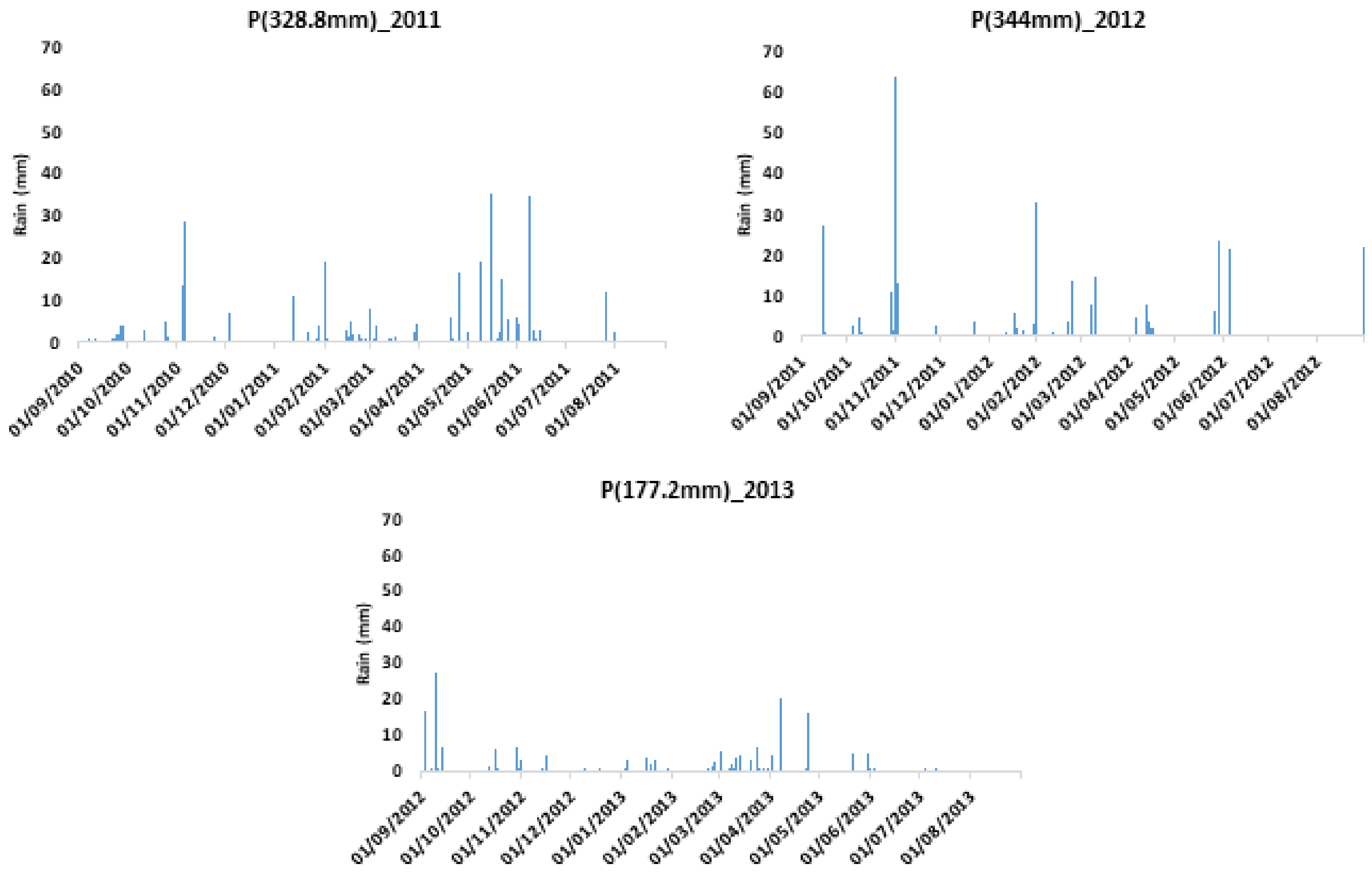
| Year | Rain (mm/year) | Study Area (km2) | Cereal Area (km2) | % Area Cereals | Production (Tons) | Green Water (106 m3/year) | Blue Water (106 m3/year) | Average Green WF (m3/kg) | Average Blue WF (m3/kg) | Total Average WF (m3/kg) |
|---|---|---|---|---|---|---|---|---|---|---|
| 2010–2011 | 328.8 | 444 | 72.48 | 16 | 20,996 | 7.6 | 4.60 | 0.67 (Ϭ = 1.01) | 0.41 (Ϭ = 1.09) | 1.08 |
| 2011–2012 | 344 | 444 | 156.68 | 35 | 40,304 | 13.82 | 18.41 | 0.47 (Ϭ = 0.63) | 0.61 (Ϭ = 1.30) | 1.08 |
| 2012–2013 | 177.2 | 444 | 25.48 | 6 | 8054 | 1.02 | 6.60 | 0.17 (Ϭ = 0.38) | 1.04 (Ϭ = 1.72) | 1.22 |
| 2010–2011 | 2011–2012 | |||
|---|---|---|---|---|
| Irrigated Field | Rainfed Field | Irrigated Field | Rainfed Field | |
| Field data (number of plots) | 18 | 8 | 36 | 18 |
| WFI < 0 | 0 | 0 | 28 | 8 |
| Mean WFI | - | - | −0.197 | −0.108 |
| Standard deviation | - | - | 0.126 | 0.144 |
| WFI > 0 | 18 | 8 | 8 | 10 |
| Mean WFI | 0.318 | 0.544 | 0.118 | 0.199 |
| Standard deviation | 0.071 | 0.086 | 0.118 | 0.317 |
Disclaimer/Publisher’s Note: The statements, opinions and data contained in all publications are solely those of the individual author(s) and contributor(s) and not of MDPI and/or the editor(s). MDPI and/or the editor(s) disclaim responsibility for any injury to people or property resulting from any ideas, methods, instructions or products referred to in the content. |
© 2024 by the authors. Licensee MDPI, Basel, Switzerland. This article is an open access article distributed under the terms and conditions of the Creative Commons Attribution (CC BY) license (https://creativecommons.org/licenses/by/4.0/).
Share and Cite
Dellaly, V.; Chahbi Bellakanji, A.; Chakroun, H.; Saadi, S.; Boulet, G.; Zribi, M.; Lili Chabaane, Z. Water Footprint of Cereals by Remote Sensing in Kairouan Plain (Tunisia). Remote Sens. 2024, 16, 491. https://doi.org/10.3390/rs16030491
Dellaly V, Chahbi Bellakanji A, Chakroun H, Saadi S, Boulet G, Zribi M, Lili Chabaane Z. Water Footprint of Cereals by Remote Sensing in Kairouan Plain (Tunisia). Remote Sensing. 2024; 16(3):491. https://doi.org/10.3390/rs16030491
Chicago/Turabian StyleDellaly, Vetiya, Aicha Chahbi Bellakanji, Hedia Chakroun, Sameh Saadi, Gilles Boulet, Mehrez Zribi, and Zohra Lili Chabaane. 2024. "Water Footprint of Cereals by Remote Sensing in Kairouan Plain (Tunisia)" Remote Sensing 16, no. 3: 491. https://doi.org/10.3390/rs16030491
APA StyleDellaly, V., Chahbi Bellakanji, A., Chakroun, H., Saadi, S., Boulet, G., Zribi, M., & Lili Chabaane, Z. (2024). Water Footprint of Cereals by Remote Sensing in Kairouan Plain (Tunisia). Remote Sensing, 16(3), 491. https://doi.org/10.3390/rs16030491