Article

HAVANA: Hard Negative Sample-Aware Self-Supervised Contrastive Learning for Airborne Laser Scanning Point Cloud Semantic Segmentation

1
School of Geoscience and Info-Physics, Central South University, Changsha 410083, China
2
National Engineering Laboratory for High Speed Railway Construction, Changsha 410075, China
3
PowerChina Zhongnan Engineering Corporation Limited, Changsha 410027, China
4
Space Star Technology Co., Ltd., State Key Laboratory of Space Earth Integrated Information Technology, Beijing 100086, China
*
Author to whom correspondence should be addressed.
Remote Sens. 2024, 16(3), 485; https://doi.org/10.3390/rs16030485
Submission received: 17 September 2023 / Revised: 10 January 2024 / Accepted: 15 January 2024 / Published: 26 January 2024

Abstract

:
Deep Neural Network (DNN)-based point cloud semantic segmentation has presented significant breakthrough using large-scale labeled aerial laser point cloud datasets. However, annotating such large-scaled point clouds is time-consuming. Self-Supervised Learning (SSL) is a promising approach to this problem by pre-training a DNN model utilizing unlabeled samples followed by a fine-tuned downstream task involving very limited labels. The traditional contrastive learning for point clouds selects the hardest negative samples by solely relying on the distance between the embedded features derived from the learning process, potentially evolving some negative samples from the same classes to reduce the contrastive learning effectiveness. This work proposes a hard-negative sample-aware self-supervised contrastive learning algorithm to pre-train the model for semantic segmentation. We designed a k-means clustering-based Absolute Positive And Negative samples (AbsPAN) strategy to filter the possible false-negative samples. Experiments on two typical ALS benchmark datasets demonstrate that the proposed method is more appealing than supervised training schemes without pre-training. Especially when the labels are severely inadequate (10% of the ISPRS training set), the results obtained by the proposed HAVANA method still exceed 94% of the supervised paradigm performance with full training set.

1. Introduction

Airborne Laser Scanning (ALS) point clouds provide a compact and effective representation of real-world 3D scenes, and have become a standard spatial-temporal geographic data source [1]. However, the original point clouds only contain spatial coordinates or other auxiliary information, prohibiting a computer from comprehending a scene and obtaining structural information for subsequent applications. Thus, semantic segmentation assigns a corresponding label to each point in the point cloud, which is a typical pre-task for complex 3D model reconstruction [2,3].
In the early stages, semantic segmentation commonly relied on supervised learning methods that utilize hand-crafted features [4], which can be divided into two categories. The first category is point-based methods, which are summarized by Weinmann et al. [5] into four steps: neighborhood selection, feature extraction, feature selection, and supervised classification, with the feature extraction stage having a significant impact on the final classification results. The second category includes statistical contextual-based methods [6] that exploit each point’s context characteristics and outperform point-based methods. Supervised paradigm machine learning based on hand-crafted features [7,8], and classical classification algorithms, such as random forest [9] and SVM [10], completes supervised semantic segmentation of ALS point clouds. However, these traditional handcrafted-feature-based methods limit point cloud semantic understanding, as they heavily depend on low-level features, have low accuracy, and have poor transferring abilities.
Along with the development of deep learning methods, researchers started to apply the deep learning methods to solve point cloud semantic segmentation tasks. The first attempt was to remap the point cloud (3D data) to image representation (2D data), on which image semantic segmentation was performed, and the results were remapped into point clouds (2D to 3D remapping) [11]. Aside from 2D Convolutional Neural Networks (CNNs), some works tried to directly semantically segment the point clouds utilizing 3D CNN solutions [12,13]. Unlike these methods involving regular CNN, Qi et al. [14] developed PointNet, a pioneering point-based semantic segmentation network that directly exploited irregular point clouds. Researchers also improved PointNet to PointNet++ [15], boosting direct point cloud segmentation research, such as PointSIFT [16], PointCNN+A-XCRF [17], and GACNN [18]. Nevertheless, these methods require many semantic annotations as prior information, with point cloud labeling being time-consuming and challenging. To the best of our knowledge, there is no point cloud dataset comparable to ImageNet.
The supervised learning paradigm based on the DNN method has obtained promising performance on point cloud semantic segmentation. This strategy requires many labeled points to increase the model’s transferability and robustness, as the classification quality relies heavily on high-quality and complete point cloud datasets. For 2D images, researchers avoided over-reliance on semantic labels and solved the problem of the samples’ insufficient semantic annotation by proposing the few-shot learning method. Existing works generate more samples [19], whereas other approaches focus on semi-supervised learning [20] or weakly supervised learning [21]. Several recent studies have used the self-supervised learning (SSL) paradigm to learn rich and diverse knowledge with fewer semantic labels [22]. In terms of the self-supervised learning (SSL) paradigm in 2D images, SSL is a viable alternative to solve the heavy reliance on manual labeling, as well as the future direction for currently unsolved problems [23].
Several SSL methods have been proposed for 3D data in recent years. Under the self-supervised mode, the auxiliary task exploited useful information from relevant tasks and learned weight to guide the point cloud semantic segmentation task, with a stronger inductive bias applied to concerned tasks. The SSL pattern has greater potential in real-world semantic understanding applications [24,25,26,27,28,29,30]. Sauder and Sievers [29] performed feature learning by restoring the point cloud’s voxel positions and focusing on verifying the model’s reconstruction reliability. Similarly, Poursaeed et al. [30] proposed a method to predict rotations as the auxiliary task target. However, the corresponding learned features were only validated on shape classification and key-point detection tasks. Sharma and Kaul [24] used a cover tree to encode point cloud hierarchical partitioning, where the proposed method generated variable-sized subsets with class labels. Liu et al. [25] built contrastive learning for multi-modal RGB-D scans, while Rao et al. [27] proposed a bidirectional reasoning scheme between the local structures and the global forms, taking unsupervised learning representation from data structures into account. Some works [26,28] used contrastive learning by constructing a positive and negative sample mining strategy. Nevertheless, these methods lack strong feature learning ability, and the traditional hardest negative mining strategy applied on point clouds encounters negative sample impure problem [26], resulting in the quantity of negative points adding very little to the ability of the model learning. As a result, this paper concentrated on SSL for point clouds semantic segmentation.
To alleviate the reliance on point cloud annotation data, a self-supervised learning strategy for point cloud semantic segmentation, named HAVANA, which employed a mass of unlabeled points to pre-train a network for subsequent point cloud semantic segmentation tasks. Specially, we designed a k-means clustering guided negative samples selection method for the effectiveness of contrastive learning. Our main contributions are summarized as follows:
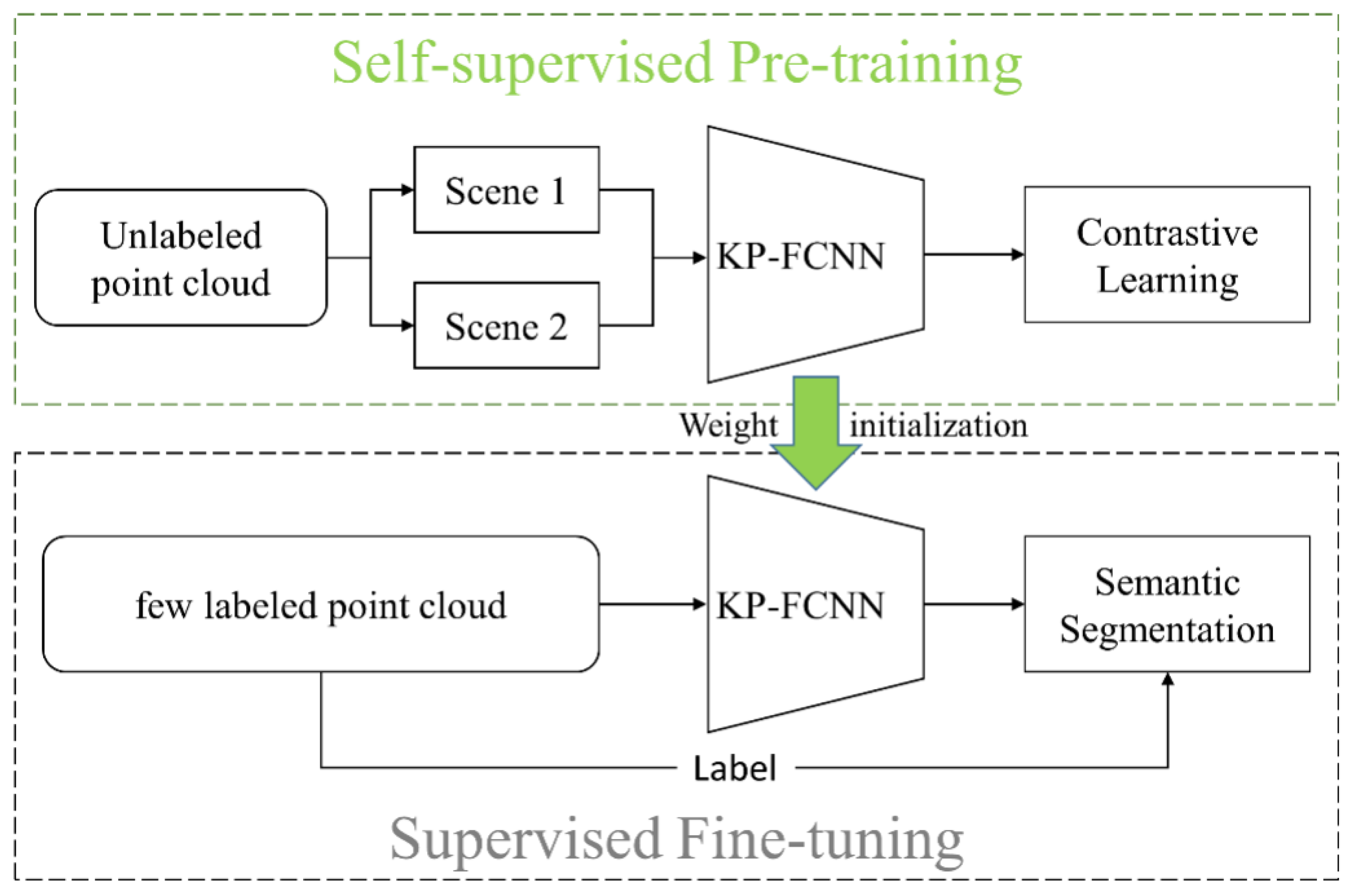
  • A self-supervised contrastive learning scheme is introduced for point cloud semantic segmentation. The meaningful information representation of unlabeled large-scale ALS point clouds is learned using contrastive learning, and then transferred to small local samples for high-level semantic segmentation tasks, resulting in improved semantic segmentation performance.
  • We design AbsPAN, a strategy for selecting positive and negative samples for contrastive learning. This strategy employs an unsupervised clustering algorithm to remove potentially false-negative samples, ensuring that contrastive learning obtains meaningful information.
  • When full of training data are used, the proposed method performed better than the strategy of training from scratch. This means that self-supervised learning is a promising way to improve the performance of deep learning methods for point cloud semantic segmentation.
The remainder of the paper is organized as follows: Section 2 describes the proposed method, and Section 3 illustrates the experiments and analyzes the corresponding results. And, finally, Section 4 concludes this work and gives some outlooks.

2. Methodology

2.1. Overview

The proposed self-supervised learning paradigm for point clouds is illustrated in Figure 1. Our technique aims to utilize unlabeled ALS point clouds to learn spatial invariance by designing self-supervised signals and transferring them to semantic segmentation tasks to reduce the reliance on semantic labels. The proposed method consists of two parts. In the self-supervised pre-training part, contrastive learning is performed on a large-scaled unlabeled point cloud by employing a kernel point fully convolutional network (KP-FCNN) as the backbone. In Figure 1, Scene 1 and Scene 2 refer to two augmented mini-batches of training data. Note that in each epoch of pre-training, we utilize two different augmentation approaches to a same subset of unlabeled point clouds. In the supervised fine-tuning part, the pre-trained weight initiates the downstream semantic segmentation network training and fine-tuning weight on a few labeled point clouds.

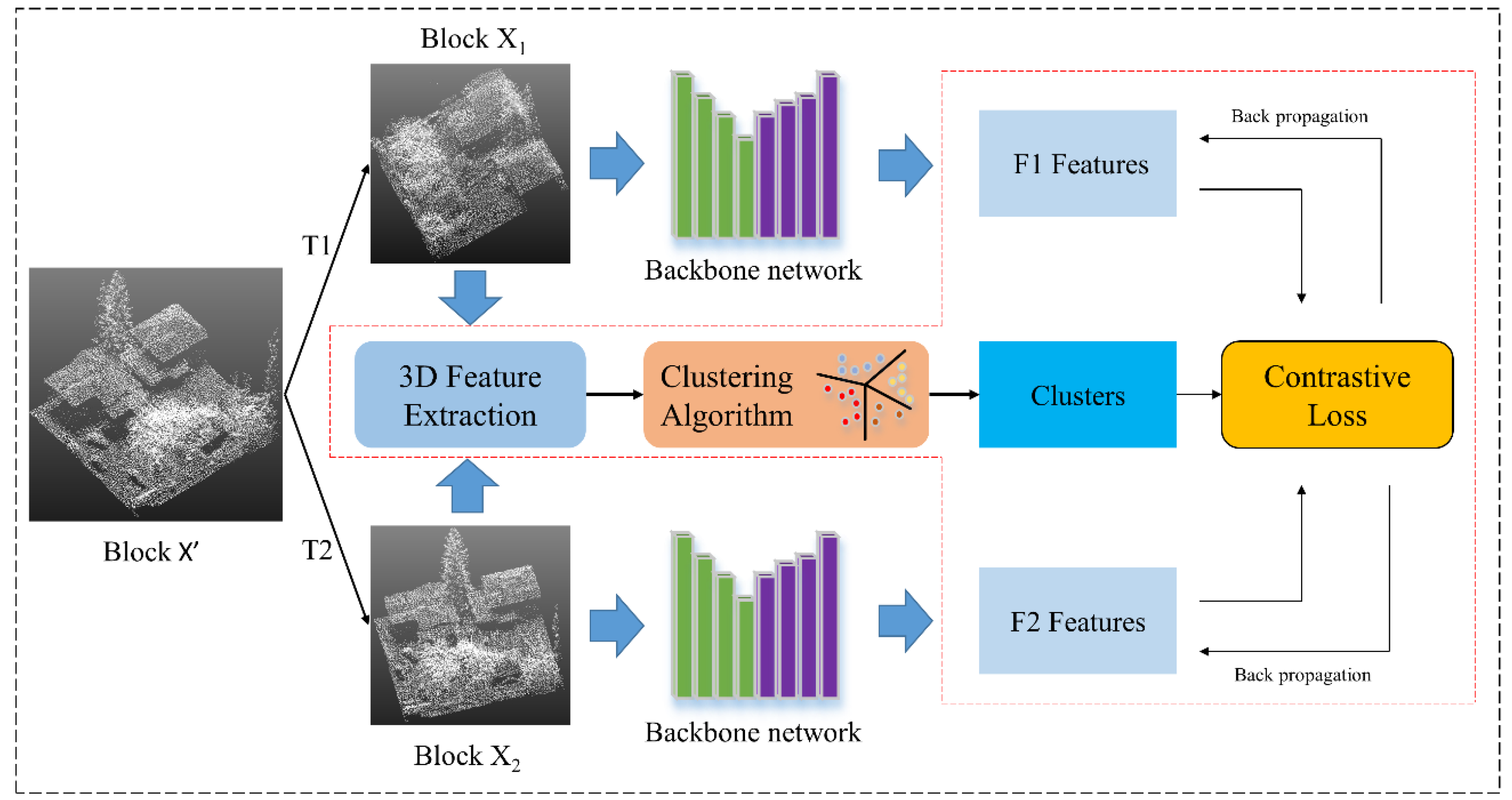
2.2. Point Cloud Contrastive Learning

Self-supervised learning can be implemented by utilizing a variety of specially designed supervised signals, with contrastive learning being selected due to its high representation learning ability. Contrastive learning is an unsupervised approach whose goal is to learn a mapping relationship from the original feature to the embedding space so that the distance function is used to pull positive samples closer together and negative samples apart [31]. Our distance metric function focuses on triplets with hard-negative mining [32]. In particular, as shown in Equation (1), for any anchors x, the objective of the contrastive learning is to obtain an embedding function that meets the following criteria:
L f ( x ) , f x + > > L f ( x ) , f x
where x + are positive samples, and denote points similar or congruent to anchors x. x are negative samples, and denote points dissimilar to anchors x. L is the distance metric function used to measure the similarity between features.
The developed contrastive learning framework is illustrated in Figure 2. The auxiliary pre-training task is described in Section 2.2.1. For the point cloud feature embedding, KP-FCNN is selected as the backbone network and described in Section 2.2.2. The key point of contrastive learning is to construct positive and negative samples. To ensure the purity of these samples, a negative samples mining method based on k-means clustering named “Absolute Positive And Negative samples” (AbsPAN) is proposed and described in detail in Section 2.2.3. Our method optimizes a contrastive loss L c on the extracted high-level features V for a set of a random geometrically transformed point cloud; it is completed by using KP-FCNN. The designed contrastive loss L c is described in Section 2.2.4.

2.2.1. Auxiliary Pre-Task

Inspired by [28], the auxiliary tasks achieve point equivariance concerning a set of random similarity transformations (composed of rotation transformation and scaling; all the similarity transformations hereafter are referred to as rotation transformation and scaling). Concretely, similar to other metric learning algorithms [33,34,35], we define a pair of matching points as a positive pair if they refer to the same point, otherwise they form a negative pair. As illustrated in Figure 2, given a point cloud dataset X = { x 1 , , x i , , x N } , where N is number of all points, a spherical subset X is selected from X by using the random picking strategy using in KP-FCNN, and then two random similarity transformations T1 and T2 are applied to X to obtain pair block X 1 = { x 1 1 , , x 1 i , , x 1 n } , X 2 = { x 2 1 , , x 2 i , , x 2 n } . For each point in block x 1 i , there is a corresponding point x 2 j in block X 2 , ( x 1 i , x 2 j ) are matching points across two blocks. The unsupervised contrastive learning aims at extracting embedding features v s = f ( X s ) , s = { 1 , 2 } , where the embedding function f maps the block to the feature space through the KP-FCNN framework, and X 1 is mapped to V 1 = { v 1 1 , , v 1 i , , v 1 n } , X 2 is mapped to V 2 = { v 2 1 , , v 2 i , , v 2 n } . The matched (positive) point features ( v 1 i , v 2 j ) must be similar to each other and different from unmatched (negative) point features v 2 k . Contrastive learning accomplishes this goal by minimizing the contrastive loss function L c (see Section 2.2.4).

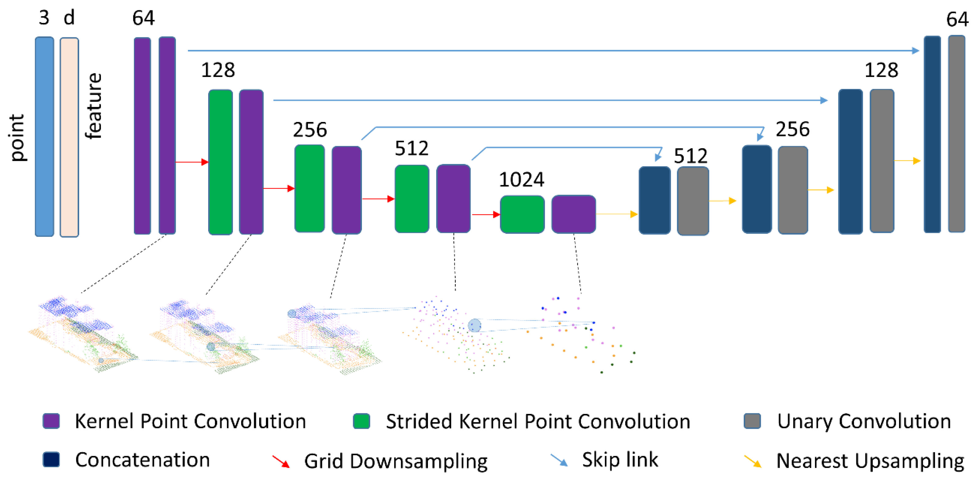
2.2.2. Backbone Network

Since a large amount of data are utilized for pre-training in the proposed contrastive learning strategy, we adopt the KP-FCNN [36] as the backbone network. Because the KP-FCNN stores the data to be processed locally at each layer, this pre-processing step is performed prior to training. Such a strategy increases the training speed. Considering the feature learning ability, the KP-FCNN utilizes strong deformable kernel convolution, which leads to improved object geometry awareness and information aggregation of adjacent categories without confusing them.
The architecture of KP-FCNN is illustrated in Figure 3. The network operates directly on point clouds with position and features. This network uses a kernel point convolution to compute features. In practice, the input of KP-FCNN is a scene block X s . In the five-layer encoder, regular grid sampling is utilized as the downsampling method. In the four-layer decoder, the upsampling method utilizes the nearest sampling. At the end of the forward pass, a feature vector V s , each having 64 dimensions, is obtained.
It is worth noting that self-supervised learning network weights are used for initializing semantic segmentation weights. Slightly different from the pre-training backbone network, a layer of unary convolution is added to the last layer and then realizes the conversion of 64 dimensions to the D o u t dimension in the downstream semantic segmentation task; D o u t is the number of categories. We chose KP-FCNN as a feature extractor, which can be replaced by other deep learning frameworks.

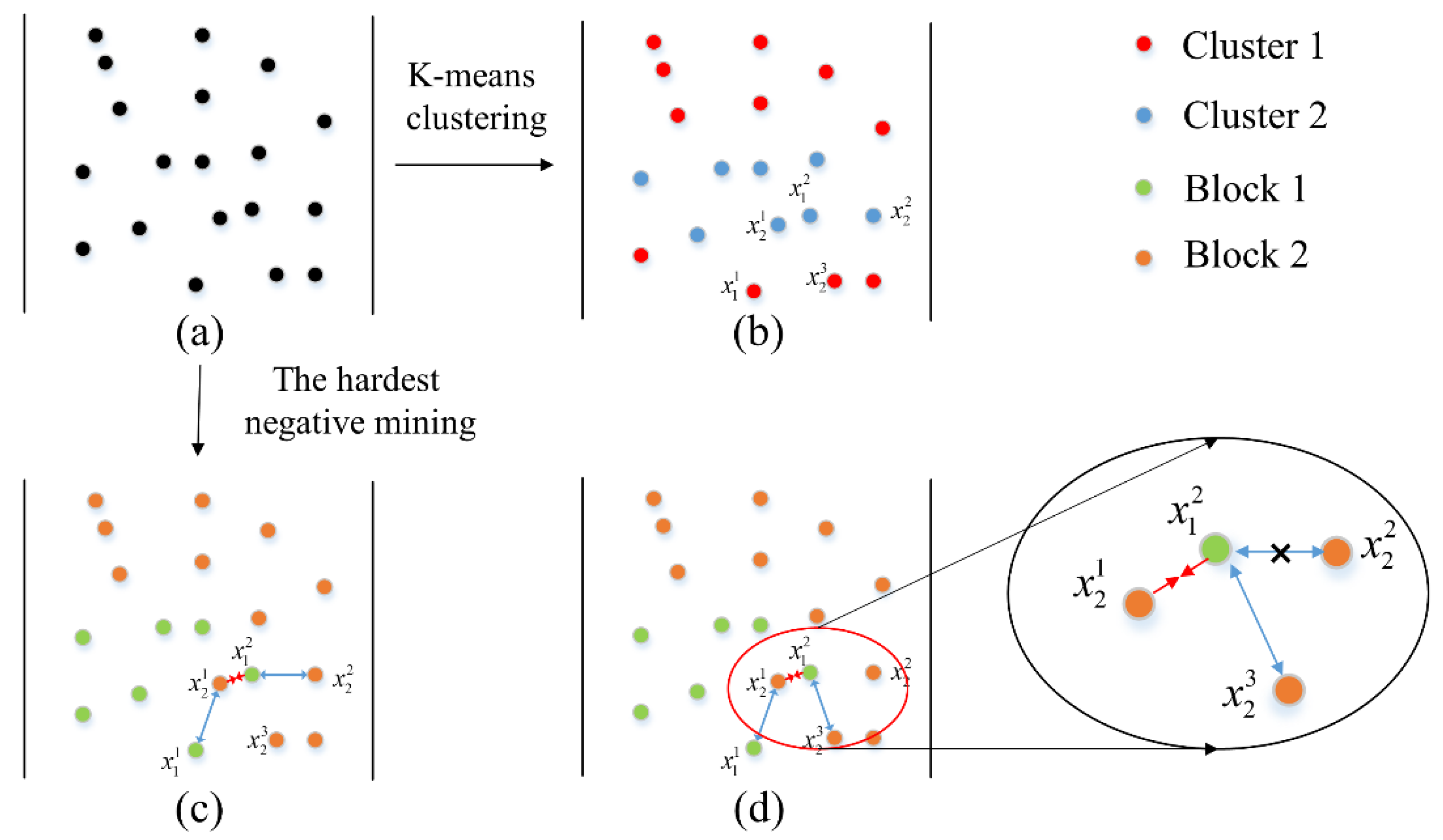
2.2.3. AbsPAN: Negative Samples Mining Based on Clustering

The PointContrast uses the hardest-negative mining scheme (referred to as the hardest-negative mining method hereafter) for subsequent point cloud semantic segmentation [28]. However, changing the number of negatives has no discernible effect on segmentation results [28,37]. This phenomenon contradicts our expectations. This could be because that the hardest negative pairs belong to the same semantic category. To address the issue, we propose a negative samples mining scheme named Absolute Positive and Negative Samples (AbsPAN). The AbsPAN is defined as “a set of representative embeddings of semantically similar instances”, with a focus on identifying “distinguishing negatives”.
Figure 4 illustrated the proposed schematic diagram of the negative samples mining processing. To alleviate the problem that the hardest negative pairs may belong to the same category, the transformed block 1 and 2 are clustered via an unsupervised clustering scheme based on k-means clustering. The clustering processing is performed on traditional handcrafted features, which are listed in Table 1. Because other information, such as intensity, is often unreliable, these features are calculated solely using x-y-z coordinates. For each sample   i , the used geometric are calculated based on covariance tensor i , as shown in Equation (2).
Σ i = 1 N n C i N c n c ¯ c n c ¯
where C i N is the N nearest point set to C i , c ¯ is the medoid in C i N . In Table 1, the eigenvalues λ 1 λ 2 λ 3 0 and corresponding eigenvectors e 1 , e 2 , e 3 can be composed to describe geometric properties. Four handcrafted features, such as surface variation, verticality, normal vector N z and planarity, were selected for the clustering by referring to the relevance metric in previous work [4]. These features are compact and robust, and are profitable for k-means clustering. The details can be found in [4].
Based on clustering, a pseudo label is assigned to each point as shown in Figure 4b. After that, sample pairs are selected as follows:
  • N 1 ( N 1 is experimentally set to 4096 in this paper) anchor point x 1 i is randomly selected in block 1. Then, correspondence matched point x 2 j is chosen as the positive sample for each anchor point x 1 i ;
  • N 2 ( N 2 is experimentally set to 2048 in this paper) anchor points are randomly selected from the pair ( x 1 i , x 2 j ) for the hardest negative sample selection. To ensure that the negative sample belongs to a different category, the point with the closest features (the feature is embedded by the KP-FCNN) to point x 1 i in block 2 is chosen as the hardest negative sample candidate and denoted as x 2 k . If the pseudo label of x 2 k is not equal to x 2 j , x 2 k is a true candidate for the hardest negative sample of x 1 i . Otherwise, x 2 k will be removed and the next point with the nearest feature will be validated until the true candidate is obtained. After getting the hardest negative sample of x 1 i in block 2, the same process will be performed for the x 2 j to search for the hardest negative sample x 1 k in block 1.
Take Figure 4c,d as an example; if only the embedded feature distance is used as in the hardest negative mining algorithm, points x 1 2 and x 2 2 in Figure 4c are regarded as the hardest negative pair. However, these points belonging to the same category would confuse contrastive learning. Based on the pseudo label, points x 1 2 and x 2 3 will be selected as the true hardest negative pair (see Figure 4d) because they are not in the same cluster (see Figure 4b with different colors).

2.2.4. Loss Function Design

After obtaining the negative samples, it is necessary to develop a proper loss function to mine the contrastive semantic information of four types of points ( x 1 i , x 2 j , x 1 , x 2 ) . Inspired by the Hardest-Contrastive loss function [35], the loss function for the auxiliary task is defined as:
L c = ( i , j ) θ d v 1 i , v 2 j t p + 2 | θ | + 0.5 t n Q v 1 i , v 2 k , c i , k + 2 θ i + 0.5 t n Q v 1 k , v 2 j , c k , j + 2 θ j
where the first part of Equation (3) is used to pull closer positive pairs in the learned feature space, and the latter two parts of Equation (3) are used to push apart negative samples. θ is a set of matched (positive) pairs, the hardest negative sample is defined as the point closest to the positive pair in the L 2 standardized feature space, L 2 = m v 1 v 2 2 , m is the output feature dimension by KP-FCNN. v 1 i and v 2 j are output features of the matched pair, v k is the hardest negative sample. d ( v 1 i , v 2 j ) is the distance between v 1 i and v 2 j . c i , k = { 1 , i f g ( x 1 i x 2 k ) ; e l s e 0 } , where g ( · ) is the cluster obtained from k-means clustering in handcrafted geometric features space. Q ( v 1 i , v 2 k , c i , k ) is the nearest distance between the feature of a negative pair under the condition that g ( x 1 i x 2 k ) , Q ( v 1 i , v 2 k , c i , k ) for the x 1 k and x 2 j similarly. [ x ] + = m a x ( 0 , x ) , | θ | denotes number of the valid mined negative sample for v 2 j . t p and t n are the margins of positive and negative pairs.

3. Experiments

This section evaluates the proposed self-supervised learning method on several benchmark ALS point clouds. The proposed method is implemented via the PyTorch framework, on an Intel CoreTM i7-11700F CPU utilizing an NVIDIA RTX 3090 GPU with 24 GB memory.

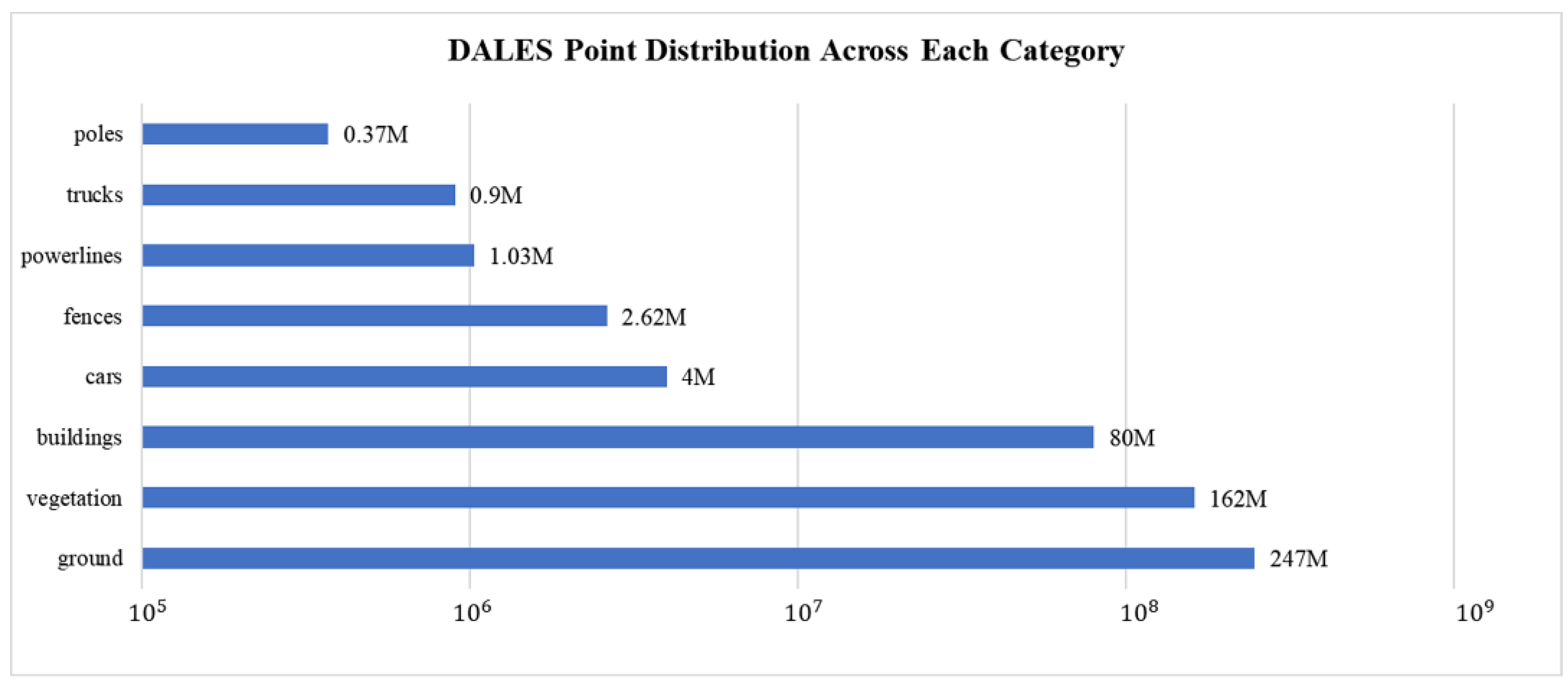
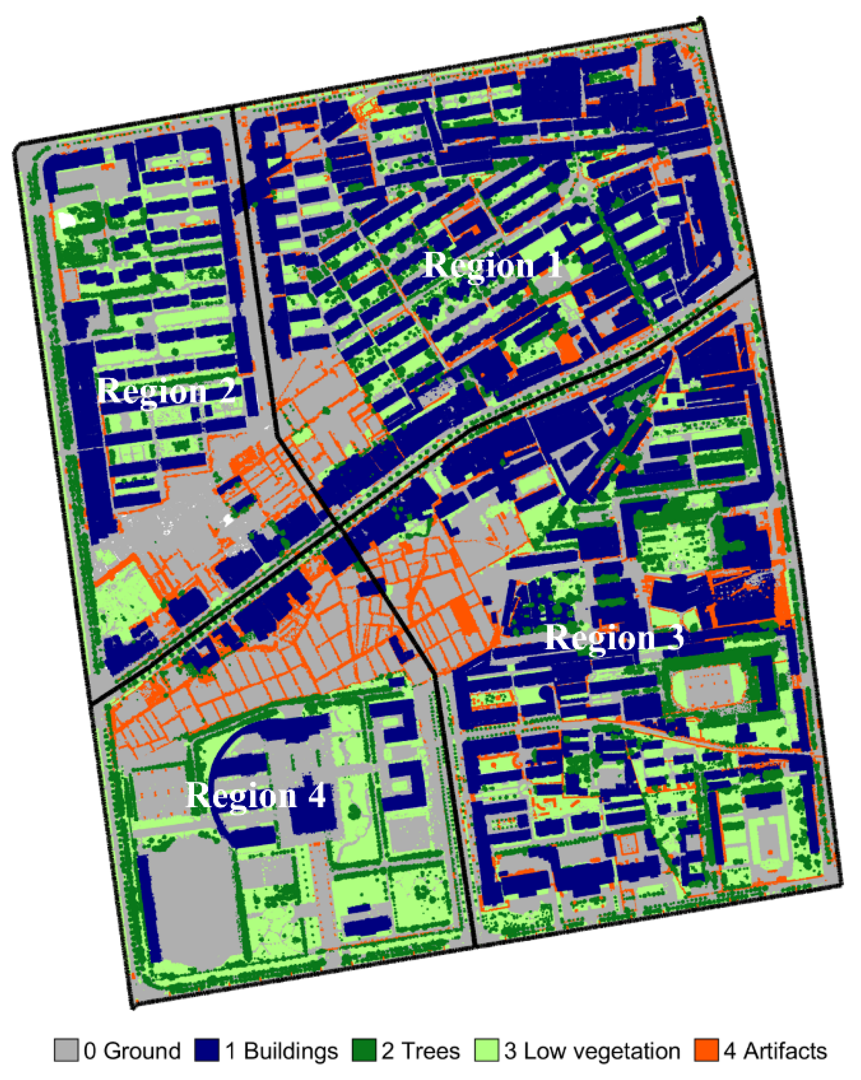
3.1. Experimental Dataset

Data for the auxiliary task. We considered the integrated scene categories and scales in the upstream auxiliary task and chose the DALES [38] point cloud dataset, which is divided into 40 non-overlapping scenes, each of which covers 0.5 and more than 12 million points. The point cloud density is about 50 points. The number of points in each category is presented in Figure 5.
Data for the semantic segmentation task. In the downstream semantic segmentation task, we utilize the Vaihingen 3D semantic labeling benchmark dataset provided by ISPRS [6]. Each point contains spatial coordinates (XYZ), intensity values, and the number of returns. The five attributes mentioned above are used as the network’s input. According to the official division, the Vaihingen dataset has two parts: the training and the testing set.
In order to verify the effectiveness of the self-supervised model under the scenario of insufficient labeled data, and considering the distribution and quantity of each category, we exploit 10%, 20%, 40%, 60% and 100% of the training data to fine-tune the downstream semantic segmentation. The point cloud area is depicted in Figure 6 and Figure 7.
In addition to the ISPRS Vaihingen 3D data sets, we also utilize the LASDU dataset for verification, which was collected in the Heihe River Basin, Northwestern China. This dataset is divided into four regions, and the total number of points for all regions is 3.12 million. Each point contains its spatial coordinates (XYZ) and intensity value. Regions 2 and 3, illustrated in Figure 8, are used as the training set, while Regions 1 and 4 are used as the test set.

3.2. Evaluation Metrics

We evaluate our method’s segmentation performance utilizing the overall accuracy (OA) and average F1 score (Avg. F1). OA is the percentage of the correctly classified point out to the total points, and the F1 score is the harmonic average of the precision and recall of each category, defined as:
OA = ( T P + T N ) / t o t a l Precision = T P / ( T P + F P ) Recall = T P / ( T P + F N ) F 1 Score = 2 × Precision × Recall Precision + Recall
where total, TP, FP, and FN are all samples, the true positive, false positive, and false negative, respectively.

3.3. Parameters Set Up

Parameters and preprocessing for the pre-training contrastive learning task. During data processing, we employed 0.4 m as the grid sampling value to deal with extreme point cloud density variations. Moreover, from the entire point cloud, we randomly extract the vertices within a spherical volume, which are input to the network. We use the constant feature equal to 1, normalized intensity, and normalized Z-coordinates within the sphere as input features. The sphere’s radius is set to 10 m, large enough to include several objects. The amount of kernel points in the convolution operator is 19, properly set to balance computational cost and descriptive power. All five-layer networks involve a downsampling process, while the convolution radius of each layer and the downsampling grid size are presented in Table 2. During importing the two blocks for the contrastive learning process, the input point cloud is randomly rotated (0°∼360°) and scaled (0.8∼1.2) to augment it. For the hardest negative sample mining, we do not have to use all the points for mining, only a portion of the points are considered in the loss function [27,39,40]. The parameter K for the k-means clustering algorithm is set to 9. For the contrastive learning loss, the number of positive pairs is set to 4096, and the number of negative samples is set to 2048. Details about the quantity of positive and negative samples can be found in [35]. The threshold distance of the negative samples is set to 2.0, and for the positive samples is set to 0.2.
The stochastic gradient descent (SGD) optimization algorithm is employed as the optimizer, with the learning rate starting from 0.001. One epoch involves 8000 iterations, and the model is trained for 50,000 epochs.
Parameters and preprocessing for the downstream semantic segmentation task. During dataset selection, datasets with insufficient data are selected on priority, thus the ISPRS and LASDU datasets are utilized to verify the gain afforded by self-supervision. During training data processing, we use grid sampling of 0.4 m, which is similar to the hyper-parameter setting process for the auxiliary tasks. For ISPRS datasets, we use the constant 1, intensity values, the number of returns and normalized Z-coordinates within the sphere as input 4D vector features. For LASDU datasets, we add intensity values and normalized Z-coordinates as additional features to the constant 1, as input 3D vector. In the training stage, spheres are randomly selected into the network. In the testing stage, spheres are regularly selected, and each point is tested more than 20 times. Obviously, we aim to test all the points in test set to ensure the integrity. In addition, such an approach is similar to a voting scheme, we are able to obtain the average predicted value to evaluate the testing stage. As a result, the sphere’s boundary points are well protected.
For the network parameters, the sphere’s radius is set to 10 m, and the number of kernel points is set to 19. The convolution radius and the down-sampling grid size for each layer are presented in Table 2. The learning rate is set to 0.001, the batch size to 4, and the decay rate is set to 0.98 at every five epochs. We train the model for 200 iterations in one epoch, and the convergence is expected after 50 epochs.

3.4. Experimental Results and Analysis

3.4.1. Effectiveness of SSL

We prove the efficiency of our self-supervised learning network on data comprehension. Therefore, we artificially tailor the ISPRS training scene randomly so that the amount of training data are only about 10% of the original training data. This strategy emphasizes the information gain provided by our self-supervised framework for downstream semantic segmentation tasks.
The segmentation results on the test data of the Vaihingen 3D dataset are reported in Table 3. We also compare our method with other published models, such as PointNet++ [15], PointSIFT [16], KP-FCNN [36], D-FCN [41], RandLA-Net [26], and DPE [42]. We regard the results of these methods as a reference and use KP-FCNN as the baseline model. The baseline networks are trained from scratch, while Table 3 presents the fine-tuned results of our HAVANA method using the pre-trained weights. It can be seen that our HAVANA trained with 100% training data achieves competitive improvement with fully supervised models on the Vaihingen 3D test data. When reducing the training points to only 10%, the proposed method outperforms the baseline approaches based on KP-FCNN, especially for small-numbered categories like cars and fences. When only 10% labeled training data are used for fine-tuning, our HAVANA method outperforms the baseline model, increasing OA up to 3.9% and Avg.F1 by 3.2%. The benefits of introducing unlabeled data to self-supervised learning are obvious. This proves that the proposed self-supervised methods effectively exploit the information learned from the auxiliary pre-tasks. It is worth mentioning that improving the fully supervised model with limited training data is worthwhile.
Figure 9 illustrates visualized classification results and the error map using our HAVANA method on the 100% Vaihingen 3D training dataset. The classification results show that HAVANA performs well in classification on the test set. From the error map, we can see that the labels of the majority of points can be predicted correctly. With reference to the visualized classification results, the majority of roof and impervious surfaces could be correctly classified. For the misclassified points, it is easy to find that facades are easily divided into roofs and fences into low vegetation. These categories indeed have similar geometric properties, local features are similar in neighborhood aggregation, and self-supervision improvement is also limited.

3.4.2. Hardest-Contrastive vs. AbsPAN

In the subsequent trials, we compare the proposed HAVANA method against the Hardest-Contrastive strategy, a positive and negative sample selection strategy proposed in [28], with the corresponding results presented in Table 4. The originally reported Hardest-Contrastive strategy [28] utilizes the MinkowskiNet as the backbone network. Therefore, for a fair comparison, we replace the KP-FCNN with MinkowskiNet in our network, and present a KP-FCNN variant with the Hardest-Contrastive strategy.
For comparison, we only use 10% of the Vaihingen 3D training data for fine-tuning. By comparing MinkowskiNet and KP-FCNN, we find that KP-FCNN performs better on the proposed pipeline. The corresponding results reveal that if MinkowskiNet is used, the proposed AbsPAN presents improves OA and Avg.F1 by 0.4% and 1.9%, respectively, against the Hardest-Contrastive method. Under the KP-FCNN learning framework, the improvement is 0.9% and 1.0% for OA and Avg. F1, respectively.

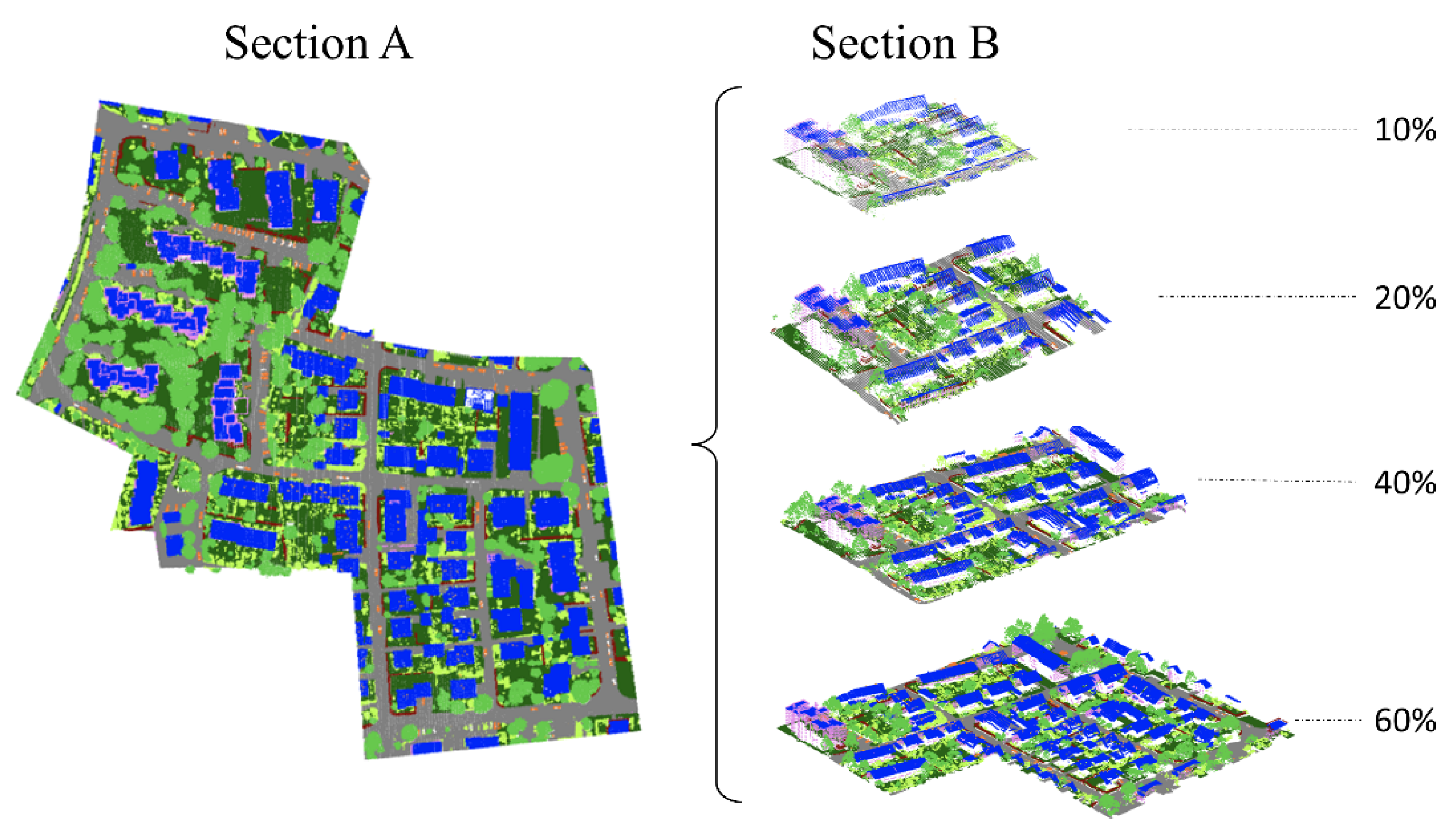
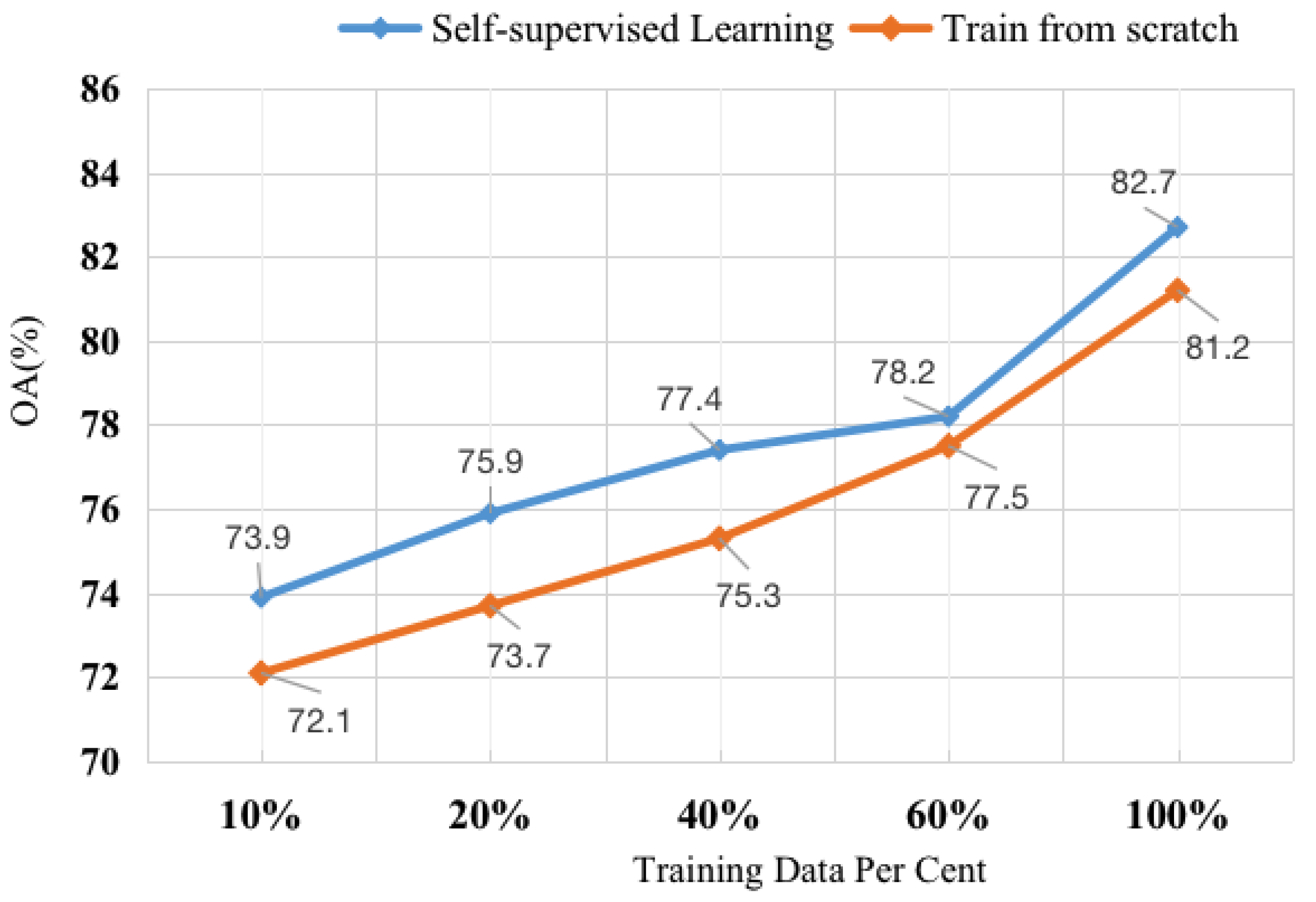
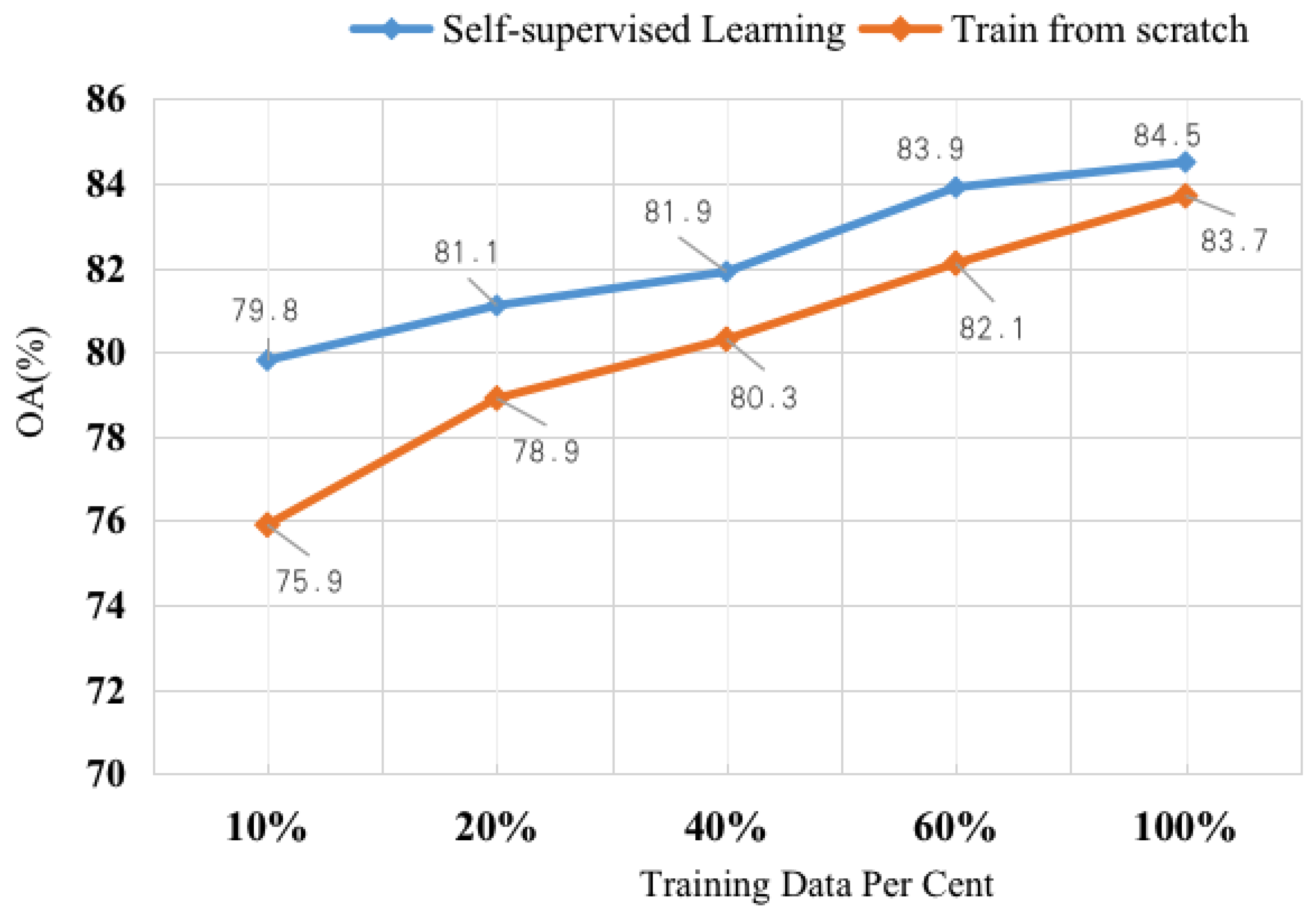
3.4.3. Performance with Different Amounts of Training Data

In order to explore the ability of self-supervised learning to understand ALS point cloud scenes efficiently, we set up our contrastive learning framework (frame selection is biased towards lightweight model) to illustrate the adaptive changes in self-supervised learning under the five subsets of training data. Due to the uneven class distribution in the Vaihingen 3D dataset, as the area is too small to include all categories, we crop five subsets {10%, 20%, 40%, 60%, 100%} of the training area belonging to the official training set by ISPRS. The results are presented in Figure 10 and Figure 11. “Self-supervised Learning” denotes the result of fine-tuning with our pre-trained weights, and “Train from scratch” denotes the result of the train from scratch baseline.
For the experimental results, we take the average of the three experimental groups to reduce the impact of the variance. For the two baseline frameworks, we use the same experimental settings, and observe OA difference between fine-tuned with our pre-trained weights and trained from scratch under different training subsets, self-supervised pre-training weights are used for initialization methods have significantly improved the accuracy of semantic segmentation compared to training from scratch. From Figure 10 and Figure 11, the trend is clear: the fewer semantic labels used for training, the greater the improvement in SSL. When the 10% labeled data are imported into the network, the OA improvement of the PointNet++ and KP-FCNN due to SSL is 1.8% and 3.9%, respectively. As the amount of semantic label data increases, the gap between self-supervision learning and direct training from scratch becomes smaller. It can be concluded that when labeled training data are insufficient, the proposed self-supervision learning is very important. However, the results show that using the SSL method under 10% of the training data still gives worse results than training from scratch using 100% of the training data. Thus, if possible, labeling more samples is a good way to ensure classification accuracy.

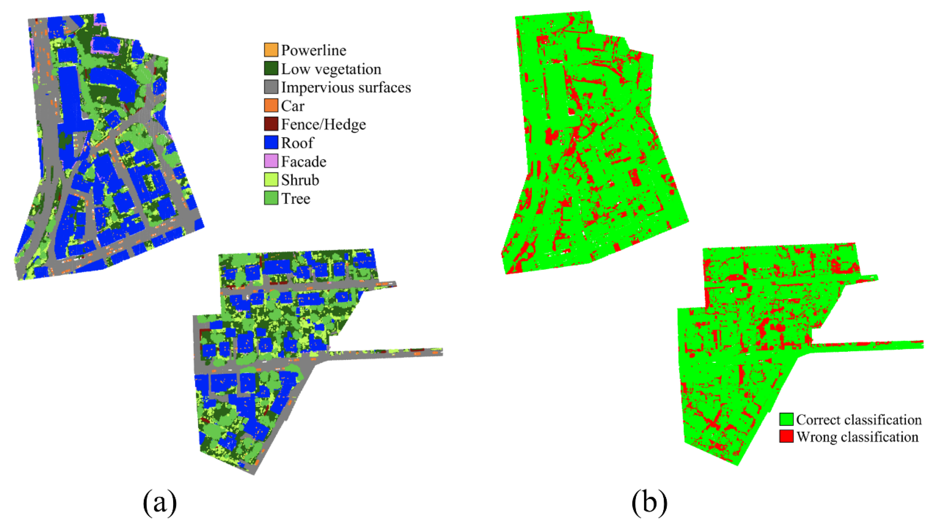
3.4.4. Further Experiment Results

To verify that the proposed HAVANA model is also improved on other ALS point clouds, the LASDU dataset [43] specifically designed for the semantic segmentation of ALS point clouds in dense urban areas is chosen for further experiments. The proposed HAVANA method with KP-FCNN as the backbone is pre-trained on the DALES dataset, and then it is fine-tuned on the training data of the LASDU dataset. After that, the model is tested on the test set of the LASDU dataset. The results are shown in Table 5, where the results of the baseline methods are the ones reported in the related references, including PointNet++ [15], PointSIFT [16], KP-FCNN [36], DPE [42], and GraNet [44]. These methods are all full-supervised methods and training from scratch with LASDU official training.
It can be found from the results that the proposed self-supervised method performed best on the LASDU dataset, and all five categories achieved the best performance. For the artifacts category with few training samples, the F1 score is improved by 3%, which benefits from the representation learning in the self-supervised auxiliary task. The OA of the HAVANA method reached 87.6%, and the Avg. F1 reached 77.5%, achieving state-of-the-art performance.
Figure 12 visualizes the classification results of our HAVANA method on the LASDU dataset, highly realistic to the real urban scenery dataset. On LASDU dataset, our method achieves an appealing performance, highlighting the significance of our method. Looking at the classification error map of the LASDU dataset in Figure 13, Most of the regions can be classified correctly, with a few partially incorrectly classified regions. With regard to Figure 9, it is easy to find that the building’s boundary classification is clearer, presenting obvious linear boundaries. This is a question worthy of further study.
To sum up, compared with reported baseline methods, two aspects of conclusions can be summarized: (1) The proposed methods is competitive with 100% labeled training data, outperforms supervised baseline methods with limited labeled training data. (2) Self-supervised contrastive learning pre-training with large amounts of unlabeled point clouds is helpful for initializing network parameters, which can be further fine-tuned by limited label data for downstream tasks, like semantic segmentation.

4. Conclusions

This paper proposes a contrastive learning strategy for point clouds, a general unsupervised representation learning framework that performs iterative clustering and guides the feature learning direction. Through the ALS point cloud, the experiment shows SSL has great potential for point cloud semantic segmentation tasks when the label is limited. The point cloud knowledge learned by our auxiliary task can be transferred to the downstream semantic classification task. Furthermore, the proposed method is easily integrated with a variety of deep learning frameworks. In the case of aerial laser point clouds with insufficient semantic labels, our experiments demonstrate the superiority of self-supervised contrastive learning. We conclude that self-supervision learning is clearly advantageous for semantic segmentation of limited labeled ALS point clouds.
There are also some limitations in the proposed method KP-FCNN is a baseline network using geometric convolution to encode local point-wise features, which shall be improved to structure learning. The proposed method is convinced that better selecting negative samples are beneficial for contrastive learning, and it is worth investigating more robust sampling strategies for positive and negative samples in the future.

Author Contributions

Conceptualization, Y.Z.; methodology, J.Y. and Y.Z.; software, J.Y., R.Z. and S.C.; validation, J.Y. and H.F.; data curation, J.Y.; writing—original draft preparation, Y.Z., R.Z. and J.Y.; writing—review and editing, X.W. and H.F. All authors have read and agreed to the published version of the manuscript.

Funding

This work was partially supported by National Natural Science Foundation of China, under Grant 42171440; Science and Technology Research and Development Program Project of China railway group limited (Major Special Project), under the Grant 2021-Special-08; Major S&T Program of Hunan Province, under the Grant 2020GK1023; The research Project of PowerChina Zhongnan Engineering Corporation Limited, under the Grant YF-A-2020-05-1.

Conflicts of Interest

Author Yunsheng Zhang was employed by the company PowerChina Zhongnan Engineering Corporation Limited and Author Han Fu was employed by the company Space Star Technology Co., Ltd. The remaining authors declare that the research was conducted in the absence of any commercial or financial relationships that could be construed as a potential conflict of interest.

References

  1. Liu, X. High technologies of surveying and mapping for social progress. Sci. Surv. Mapp. 2019, 44, 1–15. [Google Scholar]
  2. Guo, R.; Lin, H.; He, B.; Zhao, Z. GIS framework for smart cities. Geomat. Inf. Sci. Wuhan Univ. 2020, 45, 1829–1835. [Google Scholar]
  3. Liu, W.; Zang, Y.; Xiong, Z.; Bian, X.; Wen, C.; Lu, X.; Wang, C.; Junior, J.M.; Gonçalves, W.N.; Li, J. 3D building model generation from MLS point cloud and 3D mesh using multi-source data fusion. Int. J. Appl. Earth Obs. Geoinf. 2023, 116, 103171. [Google Scholar] [CrossRef]
  4. Weinmann, M.; Schmidt, A.; Mallet, C.; Hinz, S.; Rottensteiner, F.; Jutzi, B. Contextual classification of point cloud data by exploiting individual 3D neigbourhoods. ISPRS Ann. Photogramm. Remote Sens. Spat. Inf. Sci. II-3 2015, 2, 271–278. [Google Scholar] [CrossRef]
  5. Weinmann, M.; Jutzi, B.; Hinz, S.; Mallet, C. Semantic point cloud interpretation based on optimal neighborhoods, relevant features and efficient classifiers. ISPRS J. Photogramm. Remote Sens. 2015, 105, 286–304. [Google Scholar] [CrossRef]
  6. Niemeyer, J.; Rottensteiner, F.; Soergel, U. Contextual classification of lidar data and building object detection in urban areas. ISPRS J. Photogramm. Remote Sens. 2014, 87, 152–165. [Google Scholar] [CrossRef]
  7. Rusu, R.B.; Marton, Z.C.; Blodow, N.; Dolha, M.; Beetz, M. Towards 3D point cloud based object maps for household environments. Robot. Auton. Syst. 2008, 56, 927–941. [Google Scholar] [CrossRef]
  8. Tombari, F.; Salti, S.; Di Stefano, L. Unique signatures of histograms for local surface description. In Proceedings of the Computer Vision–ECCV 2010: 11th European Conference on Computer Vision, Heraklion, Greece, 5–11 September 2010; pp. 356–369. [Google Scholar]
  9. Jie, S.; Zulong, L. Airborne LiDAR Feature Selection for Urban Classification Using Random Forests. Geomat. Inf. Sci. Wuhan Univ. 2014, 39, 1310. [Google Scholar]
  10. Weinmann, M. Feature relevance assessment for the semantic interpretation of 3D point cloud data. ISPRS Ann. Photogramm. Remote Sens. Spat. Inf. Sci. 2013, 2, 313–318. [Google Scholar] [CrossRef]
  11. Zhao, R.; Pang, M.; Wang, J. Classifying airborne LiDAR point clouds via deep features learned by a multi-scale convolutional neural network. Int. J. Geogr. Inf. Sci. 2018, 32, 960–979. [Google Scholar] [CrossRef]
  12. Schmohl, S.; Sörgel, U. Submanifold sparse convolutional networks for semantic segmentation of large-scale ALS point clouds. ISPRS Ann. Photogramm. Remote Sens. Spat. Inf. Sci. 2019, 4, 77–84. [Google Scholar] [CrossRef]
  13. Tchapmi, L.; Choy, C.; Armeni, I.; Gwak, J.; Savarese, S. Segcloud: Semantic segmentation of 3d point clouds. In Proceedings of the 2017 international conference on 3D vision (3DV), Qingdao, China, 10–12 October 2017; pp. 537–547. [Google Scholar]
  14. Qi, C.R.; Su, H.; Mo, K.; Guibas, L.J. Pointnet: Deep learning on point sets for 3d classification and segmentation. In Proceedings of the IEEE conference on computer vision and pattern recognition, Honolulu, HI, USA, 21–26 July 2017; pp. 652–660. [Google Scholar]
  15. Qi, C.R.; Yi, L.; Su, H.; Guibas, L.J. Pointnet++: Deep hierarchical feature learning on point sets in a metric space. Adv. Neural Inf. Process. Syst. 2017, 30. [Google Scholar] [CrossRef]
  16. Jiang, M.; Wu, Y.; Zhao, T.; Zhao, Z.; Lu, C. Pointsift: A sift-like network module for 3d point cloud semantic segmentation. arXiv 2018, arXiv:1807.00652. [Google Scholar]
  17. Arief, H.A.; Indahl, U.G.; Strand, G.H.; Tveite, H. Addressing overfitting on point cloud classification using Atrous XCRF. ISPRS J. Photogramm. Remote Sens. 2019, 155, 90–101. [Google Scholar] [CrossRef]
  18. Wen, C.; Li, X.; Yao, X.; Peng, L.; Chi, T. Airborne LiDAR point cloud classification with global-local graph attention convolution neural network. ISPRS J. Photogramm. Remote Sens. 2021, 173, 181–194. [Google Scholar] [CrossRef]
  19. Shorten, C.; Khoshgoftaar, T.M. A survey on image data augmentation for deep learning. J. Big Data 2019, 6, 1–48. [Google Scholar] [CrossRef]
  20. Wang, P.; Yao, W. A new weakly supervised approach for ALS point cloud semantic segmentation. ISPRS J. Photogramm. Remote Sens. 2022, 188, 237–254. [Google Scholar] [CrossRef]
  21. Lei, X.; Guan, H.; Ma, L.; Yu, Y.; Dong, Z.; Gao, K.; Delavar, M.R.; Li, J. WSPointNet: A multi-branch weakly supervised learning network for semantic segmentation of large-scale mobile laser scanning point clouds. Int. J. Appl. Earth Obs. Geoinf. 2022, 115, 103129. [Google Scholar] [CrossRef]
  22. Wang, Y.; Zhang, J.; Kan, M.; Shan, S.; Chen, X. Self-supervised equivariant attention mechanism for weakly supervised semantic segmentation. In Proceedings of the IEEE/CVF Conference on Computer Vision and Pattern Recognition, Seattle, WA, USA, 13–19 June 2020; pp. 12275–12284. [Google Scholar]
  23. Ayush, K.; Uzkent, B.; Meng, C.; Tanmay, K.; Burke, M.; Lobell, D.; Ermon, S. Geography-aware self-supervised learning. In Proceedings of the IEEE/CVF International Conference on Computer Vision, Montreal, BC, Canada, 11–17 October 2021; pp. 10181–10190. [Google Scholar]
  24. Sharma, C.; Kaul, M. Self-supervised few-shot learning on point clouds. Adv. Neural Inf. Process. Syst. 2020, 33, 7212–7221. [Google Scholar]
  25. Liu, Y.; Yi, L.; Zhang, S.; Fan, Q.; Funkhouser, T.; Dong, H. P4Contrast: Contrastive Learning with Pairs of Point-Pixel Pairs for RGB-D Scene Understanding. arXiv 2020, arXiv:1807.00652. [Google Scholar]
  26. Hu, Q.; Yang, B.; Xie, L.; Rosa, S.; Guo, Y.; Wang, Z.; Trigoni, N.; Markham, A. Randla-net: Efficient semantic segmentation of large-scale point clouds. In Proceedings of the IEEE/CVF conference on computer vision and pattern recognition, Seattle, WA, USA, 13–19 June 2020; pp. 11108–11117. [Google Scholar]
  27. Rao, Y.; Lu, J.; Zhou, J. Global-local bidirectional reasoning for unsupervised representation learning of 3d point clouds. In Proceedings of the IEEE/CVF Conference on Computer Vision and Pattern Recognition, Seattle, WA, USA, 13–19 June 2020; pp. 5376–5385. [Google Scholar]
  28. Xie, S.; Gu, J.; Guo, D.; Qi, C.R.; Guibas, L.; Litany, O. Pointcontrast: Unsupervised pre-training for 3d point cloud understanding. In Proceedings of the Computer Vision–ECCV 2020: 16th European Conference, Glasgow, UK, 23–28 August 2020; pp. 574–591. [Google Scholar]
  29. Sauder, J.; Sievers, B. Self-supervised deep learning on point clouds by reconstructing space. Adv. Neural Inf. Process. Syst. 2019, 32, 12962–12972. [Google Scholar]
  30. Poursaeed, O.; Jiang, T.; Qiao, H.; Xu, N.; Kim, V.G. Self-supervised learning of point clouds via orientation estimation. In Proceedings of the 2020 International Conference on 3D Vision (3DV), Fukuoka, Japan, 25–28 November 2020; pp. 1018–1028. [Google Scholar]
  31. Chen, T.; Kornblith, S.; Norouzi, M.; Hinton, G. A simple framework for contrastive learning of visual representations. In Proceedings of the International Conference on Machine Learning, Virtual, 13–18 July 2020; pp. 1597–1607. [Google Scholar]
  32. Wang, J.; Song, Y.; Leung, T.; Rosenberg, C.; Wang, J.; Philbin, J.; Chen, B.; Wu, Y. Learning fine-grained image similarity with deep ranking. In Proceedings of the IEEE Conference on Computer Vision and Pattern Recognition, Columbus, OH, USA, 23–28 June 2014; pp. 1386–1393. [Google Scholar]
  33. Oh Song, H.; Xiang, Y.; Jegelka, S.; Savarese, S. Deep metric learning via lifted structured feature embedding. In Proceedings of the IEEE Conference on Computer Vision and Pattern Recognition, Las Vegas, NV, USA, 27–30 June 2016; pp. 4004–4012. [Google Scholar]
  34. Sohn, K. Improved deep metric learning with multi-class n-pair loss objective. Adv. Neural Inf. Process. Syst. 2016, 29. Available online: https://dl.acm.org/doi/10.5555/3157096.3157304 (accessed on 14 January 2024).
  35. Choy, C.; Park, J.; Koltun, V. Fully convolutional geometric features. In Proceedings of the IEEE/CVF International Conference on Computer Vision, Seoul, Republic of Korea, 27 October–2 November 2019; pp. 8958–8966. [Google Scholar]
  36. Thomas, H.; Qi, C.R.; Deschaud, J.E.; Marcotegui, B.; Goulette, F.; Guibas, L.J. Kpconv: Flexible and deformable convolution for point clouds. In Proceedings of the IEEE/CVF International Conference on Computer Vision, Seoul, Republic of Korea, 27–28 October 2019; pp. 6411–6420. [Google Scholar]
  37. Hou, J.; Graham, B.; Nießner, M.; Xie, S. Exploring data-efficient 3d scene understanding with contrastive scene contexts. In Proceedings of the IEEE/CVF Conference on Computer Vision and Pattern Recognition, Nashville, TN, USA, 20–25 June 2021; pp. 15587–15597. [Google Scholar]
  38. Varney, N.; Asari, V.K.; Graehling, Q. DALES: A large-scale aerial LiDAR data set for semantic segmentation. In Proceedings of the IEEE/CVF Conference on Computer Vision and Pattern Recognition Workshops, Seattle, WA, USA, 14–19 June 2020; pp. 186–187. [Google Scholar]
  39. Choy, C.; Gwak, J.; Savarese, S. 4d spatio-temporal convnets: Minkowski convolutional neural networks. In Proceedings of the IEEE/CVF Conference on Computer Vision and Pattern Recognition, Long Beach, CA, USA, 15–20 June 2019; pp. 3075–3084. [Google Scholar]
  40. Zhang, Z.; Girdhar, R.; Joulin, A.; Misra, I. Self-supervised pretraining of 3d features on any point-cloud. In Proceedings of the IEEE/CVF International Conference on Computer Vision, Virtual, 11–17 October 2021; pp. 10252–10263. [Google Scholar]
  41. Wen, C.; Yang, L.; Li, X.; Peng, L.; Chi, T. Directionally constrained fully convolutional neural network for airborne LiDAR point cloud classification. ISPRS J. Photogramm. Remote Sens. 2020, 162, 50–62. [Google Scholar] [CrossRef]
  42. Huang, R.; Xu, Y.; Hong, D.; Yao, W.; Ghamisi, P.; Stilla, U. Deep point embedding for urban classification using ALS point clouds: A new perspective from local to global. ISPRS J. Photogramm. Remote Sens. 2020, 163, 62–81. [Google Scholar] [CrossRef]
  43. Ye, Z.; Xu, Y.; Huang, R.; Tong, X.; Li, X.; Liu, X.; Luan, K.; Hoegner, L.; Stilla, U. Lasdu: A large-scale aerial lidar dataset for semantic labeling in dense urban areas. ISPRS Int. J. Geo-Inf. 2020, 9, 450. [Google Scholar] [CrossRef]
  44. Huang, R.; Xu, Y.; Stilla, U. GraNet: Global relation-aware attentional network for semantic segmentation of ALS point clouds. ISPRS J. Photogramm. Remote Sens. 2021, 177, 1–20. [Google Scholar] [CrossRef]
Figure 1. The self-supervised learning paradigm for point cloud semantic segmentation.
Remotesensing 16 00485 g001
Figure 2. Illustration of contrastive learning. For the backbone network, the green bars are encoders and the purple bars are decoders. The circled part of the red line represents our “AbsPAN” strategy selecting both positive and negative samples and optimizing the loss function.
Remotesensing 16 00485 g002
Figure 3. Illustration of the backbone network. The encoder (the first five layers) contains two convolutional blocks, kernel point convolution (KPConv) and strided kernel point convolution. The decoder (the last four layers) uses the nearest upsampling, ensuring that the pointwise feature is added up. The features transferred from the encoder layer are concatenated to the upsampled ones by skip links. The concatenated features are processed by the unary convolution, which is the equivalent of shared multi-layer perceptron (MLP) in PointNet.
Remotesensing 16 00485 g003
Figure 4. Illustration of negative samples mining processing: (a) raw point clouds; (b) clustering results, (c) hardest negative candidates, (d) AbsPAN results. Among them, the orange points represent block 1, and the green points represent block 2; (c) is in the embedding feature space of the network; (b) is the clustering result by k-means in geometric feature space, the red points represent cluster 1, and the blue points represent cluster 2.
Remotesensing 16 00485 g004
Figure 5. DALES point distribution across object categories.
Remotesensing 16 00485 g005
Figure 6. ISPRS training set. Section A (left) is the full training set. Section B (right) shows the subsets of training data cropped from all training sets. The five subsets have the same category distribution.
Remotesensing 16 00485 g006
Figure 7. ISPRS Vaihingen test set.
Remotesensing 16 00485 g007
Figure 8. LASDU data set. Annotated dataset with points of different labels presented in different colors. The black border divides the entire area into four separate regions.
Remotesensing 16 00485 g008
Figure 9. Classification results. (a) Visualized classification results of our HAVANA on the ISPRS test set, (b) error map of our HAVANA on the Vaihingen 3D dataset.
Remotesensing 16 00485 g009
Figure 10. Overall accuracy of different subsets in PointNet++ framework.
Remotesensing 16 00485 g010
Figure 11. Overall accuracy of different subsets.
Remotesensing 16 00485 g011
Figure 12. Visualization of LASDU dataset classification results.
Remotesensing 16 00485 g012
Figure 13. Classification error map in LASDU dataset. The green and red points indicate the correct and wrong classification, respectively.
Remotesensing 16 00485 g013
Table 1. Geometric features of the 3D point cloud.
Geometric FeatureDesign Formulas
Planarity ( λ 2 λ 3 ) / λ 1
Surface Variation λ 3 / ( λ 1 + λ 2 + λ 3 )
Verticality 1 | e 3 [ 2 ] |
Normal Vector N x , N y , N z
Table 2. Convolution radius and down-sampling grid size of auxiliary pre-task five-layer subsampling.
Hyper-ParameterLayer 1Layer 2Layer 3Layer 4Layer 5
Down-sampling grid size (m)0.40.81.63.26.4
Convolution radius (m)2.55.0102040
Table 3. Results with different methods for ISPRS datasets. Columns 3–11 show the per-class F1 scores, while the last two columns present the OA and Avg. F1 per method (all value are in %).
SettingsMethodsPowerLow_VEGImp_SURFCarFence/HedgeRoofFacadeShrubTreeOAAvg. F1
training dataset
(100%)
PointNet++57.979.690.666.131.591.654.341.677.081.265.6
PointSIFT55.780.790.977.830.592.556.944.479.682.267.7
D-FCN70.480.291.478.137.093.060.546.079.482.270.7
RandLA-Net76.480.291.778.437.494.260.145.279.982.871.5
DPE68.186.599.375.219.591.144.239.472.683.266.2
KP-FCNN63.182.391.472.525.294.460.344.981.283.768.4
HAVANA57.682.291.479.839.394.863.946.582.684.570.9
training dataset
(10%)
Pointnet++ *58.666.278.628.925.187.161.243.172.672.157.9
KP-FCNN *63.276.485.950.418.884.754.740.869.975.960.5
HAVANA *60.280.190.252.526.290.055.646.472.379.863.7
Table 4. Effectiveness of the proposed AbsPAN strategy.
MethodsOA (%)Avg. F1 (%)
MinkowskiNet74.658.8
MinkowskiNet
(Hardest-Contrastive)
76.459.5
MinkowskiNet
(AbsPAN)
76.861.4
KP-FCNN75.960.5
KP-FCNN
(Hardest-Contrastive)
78.963.1
KP-FCNN
(AbsPAN)
79.864.1
Table 5. The comparison of classification results for LASDU datasets. Columns 2–5 show the per-class F1 scores, and the last two columns show each method’s OA and Avg. F1 (all values are in %).
MethodsArtifactsBuildingsGroundLow_vegTreesOAAvg. F1
Pointnet++31.390.687.763.282.082.871.0
PointSIFT38.094.388.864.485.584.974.2
KP-FCNN44.295.788.765.685.985.476.0
DPE36.993.288.765.282.284.473.3
GraNet42.495.889.964.786.186.275.8
HAVANA (Ours)47.2 (+3.0)96.1 (+0.3)90.8 (+0.9)65.7 (+0.1)87.8 (+1.7)87.6 (+1.4)77.5 (+1.5)
Disclaimer/Publisher’s Note: The statements, opinions and data contained in all publications are solely those of the individual author(s) and contributor(s) and not of MDPI and/or the editor(s). MDPI and/or the editor(s) disclaim responsibility for any injury to people or property resulting from any ideas, methods, instructions or products referred to in the content.

