
Modeling and Estimating the Land Surface Temperature (LST) Using Remote Sensing and Machine Learning (Case Study: Yazd, Iran)

 ,
,  ,
,  ,
,  and
and 
Abstract
1. Introduction
2. Materials and Methods
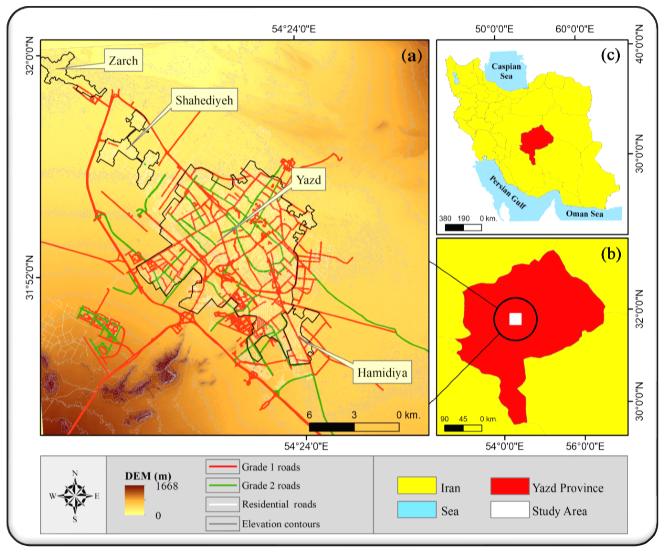
2.1. Study Area
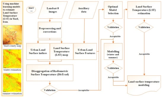
2.2. Methodology
2.2.1. Input Data: Satellite Images
2.2.2. Disaggregation of Radiometric Surface Temperature (DisTrad)
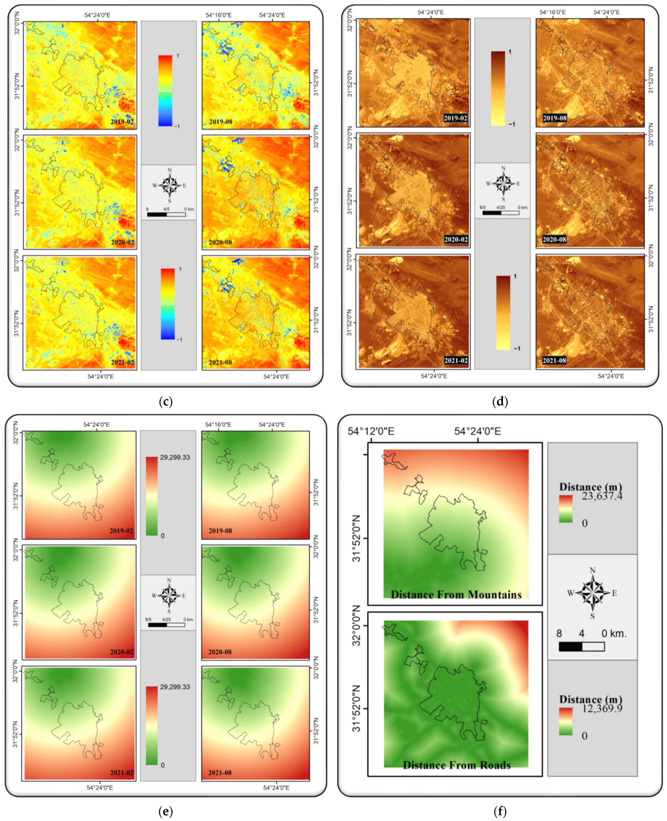
2.2.3. Land Surface Parameters
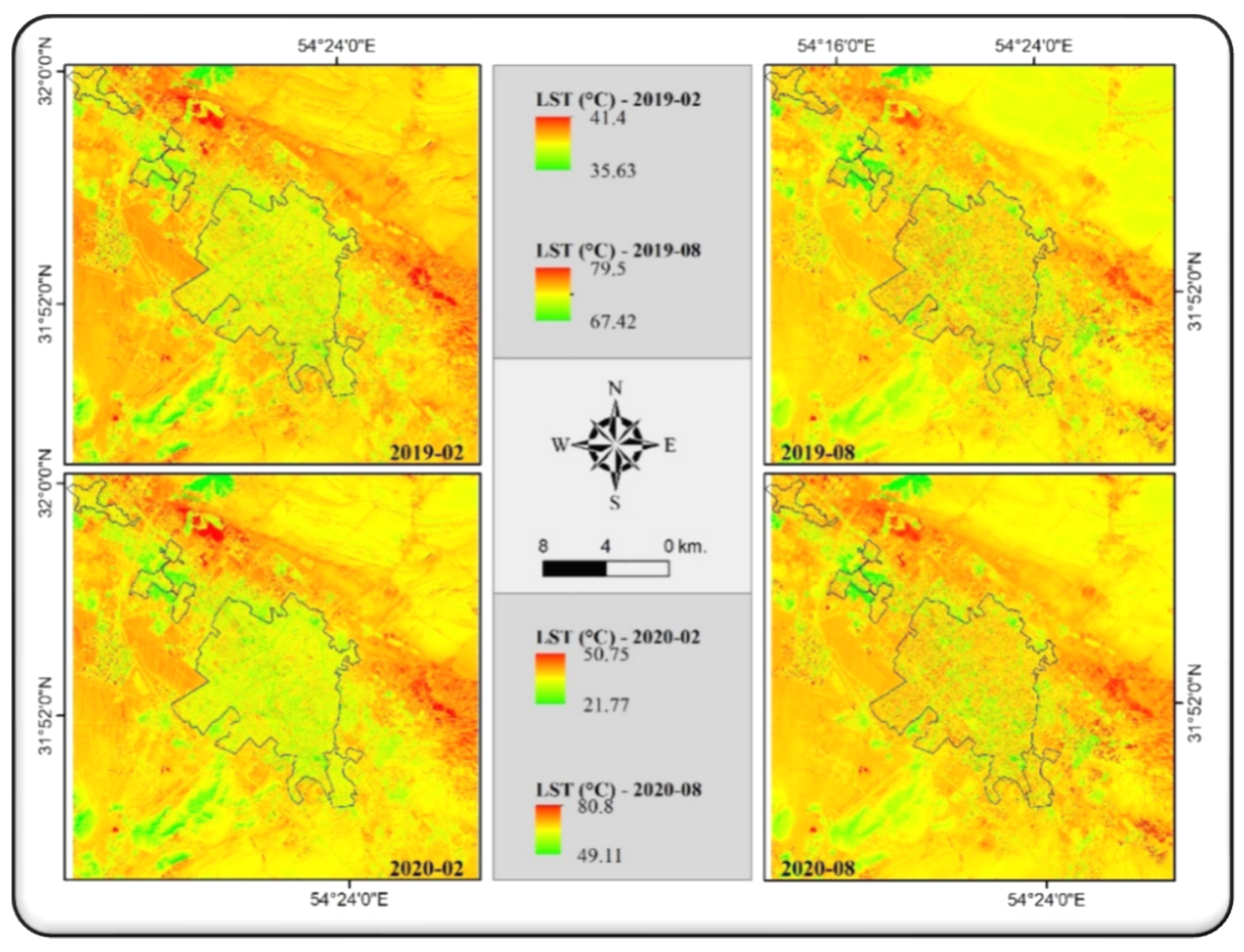
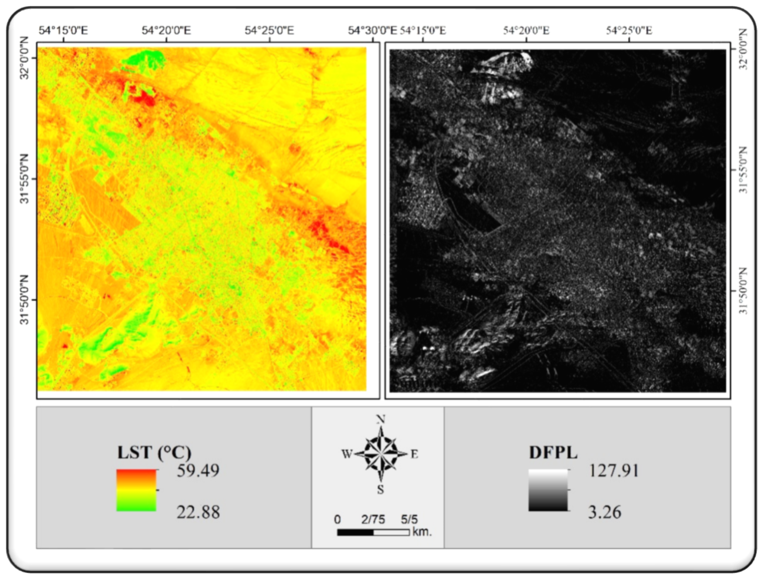
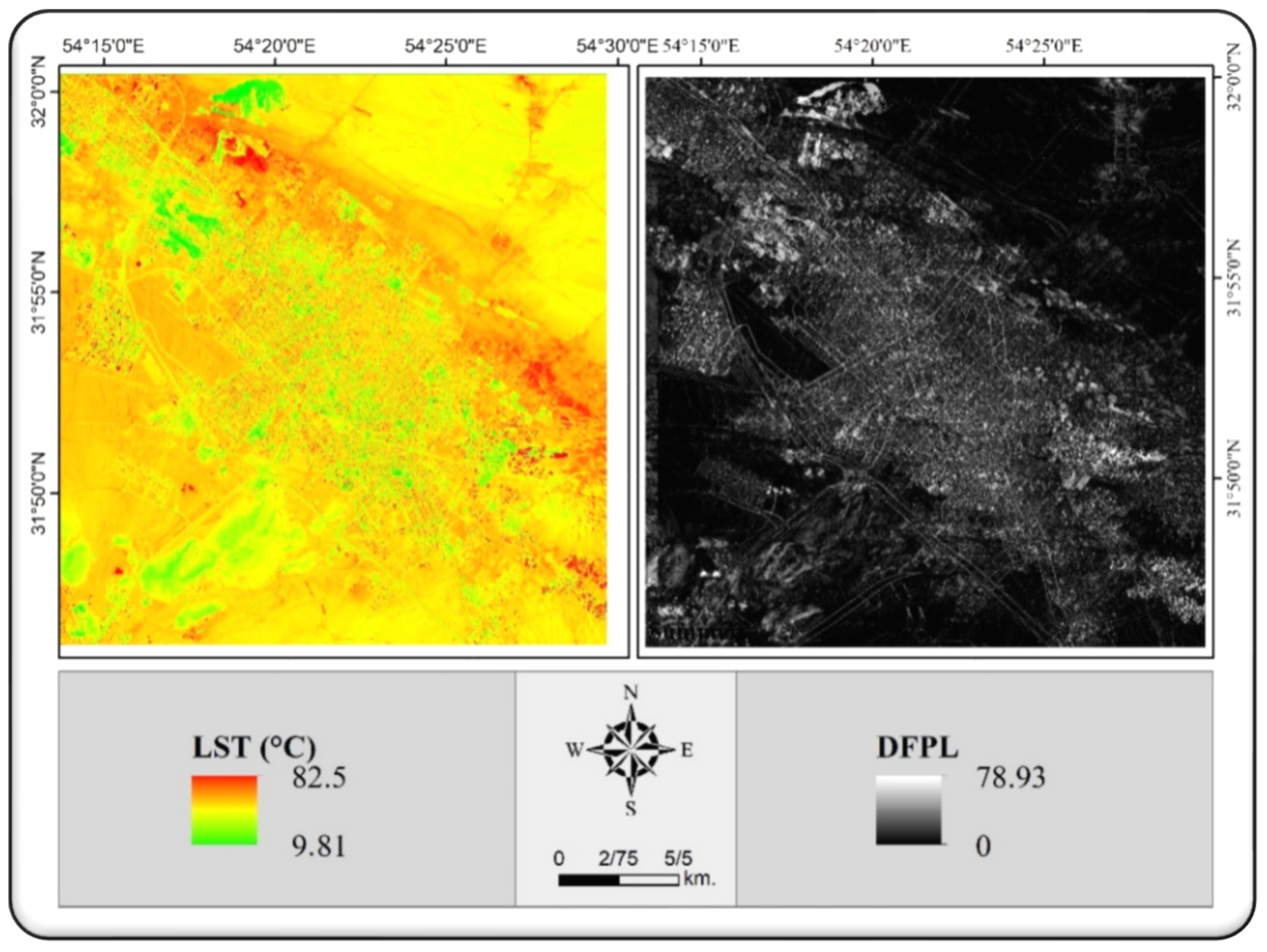
Calculation of Land Surface Temperature (LST)
Calculation of Urban Land Surface Features
- Albedo index
- Normalized Difference Built-up Index (NDBI)
- Normalized Difference Bareness Index (NDBaI)
- Elevation by Digital Elevation Map (DEM)
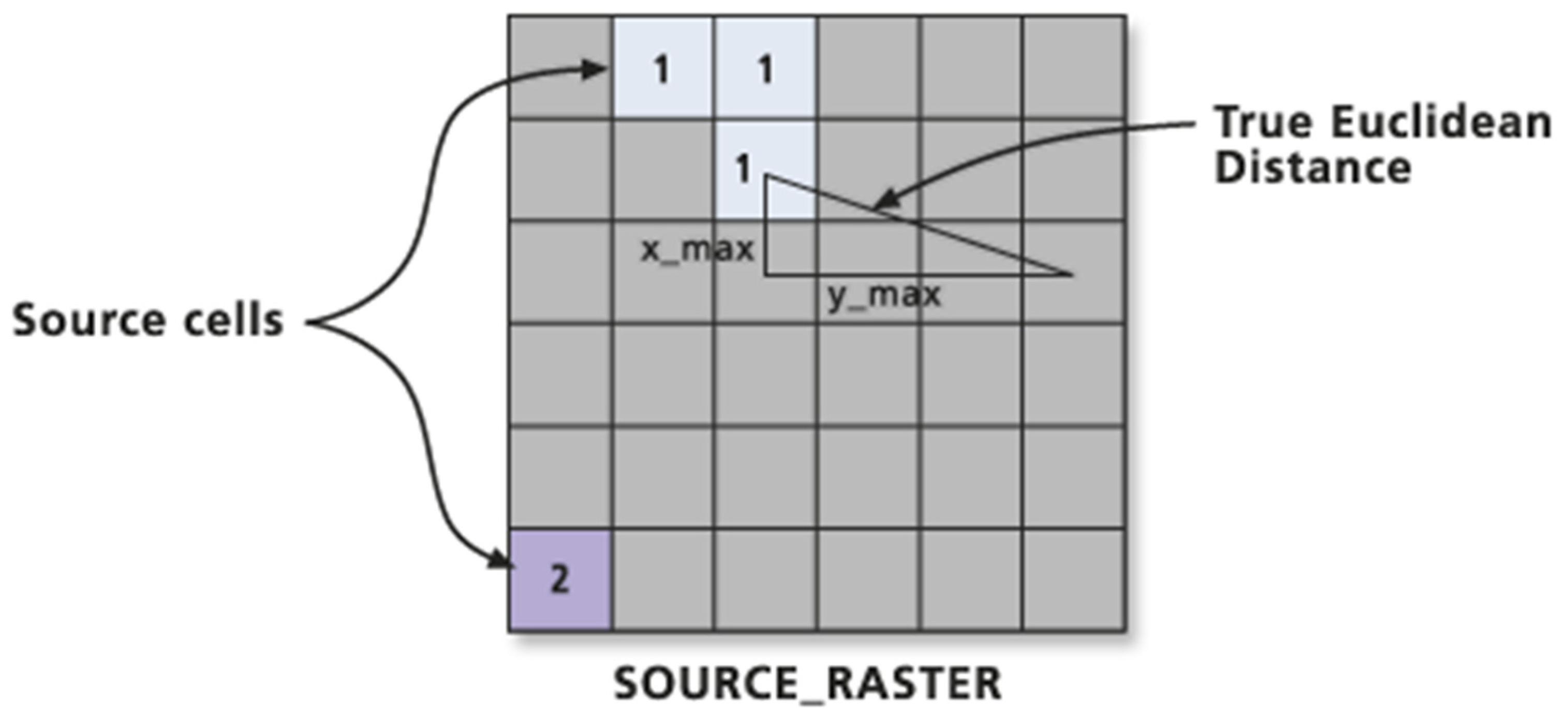
- Distances
SHapley Additive exPlanation (SHAP)
2.2.4. Optimal Model Selection
3. Results
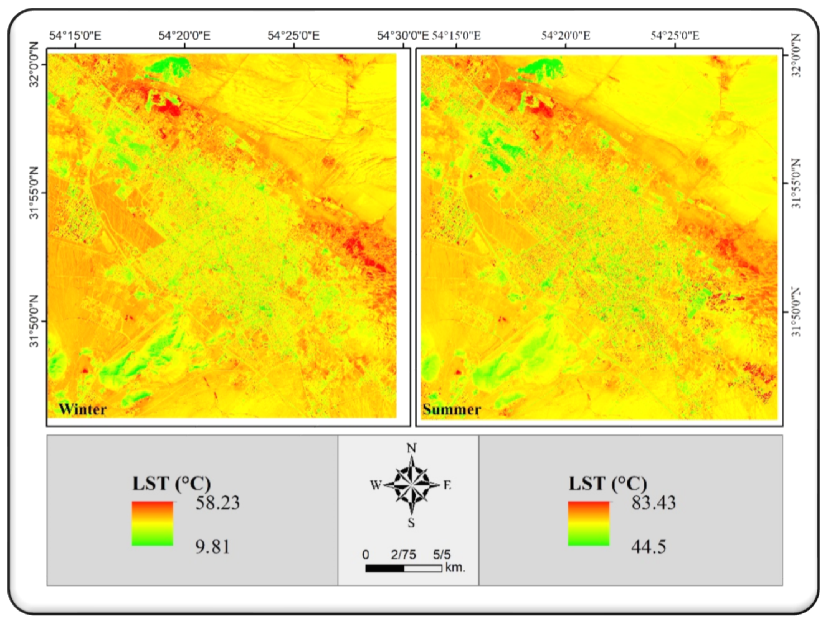
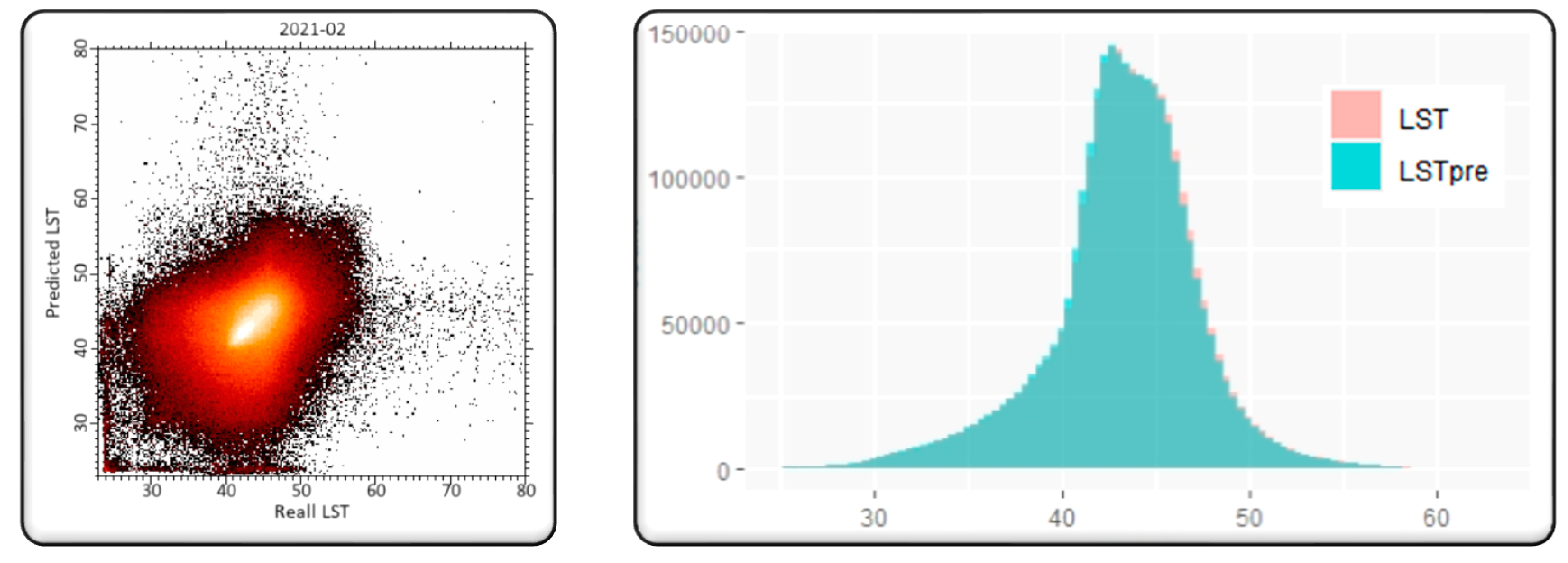
3.1. Validation of LST Maps
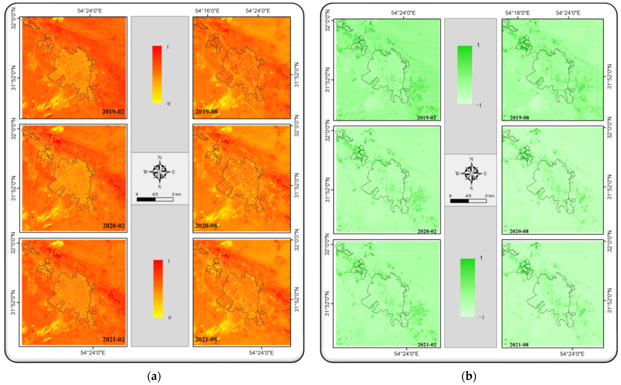
3.2. Model Input Data
3.3. Data Frame Creation, Test and Selection of the Optimum Model
3.4. Modeling of the LST
4. Discussion
5. Conclusions
- Assessing ground surface temperature using machine learning models: the GBM algorithm outperforms the other machine learning models for LST estimation, given its highest accuracy. Due to the high accuracy and the ability to use complex data such as spectral indices, machine learning models can be used to estimate LST in areas where thermal data are limited.
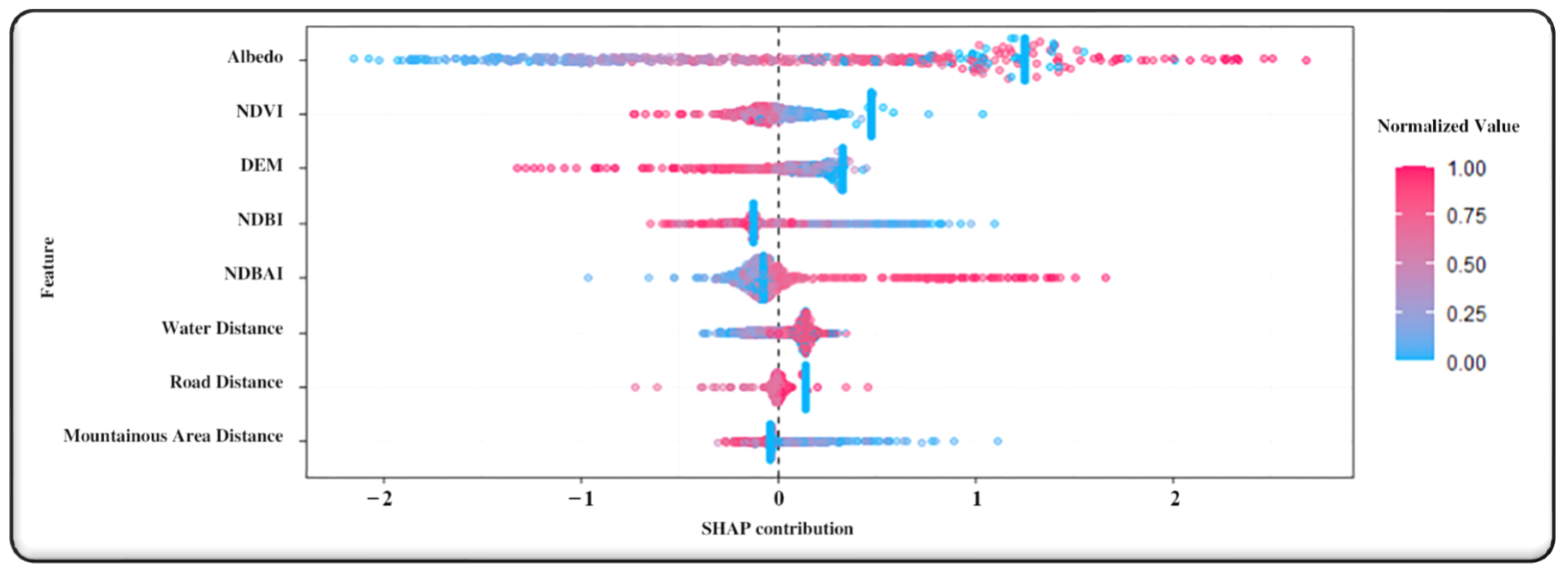
- Effect of environmental factors in determining Earth’s surface temperature: albedo exerts a significant impact on LST, with an importance of 80.30% and 72.74% in summer and winter seasons, respectively. NDVI is the second most important factor in determining LST, accounting for 11.27% and 17.21%, correspondingly. The other six ground surface features investigated have an importance of ~5% in LST for both seasons.
- Ability to estimate temperature at different spatial scales: spectral indices and machine learning algorithms can be used to estimate LST on a large spatial scale. But for smaller scales, improved and adaptive methods may be needed.
- The use of spectral indices in time analysis: by considering different spectral indices in different seasons, it is possible to conduct temporal analyses of LST and examine patterns and seasonal changes. These analyses provide a better understanding of the temperature dynamics of the study areas.
Author Contributions
Funding
Data Availability Statement
Conflicts of Interest
References
- Tong, D.; Chu, J.; Han, Q.; Liu, X. How land finance drives urban expansion under fiscal pressure: Evidence from Chinese cities. Land 2022, 11, 253. [Google Scholar] [CrossRef]
- Liu, X.; Kong, M.; Tong, D.; Zeng, X.; Lai, Y. Property rights and adjustment for sustainable development during post-productivist transitions in China. Land Use Policy 2022, 122, 106379. [Google Scholar] [CrossRef]
- Li, J.; Wang, Z.; Wu, X.; Xu, C.-Y.; Guo, S.; Chen, X. Toward monitoring short-term droughts using a novel daily scale, standardized antecedent precipitation evapotranspiration index. J. Hydrometeorol. 2020, 21, 891–908. [Google Scholar] [CrossRef]
- Wu, X.; Guo, S.; Qian, S.; Wang, Z.; Lai, C.; Li, J.; Liu, P. Long-range precipitation forecast based on multipole and preceding fluctuations of sea surface temperature. Int. J. Climatol. 2022, 42, 8024–8039. [Google Scholar] [CrossRef]
- Oke, T.R. The energetic basis of the urban heat island. Q. J. R. Meteorol. Soc. 1982, 108, 1–24. [Google Scholar] [CrossRef]
- Taha, H. Urban climates and heat islands: Albedo, evapotranspiration, and anthropogenic heat. Energy Build. 1997, 25, 99–103. [Google Scholar] [CrossRef]
- Rizwan, A.M.; Dennis, L.Y.; Chunho, L. A review on the generation, determination and mitigation of Urban Heat Island. J. Environ. Sci. 2008, 20, 120–128. [Google Scholar] [CrossRef]
- Grimmond, S.U. Urbanization and global environmental change: Local effects of urban warming. Geogr. J. 2007, 173, 83–88. [Google Scholar] [CrossRef]
- Kikegawa, Y.; Genchi, Y.; Yoshikado, H.; Kondo, H. Development of a numerical simulation system toward comprehensive assessments of urban warming countermeasures including their impacts upon the urban buildings’ energy-demands. Appl. Energy 2003, 76, 449–466. [Google Scholar] [CrossRef]
- Plocoste, T.; Jacoby-Koaly, S.; Molinié, J.; Petit, R. Evidence of the effect of an urban heat island on air quality near a landfill. Urban Clim. 2014, 10, 745–757. [Google Scholar] [CrossRef]
- Meineke, E.K.; Dunn, R.R.; Frank, S.D. Early pest development and loss of biological control are associated with urban warming. Biol. Lett. 2014, 10, 20140586. [Google Scholar] [CrossRef] [PubMed]
- Şimşek, Ç.K.; Ödül, H. A method proposal for monitoring the microclimatic change in an urban area. Sustain. Cities Soc. 2019, 46, 101407. [Google Scholar] [CrossRef]
- Liu, L.; Li, Z.; Fu, X.; Liu, X.; Li, Z.; Zheng, W. Impact of power on uneven development: Evaluating built-up area changes in Chengdu based on NPP-VIIRS images (2015–2019). Land 2022, 11, 489. [Google Scholar] [CrossRef]
- Alavipanah, S.K. Thermal Remote Sensing and Its Application in the Earth Sciences; University of Tehran Press: Tehran, Iran, 2006; pp. 903–964. [Google Scholar]
- Mansourmoghaddam, M.; Naghipur, N.; Rousta, I.; Alavipanah, S.K.; Olafsson, H.; Ali, A.A. Quantifying the Effects of Green-Town Development on Land Surface Temperatures (LST)(A Case Study at Karizland (Karizboom), Yazd, Iran). Land 2023, 12, 885. [Google Scholar] [CrossRef]
- Jia, B.; Zhou, G. Estimation of global karst carbon sink from 1950s to 2050s using response surface methodology. Geo-Spat. Inf. Sci. 2023, 1–18. [Google Scholar] [CrossRef]
- Zhang, S.; Bai, X.; Zhao, C.; Tan, Q.; Luo, G.; Wang, J.; Li, Q.; Wu, L.; Chen, F.; Li, C. Global CO2 consumption by silicate rock chemical weathering: Its past and future. Earth’s Future 2021, 9, e2020EF001938. [Google Scholar] [CrossRef]
- Wang, P.; Yu, P.; Lu, J.; Zhang, Y. The mediation effect of land surface temperature in the relationship between land use-cover change and energy consumption under seasonal variations. J. Clean. Prod. 2022, 340, 130804. [Google Scholar] [CrossRef]
- Kazemi Garajeh, M.; Salmani, B.; Zare Naghadehi, S.; Valipoori Goodarzi, H.; Khasraei, A. An integrated approach of remote sensing and geospatial analysis for modeling and predicting the impacts of climate change on food security. Sci. Rep. 2023, 13, 1057. [Google Scholar] [CrossRef]
- Osborne, P.E.; Alvares-Sanches, T. Quantifying how landscape composition and configuration affect urban land surface temperatures using machine learning and neutral landscapes. Comput. Environ. Urban Syst. 2019, 76, 80–90. [Google Scholar] [CrossRef]
- Quattrochi, D.A.; Luvall, J.C. Thermal infrared remote sensing for analysis of landscape ecological processes: Methods and applications. Landsc. Ecol. 1999, 14, 577–598. [Google Scholar] [CrossRef]
- Li, W.; Wang, W.; Sun, R.; Li, M.; Liu, H.; Shi, Y.; Zhu, D.; Li, J.; Ma, L.; Fu, S. Influence of nitrogen addition on the functional diversity and biomass of fine roots in warm-temperate and subtropical forests. For. Ecol. Manag. 2023, 545, 121309. [Google Scholar] [CrossRef]
- Lin, J.; Wei, K.; Guan, Z. Exploring the connection between morphological characteristic of built-up areas and surface heat islands based on MSPA. Urban Clim. 2024, 53, 101764. [Google Scholar] [CrossRef]
- Tran, D.X.; Pla, F.; Latorre-Carmona, P.; Myint, S.W.; Caetano, M.; Kieu, H.V. Characterizing the relationship between land use land cover change and land surface temperature. ISPRS J. Photogramm. Remote Sens. 2017, 124, 119–132. [Google Scholar] [CrossRef]
- Shang, K.; Xu, L.; Liu, X.; Yin, Z.; Liu, Z.; Li, X.; Yin, L.; Zheng, W. Study of urban heat island effect in Hangzhou metropolitan area based on SW-TES algorithm and image dichotomous model. SAGE Open 2023, 13, 21582440231208851. [Google Scholar] [CrossRef]
- Collas, L.; Green, R.E.; Ross, A.; Wastell, J.H.; Balmford, A. Urban development, land sharing and land sparing: The importance of considering restoration. J. Appl. Ecol. 2017, 54, 1865–1873. [Google Scholar] [CrossRef]
- Stott, I.; Soga, M.; Inger, R.; Gaston, K.J. Land sparing is crucial for urban ecosystem services. Front. Ecol. Environ. 2015, 13, 387–393. [Google Scholar] [CrossRef]
- Amiri, R.; Weng, Q.; Alimohammadi, A.; Alavipanah, S.K. Spatial–temporal dynamics of land surface temperature in relation to fractional vegetation cover and land use/cover in the Tabriz urban area, Iran. Remote Sens. Environ. 2009, 113, 2606–2617. [Google Scholar] [CrossRef]
- Shang, Y.; Song, K.; Lai, F.; Lyu, L.; Liu, G.; Fang, C.; Hou, J.; Qiang, S.; Yu, X.; Wen, Z. Remote sensing of fluorescent humification levels and its potential environmental linkages in lakes across China. Water Res. 2023, 230, 119540. [Google Scholar] [CrossRef]
- Mansourmoghaddam, M.; Ghafarian Malamiri, H.R.; Rousta, I.; Olafsson, H.; Zhang, H. Assessment of Palm Jumeirah Island’s Construction Effects on the Surrounding Water Quality and Surface Temperatures during 2001–2020. Water 2022, 14, 634. [Google Scholar] [CrossRef]
- Wen, Z.; Wang, Q.; Ma, Y.; Jacinthe, P.A.; Liu, G.; Li, S.; Shang, Y.; Tao, H.; Fang, C.; Lyu, L. Remote estimates of suspended particulate matter in global lakes using machine learning models. Int. Soil Water Conserv. Res. 2024, 12, 200–216. [Google Scholar] [CrossRef]
- Li, R.; Zhu, G.; Lu, S.; Sang, L.; Meng, G.; Chen, L.; Jiao, Y.; Wang, Q. Effects of Urbanization on the water cycle in the Shiyang River Basin: Based on stable isotope method. Hydrol. Earth Syst. Sci. Discuss. 2023, 2023, 4437–4452. [Google Scholar] [CrossRef]
- Grimmond, C. Progress in measuring and observing the urban atmosphere. Theor. Appl. Climatol. 2006, 84, 3–22. [Google Scholar] [CrossRef]
- Piringer, M.; Grimmond, C.S.B.; Joffre, S.M.; Mestayer, P.; Middleton, D.; Rotach, M.; Baklanov, A.; De Ridder, K.; Ferreira, J.; Guilloteau, E. Investigating the surface energy balance in urban areas–recent advances and future needs. Water Air Soil Pollut. Focus 2002, 2, 1–16. [Google Scholar] [CrossRef]
- Jiang, J.; Tian, G. Analysis of the impact of land use/land cover change on land surface temperature with remote sensing. Procedia Environ. Sci. 2010, 2, 571–575. [Google Scholar] [CrossRef]
- Peng, X.; Wu, W.; Zheng, Y.; Sun, J.; Hu, T.; Wang, P. Correlation analysis of land surface temperature and topographic elements in Hangzhou, China. Sci. Rep. 2020, 10, 1–16. [Google Scholar] [CrossRef] [PubMed]
- Alavipanah, S.K.; Hashemi Darrehbadami, S.; Kazemzadeh, A. Spatial-Temporal Analysis of Urban Heat-Island of Mashhad City due to Land Use/Cover Change and Expansion. Geogr. Urban Plan. Res. 2015, 3, 1–17. [Google Scholar]
- IBM. What is Machine Learning? Available online: https://www.ibm.com/cloud/learn/machine-learning (accessed on 19 January 2024).
- Ozturk, D. Urban growth simulation of Atakum (Samsun, Turkey) using cellular automata-Markov chain and multi-layer perceptron-Markov chain models. Remote Sens. 2015, 7, 5918–5950. [Google Scholar] [CrossRef]
- Musa, S.I.; Hashim, M.; Reba, M.N.M. A review of geospatial-based urban growth models and modelling initiatives. Geocarto Int. 2017, 32, 813–833. [Google Scholar] [CrossRef]
- Li, Q.; Zheng, H. Prediction of summer daytime land surface temperature in urban environments based on machine learning. Sustain. Cities Soc. 2023, 97, 104732. [Google Scholar] [CrossRef]
- Peng, J.; Ma, J.; Liu, Q.; Liu, Y.; Li, Y.; Yue, Y. Spatial-temporal change of land surface temperature across 285 cities in China: An urban-rural contrast perspective. Sci. Total Environ. 2018, 635, 487–497. [Google Scholar] [CrossRef]
- Mansourmoghaddam, M.; Rousta, I.; Zamani, M.S.; Mokhtari, M.H.; Karimi Firozjaei, M.; Alavipanah, S.K. Investigating And Modeling the Effect of The Composition and Arrangement of The Landscapes of Yazd City on The Land Surface Temperature Using Machine Learning and Landsat-8 and Sentinel-2 Data. Iran. J. Remote Sens. GIS 2022, 15, 1–26. [Google Scholar]
- CustomWeather. Climate & Weather Averages in Yazd, Iran. Available online: https://www.timeanddate.com/weather/iran/yazd/climate (accessed on 1 February 2022).
- Adler-Golden, S.M.; Matthew, M.W.; Bernstein, L.S.; Levine, R.Y.; Berk, A.; Richtsmeier, S.C.; Acharya, P.K.; Anderson, G.P.; Felde, J.W.; Gardner, J. Atmospheric correction for shortwave spectral imagery based on MODTRAN4. In Proceedings of the Imaging Spectrometry V, Denver, CO, USA, 19–21 July 1999; pp. 61–69. [Google Scholar]
- Berk, A.; Bernstein, L.; Anderson, G.; Acharya, P.; Robertson, D.; Chetwynd, J.; Adler-Golden, S. MODTRAN cloud and multiple scattering upgrades with application to AVIRIS. Remote Sens. Environ. 1998, 65, 367–375. [Google Scholar] [CrossRef]
- Berk, A.; Bernstein, L.; Robertson, D. MODTRAN: A Moderate Resolution Model for LOWTRAN 7; Final Report; Geophysics Laboratory: Las Vegas, NV, USA, 1989. [Google Scholar]
- Matthew, M.W.; Adler-Golden, S.M.; Berk, A.; Richtsmeier, S.C.; Levine, R.Y.; Bernstein, L.S.; Acharya, P.K.; Anderson, G.P.; Felde, G.W.; Hoke, M.L. Status of atmospheric correction using a MODTRAN4-based algorithm. In Proceedings of the Algorithms for Multispectral, Hyperspectral, and Ultraspectral Imagery VI, Orlando, FL, USA, 24–28 April 2000; pp. 199–207. [Google Scholar]
- Johnson, B.; Young, S.J. In-Scene Atmospheric Compensation: Application to SEBASS Data Collected at the ARM Site; Space and Environment Technology Center, the Aerospace Corporation: Segundo, CA, USA, 1998. [Google Scholar]
- Hernandez-Baquero, E.D. Characterization of the Earth’s Surface and Atmosphere from Multispectral and Hyperspectral Thermal Imagery; Air Force Inst of Tech Wright-Pattersonafb Oh School of Engineering: Dayton, OH, USA, 2000. [Google Scholar]
- Essa, W.; Verbeiren, B.; van der Kwast, J.; Van de Voorde, T.; Batelaan, O. Evaluation of the DisTrad thermal sharpening methodology for urban areas. Int. J. Appl. Earth Obs. Geoinf. 2012, 19, 163–172. [Google Scholar] [CrossRef]
- Bindhu, V.; Narasimhan, B.; Sudheer, K. Development and verification of a non-linear disaggregation method (NL-DisTrad) to downscale MODIS land surface temperature to the spatial scale of Landsat thermal data to estimate evapotranspiration. Remote Sens. Environ. 2013, 135, 118–129. [Google Scholar] [CrossRef]
- Essa, W.; van der Kwast, J.; Verbeiren, B.; Batelaan, O. Downscaling of thermal images over urban areas using the land surface temperature–impervious percentage relationship. Int. J. Appl. Earth Obs. Geoinf. 2013, 23, 95–108. [Google Scholar] [CrossRef]
- Sara, K.; Eswar, R.; Bhattacharya, B.K. The Utility of Simpler Spatial Disaggregation Models for Retrieving Land Surface Temperature at High Spatiotemporal Resolutions. IEEE Geosci. Remote Sens. Lett. 2021, 19, 1–5. [Google Scholar] [CrossRef]
- Kustas, W.P.; Norman, J.M.; Anderson, M.C.; French, A.N. Estimating subpixel surface temperatures and energy fluxes from the vegetation index–radiometric temperature relationship. Remote Sens. Environ. 2003, 85, 429–440. [Google Scholar] [CrossRef]
- Wu, J.; Xia, L.; Chan, T.O.; Awange, J.; Zhong, B. Downscaling land surface temperature: A framework based on geographically and temporally neural network weighted autoregressive model with spatio-temporal fused scaling factors. ISPRS J. Photogramm. Remote Sens. 2022, 187, 259–272. [Google Scholar] [CrossRef]
- Ranagalage, M.; Estoque, R.C.; Handayani, H.H.; Zhang, X.; Morimoto, T.; Tadono, T.; Murayama, Y. Relation between urban volume and land surface temperature: A comparative study of planned and traditional cities in Japan. Sustainability 2018, 10, 2366. [Google Scholar] [CrossRef]
- Bokaie, M.; Zarkesh, M.K.; Arasteh, P.D.; Hosseini, A. Assessment of urban heat island based on the relationship between land surface temperature and land use/land cover in Tehran. Sustain. Cities Soc. 2016, 23, 94–104. [Google Scholar] [CrossRef]
- Avdan, U.; Jovanovska, G. Algorithm for automated mapping of land surface temperature using LANDSAT 8 satellite data. J. Sens. 2016, 2016, 1480307. [Google Scholar] [CrossRef]
- Dos Santos, A.R.; de Oliveira, F.S.; da Silva, A.G.; Gleriani, J.M.; Gonçalves, W.; Moreira, G.L.; Silva, F.G.; Branco, E.R.F.; Moura, M.M.; da Silva, R.G. Spatial and temporal distribution of urban heat islands. Sci. Total Environ. 2017, 605, 946–956. [Google Scholar] [CrossRef] [PubMed]
- Estoque, R.C.; Pontius Jr, R.G.; Murayama, Y.; Hou, H.; Thapa, R.B.; Lasco, R.D.; Villar, M.A. Simultaneous comparison and assessment of eight remotely sensed maps of Philippine forests. Int. J. Appl. Earth Obs. Geoinf. 2018, 67, 123–134. [Google Scholar] [CrossRef]
- Sultana, S.; Satyanarayana, A. Urban heat island intensity during winter over metropolitan cities of India using remote-sensing techniques: Impact of urbanization. Int. J. Remote Sens. 2018, 39, 6692–6730. [Google Scholar] [CrossRef]
- Ziaul, S.; Pal, S. Image based surface temperature extraction and trend detection in an urban area of West Bengal, India. J. Environ. Geogr. 2016, 9, 13–25. [Google Scholar] [CrossRef]
- Rousta, I.; Sarif, M.O.; Gupta, R.D.; Olafsson, H.; Ranagalage, M.; Murayama, Y.; Zhang, H.; Mushore, T.D. Spatiotemporal analysis of land use/land cover and its effects on surface urban heat island using Landsat data: A case study of Metropolitan City Tehran (1988–2018). Sustainability 2018, 10, 4433. [Google Scholar] [CrossRef]
- LANDSAT 8 Data Users Handbook; Department of the Interior US Geological Survey: Reston, VA, USA, 2015.
- Liang, S. Narrowband to broadband conversions of land surface albedo I: Algorithms. Remote Sens. Environ. 2001, 76, 213–238. [Google Scholar] [CrossRef]
- Rouse, J.W.; Haas, R.H.; Schell, J.A.; Deering, D.W. Monitoring vegetation systems in the Great Plains with ERTS. NASA Spec. Publ. 1974, 351, 309. [Google Scholar]
- Zha, Y.; Gao, J.; Ni, S. Use of normalized difference built-up index in automatically mapping urban areas from TM imagery. Int. J. Remote Sens. 2003, 24, 583–594. [Google Scholar] [CrossRef]
- Oke, T.R. Boundary Layer Climates; Routledge: London, UK, 2002. [Google Scholar]
- Wang, W.; Liang, S.; Meyers, T. Validating MODIS land surface temperature products using long-term nighttime ground measurements. Remote Sens. Environ. 2008, 112, 623–635. [Google Scholar] [CrossRef]
- Jimenez-Munoz, J.C.; Cristobal, J.; Sobrino, J.A.; Sòria, G.; Ninyerola, M.; Pons, X. Revision of the single-channel algorithm for land surface temperature retrieval from Landsat thermal-infrared data. IEEE Trans. Geosci. Remote Sens. 2008, 47, 339–349. [Google Scholar] [CrossRef]
- Zhao, F.; Wu, H.; Zhu, S.; Zeng, H.; Zhao, Z.; Yang, X.; Zhang, S. Material stock analysis of urban road from nighttime light data based on a bottom-up approach. Environ. Res. 2023, 228, 115902. [Google Scholar] [CrossRef] [PubMed]
- Smith, R. The Heat Budget of the Earth’s Surface Deduced from Space; Yale Center for Earth Observation: New Haven, CT, USA, 2010. [Google Scholar]
- Li, X.; Zhou, Y.; Asrar, G.R.; Imhoff, M.; Li, X. The surface urban heat island response to urban expansion: A panel analysis for the conterminous United States. Sci. Total Environ. 2017, 605, 426–435. [Google Scholar] [CrossRef] [PubMed]
- Weng, Q.; Yang, S. Urban air pollution patterns, land use, and thermal landscape: An examination of the linkage using GIS. Environ. Monit. Assess. 2006, 117, 463–489. [Google Scholar] [CrossRef] [PubMed]
- Ya’acob, N.; Azize, A.B.M.; Mahmon, N.A.; Yusof, A.L.; Azmi, N.F.; Mustafa, N. Temporal forest change detection and forest health assessment using Remote Sensing. IOP Conf. Ser. Earth Environ. Sci. 2014, 19, 012017. [Google Scholar]
- Rasul, A.; Balzter, H.; Ibrahim, G.R.F.; Hameed, H.M.; Wheeler, J.; Adamu, B.; Ibrahim, S.; Najmaddin, P.M. Applying built-up and bare-soil indices from Landsat 8 to cities in dry climates. Land 2018, 7, 81. [Google Scholar] [CrossRef]
- As-Syakur, A.R.; Adnyana, I.W.S.; Arthana, I.W.; Nuarsa, I.W. Enhanced built-up and bareness index (EBBI) for mapping built-up and bare land in an urban area. Remote Sens. 2012, 4, 2957–2970. [Google Scholar] [CrossRef]
- esri. Understanding Euclidean distance analysis. Available online: https://desktop.arcgis.com/en/arcmap/latest/tools/spatial-analyst-toolbox/understanding-euclidean-distance-analysis.htm#ESRI_SECTION1_29048F6D811B40D0A0B7E2BA0F36E92E (accessed on 30 August 2022).
- Xu, H. A study on information extraction of water body with the modified normalized difference water index (MNDWI). J. Remote Sens. 2005, 9, 595. [Google Scholar]
- Shapley, L.S. A value for n-person games. In Contributions to the Theory of Games II; Kuhn, H., Tucker, A., Eds.; Princeton University Press: Princeton, NJ, USA, 1953. [Google Scholar]
- Gramegna, A.; Giudici, P. Why to buy insurance? an explainable artificial intelligence approach. Risks 2020, 8, 137. [Google Scholar] [CrossRef]
- Joseph, A. Shapley regressions: A framework for statistical inference on machine learning models. arXiv 2019, arXiv:1903.04209v1. [Google Scholar] [CrossRef]
- Lundberg, S.M.; Erion, G.G.; Lee, S.-I. Consistent individualized feature attribution for tree ensembles. arXiv 2018, arXiv:1802.03888. [Google Scholar]
- h2o. SHAP Summary Plot. Available online: https://docs.h2o.ai/h2o/latest-stable/h2o-r/docs/reference/h2o.shap_summary_plot.html (accessed on 7 January 2024).
- h2o. H2O AutoML: Automatic Machine Learning. Available online: https://docs.h2o.ai/h2o/latest-stable/h2o-docs/automl.html (accessed on 13 January 2024).
- Breiman, L. Random forests. Mach. Learn. 2001, 45, 5–32. [Google Scholar] [CrossRef]
- Geurts, P.; Ernst, D.; Wehenkel, L. Extremely randomized trees. Mach. Learn. 2006, 63, 3–42. [Google Scholar] [CrossRef]
- Friedman, J.H. Greedy function approximation: A gradient boosting machine. Ann. Stat. 2001, 29, 1189–1232. [Google Scholar] [CrossRef]
- McCullagh, P.; Nelder, J. Generalized Linear Models; CRC Press: Boca Raton, FL, USA, 1989. [Google Scholar]
- Sill, J.; Takács, G.; Mackey, L.; Lin, D. Feature-weighted linear stacking. arXiv 2009, arXiv:0911.0460. [Google Scholar]
- LeCun, Y.; Bengio, Y.; Hinton, G. Deep learning. Nature 2015, 521, 436–444. [Google Scholar] [CrossRef]
- Vakayil, A.; Joseph, R.; Mak, S. SPlit: Split a dataset for training and testing. R Package Version 2021, 1. [Google Scholar]
- Joseph, V.R. Optimal ratio for data splitting. Stat. Anal. Data Min. ASA Data Sci. J. 2022, 15, 531–538. [Google Scholar] [CrossRef]
- DeWitt, D.J.; Naughton, J.F.; Schneider, D.F. Parallel Sorting on a Shared-Nothing Architecture Using Probabilistic Splitting; University of Wisconsin-Madison Department of Computer Sciences: Madison, WI, USA, 1991. [Google Scholar]
- Chen, J.; Lu, S. Improved parameterized set splitting algorithms: A probabilistic approach. Algorithmica 2009, 54, 472–489. [Google Scholar] [CrossRef]
- Li, Z.-L.; Tang, B.-H.; Wu, H.; Ren, H.; Yan, G.; Wan, Z.; Trigo, I.F.; Sobrino, J.A. Satellite-derived land surface temperature: Current status and perspectives. Remote Sens. Environ. 2013, 131, 14–37. [Google Scholar] [CrossRef]
- Xu, J.; Zhou, G.; Su, S.; Cao, Q.; Tian, Z. The development of a rigorous model for bathymetric mapping from multispectral satellite-images. Remote Sens. 2022, 14, 2495. [Google Scholar] [CrossRef]
- Wan, R.; Wang, P.; Wang, X.; Yao, X.; Dai, X. Modeling wetland aboveground biomass in the Poyang Lake National Nature Reserve using machine learning algorithms and Landsat-8 imagery. J. Appl. Remote Sens. 2018, 12, 046029. [Google Scholar] [CrossRef]
- Zhou, G.; Su, S.; Xu, J.; Tian, Z.; Cao, Q. Bathymetry Retrieval From Spaceborne Multispectral Subsurface Reflectance. IEEE J. Sel. Top. Appl. Earth Obs. Remote Sens. 2023, 16, 2547–2558. [Google Scholar] [CrossRef]
- Singh, R.K.; Singh, P.; Drews, M.; Kumar, P.; Singh, H.; Gupta, A.K.; Govil, H.; Kaur, A.; Kumar, M. A machine learning-based classification of LANDSAT images to map land use and land cover of India. Remote Sens. Appl. Soc. Environ. 2021, 24, 100624. [Google Scholar] [CrossRef]
- Elith, J.; Leathwick, J.R.; Hastie, T. A working guide to boosted regression trees. J. Anim. Ecol. 2008, 77, 802–813. [Google Scholar] [CrossRef]
- Wu, J.; Zhong, B.; Tian, S.; Yang, A.; Wu, J. Downscaling of urban land surface temperature based on multi-factor geographically weighted regression. IEEE J. Sel. Top. Appl. Earth Obs. Remote Sens. 2019, 12, 2897–2911. [Google Scholar] [CrossRef]
- Ghosh, A.; Joshi, P. Hyperspectral imagery for disaggregation of land surface temperature with selected regression algorithms over different land use land cover scenes. ISPRS J. Photogramm. Remote Sens. 2014, 96, 76–93. [Google Scholar] [CrossRef]
- Liu, F.; Wang, X.; Sun, F.; Wang, H.; Wu, L.; Zhang, X.; Liu, W.; Che, H. Correction of Overestimation in Observed Land Surface Temperatures Based on Machine Learning Models. J. Clim. 2022, 35, 5359–5377. [Google Scholar] [CrossRef]
- Keramitsoglou, I.; Kiranoudis, C.T.; Weng, Q. Downscaling geostationary land surface temperature imagery for urban analysis. IEEE Geosci. Remote Sens. Lett. 2013, 10, 1253–1257. [Google Scholar] [CrossRef]
- Han, D.; An, H.; Cai, H.; Wang, F.; Xu, X.; Qiao, Z.; Jia, K.; Sun, Z.; An, Y. How do 2D/3D urban landscapes impact diurnal land surface temperature: Insights from block scale and machine learning algorithms. Sustain. Cities Soc. 2023, 99, 104933. [Google Scholar] [CrossRef]
- Khan, M.; Qasim, M.; Tahir, A.A.; Farooqi, A. Machine learning-based assessment and simulation of land use modification effects on seasonal and annual land surface temperature variations. Heliyon 2023, 9, e23043. [Google Scholar] [CrossRef] [PubMed]
- Luo, J.; Wang, Y.; Li, G. The innovation effect of administrative hierarchy on intercity connection: The machine learning of twin cities. J. Innov. Knowl. 2023, 8, 100293. [Google Scholar] [CrossRef]
- Ali, S.; Eum, H.-I.; Cho, J.; Dan, L.; Khan, F.; Dairaku, K.; Shrestha, M.L.; Hwang, S.; Nasim, W.; Khan, I.A. Assessment of climate extremes in future projections downscaled by multiple statistical downscaling methods over Pakistan. Atmos. Res. 2019, 222, 114–133. [Google Scholar] [CrossRef]
- Hussain, S.; Mubeen, M.; Nasim, W.; Mumtaz, F.; Abdo, H.G.; Mostafazadeh, R.; Fahad, S. Assessment of future prediction of urban growth and climate change in district Multan, Pakistan using CA-Markov method. Urban Clim. 2024, 53, 101766. [Google Scholar] [CrossRef]
- NASA. Albedo Values. Available online: https://mynasadata.larc.nasa.gov/basic-page/albedo-values (accessed on 19 January 2024).
- Julien, Y.; Sobrino, J.A.; Verhoef, W. Changes in land surface temperatures and NDVI values over Europe between 1982 and 1999. Remote Sens. Environ. 2006, 103, 43–55. [Google Scholar] [CrossRef]
- Kaufmann, R.K.; Zhou, L.; Myneni, R.; Tucker, C.J.; Slayback, D.; Shabanov, N.; Pinzon, J. The effect of vegetation on surface temperature: A statistical analysis of NDVI and climate data. Geophys. Res. Lett. 2003, 30. [Google Scholar] [CrossRef]
- Sun, D.; Kafatos, M. Note on the NDVI-LST relationship and the use of temperature-related drought indices over North America. Geophys. Res. Lett. 2007, 34. [Google Scholar] [CrossRef]
- Mansourmoghaddam, M.; Rousta, I.; Zamani, M.; Mokhtari, M.H.; Karimi Firozjaei, M.; Alavipanah, S.K. Study and prediction of land surface temperature changes of Yazd city: Assessing the proximity and changes of land cover. J. RS GIS Nat. Resour. 2022, 12, 1–5. [Google Scholar]
- Guha, S.; Govil, H.; Gill, N.; Dey, A. A long-term seasonal analysis on the relationship between LST and NDBI using Landsat data. Quat. Int. 2021, 575, 249–258. [Google Scholar] [CrossRef]
- Huang, H.; Huang, J.; Wu, Y.; Zhuo, W.; Song, J.; Li, X.; Li, L.; Su, W.; Ma, H.; Liang, S. The improved winter wheat yield estimation by assimilating GLASS LAI into a crop growth model with the proposed Bayesian posterior-based ensemble Kalman filter. IEEE Trans. Geosci. Remote Sens. 2023, 61, 1–18. [Google Scholar] [CrossRef]
- Zheng, H.; Fan, X.; Bo, W.; Yang, X.; Tjahjadi, T.; Jin, S. A multiscale point-supervised network for counting maize tassels in the wild. Plant Phenomics 2023, 5, 0100. [Google Scholar] [CrossRef] [PubMed]
- Wang, W.; Samat, A.; Abuduwaili, J.; Ge, Y. Quantifying the influences of land surface parameters on LST variations based on GeoDetector model in Syr Darya Basin, Central Asia. J. Arid Environ. 2021, 186, 104415. [Google Scholar] [CrossRef]
- Nardino, M.; Laruccia, N. Land Use Changes in a Peri-Urban Area and Consequences on the Urban Heat Island. Climate 2019, 7, 133. [Google Scholar] [CrossRef]
- Muthiah, K.; Mathivanan, M.; Duraisekaran, E. Dynamics of urban sprawl on the peri-urban landscape and its relationship with urban heat island in Chennai Metropolitan Area, India. Arab. J. Geosci. 2022, 15, 1694. [Google Scholar] [CrossRef]
- Jato-Espino, D. Spatiotemporal statistical analysis of the Urban Heat Island effect in a Mediterranean region. Sustain. Cities Soc. 2019, 46, 101427. [Google Scholar] [CrossRef]


| Satellite/Sensor | Spatial Resolution (m) | Date/Hour (GMT) | Image ID | Cloud Cover (%) |
|---|---|---|---|---|
| Landsat-8/OLI | 30 | 2019-02-07 06:56:42 | LC08_L1TP_162038_20190207_20200829_02_T1 | 31.0 |
| 2019-08-18 06:57:05 | LC08_L1TP_162038_20190818_20200827_02_T1 | 0.0 | ||
| 2020-02-12 06:56:59 | LC08_L1TP_162038_20200210_20200823_02_T1 | 36.4 | ||
| 2020-08-18 06:56:59 | LC08_L1TP_162038_20200820_20200905_02_T1 | 27.0 | ||
| 2021-02-12 06:57:01 | LC08_L1TP_162038_20210212_20210302_02_T1 | 19.0 | ||
| 2021-08-23 06:57:07 | LC08_L1TP_162038_20210823_20210831_02_T1 | 22.4 |
| Sensor | Band | K1 [W/(m2·sr·µm)] | K2 [K] |
|---|---|---|---|
| TIRS | 10 | 774.8 | 1321 |
| LST Date | RMSE (°C) |
|---|---|
| 2019-02-07 | 2.08 |
| 2019-08-18 | 4.001 |
| 2020-02-12 | 2.97 |
| 2020-08-18 | 2.01 |
| Rank | Season | Model ID | RMSE (°C) | MAE (°C) | RMSLE (°C) |
|---|---|---|---|---|---|
| 1 | Summer | GBM_4_AutoML_1_20220802_231417 | 0.32 | 0.17 | 0.00 |
| Winter | GBM_1_AutoML_1_20220803_104005 | 0.27 | 0.14 | 0.01 | |
| 2 | Summer | GBM_3_AutoML_1_20220802_231417 | 0.33 | 0.16 | 0.00 |
| Winter | DeepLearning_1_AutoML_1_20220803_104005 | 0.32 | 0.16 | 0.01 | |
| 3 | Summer | GBM_5_AutoML_1_20220802_231417 | 0.34 | 0.17 | 0.00 |
| Winter | StackedEnsemble_BestOfFamily_3_AutoML_1_20220803_104005 | 0.34 | 0.22 | 0.01 | |
| 4 | Summer | GBM_2_AutoML_1_20220802_231417 | 0.34 | 0.17 | 0.00 |
| Winter | StackedEnsemble_AllModels_2_AutoML_1_20220803_104005 | 0.34 | 0.22 | 0.01 | |
| 5 | Summer | GBM_1_AutoML_1_20220802_231417 | 0.34 | 0.16 | 0.00 |
| Winter | StackedEnsemble_AllModels_3_AutoML_1_20220803_104005 | 0.34 | 0.22 | 0.01 | |
| 6 | Summer | DRF_1_AutoML_1_20220802_231417 | 0.34 | 0.16 | 0.00 |
| Winter | StackedEnsemble_AllModels_1_AutoML_1_20220803_104005 | 0.35 | 0.22 | 0.01 | |
| 7 | Summer | XRT_1_AutoML_1_20220802_231417 | 0.35 | 0.17 | 0.00 |
| Winter | StackedEnsemble_BestOfFamily_1_AutoML_1_20220803_104005 | 0.35 | 0.22 | 0.01 | |
| 8 | Summer | DeepLearning_1_AutoML_1_20220802_231417 | 0.39 | 0.19 | 0.01 |
| Winter | StackedEnsemble_BestOfFamily_2_AutoML_1_20220803_104005 | 0.35 | 0.22 | 0.01 | |
| 9 | Summer | GBM_grid_1_AutoML_1_20220802_231417_model_1 | 0.43 | 0.26 | 0.01 |
| Winter | DRF_1_AutoML_1_20220803_104005 | 0.39 | 0.22 | 0.01 | |
| 10 | Summer | DeepLearning_grid_1_AutoML_1_20220802_231417_model_3 | 0.48 | 0.27 | 0.01 |
| Winter | XRT_1_AutoML_1_20220803_104005 | 0.44 | 0.25 | 0.01 | |
| 11 | Summer | DeepLearning_grid_1_AutoML_1_20220802_231417_model_2 | 0.48 | 0.26 | 0.01 |
| Winter | GBM_3_AutoML_1_20220803_104005 | 0.60 | 0.42 | 0.01 | |
| 12 | Summer | DeepLearning_grid_1_AutoML_1_20220802_231417_model_1 | 0.51 | 0.29 | 0.01 |
| Winter | GBM_2_AutoML_1_20220803_104005 | 0.60 | 0.42 | 0.01 | |
| 13 | Summer | StackedEnsemble_AllModels_4_AutoML_1_20220802_231417 | 0.64 | 0.52 | 0.01 |
| Winter | GBM_4_AutoML_1_20220803_104005 | 0.67 | 0.47 | 0.02 | |
| 14 | Summer | StackedEnsemble_AllModels_3_AutoML_1_20220802_231417 | 0.65 | 0.53 | 0.01 |
| Winter | GLM_1_AutoML_1_20220803_104005 | 0.68 | 0.51 | 0.02 | |
| 15 | Summer | StackedEnsemble_AllModels_2_AutoML_1_20220802_231417 | 0.65 | 0.53 | 0.01 |
| Winter | DeepLearning_grid_1_AutoML_1_20220803_104005_model_1 | 0.82 | 0.63 | 0.02 | |
| 16 | Summer | StackedEnsemble_AllModels_1_AutoML_1_20220802_231417 | 0.65 | 0.53 | 0.01 |
| Winter | GBM_5_AutoML_1_20220803_104005 | 1.27 | 0.90 | 0.03 | |
| 17 | Summer | StackedEnsemble_BestOfFamily_3_AutoML_1_20220802_231417 | 0.65 | 0.54 | 0.01 |
| Winter | GBM_grid_1_AutoML_1_20220803_104005_model_1 | 1.98 | 1.31 | 0.05 |
| Rank | Season | Variable | Importance (%) | Scaled Importance |
|---|---|---|---|---|
| 1 | Summer | Albedo | 80.30 | 1.00000 |
| Winter | Albedo | 72.74 | 1.00000 | |
| 2 | Summer | NDVI | 11.27 | 0.12769 |
| Winter | NDVI | 17.21 | 0.21058 | |
| 3 | Summer | NDBAI | 3.23 | 0.00260 |
| Winter | NDBI | 4.45 | 0.00548 | |
| 4 | Summer | NDBI | 1.16 | 0.00183 |
| Winter | NDBAI | 1.44 | 0.00534 | |
| 5 | Summer | DEM | 1.02 | 0.00021 |
| Winter | Water Distance | 1.09 | 0.00109 | |
| 6 | Summer | Road Distance | 1.01 | 0.00009 |
| Winter | Mountainous Area Distance | 1.04 | 0.00046 | |
| 7 | Summer | Water Distance | 1.01 | 0.00007 |
| Winter | Road Distance | 1.02 | 0.00024 | |
| 8 | Summer | Mountainous Area Distance | 1.00 | 0.00003 |
| Winter | DEM | 1.01 | 0.00018 |
| Index (°C) | Winter | Summer |
|---|---|---|
| Mean | 3.03 | 2.858 |
| STDEV | 3.280 | 3.484 |
| Index | Winter (°C) | Summer (°C) |
|---|---|---|
| MAE | 3.559 | 3.358 |
| RMSE | 5.247 | 5.296 |
| RMSLE | 0.152 | 0.128 |
Disclaimer/Publisher’s Note: The statements, opinions and data contained in all publications are solely those of the individual author(s) and contributor(s) and not of MDPI and/or the editor(s). MDPI and/or the editor(s) disclaim responsibility for any injury to people or property resulting from any ideas, methods, instructions or products referred to in the content. |
© 2024 by the authors. Licensee MDPI, Basel, Switzerland. This article is an open access article distributed under the terms and conditions of the Creative Commons Attribution (CC BY) license (https://creativecommons.org/licenses/by/4.0/).
Share and Cite
Mansourmoghaddam, M.; Rousta, I.; Ghafarian Malamiri, H.; Sadeghnejad, M.; Krzyszczak, J.; Ferreira, C.S.S. Modeling and Estimating the Land Surface Temperature (LST) Using Remote Sensing and Machine Learning (Case Study: Yazd, Iran). Remote Sens. 2024, 16, 454. https://doi.org/10.3390/rs16030454
Mansourmoghaddam M, Rousta I, Ghafarian Malamiri H, Sadeghnejad M, Krzyszczak J, Ferreira CSS. Modeling and Estimating the Land Surface Temperature (LST) Using Remote Sensing and Machine Learning (Case Study: Yazd, Iran). Remote Sensing. 2024; 16(3):454. https://doi.org/10.3390/rs16030454
Chicago/Turabian StyleMansourmoghaddam, Mohammad, Iman Rousta, Hamidreza Ghafarian Malamiri, Mostafa Sadeghnejad, Jaromir Krzyszczak, and Carla Sofia Santos Ferreira. 2024. "Modeling and Estimating the Land Surface Temperature (LST) Using Remote Sensing and Machine Learning (Case Study: Yazd, Iran)" Remote Sensing 16, no. 3: 454. https://doi.org/10.3390/rs16030454
APA StyleMansourmoghaddam, M., Rousta, I., Ghafarian Malamiri, H., Sadeghnejad, M., Krzyszczak, J., & Ferreira, C. S. S. (2024). Modeling and Estimating the Land Surface Temperature (LST) Using Remote Sensing and Machine Learning (Case Study: Yazd, Iran). Remote Sensing, 16(3), 454. https://doi.org/10.3390/rs16030454