Abstract
Coastal wetlands play an important carbon sequestration role in China’s “carbon peaking” and “carbon neutrality” goals. Monitoring aboveground biomass (AGB) is crucial for wetland management. Satellite remote sensing enables efficient retrieval of AGB. However, a variety of statistical models can be used for biomass inversion, depending on factors such as the vegetation type and inversion method. In this study, Landsat 8 Operational Land Imager (OLI) images were preprocessed in the study area through radiation calibration and atmospheric correction for modeling. In terms of model selection, 13 different models, including the univariate regression model, multiple regression model, and machine learning regression model, were compared in terms of their accuracy in estimating the biomass of various wetland vegetation types under their respective optimal parameters. The findings revealed that: (1) the regression models varied across vegetation types, with the accuracy of the biomass estimates decreasing in the order of Scirpus spp. > Spartina alterniflora > Phragmites australis; (2) overall modeling, without distinguishing vegetation types, addressed the challenges of limited samples availability and sampling difficulty. Among them, the random forest regression model outperformed the others in estimating wet and dry AGB with R2 values of 0.806 and 0.839, respectively. (3) Comparatively, individual modeling of vegetation types can better reflect the biomass of each wetland vegetation type, especially the dry AGB of Scirpus spp., whose R2 and RMSE values increased by 0.248 and 11.470 g/m2, respectively. This study evaluates the impact of coastal saltmarsh vegetation types on biomass estimation, providing insights into biomass dynamics and valuable support for wetland conservation and restoration, with potential contributions to global habitat assessment models and international policies like the 30x30 Conservation Agenda.
1. Introduction
Coastal wetland vegetation biomass carbon is a significant component of carbon storage in coastal saltmarshes [1,2,3]. Through the process of photosynthesis, wetland vegetation can convert inorganic carbon in wetland ecosystems into organic carbon, which plays a crucial role in the carbon cycle of saltmarsh wetlands in China [4,5]. However, there are variations and differences in the biomass carbon of coastal wetland vegetation due to factors such as vegetation type, geographical location, and nutrient conditions [6,7,8]. The utilization of remote sensing images can not only effectively compensate for the limitations of accessibility and difficulties in obtaining wetland vegetation biomass samples but also integrate images for analyzing the spatial and temporal variations in biomass [9,10,11].
Remote sensing can be used to estimate the distribution and growth of wetland vegetation and other resources. A statistical model can be established between the spectral data of remote sensing images and the aboveground biomass (AGB) of vegetation, and the biomass can be quickly estimated over a large area. This method solves the problems of poor accessibility and safety concerns associated with ground surveys and the sampling of wetland vegetation biomass [12,13]. Remote sensing is widely used in the fields of vegetation resource investigation, dynamic monitoring, and biomass estimation [14,15,16]. However, unlike the remote sensing inversion of aboveground biomass in forests and farmland, wetland vegetation is affected by complex environmental factors, such as differences in underlying surface conditions [17,18]. In particular, in the Chongming Island area, wetland vegetation is significantly affected by the law of natural differentiation [10]. The east is affected mainly by seawater, whereas the west is affected mainly by the Yangtze River, resulting in high heterogeneity in wetland vegetation growth and complex spectral response processes [19]. In addition, different plants differ in their spectral, absorption, and reflection characteristics. Distinguishing wetland vegetation types for biomass remote sensing inversion may reduce the impact of spectral response differences between different vegetation types to a certain extent and improve the estimation accuracy of aboveground biomass [20]. However, it is still unclear how the biomass remote sensing inversion of multiple wetland vegetation types in the same area differs and what specific impacts distinguishing vegetation type modeling and non-distinguishing vegetation type modeling will have on the wetland vegetation biomass inversion process.
In the selection of vegetation biomass inversion models, traditional statistical models such as univariate and multiple linear regressions have been used [21]. With the development of machine learning, nonparametric machine learning methods such as the neural network (NN) regression model, support vector regression (SVR) model, and random forest (RF) regression model have shown great potential for the inversion of AGB from wetland vegetation in recent years [22,23,24,25,26]. Gao et al. [27] utilized the RF model along with the hyperspectral verification method of plots to increase the accuracy of Moderate Resolution Imaging Spectroradiometer (MODIS) images for estimating the AGB and coverage of alpine grasslands on the Qinghai–Tibet Plateau. Pecina et al. [28] used a high-resolution dataset acquired by an unmanned aerial vehicle (UAV) platform combined with the RF algorithm to estimate the AGB of coastal meadows in Estonia. Lu et al. [29] proposed a solution that combined UAV and Sentinel-2 data to successfully estimate and map the AGB of Phragmites australis in the Nandagang Wetland Reserve in Hebei Province, China, effectively solving the problem of insufficient AGB samples due to the difficulty of accessing wetlands. Prakash et al. [30] introduced a robust methodological protocol, which employs machine learning models alongside field measurements and multisensor SAR data, to achieve highly accurate and low uncertainty estimates of AGB in mangrove forests (R2 = 0.93). Statistical methods are the main methods for biomass estimation, but the choice of model depends on factors such as the study area and vegetation type. Previous research has noted variations in biomass among different wetland vegetation types [31,32,33]. However, it is unclear how modeling these types separately versus an overall model impacts biomass estimation. Currently, there is a gap in systematic research on coastal wetland biomass inversion, and the distribution pattern of wetland vegetation biomass on Chongming Island has not been determined.
From the perspective of image data sources, Landsat, Sentinel-2, MODIS, and other data have been widely used when optical satellite images are used to invert vegetation aboveground biomass [34,35,36]. Among them, Landsat images offer higher spatial resolution than MODIS images and are better suited for wetland vegetation communities with limited distribution areas [37,38,39]. While Sentinel-2 images provide even higher spatial resolution, their use in large-scale studies demands a greater volume of image data, involves significant computational effort, and is constrained by the lack of earlier historical records [40,41,42]. In contrast, Landsat data are widely preferred because of their easy accessibility and their broad and historical perspective on vegetation [43,44]. Statistical methods are the main methods used for biomass estimation via optical remote sensing images, but the choice of model depends on factors such as the study area and vegetation type.
In addition to optical data, synthetic aperture radar (SAR) and light detection and ranging (Lidar) data can enhance the accuracy of AGB estimation [45,46,47]. Zhu et al. [48] integrated SAR and UAV data to estimate the AGB of the largest artificially planted mangrove forest in China on Qi’ao Island, which could provide more detailed and accurate information for AGB estimation. Salum et al. [49] combined Lidar data and improved the inversion accuracy of mangrove biomass data. Lucas et al. [50] retrieved mangrove distribution, age, structure, and biomass parameters by combining optical and SAR data in a Malaysian reserve. While SAR has potential for mangrove biomass retrieval [51,52,53], coastal herbaceous wetland vegetation, such as P. australis and Spartina alterniflora, can be challenging to retrieve via SAR data because of their low height and weaker radar signal returns. On the other hand, Lidar has high accuracy in retrieving vegetation height but has limited availability [33,54,55]. Furthermore, obtaining ground lidar data in coastal wetlands is difficult, and large-scale monitoring via UAV data is currently challenging [56,57]. Considering the cost-effectiveness and workload involved in data processing, Landsat imagery is the superior choice for the inversion of aboveground biomass in coastal wetland vegetation.
In this study, various wetland vegetation AGB inversion models, such as univariate regression models, multiple linear regression models, and machine learning regression models, were compared based on Landsat images to explore the most suitable AGB retrieval method for each wetland vegetation type. Additionally, the impact of classification modeling on the AGB inversion of wetland vegetation was quantitatively analyzed to examine the utility of different models, spectral bands, species classification, and both parametric and nonparametric statistical methods for biomass prediction. By comprehensively comparing various vegetation types and inversion methods, this research quantitatively reveals the influence of different saltmarsh vegetation types on the remote sensing inversion of wetland AGB. Such an approach is essential for assessing wetland AGB over large areas, significantly enhancing our understanding of biomass dynamics in coastal ecosystems and providing more reliable data support for ecological monitoring and resource management.
2. Materials and Methods
2.1. Study Area
Chongming Island, located in the core area of the Yangtze River Delta, is the most well-developed tidal coastal wetland in the Yangtze River estuary. It is located northeast of Shanghai, between 31°27′00″ and 31°51′15″N and 121°09′30″ and 121°54′00″E. Surrounding three rivers and facing the sea to the east, it is influenced by both the Yangtze River and the East China Sea, and it is the world’s largest estuarine alluvial island [10]. The different types of coastal wetlands form discontinuous wetland zones, which are key areas for the biodiversity of China’s coastal region and provide a suitable growth environment for various animals and plants [19,58]. It is 80 km long from east to west and 18 km wide at its widest point from north to south, with a total area of 1411 km2. Chongming Island has beautiful natural scenery and important wetland and forest resources, such as Dongping National Forest Park, Dongtan Bird Reserve, and Xisha Wetland Park. Its development goal is to construct a world-class ecological island with management and demonstration functions.
Chongming Island currently has nearly 100 species of plants with rich biodiversity. The coastal wetland vegetation of Chongming Island belongs to the North China Plain and to the shallow-water plant wetlands in the middle and lower reaches of the Yangtze River. The coastal wetland vegetation on Chongming Island is dominated by herbaceous vegetation, including P. australis, Scirpus mariqueter, Scirpus triqueter, S. alterniflora, Miscanthus saccharifleus, Juncellus serotinus, Suaeda glauca (Bunge) Bunge, Solidago decurrens Lour., and more [59]. These species play important roles in maintaining the ecological balance of wetland ecosystems and provide habitats for various wildlife species [60,61,62]. Among them, S. alterniflora, P. australis, and Scirpus spp. are the three most important types of wetland vegetation on Chongming Island. The distribution area of other herbaceous vegetation is small and scattered, making it difficult to dominate the communities.
This study investigated the AGB of three types of wetland vegetation on Chongming Island: S. alterniflora, P. australis, and Scirpus spp. (Figure 1). Among them, Scirpus spp. are considered pioneer species of coastal wetland vegetation due to their ability to colonize and establish in areas of bare mudflats, while P. australis is a widely distributed coastal vegetation type native to Chongming Island. In contrast, S. alterniflora was originally introduced as an invasive alien species to promote siltation and land formation but has now become a dominant and problematic species in many coastal wetlands in China [63].
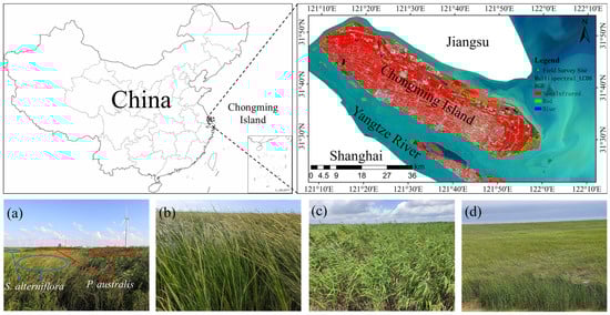
Figure 1.
Field photos of coastal wetland vegetation on Chongming Island. Panel (a) shows a field photo of the mixed growth of the native vegetation P. australis and the invasive species S. alterniflora. The red oval area represents P. australis, and the blue oval area represents S. alterniflora. Panels (b–d) correspond to the photos of the plots of S. alterniflora, P. australis, and Scirpus spp., respectively.
2.2. Data Resources
This study employed field sampling methods for investigation and sample collection. First, sample sites were selected based on uniform vegetation types, consistent growth, and continuous distributions, with each site covering an area greater than 30 × 30 m2. This approach aimed to minimize the impact of local heterogeneity and capture the spatial variability of AGB across different wetland vegetation types [19,64]. Next, biomass sampling was conducted within the selected plots. At each sample site, three 1 × 1 m2 quadrats were set up at the diagonal corners and center, and the AGB of the wetland vegetation in each quadrat was collected. All the vegetation in the sample quadrat was harvested, after which the plants were numbered separately, packed into bags, and brought back to the laboratory of the Chongming Ecological Research Institute of East China Normal University. The coordinates of the sample site, vegetation coverage, surrounding environment of the sample plot, and vegetation growth status were recorded via a handheld global positioning system (GPS) and cameras (Figure 2a,b). To obtain accurate biomass data, the vegetation collected in the field was immediately weighed and packaged, and its net wet weight was recorded with an accuracy of 0.01 g. Then, the vegetation was oven-dried at 105 °C for 30 minutes for fixation and further dried at 85 °C for more than 48 h until it reached a constant weight. Finally, the dried vegetation was weighed to obtain the dry weight of the vegetation (Figure 2c–e). The average biomass of the three sample quadrats at each sample site represented the biomass per unit area.
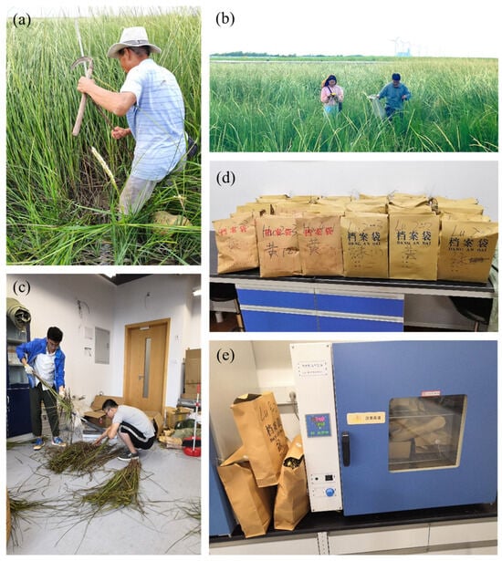
Figure 2.
(a–e) Biomass data collection process at the sample sites.
The biomass data collection process for the sample plots in the coastal wetland vegetation communities on Chongming Island was carried out from August to September 2021 (Figure S1). The data collection included 124 vegetation community sites covering the entire coastal wetland area, comprising 50 P. australis sites, 40 S. alterniflora sites, and 34 Scirpus spp. sites. The selected season for the data collection corresponds to the vigorous growth period of herbaceous vegetation and correlates well with remote sensing images. Therefore, ground data and corresponding images taken during this season were used for biomass inversion modeling.
Considering the spatial resolution of the images and the computational demands, this study selected the surface reflectance (SR) product of Landsat 8 OLI (path: 118 and row: 38) images covering Chongming Island. The Landsat 8 surface reflectance (SR) product underwent atmospheric correction using the Land Surface Reflectance Code (LaSRC) [65]. Foga et al. [66] compared various cloud removal algorithms and reported that, compared with other methods, the CFMask method, which is based on prior knowledge of physical phenomena, operates without geographical limitations and effectively removes cloud and shadow influences. Landsat 8 SR products utilize the CFMask algorithm to eliminate noise from clouds and shadows based on pixel quality and radiative saturation attributes [67]. Given the susceptibility of the Chongming Island area to cloudy and rainy weather, effective images are limited. Moreover, the AGB of wetland vegetation shows significant seasonal fluctuations but limited annual variability. Therefore, the study selected Landsat data from August to September for the years 2020 to 2022, along with ground biomass data collected from 124 vegetation community sites across Chongming Island [19]. Ultimately, the Landsat image from August 16, 2020, was chosen as the remote sensing data source for ground biomass inversion. The spatial resolution of the Landsat image is 30 m, with spectral bands including blue, green, red, near infrared, and short-wave infrared bands at 1640 nm and 2130 nm. Six original spectral and ten spectral indices of the Landsat image were extracted for use in the model (Table 1). The normalized difference vegetation index (NDVI), widely used for monitoring vegetation health and density, is sensitive to vegetation presence [68]. The soil-adjusted vegetation index (SAVI) minimizes soil interference, enabling effective differentiation of vegetation from other land cover types [69]. The ratio vegetation index (RVI) is highly sensitive to green vegetation, providing a simple measure of vegetation cover [70]. The normalized difference water indices at 1640 nm (NDWI1640) and 2130 nm (NDWI2130) effectively detect leaf water content, reflecting moisture variations, with distinct spectral bands and varying sensitivities to vegetation types and environmental conditions [71,72]. The enhanced vegetation index (EVI) is particularly responsive to canopy structure changes, making it suitable for monitoring biomass in dense vegetation [73]. The difference vegetation index (DVI) is well correlated with biomass in low-coverage areas and is commonly used for ecological monitoring [74]. The perpendicular vegetation index (PVI) captures vegetation structural information, useful for estimating biophysical parameters [75,76]. The normalized difference senescent vegetation index (NDSVI) [77,78,79] and normalized difference residue index (NDRI) [80,81] help mitigate the effects of vegetation senescence, providing insight into late-stage growth phases. These indices collectively enable precise monitoring of vegetation dynamics, with each serving a distinct purpose to enhance the accuracy of biomass estimation.

Table 1.
Spectral indices calculation formula used in biomass inversion.
2.3. Methods
This study used biomass survey data and satellite images to extract spectral information for corresponding locations. The SR product of the Landsat 8 OLI was selected for this study. The preprocessing steps for this study included the following: cloud and shadow removal using the CFMask algorithm to ensure data clarity; and data normalization, where all spectral variables were scaled using min-max normalization. This step ensured comparability and prevented potential bias in the machine learning models due to differing magnitudes of the variables. Following these preprocessing steps, feature selection was performed to identify spectral bands and indices that were significantly correlated with biomass while remaining mutually independent, thus ensuring the inclusion of only relevant and non-redundant features. A test of significance was conducted on the six original spectral bands and ten spectral indices, and the spectral variables that were both significantly correlated with biomass and independent of each other were selected for biomass estimation. To comprehensively reveal the impact of vegetation type on the inversion of wetland AGB, this study constructed optimal biomass inversion models for different vegetation types and performed an overall biomass inversion without distinguishing between vegetation types. This approach allows for a thorough consideration of the differences in the radiation transfer processes among various vegetation types, enabling a quantitative analysis of their effects on AGB inversion. Thirteen regression models, including seven univariate models, stepwise multiple linear regression models, and five machine learning models, were compared for P. australis, S. alterniflora, Scirpus spp., and saltmarsh wetland vegetation. The optimal AGB model was chosen for each wetland vegetation type, considering the distinction between wetland vegetation types. The impacts of individual modeling of vegetation types and overall modeling without distinguishing vegetation types on biomass estimation were assessed (Figure 3). All analyses were conducted using MATLAB 2019b software [82,83,84].
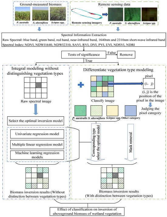
Figure 3.
Illustration of AGB inversion with and without distinguishing vegetation types.
2.3.1. Univariate Regression Model
For correlation analysis, the Pearson coefficient was used to describe the correlation between the spectral data and AGB. The Pearson coefficient reflects the correlation direction and degree between two sets of variables, and the calculation formula is as follows:
In Formula (1), is the Pearson correlation coefficient, which measures the linear correlation between two variables, and . and represent sample values in each group of variables, and represent the mean values of each group of variables. n represents the number of samples. The positive and negative values of , respectively, represent whether the two sets of variables are positively or negatively correlated. The range of r is between −1 and 1, and the closer is to 1, the higher the correlation between the variables; a value of 0 indicates no correlation [85,86,87].
Based on the correlation analysis, spectral data that were significantly and independently correlated with biomass were selected for regression modeling. Univariate models provide a straightforward approach to analyzing the direct relationships between biomass and various variable characteristics, enabling the rapid identification of appropriate fitting models [84]. Therefore, this study initially selected seven commonly used functional model forms, including linear regression and polynomial regression, for univariate regression inversion. To analyze the relationships between AGB and the spectral information of P. australis, S. alterniflora, Scirpus spp., and saltmarsh vegetation overall, seven univariate regression models were selected for the inversion of wetland vegetation AGB, including linear models, quadratic models, cubic models, power function models, exponential models, logarithmic models, and S-curve models (Table 2).
Table 2.
Calculation formula of univariate regression models.
2.3.2. Multiple Linear Regression Model
The stepwise regression model combines the forward selection and backward elimination methods, iteratively adding or removing variables based on their significance in explaining the variation of the dependent variable [88,89]. The stepwise regression method is particularly useful when dealing with large datasets with many predictors, as it can help to automatically select the most important variables for the model and exclude any variables that are irrelevant or redundant, reducing the risk of overfitting and improving the accuracy and efficiency of the model [90]. In this study, a total of 16 original spectral and spectral features were selected. Thus, the stepwise multiple linear regression method was used to establish a multivariate linear regression model between the spectral data and AGB.
2.3.3. Machine Learning Regression Models
Machine learning regression models are effective at performing nonparametric estimations and can efficiently handle high-dimensional feature data. Given the multitude of spectral features in this study, it is challenging to parameterize AGB estimation using a single spectral feature. Therefore, five machine learning regression models, namely, SVR, Gaussian process regression (GPR), RF regression, NN regression, and decision tree (DT) regression, were selected to estimate the AGB of wetland vegetation.
The SVR model can use kernel functions to project training data onto a new high-dimensional space (hyperplane) and adjust the prediction function through flexible boundary lines. The SVR model, which has multiple kernel functions and strong generalizability, is particularly useful for handling high-dimensional data and solving nonlinear regression problems. However, this approach is sensitive to missing data, and there is no uniform standard for kernel function selection. In this study, the initial values for key parameters were set as follows: the penalty coefficient C = 1.0, the kernel parameter γ = 0.1, and the slack variable ϵ = 0.1. Multiple kernel functions, including linear, polynomial, and Gaussian kernel functions, were evaluated to identify the most appropriate function for each wetland vegetation type. This comparison was conducted to enhance the accuracy and reliability of the SVR model.
The DT regression model is a popular and interpretable machine learning method that uses tree-based models to handle regression problems. Multiple decision rules branch outward, with leaf nodes that output predicted values. The use of the mean squared error for feature selection and tree pruning helps prevent overfitting and improve model generalizability. The DT regression model can provide a structured interpretation of the results, handling noise robustly, but it is at risk of overfitting the training data. In this study, the DT regression model was initialized with min samples split set to 2 and min samples leaf set to 1. These parameter settings allowed the model to grow fully, maximizing its capacity to capture data patterns without prematurely limiting tree depth, thereby ensuring comprehensive learning.
The RF regression model uses ensemble learning by combining multiple decision tree models for regression analysis, using the average of multiple decision trees to represent the result of RF regression. When the number of RF trees is sufficient, overfitting problems in regression analysis can be effectively avoided. The RF regression model is not sensitive to missing data and can sort the relative importance of input variables, making the results interpretable. In the RF model, the impact of varying the number of trees to specifically 100, 300, 500, and 1000 on prediction accuracy was systematically evaluated. To balance reliability and computational efficiency, this study used 500 trees for the RF regression model. However, it should be noted that the RF regression model may not fully leverage its advantages when the number of samples is small but rather when the number of features is large.
The NN regression model is inspired by biological neural networks that can learn data features automatically through instance data training without given rules, achieving regression prediction. The NN model is effective at handling nonlinear regression problems involving multiple variables and has been widely applied to estimate vegetation biomass. The complexity of the NN is determined by the number of layers, which directly affects the accuracy of the prediction. In this study, the neural network started with two layers, and additional layers were added iteratively up to a maximum of nine layers. The best-fitting configuration was then selected to construct the model.
GPR flexibly chooses suitable kernel functions for prediction based on data, and it provides probabilistic predictions, allowing for the calculation of empirical confidence intervals. GPR fits a distribution of random variable functions, assigning probability values to multiple potential fitting functions, with the mean of the probability distribution representing the most likely representation of the data. However, its applicability in high-dimensional spaces is limited. In this study, parameters such as the length scale (l = 1) of the RBF kernel and the smoothing parameter of the Matern kernel (ν = 1.5) were adjusted to optimize the model. The modeling performances of linear, square exponential, and other kernel functions were compared, and suitable kernel functions were flexibly selected for the GPR model.
2.3.4. Model Accuracy Evaluation
In this study, the 10-fold cross-validation method was employed to validate the inversion models. Specifically, 90% of the data was iteratively used for training, while the remaining 10% was reserved for validation [91]. This approach was chosen to enhance model reliability by reducing errors and minimizing the risk of overfitting, particularly in the context of a limited sample size [61]. All ground sample data were divided into 10 parts and used iteratively for model building and validation. The use of cross-validation allows for the full utilization of limited data and can help reduce overfitting of the model [91,92]. Because obtaining actual measurement data for wetland vegetation biomass is difficult and the quantity of data is limited, cross-validation was deemed suitable for this study. To evaluate the inversion accuracy of the model, performance evaluation metrics such as the mean absolute error (MAE) (Formula (2)), root mean square error (RMSE) (Formula (3)), coefficient of determination () (Formula (4)), and accuracy (Formula (5)) were chosen. A smaller MAE and RMSE indicate a smaller inversion error, while a higher and accuracy indicate a higher accuracy of the inversion model.
Note: represents the measured AGB of the i-th sample site, represents the predicted biomass of the i-th sample site, n represents the total number of sample sites, and represents the average value of measured biomass across all sample sites.
3. Results
This study employed 13 models, including univariate regression, multiple linear regression, and machine learning regression models, to estimate the aboveground biomass of vegetation through remote sensing. These models were specifically applied to different vegetation types, such as P. australis, S. alterniflora, and Scirpus spp., and the overall saltmarsh vegetation, which represented all of the species combined. The optimal models for each vegetation type were then integrated to estimate the aboveground biomass of the study area. This was compared with the results from the overall modeling approach to determine whether classification-based modeling enhanced the accuracy of remote sensing biomass estimation for coastal wetland vegetation. This study also aimed to quantify the degree of accuracy improvement and its impact across various vegetation types in coastal wetlands.
3.1. Single-Species AGB Retrieval
This study analyzed the relationships between spectral variables and AGB for different types of wetland vegetation. For P. australis, most spectral variables were significantly correlated with biomass, except for those in the blue band (Table 3). The red band showed the highest correlation with the wet biomass of P. australis, while the NDVI and RVI showed positive correlations. The NDSVI, red band, and NDVI were strongly correlated with dry biomass. Based on these findings, 15 noncollinear spectral variables were selected for modeling P. australis biomass. For S. alterniflora, the correlations between the spectral variables and biomass were consistent for both dry and wet biomass, except for the SWIR2130 band, which was significantly correlated with only wet biomass. Therefore, 11 variables were chosen for modeling the wet biomass of S. alterniflora, and the same 10 variables were used for modeling dry biomass, excluding SWIR2130. For Scirpus spp., all spectral variables, except for the near-infrared band and NDRI, were significantly correlated with both wet and dry biomass. Therefore, 14 spectral variables were chosen for the biomass inversion of Scirpus spp., excluding the near-infrared band and NDRI. The structural differences in vegetation canopies among species lead to variations in spectral responses between species. Additionally, different species types exhibit varying optical sensitivities across different models.
Table 3.
Correlations between the spectra and AGB of P. australis, S. alterniflora, and Scirpus spp.
3.1.1. P. australis AGB Inversion
This study evaluated different regression models for predicting the AGB of P. australis. When 105 univariate models for wet and dry AGB were compared separately (Table S1), the highest accuracy was achieved when the RVI was used as a cubic regression model. However, the accuracy of dry biomass prediction was generally lower than that of wet biomass prediction when univariate models were used for P. australis. For wet biomass estimation of P. australis, the stepwise multiple linear regression model was consistent with the univariate linear model. In contrast, for dry biomass estimation, the stepwise multiple linear regression model selected the NDSVI, with an R2 value of only 0.340. The performance of the stepwise multiple linear regression model was affected by the samples, leading to inferior performance compared with that of the optimal univariate linear regression model. Five machine learning models were compared for their ability to predict the AGB of P. australis. The RF model performed the best, utilizing spectral data effectively for biomass estimation (Table 4). The GPR model had slightly lower accuracy but was still viable. The DT model worked well for wet biomass but not for dry biomass. The SVR and NN models struggled to utilize spectral data effectively. Overall, the machine learning models were slightly more accurate for wet biomass than for dry biomass, which was consistent with the univariate and multiple linear regression models. The RF regression model outperformed the univariate regression models and stepwise multiple linear regression models in predicting the AGB of P. australis. However, limited measured data pose challenges for fully harnessing the advantages of some machine learning methods in nonparametric regression.
Table 4.
Remote sensing inversion accuracy of the AGB of P. australis based on machine learning models.
3.1.2. S. alterniflora AGB Inversion
The RVI outperformed the other spectral variables in the estimation of AGB under S. alterniflora. Among the seven univariate regression models tested, the RVI was the optimal spectral variable for all of the models except for the S-curve model when wet biomass was estimated and for all the models when dry biomass was estimated (as shown in Table S2). The comparison revealed that the quadratic model using the RVI achieved the best performance in estimating both the wet and dry biomass of S. alterniflora, with a slightly greater accuracy in estimating wet biomass. The stepwise multiple linear regression model for estimating the AGB of S. alterniflora included the RVI and NDVI as selected spectral variables; these two spectral variables had the highest correlation with the wet and dry biomass of S. alterniflora, which was consistent with the correlation analysis results. The stepwise multiple linear regression model for dry biomass estimates could use information from both the RVI and the NDVI, resulting in greater accuracy than that of univariate linear regression. However, for wet biomass estimation, the accuracy was between the accuracy of the RVI and the accuracy of the NDVI univariate linear regression models. This is due to the susceptibility of both stepwise multiple linear regression and univariate linear regression models to the influence of sample data [93]. During cross-validation, stepwise multiple linear regression did not always select RVI and NDVI values, resulting in lower overall accuracy than that of the RVI univariate linear regression model.
After the five machine learning regression models were compared, the RF regression model was found to perform well in estimating both the wet and dry biomass of S. alterniflora, with higher accuracy for wet biomass than dry biomass. The GPR model with a squared exponential kernel function achieved the second highest accuracy. However, the ability of the SVR, NN, and DT models to estimate the biomass of S. alterniflora was limited (Table 5). Although the RF regression model had a greater estimation accuracy for AGB than the stepwise regression model, it was lower than that of univariate models such as the RVI quadratic and cubic models. This is primarily because machine learning regression models struggle to learn the relationships among data when the amount of data is limited.
Table 5.
Remote sensing inversion accuracy of the AGB of S. alterniflora based on machine learning models.
3.1.3. Scirpus spp. AGB Inversion
The analysis revealed that the RVI and NDVI were more effective than the other spectral variables for estimating the wet biomass of Scirpus spp. Among the 98 univariate regression models, the logarithmic model based on the RVI had the highest accuracy in estimating the wet biomass of Scirpus spp. (Table S3). When the dry biomass of Scirpus spp. was estimated, the cubic regression model based on the NDVI had greater accuracy than the other univariate models did. Additionally, the R2 of the optimal model for wet biomass estimation was greater than that of the optimal model for dry biomass estimation. According to the stepwise regression model for the inversion of wet and dry biomass of the Scirpus spp., the RVI was selected from the 14 spectral variables. The inversion of dry biomass via stepwise regression was consistent with the use of the RVI for univariate linear regression. However, when inverting wet biomass, the spectral variable selected by the stepwise multiple linear regression model was the RVI, while the best spectral variable selected by the univariate linear regression model was the NDVI. The inconsistency between the stepwise multiple linear regression model and the univariate linear regression model was due to the different variables produced by tenfold cross-validation for each fold, and the RVI was selected more often than the NDVI in the stepwise multiple linear regression model.
When machine learning regression models are used for the wet and dry biomass inversion of Scirpus spp., both the RF and GPR methods can effectively invert AGB, and their inversion accuracy is better than that of the SVR, NN, and DT models. Among them, RF performed slightly better than GPR for wet biomass, while GPR performed better for dry biomass estimation (Table 6). However, the overall estimation accuracy of machine learning regression models is lower than that of univariate regression models, mainly due to the limitation of the sample size of the measured data, which makes it difficult to exploit the advantages of machine learning data processing.
Table 6.
Remote sensing inversion accuracy of the AGB of Scirpus spp. based on machine learning models.
In summary, when distinguishing wetland vegetation types for the AGB inversion of a single species, the inversion accuracy of different wetland vegetation types is ranked as follows: Scirpus spp. > S. alterniflora > P. australis. Additionally, different wetland vegetation types were suitable for different regression models. For example, P. australis RF regression models for the inversion of aboveground wet and dry biomass perform better than other models; Scirpus spp. are suitable for univariate regression models, where the logarithmic model using the RVI is the most accurate for the inversion of wet biomass and the cubic model using the NDVI is the most accurate for the inversion of dry biomass; and S. alterniflora is suitable for an RF regression model for wet biomass and a univariate regression model for dry biomass, where the RVI quadratic model has the smallest inversion error. Thus, a single approach may not be suitable for all wetland vegetation types, and it is necessary to choose an appropriate regression model and spectral index for accurate biomass estimation.
3.2. Remote Sensing Inversion of the Total AGB of Saltmarsh Vegetation
In previous studies, appropriate regression models for AGB estimation were selected separately for each type of wetland vegetation, but machine learning regression models may not perform well when the number of site samples is low. In addition, site sampling in wetlands requires considerable manpower and resources, resulting in limited sample sizes for each type of vegetation. To address these issues, an overall modeling approach was used with all available data on saltmarsh vegetation. This method efficiently utilizes site data, avoids multiple analyses and modeling, and provides a simple way to estimate aboveground wet and dry biomass for wetland vegetation.
The analysis of the correlation between the remote sensing spectral data and the AGB of saltmarsh wetland vegetation on Chongming Island revealed that there was a significant correlation (p < 0.01) between the wet biomass and all 15 spectral variables, except for the NDRI. Among these variables, the RVI had the highest correlation with wet biomass (Table 7).The dry biomass was significantly correlated (p < 0.01) with all 14 spectral variables except for the SWIR1640 band and was significantly correlated (p < 0.05) with the blue band. The EVI had the highest correlation with dry biomass. Therefore, the 15 spectral variables that were significantly correlated with the aboveground wet and dry biomass of saltmarsh wetland vegetation were selected for analysis.
Table 7.
Correlation between saltmarsh vegetation spectral and AGB.
The RVI was identified as the optimal spectral variable for estimating the aboveground wet biomass in saltmarsh vegetation, and the highest accuracy was achieved with the cubic model (Table 8). Additionally, the RVI proves to be more effective for wet biomass estimation compared with other spectral variables, while the EVI and NDVI are better suited for estimating aboveground dry biomass. Univariate regression models highlight the cubic model for the EVI as the most accurate for estimating aboveground dry biomass, with wet biomass estimation showing greater accuracy than dry biomass estimation in saltmarsh vegetation.
Table 8.
Remote sensing inversion accuracy of aboveground biomass of saltmarsh wetland vegetation based on univariate regression models.
Compared with univariate models, the stepwise multiple linear regression model, which incorporates the RVI and NDSVI, demonstrated greater accuracy in estimating aboveground wet biomass in saltmarsh vegetation. Additionally, for aboveground dry biomass estimation, the EVI and NDSVI selected by the stepwise multiple linear regression model outperformed the two univariate linear regression models, with dry biomass accuracy surpassing that of wet biomass in saltmarsh vegetation.
The RF regression model was the most effective among the five machine learning regression models for utilizing image spectral data to estimate the aboveground wet and dry biomass of saltmarsh vegetation. This method achieves the highest accuracy and has great potential in estimating aboveground wet biomass. Despite slightly lower accuracy, the GPR model performs well in estimating the AGB of saltmarsh vegetation and outperforms the univariate and stepwise models. The accuracy order for estimating aboveground wet biomass was RF > GPR > SVR > NN > DT, while for aboveground dry biomass, it was RF > GPR > NN > DT > SVR (Table 9). Furthermore, the overall modeling accuracy of the machine learning regression models for the overall AGB of saltmarsh vegetation was greater than that of the single vegetation type inversion methods. This is mainly due to the larger sample data available for overall modeling, which better leverages the advantages of machine learning nonparametric methods.
Table 9.
Remote sensing inversion accuracy of saltmarsh wetland vegetation AGB based on machine learning models.
3.3. Comparison of AGB Retrieval Results With and Without the Distinction of Wetland Vegetation Types
This study evaluated the performance of various models, including seven univariate models, stepwise multiple linear regression models, and five machine learning regression models, in predicting AGB for specific wetland vegetation types (P. australis, S. alterniflora, and Scirpus spp.) and overall saltmarsh vegetation. Optimal inversion models were obtained for each wetland vegetation type and overall saltmarsh vegetation, but there are advantages and disadvantages when distinguishing wetland vegetation types during modeling. Distinguishing vegetation types in modeling provides consistent impacts on radiation transfer due to the uniform plant structure and morphology of wetland vegetation. However, this approach may be influenced by other factors, such as underlying surfaces and limited sample sizes. Conversely, not distinguishing vegetation types allows for a large sample size, but variations in plant structure and morphology can lead to diverse effects on the radiation transfer process. This study further investigated the influence of differences in wetland vegetation types on AGB inversion by comparing results under conditions of distinguishing and not distinguishing vegetation types.
The RF regression model outperformed the other 12 models when modeling without distinguishing wetland vegetation types in terms of the accuracy of the inversion of AGB from saltmarsh vegetation. Consequently, this model was selected to predict the aboveground wet and dry biomass of saltmarsh vegetation. In contrast, when distinguishing between wetland vegetation types, optimal aboveground wet and dry biomass inversion models were selected for each wetland vegetation type, and their inversion results are presented in Table 10.
Table 10.
Comparison of the accuracy of remote sensing inversion of AGB with and without the distinction of wetland vegetation types.
In general, the difference in accuracy between distinguishing and not distinguishing wetland vegetation types was relatively small for the inversion of saltmarsh wetland vegetation wet and dry biomass. However, the accuracy of distinguishing vegetation types was slightly better than that of not distinguishing them. When distinguishing wetland vegetation types, the R2 values of the measured and fitted wet and dry biomasses could reach 0.806 and 0.839, respectively, and the inversion accuracy of type-based individual modeling was better than that of overall modeling for all three types of saltmarsh wetland vegetation.
For wet biomass, the difference in inversion accuracy between distinguishing and not distinguishing wetland vegetation types was relatively small. When modeling the wet biomass of P. australis separately, the R2 value was 0.541, which was slightly better than that of the overall model (0.537), and the difference in the RMSE between the individual and overall models was only 3.600 g/m2. Therefore, the overall modeling method can adequately invert the wet biomass of P. australis. Similarly, the inversion accuracy of the wet biomass of S. alterniflora was like that of P. australis, and the overall modeling method could be used to invert it as well. The differences in R2 and RMSE between distinguishing and not distinguishing wetland vegetation types were 0.027 and 8.262 g/m2, respectively. However, when the wet biomass of Scirpus spp. was inverted, the overall modeling method tends to overestimate low values and underestimate high values, and the difference in the RMSE between the individual and overall modeling methods is 11.412 g/m2. Therefore, the individual modeling method for estimating the wet biomass of Scirpus spp. is better than the overall modeling method and provides more accurate inversion results (Figure 4).
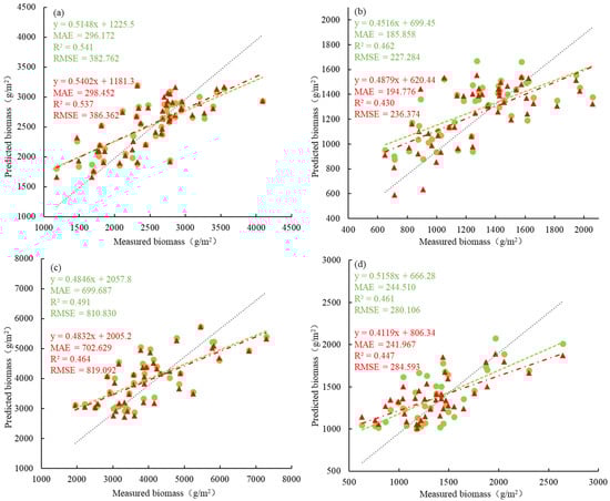
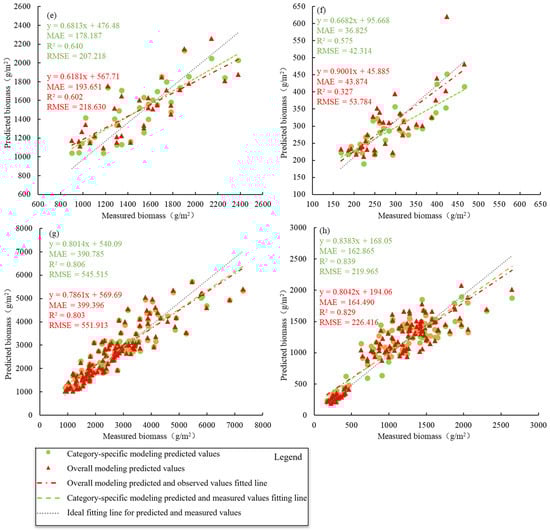
Figure 4.
Differences in AGB inversion accuracy when distinguishing and not distinguishing saltmarsh wetland vegetation types. (a) represents the wet biomass of P. australis, (b) represents the dry biomass of P. australis, (c) represents the wet biomass of S. alterniflora, (d) represents the dry biomass of S. alterniflora, (e) represents the wet biomass of Scirpus spp., (f) represents the dry biomass of Scirpus spp., (g) represents the wet biomass of saltmarsh vegetation, and (h) represents the dry biomass of saltmarsh vegetation in the figure.
The inversion accuracy between modeling individually while distinguishing wetland vegetation types and overall modeling without distinguishing vegetation types is greater for dry biomass than for wet biomass. Additionally, by distinguishing wetland vegetation types, the inversion accuracy can be improved by reducing the underestimation of high values. For the dry biomass of P. australis, there was little difference between the individual and overall modeling methods, with only small variations in R2 and RMSE of only 0.032 and 9.090 g/m2, respectively. Similarly, for the dry biomass of S. alterniflora, the differences between the individual modeling and overall modeling methods were relatively small, with differences in R2 and RMSE of only 0.014 and 4.487 g/m2, respectively. Although the overall modeling method tends to underestimate high values more than the individual modeling methods do, both methods have comparable inversion effects on the dry biomass of S. alterniflora. However, when the dry biomass of Scirpus spp. is inverted, high values are occasionally overestimated when the overall modeling method is used compared with the individual modeling methods.
In summary, univariate regression models, multiple linear regression models, and machine learning regression models were compared to estimate the aboveground wet and dry biomass of three main saltmarsh vegetation types on Chongming Island. The optimal inversion models were selected for P. australis, S. alterniflora, Scirpus spp., and all saltmarsh vegetation. The results indicated that using RF regression models for overall modeling could better fit the aboveground wet and dry biomass of wetland vegetation, with inversion results for wet biomass being superior to those for dry biomass. The inversion results for wet biomass were consistently greater than those for dry biomass, primarily because wet biomass originates from fresh vegetation with higher water content, which results in more pronounced absorption in the red wavelength band. This enhanced absorption correlates with greater inversion accuracy, with the difference in accuracy between wet and dry biomass ranging from 1.111% to 3.974%. While individual modeling with wetland vegetation types provides a better reflection of the aboveground biomass of each type, it requires multiple models and has high computational complexity. On the other hand, using the RF machine learning regression model for overall modeling without distinguishing wetland vegetation types can quickly reveal the distribution of the AGB of saltmarsh vegetation on Chongming Island with results similar to individual modeling.
3.4. Estimation of the AGB of Wetland Vegetation Under Different Models
To evaluate the impacts of different regression models on wetland vegetation AGB estimation, various models, including univariate regression, multiple linear regression, machine learning regression, and optimal model combinations for each vegetation type, were compared. The results generally revealed small differences in the inversion performances of several regression models for wet biomass. Among these models, the RF regression model estimates were similar for the combinations of various vegetation types, while the univariate regression model underestimated the S. alterniflora AGB in Beiliuyao and the stepwise regression model underestimated the Scirpus spp. AGB in Dongtan compared with the other models. A comparison of the biomass inversion of saltmarsh wetland vegetation by multiple models revealed that the RF regression model outperformed the univariate and multiple linear regression models in fitting saltmarsh vegetation AGB and reducing underestimation in some regions. Furthermore, the RF regression model, similar to the model distinguishing vegetation types, could better fit the saltmarsh wetland vegetation AGB without distinguishing vegetation types. In combination with the classification of saltmarsh wetland vegetation, species differences in AGB per unit area were also observed, with S. alterniflora having the highest biomass, followed by P. australis and Scirpus spp. The distribution of AGB per unit area of saltmarsh vegetation was consistent with the spatial classifications (as shown in Figure 5).
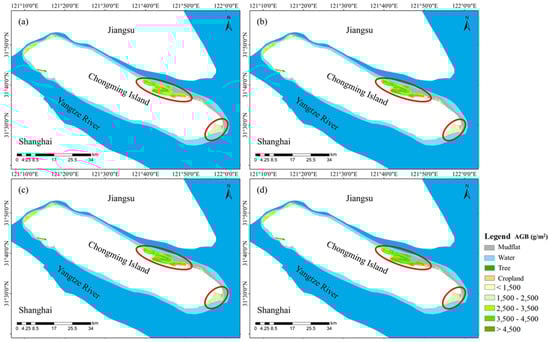
Figure 5.
Comparison of wet AGB estimates of saltmarsh vegetation. Panel (a) represents the inversions of univariate regression, (b) represents the inversions of stepwise multiple regression, (c) represents the inversions of machine learning regression, and (d) represents the results of combined inversion.
Compared with the other methods, the dry biomass inversion results revealed that the univariate regression model underestimated the S. alterniflora AGB in Beiliuyao compared to the other methods, whereas the multiple linear regression model overestimated the Scirpus spp. AGB in Dongtan compared with the other regression models (Figure 6). This is attributed to the fact that the univariate regression model has a limited ability to fit high biomass values, resulting in underestimation, while the multiple linear regression model tends to overestimate low biomass values, leading to lower fitting accuracy for low biomass values [20]. In contrast, the RF regression model effectively reduced both the overestimation of low biomass values and the underestimation of high biomass values, providing a better fit for the AGB of saltmarsh wetland vegetation. When the inversions of the RF regression model and the combined inversions for distinguishing vegetation types were compared, both methods demonstrated improved fitting of the saltmarsh vegetation AGB. However, when distinguishing saltmarsh vegetation types, the low values of S. alterniflora and P. australis and the high value of Scirpus spp. exceeded the range of sample training data and were affected by classification accuracy. Therefore, overall modeling via the RF regression model can better estimate the aboveground dry biomass of saltmarsh vegetation.
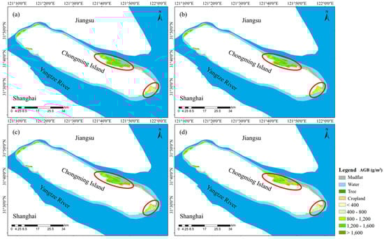
Figure 6.
Comparison of dry AGB estimates of saltmarsh vegetation. Panel (a) represents the inversions of univariate regression, (b) represents the inversions of stepwise multiple regression, (c) represents the inversions of machine learning regression, and (d) represents the results of combined inversion.
3.5. Feature Importance and Stability Analysis of the RF Regression Model
The RF regression model is effective at estimating the AGB of wetland vegetation using spectral data and can determine the relative importance of each spectral variable (Figure 7). The most crucial variable for wet biomass estimation was the RVI, followed by the NDWI2130, NDVI, and NDWI1640. NDWI2130 and NDWI1640 are ranked highly in importance because they reflect variations in vegetation water content, which is correlated with the AGB [72]. Additionally, the RVI, NDVI, and SAVI also rank high in importance as they are sensitive to differences in vegetation greenness [68,94]. Spectral indices such as the NDVI are particularly sensitive to chlorophyll content, which serves as an indicator of biomass [95,96,97]. The variables strongly correlated with wet biomass, such as the RVI, NDWI1640, and NDWI2130, are given high importance in the RF regression model. The RF regression model automatically selected suitable variables based on the data features for wetland vegetation biomass estimation.
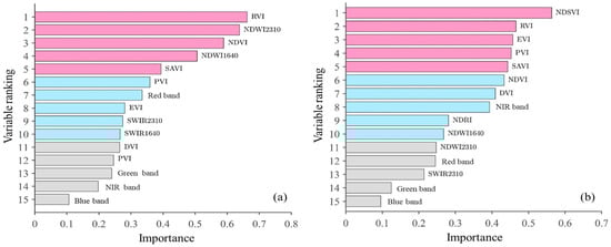
Figure 7.
Importance analysis of AGB inversion via the RF regression model. (a) is wet biomass and (b) is dry biomass.
For dry biomass estimation, the NDSVI emerged as the most important spectral variable, followed by the RVI, EVI, PVI, SAVI, NDVI, and DVI in descending order of importance. This ranking aligns with their correlation with dry biomass, with the EVI, SAVI, PVI, DVI, NDSVI, RVI, and NDVI being the top seven variables. The NDSVI is sensitive to vegetation water loss, the EVI, RVI, and SAVI reflect differences in vegetation growth, and the PVI indicates vegetation structure; all of these factors are strongly correlated with dry biomass. The RF regression model automatically selected the appropriate variables based on their correlation with biomass, ensuring reliable estimation of wetland vegetation.
The tenfold cross-validation errors between the model fittings and the measured AGB at the sample sites are shown in Figure 8. The RF regression model used in this study is stable and reliable for estimating the AGB of saltmarsh vegetation. The small fluctuation in overall sample errors indicates the model’s consistency and robustness, making it suitable for accurate AGB estimation, which is supported by the similarity in the spectral range between the sample and fitted data.
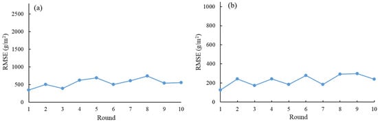
Figure 8.
Cross-validation errors of the RF regression models. Panel (a) represents the cross-validation errors of wet biomass, and (b) represents the cross-validation errors of dry biomass.
4. Discussion
4.1. Comparison of Parametric and Nonparametric Methods for Biomass Inversion
A comparison of parametric (traditional statistical) and nonparametric (machine learning) methods for estimating AGB in saltmarsh vegetation (Figure 9) revealed that the nonparametric RF regression model outperformed the parametric RVI cubic regression model and stepwise regression model for accurately estimating wet AGB (Figure 9a–c). The stepwise regression model yielded scattered predictions and a high RMSE, with overestimation in the 2500–4000 g/m2 range and underestimation in the range above 5000 g/m2, highlighting the limitations of traditional regression approaches in capturing the variability of wet biomass across different ranges. The optimal univariate regression model (the RVI cubic model) improved the fitting accuracy in the high-value area but still exhibited high dispersion between the predicted and measured results. In contrast, the nonparametric machine learning regression model effectively utilized image spectral data and achieved greater accuracy with an R2 value of 0.803, indicating its superior ability to model complex relationships between spectral indices and biomass while accounting for inherent data noise and variability. However, for dry biomass estimation, the correlation with dry weight biomass is greater than that with wet weight biomass, primarily because the association between dry matter and spectral indices is less affected by moisture content. This observation underscores the critical role of moisture as a confounding factor in wet biomass estimation, which is more effectively mitigated through machine learning approaches. The univariate regression model (EVI cubic model) showed notable variance and underestimation for high biomasses above 1800 g/m2, along with overestimation in the 800–1400 g/m2 range, resulting in limited accuracy in predictions (Figure 9d–f). Compared with the univariate model, the stepwise regression model slightly reduced the variance but still significantly underestimated high biomass values above 1800 g/m2 and performed poorly for low biomass values below 500 g/m2, even yielding some negative values. These results indicate that stepwise regression models are limited by their dependence on predefined linear relationships, making them insufficient for accounting for the nonlinear and heteroscedastic nature of biomass data in marsh ecosystems [90]. In contrast, the RF regression model demonstrated the capability to handle these nonlinearities, effectively reducing the overestimation of low dry biomass values and the underestimation of high dry biomass values, achieving an R2 value of 0.829. This performance highlights its potential for accurately estimating the dry biomass of marsh vegetation.
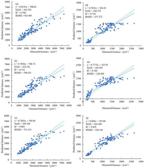
Figure 9.
Comparison of the AGB inversion results for saltmarsh vegetation. Panels (a–c) illustrate the inversion of wet biomass, whereas panels (e,f) present a comparison of the predicted and measured values of dry biomass. (a,d) depict the fitting of the cubic model (the optimal univariate regression model), (b,e) showcase the fitting of the stepwise regression model, and (c,f) display the fitting of the RF regression model (the optimal machine learning regression model). The light blue line represents the fitting line between the measured and predicted values, whereas the dark blue dotted line represents the ideal fitting line between them.
The inversion results of the machine learning and parametric regression models compared in this study are consistent with the biomass inversion results for forests on Chongming Island reported by Zhang et al., demonstrating the significant application potential of machine learning methods in biomass estimation [98]. Specifically, Zhang et al.’s findings underscore the transferability of machine learning models across diverse ecosystems, supporting their robustness and scalability for biomass estimation. Zhu et al. compared the application results of distinguishing vegetation categories and not distinguishing them in mangrove biomass inversion, finding that the inversion accuracy was greater when the mangrove categories were differentiated, with a difference of 19.17% [99]. The results of this study also indicate that distinguishing wetland vegetation types yields better inversion results, although the difference is relatively small, primarily due to the less pronounced growth variations among herbaceous plants in saltmarshes than among the more diverse types of mangroves. This aligns with the hypothesis that structural and compositional diversity among vegetation types significantly influence spectral reflectance characteristics, necessitating differentiation in highly heterogeneous systems like mangroves while yielding marginal benefits in more homogenous environments like saltmarshes. Furthermore, these findings reinforce the broader applicability of machine learning models in ecological studies, emphasizing their adaptability to various scales and contexts. The ability of RF models to integrate spectral data with ancillary environmental variables provides a robust framework for enhancing biomass inversion accuracy, particularly in dynamic and spatially complex ecosystems.
In this study, nonparametric machine learning methods, especially the RF regression model, outperformed traditional parametric methods in estimating the AGB of saltmarsh vegetation. These methods are able to fully utilize image spectral data, allowing them to capture complex, nonlinear relationships between the spectral features and biomass, which traditional methods often struggle with. The high R² values obtained using RF regression confirm its effectiveness in achieving greater accuracy in biomass estimation. However, it is important to note that the retrieval results varied across different vegetation and biomass types, highlighting the need for a careful selection of methods based on the specific characteristics of the vegetation and environmental conditions. This variation emphasizes the importance of considering local ecological factors, such as species composition and vegetation structure, which can influence the spectral response and, in turn, biomass estimation. Zhuo et al. reported that the RF regression model demonstrated superior performance compared with the multiple regression model and BP neural network in estimating the AGB of P. australis and S. alterniflora based on UAV imagery. Their results showed an R2 value of 0.82 and an RMSE of 116.14 g/m2, which is consistent with the results obtained from Landsat imagery in this study, further confirming the robustness of the RF model in different remote sensing contexts [20]. This consistency across different types of imagery highlights the generalizability of machine learning methods like RF regression, which can effectively process diverse remote sensing data to estimate biomass in various ecosystems. Additionally, Zhou et al. estimated the aboveground biomass of wetland vegetation via UAV RGB imagery and reported a significant correlation between visible light vegetation indices and wetland vegetation AGB, which aligns with the findings of this study [57]. Based on the three wetland vegetation biomass retrievals in Section 3.1, the RF regression model, a nonparametric method, provided the highest accuracy in retrieving P. australis AGB, followed by the univariate regression model. In contrast, the stepwise regression model had the lowest accuracy. For S. alterniflora, the machine learning model showed greater accuracy in wet biomass retrieval, and the RVI quadratic model of the univariate model produced the best effect for dry biomass retrieval. This highlights that while machine learning models may perform better overall, univariate regression models can still have strengths, particularly when applied to simpler or more homogenous datasets. The univariate regression model performed better in retrieving the dry and wet biomass of Scirpus spp. than the stepwise regression model and the machine learning method did, possibly because the limited number of site samples hinders the leveraging of nonparametric algorithm advantages.
Overall, the choice of retrieval method for AGB in saltmarsh vegetation depends on the specific vegetation and biomass type, as well as the availability of data and sample size. The univariate regression model is advantageous because of its simplicity and direct reflection of the relationship between spectral data and biomass, but effective information screening is crucial for optimal performance. The stepwise multiple linear regression model is useful for screening spectral variables but is limited in its ability to model only linear relationships, and its performance can be heavily influenced by sample size and the number of variables included in the model [90]. Machine learning models, such as RF regression, can fully utilize image information for nonparametric estimation and ranking variable importance, resulting in reliable retrieval results and providing valuable insight into the spectral contributions to biomass. However, the effects of each variable may not be clear, and the performance can be influenced by the size of the sample data.
4.2. Limitations and Prospects
The study mentioned above has limitations. First, from the perspective of data sources, the study relied solely on Landsat remote sensing imagery for biomass inversion. While Landsat data are widely accessible and cost-effective, they have inherent limitations in terms of spatial and spectral resolution [100]. In contrast, Sentinel-2 imagery offers higher spatial and spectral resolution and provides more detailed classifications, making it suitable for capturing finer-scale variations in vegetation characteristics [101]. Future research should investigate the impact of using Sentinel-2 data on model performance, particularly for different saltmarsh vegetation types. Moreover, the current study used only spectral and AGB data from saltmarsh wetland vegetation and did not incorporate height information, such as that derived from Lidar or UAV photogrammetry, which is often strongly correlated with biomass. Integrating these height-based metrics could significantly enhance the accuracy of biomass inversion models. Second, the study focused on the community level of wetland vegetation AGB inversion, with relatively limited ground sample data. This limitation prevents some machine learning models from fully demonstrating their advantages in biomass inversion. This research primarily compares univariate regression models and nonparametric machine learning models across different vegetation types to quantitatively assess the impact of classification on wetland vegetation AGB inversion without integrating deep learning inversion models that are adept at handling large datasets. Deep learning approaches, such as convolutional neural networks (CNNs) and recurrent neural networks (RNNs), have shown promise in extracting high-level features from multispectral and temporal remote sensing data, and their inclusion could enable more precise and scalable biomass inversion [102,103,104]. Finally, while UAVs have been used for biomass estimation of mangroves and crop yields, their application for precise quantitative inversion research on small-area saltmarsh wetland vegetation biomass should be further explored [29]. UAV platforms equipped with multispectral, hyperspectral, or Lidar sensors offer unparalleled spatial resolution and flexibility for acquiring data tailored to specific research objectives [20]. Addressing these limitations will contribute to more accurate estimations of aboveground biomass in wetland vegetation.
In summary, this study provides suggestions for future research directions. Future studies could integrate additional data sources, such as Lidar point cloud data, for collaborative inversion and comprehensive analysis. Research could also incorporate more ground sampling data and explore platforms equipped with Lidar and multispectral sensors to enable more detailed inversions at smaller scales. This approach would enable the development of models that can account for variations across vegetation types and environmental conditions. Additionally, as the data volume increases, employing deep learning methods may yield improved inversion results. These methodologies have the potential to play a significant role in supporting international marine policies, such as the 30x30 Conservation Agenda, by improving habitat assessment models on a global scale without distinguishing vegetation types. The findings and proposed future directions underscore the importance of combining advanced technologies and diverse datasets to enhance the accuracy, scalability, and applicability of biomass inversion models in saltmarsh wetlands.
5. Conclusions
In this study, the AGB of three wetland vegetation types (P. australis, S. alterniflora, and Scirpus spp.), as well as the overall saltmarsh vegetation on Chongming Island, were estimated using various regression models (univariate, multiple linear, and machine learning). And the effects of modeling with and without the distinction of vegetation types were compared. The study revealed that: (1) The impact of vegetation type on model performance varies. Scirpus spp. was more precise for biomass retrieval than S. alterniflora or P. australis when distinguishing vegetation types. Different vegetation types require specific regression models. For example, P. australis performs well with RF, Scirpus spp. with univariate regression models, and S. alterniflora with a mix of RF and univariate models; (2) Overall modeling without distinguishing vegetation types is beneficial, addressing challenges in wetland sampling and limited training samples. In terms of model selection, nonparametric regression models such as RF demonstrate superior performance in fitting the biomass of saltmarsh vegetation compared with univariate and multiple linear regression models; and (3) Although distinguishing between vegetation types and modeling them separately slightly improves the inversion results, with an increase in R2 by 0.003 and 0.01 and a reduction in RMSE by 6.398 and 6.451, it requires considerable computational effort. In contrast, overall modeling without distinguishing vegetation types can still accurately estimate wetland vegetation biomass, especially when nonparametric methods such as random forests are applied, offering strong practical potential. The assessment in this study of the impact of coastal wetland saltmarsh vegetation types on aboveground biomass inversion not only contributes to a better understanding of the biomass dynamics of different vegetation types but also provides valuable scientific support for the protection and restoration of wetland ecosystems.
Supplementary Materials
The following supporting information can be downloaded at: https://www.mdpi.com/article/10.3390/rs16244762/s1, Figure S1: Histogram of biomass distribution at the sample sites. Figure (a) represents the measured wet biomass, while Figure (b) illustrates the dry biomass; Table S1: Remote sensing inversion accuracy of AGB of P. australis based on univariate regression and multiple linear regression models; Table S2: Remote sensing inversion accuracy of AGB of S. alterniflora based on univariate regression and multiple linear regression models; Table S3: Remote sensing inversion accuracy of aboveground biomass of Scirpus spp. based on univariate regression and multiple linear regression models.
Author Contributions
N.W. and R.S. conceived and designed the study; N.W. and W.Z. contributed field data; C.Z. and F.Z. modified and checked the code of the article; N.W. and W.Z. processed the data and wrote the manuscript draft; and R.S., W.Z., C.Z. and S.L. revised the manuscript. All authors have read and agreed to the published version of the manuscript.
Funding
This research was funded by the Natural Science Foundation of Anhui Province (No. 2208085US12), Natural Science Research Project of the Anhui Educational Committee (No. 2022AH050193, No. KJ2021A0109), Foundation of Anhui Normal University (No. 2022xjxm047), Fundamental Research Funds for Central Universities (East China Normal University), Shanghai Municipal Natural Science Foundation (Nos. 22ZR1421500 and 22ZR1461000), National Natural Science Foundation of China (No. U2243207), National Key Research and Development Program of China (No. 2023YFC3208500), open research fund of State Key Laboratory of Estuarine and Coastal Research (SKLEC-KF202406), and Project from Science and Technology Commission of Shanghai Municipality (21DZ1201803).
Data Availability Statement
Landsat images were downloaded in February 2023 and are available through the following link: https://earthexplorer.usgs.gov/. The sample site data, models, or codes generated or used in this paper are available upon reasonable request.
Acknowledgments
The authors are grateful to the China Platform of Earth Observation System (CPEOS), ECNU International Cooperation Platform of Resources and Environment, and Yixing Zhang, Zhengyun Hu, Haotian Ma, and Zhongxu Bao’s work in the field surveys.
Conflicts of Interest
The authors declare no conflicts of interests.
References
- Byrd, K.B.; O’Connell, J.L.; Di Tommaso, S.; Kelly, M. Evaluation of sensor types and environmental controls on mapping biomass of coastal marsh emergent vegetation. Remote Sens. Environ. 2014, 149, 166–180. [Google Scholar] [CrossRef]
- Zhou, L.; Yan, W.; Sun, X.; Shao, J.; Zhang, P.; Zhou, G.; He, Y.; Liu, H.; Fu, Y.; Zhou, X. Regulation of climate, soil and hydrological factors on macrophyte biomass allocation for coastal and inland wetlands in China. Sci. Total Environ. 2021, 774, 145317. [Google Scholar] [CrossRef]
- Hussain, S.; Chen, M.; Liu, Y.; Mustafa, G.; Wang, X.; Liu, J.; Sheikh, T.M.M.; Bano, H.; Yasoob, T.B. Composition and assembly mechanisms of prokaryotic communities in wetlands, and their relationships with different vegetation and reclamation methods. Sci. Total Environ. 2023, 897, 166190. [Google Scholar] [CrossRef] [PubMed]
- Tian, Y.; Zhang, Q.; Huang, H.; Huang, Y.; Tao, J.; Zhou, G.; Zhang, Y.; Yang, Y.; Lin, J. Aboveground biomass of typical invasive mangroves and its distribution patterns using UAV-LiDAR data in a subtropical estuary: Maoling River estuary, Guangxi, China. Ecol. Indic. 2022, 136, 108694. [Google Scholar] [CrossRef]
- Pan, H.-L.; Huang, C.-M.; Huang, C.-y. Mapping aboveground carbon density of subtropical subalpine dwarf bamboo (Yushania niitakayamensis) vegetation using UAV-lidar. Int. J. Appl. Earth Obs. Geoinf. 2023, 123, 103487. [Google Scholar] [CrossRef]
- Wang, L.; Jia, M.; Yin, D.; Tian, J. A review of remote sensing for mangrove forests: 1956–2018. Remote Sens. Environ. 2019, 231, 111223. [Google Scholar] [CrossRef]
- Wongchai, W.; Insuan, W.; Promwungkwa, A. Above-ground biomass estimation of Eucalyptus plantation using remotely sensed data and field measurements. IOP Conf. Ser. Earth Environ. Sci. 2020, 463, 012042. [Google Scholar] [CrossRef]
- Wang, X.; Xiao, X.; Zou, Z.; Dong, J.; Qin, Y.; Doughty, R.B.; Menarguez, M.A.; Chen, B.; Wang, J.; Ye, H.; et al. Gainers and losers of surface and terrestrial water resources in China during 1989–2016. Nat. Commun. 2020, 11, 3471. [Google Scholar] [CrossRef]
- Chen, C.; Ma, Y.; Ren, G.; Wang, J. Aboveground biomass of salt-marsh vegetation in coastal wetlands: Sample expansion of in situ hyperspectral and Sentinel-2 data using a generative adversarial network. Remote Sens. Environ. 2022, 270, 112885. [Google Scholar] [CrossRef]
- Wu, N.; Shi, R.; Zhuo, W.; Zhang, C.; Tao, Z. Identification of Native and Invasive Vegetation Communities in a Tidal Flat Wetland Using Gaofen-1 Imagery. Wetlands 2021, 41, 46. [Google Scholar] [CrossRef]
- Jia, M.; Wang, Z.; Wang, C.; Mao, D.; Zhang, Y. A New Vegetation Index to Detect Periodically Submerged Mangrove Forest Using Single-Tide Sentinel-2 Imagery. Remote Sens. 2019, 11, 2043. [Google Scholar] [CrossRef]
- Pelletier, F.; Cardille, J.A.; Wulder, M.A.; White, J.C.; Hermosilla, T. Inter- and intra-year forest change detection and monitoring of aboveground biomass dynamics using Sentinel-2 and Landsat. Remote Sens. Environ. 2024, 301, 113931. [Google Scholar] [CrossRef]
- Jiang, F.; Kutia, M.; Ma, K.; Chen, S.; Long, J.; Sun, H. Estimating the aboveground biomass of coniferous forest in Northeast China using spectral variables, land surface temperature and soil moisture. Sci. Total Environ. 2021, 785, 147335. [Google Scholar] [CrossRef] [PubMed]
- Tian, Y.; Huang, H.; Zhou, G.; Zhang, Q.; Tao, J.; Zhang, Y.; Lin, J. Aboveground mangrove biomass estimation in Beibu Gulf using machine learning and UAV remote sensing. Sci. Total Environ. 2021, 781, 146816. [Google Scholar] [CrossRef]
- Fu, B.; Sun, J.; Wang, Y.; Yang, W.; He, H.; Liu, L.; Huang, L.; Fan, D.; Gao, E. Evaluation of LAI Estimation of Mangrove Communities Using DLR and ELR Algorithms with UAV, Hyperspectral, and SAR Images. Front. Mar. Sci. 2022, 9, 944454. [Google Scholar] [CrossRef]
- Yan, X.; Li, J.; Smith, A.R.; Yang, D.; Ma, T.; Su, Y.; Shao, J. Evaluation of machine learning methods and multi-source remote sensing data combinations to construct forest above-ground biomass models. Int. J. Digit. Earth 2023, 16, 4471–4491. [Google Scholar] [CrossRef]
- Arasumani, M.; Kumaresan, M.; Esakki, B. Mapping native and non-native vegetation communities in a coastal wetland complex using multi-seasonal Sentinel-2 time series. Biol. Invasions 2024, 26, 1105–1124. [Google Scholar] [CrossRef]
- Ba, Q.; Wang, B.; Zhu, L.; Fu, Z.; Wu, X.; Wang, H.; Bi, N. Rapid change of vegetation cover in the Huanghe (Yellow River) mouth wetland and its biogeomorphological feedbacks. Catena 2024, 238, 107875. [Google Scholar] [CrossRef]
- Wu, N.; Shi, R.; Zhuo, W.; Zhang, C.; Zhou, B.; Xia, Z.; Tao, Z.; Gao, W.; Tian, B. A Classification of Tidal Flat Wetland Vegetation Combining Phenological Features with Google Earth Engine. Remote Sens. 2021, 13, 443. [Google Scholar] [CrossRef]
- Zhuo, W.; Wu, N.; Shi, R.; Liu, P.; Zhang, C.; Fu, X.; Cui, Y. Aboveground biomass retrieval of wetland vegetation at the species level using UAV hyperspectral imagery and machine learning. Ecol. Indic. 2024, 166, 112365. [Google Scholar] [CrossRef]
- Zhao, Y.; Mao, D.; Zhang, D.; Wang, Z.; Du, B.; Yan, H.; Qiu, Z.; Feng, K.; Wang, J.; Jia, M. Mapping Phragmites australis Aboveground Biomass in the Momoge Wetland Ramsar Site Based on Sentinel-1/2 Images. Remote Sens. 2022, 14, 694. [Google Scholar] [CrossRef]
- Wan, R.; Wang, P.; Wang, X.; Yao, X.; Dai, X. Mapping Aboveground Biomass of Four Typical Vegetation Types in the Poyang Lake Wetlands Based on Random Forest Modelling and Landsat Images. Front. Plant Sci. 2019, 10, 1281. [Google Scholar] [CrossRef]
- Mansaray, L.R.; Kanu, A.S.; Yang, L.; Huang, J.; Wang, F. Evaluation of machine learning models for rice dry biomass estimation and mapping using quad-source optical imagery. GIScience Remote Sens. 2020, 57, 785–796. [Google Scholar] [CrossRef]
- Pham, T.D.; Yokoya, N.; Xia, J.; Ha, N.T.; Le, N.N.; Nguyen, T.T.T.; Dao, T.H.; Vu, T.T.P.; Pham, T.D.; Takeuchi, W. Comparison of Machine Learning Methods for Estimating Mangrove Above-Ground Biomass Using Multiple Source Remote Sensing Data in the Red River Delta Biosphere Reserve, Vietnam. Remote Sens. 2020, 12, 1334. [Google Scholar] [CrossRef]
- Bui, Q.-T.; Pham, Q.-T.; Pham, V.-M.; Tran, V.-T.; Nguyen, D.-H.; Nguyen, Q.-H.; Nguyen, H.-D.; Do, N.T.; Vu, V.-M. Hybrid machine learning models for aboveground biomass estimations. Ecol. Inform. 2024, 79, 102421. [Google Scholar] [CrossRef]
- Xu, T.; Wang, F.; Shi, Z.; Xie, L.; Yao, X. Dynamic estimation of rice aboveground biomass based on spectral and spatial information extracted from hyperspectral remote sensing images at different combinations of growth stages. ISPRS J. Photogramm. Remote Sens. 2023, 202, 169–183. [Google Scholar] [CrossRef]
- Gao, X.; Dong, S.; Li, S.; Xu, Y.; Liu, S.; Zhao, H.; Yeomans, J.; Li, Y.; Shen, H.; Wu, S.; et al. Using the random forest model and validated MODIS with the field spectrometer measurement promote the accuracy of estimating aboveground biomass and coverage of alpine grasslands on the Qinghai-Tibetan Plateau. Ecol. Indic. 2020, 112, 106114. [Google Scholar] [CrossRef]
- Villoslada Peciña, M.; Bergamo, T.F.; Ward, R.D.; Joyce, C.B.; Sepp, K. A novel UAV-based approach for biomass prediction and grassland structure assessment in coastal meadows. Ecol. Indic. 2021, 122, 107227. [Google Scholar] [CrossRef]
- Lu, L.; Luo, J.; Xin, Y.; Duan, H.; Sun, Z.; Qiu, Y.; Xiao, Q. How can UAV contribute in satellite-based Phragmites australis aboveground biomass estimating? Int. J. Appl. Earth Obs. Geoinf. 2022, 114, 103024. [Google Scholar] [CrossRef]
- Prakash, A.J.; Behera, M.D.; Ghosh, S.M.; Das, A.; Mishra, D.R. A new synergistic approach for Sentinel-1 and PALSAR-2 in a machine learning framework to predict aboveground biomass of a dense mangrove forest. Ecol. Inform. 2022, 72, 101900. [Google Scholar] [CrossRef]
- Bindu, G.; Rajan, P.; Jishnu, E.S.; Ajith Joseph, K. Carbon stock assessment of mangroves using remote sensing and geographic information system. Egypt. J. Remote Sens. Space Sci. 2020, 23, 1–9. [Google Scholar] [CrossRef]
- Zhu, X.; Hou, J.; Li, M.; Xu, L.; Li, X.; Li, Y.; Cheng, C.; Zhao, W.; He, N. High-resolution spatial distribution of vegetation biomass and its environmental response on Qinghai-Tibet Plateau: Intensive grid-field survey. Ecol. Indic. 2023, 149, 110167. [Google Scholar] [CrossRef]
- Zhao, Y.; Liu, X.; Wang, Y.; Zheng, Z.; Zheng, S.; Zhao, D.; Bai, Y. UAV-based individual shrub aboveground biomass estimation calibrated against terrestrial LiDAR in a shrub-encroached grassland. Int. J. Appl. Earth Obs. Geoinf. 2021, 101, 102358. [Google Scholar] [CrossRef]
- Liu, B.; Sevick, T.; Jung, H.; Kiskaddon, E.; Carruthers, T. Quantifying the Potential Contribution of Submerged Aquatic Vegetation to Coastal Carbon Capture in a Delta System from Field and Landsat 8/9-Operational Land Imager (OLI) Data with Deep Convolutional Neural Network. Remote Sens. 2023, 15, 3765. [Google Scholar] [CrossRef]
- Spracklen, B.D.; Spracklen, D.V. Assessment of peatland burning in Scotland during 1985–2022 using Landsat imagery. Ecol. Solut. Evid. 2023, 4, e12296. [Google Scholar] [CrossRef]
- Li, H.; Li, F.; Xiao, J.; Chen, J.; Lin, K.; Bao, G.; Liu, A.; Wei, G. A machine learning scheme for estimating fine-resolution grassland aboveground biomass over China with Sentinel-1/2 satellite images. Remote Sens. Environ. 2024, 311, 114317. [Google Scholar] [CrossRef]
- Balogun, A.-L.; Yekeen, S.T.; Pradhan, B.; Althuwaynee, O.F. Spatio-Temporal Analysis of Oil Spill Impact and Recovery Pattern of Coastal Vegetation and Wetland Using Multispectral Satellite Landsat 8-OLI Imagery and Machine Learning Models. Remote Sens. 2020, 12, 1225. [Google Scholar] [CrossRef]
- Dronova, I.; Taddeo, S.; Hemes, K.S.; Knox, S.H.; Valach, A.; Oikawa, P.Y.; Kasak, K.; Baldocchi, D.D. Remotely sensed phenological heterogeneity of restored wetlands: Linking vegetation structure and function. Agric. For. Meteorol. 2021, 296, 108215. [Google Scholar] [CrossRef]
- Hu, L.; Li, W.; Xu, B. Monitoring mangrove forest change in China from 1990 to 2015 using Landsat-derived spectral-temporal variability metrics. Int. J. Appl. Earth Obs. Geoinf. 2018, 73, 88–98. [Google Scholar] [CrossRef]
- Jensen, D.J.; Cavanaugh, K.C.; Thompson, D.R.; Fagherazzi, S.; Cortese, L.; Simard, M. Leveraging the Historical Landsat Catalog for a Remote Sensing Model of Wetland Accretion in Coastal Louisiana. J. Geophys. Res. Biogeosciences 2022, 127, e2022JG006794. [Google Scholar] [CrossRef]
- Ma, S.; Ren, J.; Wu, C.; Cheng, F.; Wang, X.; Li, B.; He, Q. Hydrological control of threshold transitions in vegetation over early-period wetland development. J. Hydrol. 2022, 610, 127931. [Google Scholar] [CrossRef]
- Zhang, S.; Tian, J.; Lu, X.; Tian, Q. Temporal and spatial dynamics distribution of organic carbon content of surface soil in coastal wetlands of Yancheng, China from 2000 to 2022 based on Landsat images. Catena 2023, 223, 106961. [Google Scholar] [CrossRef]
- López-Serrano, P.M.; Cárdenas Domínguez, J.L.; Corral-Rivas, J.J.; Jiménez, E.; López-Sánchez, C.A.; Vega-Nieva, D.J. Modeling of Aboveground Biomass with Landsat 8 OLI and Machine Learning in Temperate Forests. Forests 2019, 11, 11. [Google Scholar] [CrossRef]
- Li, C.; Li, M.; Liu, J.; Li, Y.; Dai, Q. Comparative Analysis of Seasonal Landsat 8 Images for Forest Aboveground Biomass Estimation in a Subtropical Forest. Forests 2019, 11, 45. [Google Scholar] [CrossRef]
- Beyene, S.M.; Hussin, Y.A.; Kloosterman, H.E.; Ismail, M.H. Forest Inventory and Aboveground Biomass Estimation with Terrestrial LiDAR in the Tropical Forest of Malaysia. Can. J. Remote Sens. 2020, 46, 130–145. [Google Scholar] [CrossRef]
- Nesha, M.K.; Hussin, Y.A.; van Leeuwen, L.M.; Sulistioadi, Y.B. Modeling and mapping aboveground biomass of the restored mangroves using ALOS-2 PALSAR-2 in East Kalimantan, Indonesia. Int. J. Appl. Earth Obs. Geoinf. 2020, 91, 102158. [Google Scholar] [CrossRef]
- Zhang, M.; Ma, X.; Chen, A.; Guo, J.; Xing, X.; Yang, D.; Xu, B.; Lan, X.; Yang, X. A spatio-temporal fusion strategy for improving the estimation accuracy of the aboveground biomass in grassland based on GF-1 and MODIS. Ecol. Indic. 2023, 157, 111276. [Google Scholar] [CrossRef]
- Zhu, Y.; Liu, K.; Myint, S.W.; Du, Z.; Li, Y.; Cao, J.; Liu, L.; Wu, Z. Integration of GF2 Optical, GF3 SAR, and UAV Data for Estimating Aboveground Biomass of China’s Largest Artificially Planted Mangroves. Remote Sens. 2020, 12, 2039. [Google Scholar] [CrossRef]
- Salum, R.B.; Souza-Filho, P.W.M.; Simard, M.; Silva, C.A.; Fernandes, M.E.B.; Cougo, M.F.; do Nascimento, W.; Rogers, K. Improving mangrove above-ground biomass estimates using LiDAR. Estuar. Coast. Shelf Sci. 2020, 236, 106585. [Google Scholar] [CrossRef]
- Lucas, R.; Van De Kerchove, R.; Otero, V.; Lagomasino, D.; Fatoyinbo, L.; Omar, H.; Satyanarayana, B.; Dahdouh-Guebas, F. Structural characterisation of mangrove forests achieved through combining multiple sources of remote sensing data. Remote Sens. Environ. 2020, 237, 111543. [Google Scholar] [CrossRef]
- Maxwell, A.E.; Wilson, B.T.; Holgerson, J.J.; Bester, M.S. Comparing harmonic regression and GLAD Phenology metrics for estimation of forest community types and aboveground live biomass within forest inventory and analysis plots. Int. J. Appl. Earth Obs. Geoinf. 2023, 122, 103435. [Google Scholar] [CrossRef]
- Liu, K.; Shen, X.; Cao, L.; Wang, G.; Cao, F. Estimating forest structural attributes using UAV-LiDAR data in Ginkgo plantations. ISPRS J. Photogramm. Remote Sens. 2018, 146, 465–482. [Google Scholar] [CrossRef]
- Navarro, J.A.; Algeet, N.; Fernández-Landa, A.; Esteban, J.; Rodríguez-Noriega, P.; Guillén-Climent, M.L. Integration of UAV, Sentinel-1, and Sentinel-2 Data for Mangrove Plantation Aboveground Biomass Monitoring in Senegal. Remote Sens. 2019, 11, 77. [Google Scholar] [CrossRef]
- Ou, J.; Tian, Y.; Zhang, Q.; Xie, X.; Zhang, Y.; Tao, J.; Lin, J. Coupling UAV Hyperspectral and LiDAR Data for Mangrove Classification Using XGBoost in China’s Pinglu Canal Estuary. Forests 2023, 14, 1838. [Google Scholar] [CrossRef]
- Pinton, D.; Canestrelli, A.; Williams, S.; Angelini, C.; Wilkinson, B. Estimating mussel mound distribution and geometric properties in coastal salt marshes by using UAV-Lidar point clouds. Sci. Total Environ. 2023, 883, 163707. [Google Scholar] [CrossRef] [PubMed]
- Basyuni, M.; Wirasatriya, A.; Iryanthony, S.B.; Amelia, R.; Slamet, B.; Sulistiyono, N.; Pribadi, R.; Sumarga, E.; Eddy, S.; Al Mustaniroh, S.S.; et al. Aboveground biomass and carbon stock estimation using UAV photogrammetry in Indonesian mangroves and other competing land uses. Ecol. Inform. 2023, 77, 102227. [Google Scholar] [CrossRef]
- Zhou, R.; Yang, C.; Li, E.; Cai, X.; Wang, X. Aboveground biomass estimation of wetland vegetation at the species level using unoccupied aerial vehicle RGB imagery. Front. Plant Sci. 2023, 14, 1181887. [Google Scholar] [CrossRef] [PubMed]
- Zhuo, W.; Wu, N.; Shi, R.; Wang, Z. UAV Mapping of the Chlorophyll Content in a Tidal Flat Wetland Using a Combination of Spectral and Frequency Indices. Remote Sens. 2022, 14, 827. [Google Scholar] [CrossRef]
- Shen, G.; Ibrahim Abdoul, N.; Zhu, Y.; Wang, Z.; Gong, J. Remote sensing of urban growth and landscape pattern changes in response to the expansion of Chongming Island in Shanghai, China. Geocarto Int. 2016, 32, 488–502. [Google Scholar] [CrossRef]
- Higgisson, W.; Cobb, A.; Tschierschke, A.; Dyer, F. Estimating the cover of Phragmites australis using unmanned aerial vehicles and neural networks in a semi-arid wetland. River Res. Appl. 2021, 37, 1312–1322. [Google Scholar] [CrossRef]
- Luo, S.; Wang, C.; Xi, X.; Pan, F.; Qian, M.; Peng, D.; Nie, S.; Qin, H.; Lin, Y. Retrieving aboveground biomass of wetland Phragmites australis (common reed) using a combination of airborne discrete-return LiDAR and hyperspectral data. Int. J. Appl. Earth Obs. Geoinf. 2017, 58, 107–117. [Google Scholar] [CrossRef]
- Song, H.; Guo, X.; Yu, X.; Liu, L.; Wang, N.; Eller, F.; Guo, W. Is there evidence of local adaptation of Phragmites australis to water level gradients and fluctuation frequencies? Sci. Total Environ. 2021, 756, 144065. [Google Scholar] [CrossRef]
- Xia, L.; Geng, Q.; An, S. Rapid Genetic Divergence of an Invasive Species, Spartina alterniflora, in China. Front. Genet. 2020, 11, 284. [Google Scholar] [CrossRef] [PubMed]
- Wang, J.; Ren, G.; Lin, Z.; Wang, A.; Hu, Y.; Li, X.; Wu, P.; Ma, Y.; Zhang, J. Estimation of Aboveground Vegetation Nitrogen Contents in the Yellow River Estuary Wetland Using GaoFen-1 Remote Sensing Data. J. Coast. Res. 2020, 102, 1–10. [Google Scholar] [CrossRef]
- Zhu, Z.; Wang, S.; Woodcock, C.E. Improvement and expansion of the Fmask algorithm: Cloud, cloud shadow, and snow detection for Landsats 4–7, 8, and Sentinel 2 images. Remote Sens. Environ. 2015, 159, 269–277. [Google Scholar] [CrossRef]
- Foga, S.; Scaramuzza, P.L.; Guo, S.; Zhu, Z.; Dilley, R.D.; Beckmann, T.; Schmidt, G.L.; Dwyer, J.L.; Joseph Hughes, M.; Laue, B. Cloud detection algorithm comparison and validation for operational Landsat data products. Remote Sens. Environ. 2017, 194, 379–390. [Google Scholar] [CrossRef]
- Zhu, Z.; Woodcock, C.E. Object-based cloud and cloud shadow detection in Landsat imagery. Remote Sens. Environ. 2012, 118, 83–94. [Google Scholar] [CrossRef]
- Winarso, G.; Rosid, M.S.; Kamal, M.; Asriningrum, W.; Margules, C.; Supriatna, J. Comparison of Mangrove Index (MI) and Normalized Difference Vegetation Index (NDVI) for the detection of degraded mangroves in Alas Purwo Banyuwangi and Segara Anakan Cilacap, Indonesia. Ecol. Eng. 2023, 197, 107119. [Google Scholar] [CrossRef]
- Ren, H.; Zhou, G. Determination of green aboveground biomass in desert steppe using litter-soil-adjusted vegetation index. Eur. J. Remote Sens. 2017, 47, 611–625. [Google Scholar] [CrossRef]
- Liu, J.; Fan, J.; Yang, C.; Xu, F.; Zhang, X. Novel vegetation indices for estimating photosynthetic and non-photosynthetic fractional vegetation cover from Sentinel data. Int. J. Appl. Earth Obs. Geoinf. 2022, 109, 102793. [Google Scholar] [CrossRef]
- Zhang, F.; Zhou, G. Estimation of vegetation water content using hyperspectral vegetation indices: A comparison of crop water indicators in response to water stress treatments for summer maize. BMC Ecol. 2019, 19, 18. [Google Scholar] [CrossRef] [PubMed]
- Wang, Y.; Ziv, G.; Adami, M.; Mitchard, E.; Batterman, S.A.; Buermann, W.; Schwantes Marimon, B.; Marimon Junior, B.H.; Matias Reis, S.; Rodrigues, D.; et al. Mapping tropical disturbed forests using multi-decadal 30 m optical satellite imagery. Remote Sens. Environ. 2019, 221, 474–488. [Google Scholar] [CrossRef]
- Wang, H.; He, L.; Yin, J.; Yu, Z.; Liu, S.; Yan, D. Effects of Effective Precipitation and Accumulated Temperature on the Terrestrial EVI (Enhanced Vegetation Index) in the Yellow River Basin, China. Atmosphere 2022, 13, 1555. [Google Scholar] [CrossRef]
- Ragini, H.R.; Debnath, M.K.; Basak, P.; Gupta, D.S. Relationship between Above-ground Biomass and Different Vegetation Indices of Tea Plantation of Alipurduar District, West Bengal, India. Int. J. Environ. Clim. Change 2024, 14, 149–158. [Google Scholar] [CrossRef]
- Grigorov, B. An Investigation of the Forests of Pernik Province (Western Bulgaria) by the Use of the Perpendicular Vegetation Index (PVI). Civ. Environ. Eng. Rep. 2023, 32, 96–104. [Google Scholar] [CrossRef]
- Wu, N.; Crusiol, L.G.T.; Liu, G.; Wuyun, D.; Han, G. Comparing the performance of machine learning algorithms for estimating aboveground biomass in typical steppe of northern China using Sentinel imageries. Ecol. Indic. 2023, 154, 110723. [Google Scholar] [CrossRef]
- Zhang, Y.; Du, J. Improving maize residue cover estimation with the combined use of optical and SAR remote sensing images. Int. Soil Water Conserv. Res. 2024, 12, 578–588. [Google Scholar] [CrossRef]
- Guo, Z.; Kurban, A.; Ablekim, A.; Wu, S.; Van de Voorde, T.; Azadi, H.; Maeyer, P.D.; Dufatanye Umwali, E. Estimation of Photosynthetic and Non-Photosynthetic Vegetation Coverage in the Lower Reaches of Tarim River Based on Sentinel-2A Data. Remote Sens. 2021, 13, 1458. [Google Scholar] [CrossRef]
- Verrelst, J.; Halabuk, A.; Atzberger, C.; Hank, T.; Steinhauser, S.; Berger, K. A comprehensive survey on quantifying non-photosynthetic vegetation cover and biomass from imaging spectroscopy. Ecol. Indic. 2023, 155, 110911. [Google Scholar] [CrossRef]
- Hively, W.D.; Duiker, S.; McCarty, G.; Prabhakara, K. Remote sensing to monitor cover crop adoption in southeastern Pennsylvania. J. Soil Water Conserv. 2015, 70, 340–352. [Google Scholar] [CrossRef]
- Xing, H.; Chen, B.; Lu, M. A Sub-Seasonal Crop Information Identification Framework for Crop Rotation Mapping in Smallholder Farming Areas with Time Series Sentinel-2 Imagery. Remote Sens. 2022, 14, 6280. [Google Scholar] [CrossRef]
- Greene, C.A.; Thirumalai, K.; Kearney, K.A.; Delgado, J.M.; Schwanghart, W.; Wolfenbarger, N.S.; Thyng, K.M.; Gwyther, D.E.; Gardner, A.S.; Blankenship, D.D. The Climate Data Toolbox for MATLAB. Geochem. Geophys. Geosystems 2019, 20, 3774–3781. [Google Scholar] [CrossRef]
- Shokati, H.; Mashal, M.; Noroozi, A.; Abkar, A.A.; Mirzaei, S.; Mohammadi-Doqozloo, Z.; Taghizadeh-Mehrjardi, R.; Khosravani, P.; Nabiollahi, K.; Scholten, T. Random Forest-Based Soil Moisture Estimation Using Sentinel-2, Landsat-8/9, and UAV-Based Hyperspectral Data. Remote Sens. 2024, 16, 1962. [Google Scholar] [CrossRef]
- Meng, B.; Liang, T.; Yi, S.; Yin, J.; Cui, X.; Ge, J.; Hou, M.; Lv, Y.; Sun, Y. Modeling Alpine Grassland Above Ground Biomass Based on Remote Sensing Data and Machine Learning Algorithm: A Case Study in East of the Tibetan Plateau, China. IEEE J. Sel. Top. Appl. Earth Obs. Remote Sens. 2020, 13, 2986–2995. [Google Scholar] [CrossRef]
- Obilor, E.I.; Amadi, E.C. Test for Significance of Pearson’s Correlation Coefficient (r). Int. J. Innov. Math. Stat. Energy Policies 2018, 6, 11–23. [Google Scholar]
- Asuero, A.G.; Sayago, A.; González, A.G. The Correlation Coefficient: An Overview. Crit. Rev. Anal. Chem. 2007, 36, 41–59. [Google Scholar] [CrossRef]
- Schober, P.; Boer, C.; Schwarte, L.A. Correlation Coefficients: Appropriate Use and Interpretation. Anesth. Analg. 2018, 126, 1763–1768. [Google Scholar] [CrossRef]
- Servia, H.; Pareeth, S.; Michailovsky, C.I.; de Fraiture, C.; Karimi, P. Operational framework to predict field level crop biomass using remote sensing and data driven models. Int. J. Appl. Earth Obs. Geoinf. 2022, 108, 102725. [Google Scholar] [CrossRef]
- Pang, H.; Zhang, A.; Kang, X.; He, N.; Dong, G. Estimation of the Grassland Aboveground Biomass of the Inner Mongolia Plateau Using the Simulated Spectra of Sentinel-2 Images. Remote Sens. 2020, 12, 4155. [Google Scholar] [CrossRef]
- Hegyi, G.; Garamszegi, L.Z. Using information theory as a substitute for stepwise regression in ecology and behavior. Behav. Ecol. Sociobiol. 2010, 65, 69–76. [Google Scholar] [CrossRef]
- Malakouti, S.M.; Menhaj, M.B.; Suratgar, A.A. The usage of 10-fold cross-validation and grid search to enhance ML methods performance in solar farm power generation prediction. Clean. Eng. Technol. 2023, 15, 100664. [Google Scholar] [CrossRef]
- Nti, I.K.; Nyarko-Boateng, O.; Aning, J. Performance of Machine Learning Algorithms with Different K Values in K-fold CrossValidation. Int. J. Inf. Technol. Comput. Sci. 2021, 13, 61–71. [Google Scholar] [CrossRef]
- Kerebeh, H.; Forkel, M.; Zewdie, W. Above ground biomass estimation in the upper Blue Nile basin forests, North-Western Ethiopia. Environ. Syst. Res. 2024, 13, 48. [Google Scholar] [CrossRef]
- Simarmata, N.; Wikantika, K.; Darmawan, S.; Tarigan, T.A.; Aldyansyah, M.; Tohir, R.K.; Purnama, Y.; Yewanda, C.N. Evaluation of Multi-temporal Imagery and Vegetation Indices for Mangrove Mapping (Case Study of The East Coast of Lampung). IOP Conf. Ser. Earth Environ. Sci. 2022, 1083, 012067. [Google Scholar] [CrossRef]
- Ju, Y.; Bohrer, G. Classification of Wetland Vegetation Based on NDVI Time Series from the HLS Dataset. Remote Sens. 2022, 14, 2107. [Google Scholar] [CrossRef]
- Sun, C.; Fagherazzi, S.; Liu, Y. Classification mapping of salt marsh vegetation by flexible monthly NDVI time-series using Landsat imagery. Estuar. Coast. Shelf Sci. 2018, 213, 61–80. [Google Scholar] [CrossRef]
- Wang, W.; Hu, P.; Yang, Z.; Wang, J.; Zhao, J.; Zeng, Q.; Liu, H.; Yang, Q. Prediction of NDVI dynamics under different ecological water supplementation scenarios based on a long short-term memory network in the Zhalong Wetland, China. J. Hydrol. 2022, 608, 127626. [Google Scholar] [CrossRef]
- Zhang, C.; Song, T.; Shi, R.; Hou, Z.; Wu, N.; Zhang, H.; Zhuo, W. Estimating the Forest Carbon Storage of Chongming Eco-Island, China, Using Multisource Remotely Sensed Data. Remote Sens. 2023, 15, 1575. [Google Scholar] [CrossRef]
- Zhu, Y.; Liu, K.; Liu, L.; Wang, S.; Liu, H. Retrieval of Mangrove Aboveground Biomass at the Individual Species Level with WorldView-2 Images. Remote Sens. 2015, 7, 12192–12214. [Google Scholar] [CrossRef]
- Amani, M.; Kakooei, M.; Ghorbanian, A.; Warren, R.; Mahdavi, S.; Brisco, B.; Moghimi, A.; Bourgeau-Chavez, L.; Toure, S.; Paudel, A.; et al. Forty Years of Wetland Status and Trends Analyses in the Great Lakes Using Landsat Archive Imagery and Google Earth Engine. Remote Sens. 2022, 14, 3778. [Google Scholar] [CrossRef]
- Billah, M.; Islam, A.K.M.S.; Mamoon, W.B.; Rahman, M.R. Random forest classifications for landuse mapping to assess rapid flood damage using Sentinel-1 and Sentinel-2 data. Remote Sens. Appl. Soc. Environ. 2023, 30, 100947. [Google Scholar] [CrossRef]
- Kladny, K.-R.; Milanta, M.; Mraz, O.; Hufkens, K.; Stocker, B.D. Enhanced prediction of vegetation responses to extreme drought using deep learning and Earth observation data. Ecol. Inform. 2024, 80, 102474. [Google Scholar] [CrossRef]
- Li, X.; Yang, Y.; Ishizaka, J.; Li, X. Global estimation of phytoplankton pigment concentrations from satellite data using a deep-learning-based model. Remote Sens. Environ. 2023, 294, 113628. [Google Scholar] [CrossRef]
- Mayer, T.; Poortinga, A.; Bhandari, B.; Nicolau, A.P.; Markert, K.; Thwal, N.S.; Markert, A.; Haag, A.; Kilbride, J.; Chishtie, F.; et al. Deep learning approach for Sentinel-1 surface water mapping leveraging Google Earth Engine. ISPRS Open J. Photogramm. Remote Sens. 2021, 2, 100005. [Google Scholar] [CrossRef]
Disclaimer/Publisher’s Note: The statements, opinions and data contained in all publications are solely those of the individual author(s) and contributor(s) and not of MDPI and/or the editor(s). MDPI and/or the editor(s) disclaim responsibility for any injury to people or property resulting from any ideas, methods, instructions or products referred to in the content. |
© 2024 by the authors. Licensee MDPI, Basel, Switzerland. This article is an open access article distributed under the terms and conditions of the Creative Commons Attribution (CC BY) license (https://creativecommons.org/licenses/by/4.0/).