Machine Learning Algorithms for Acid Mine Drainage Mapping Using Sentinel-2 and Worldview-3

Abstract

Acid Mine Drainage (AMD) presents significant environmental challenges, particularly in regions with extensive mining activities. Effective monitoring and mapping of AMD are crucial for mitigating its detrimental impacts on ecosystems and water quality. This study investigates the application of Machine Learning (ML) algorithms to map AMD by fusing multispectral imagery from Sentinel-2 with high-resolution imagery from WorldView-3. We applied three widely used ML models—Random Forest (RF), K-Nearest Neighbor (KNN), and Multilayer Perceptron (MLP)—to address both classification and regression tasks. The classification models aimed to distinguish between AMD and non-AMD samples, while the regression models provided quantitative pH mapping. Our experiments were conducted on three lakes in the Outokumpu mining area in Finland, which are affected by mine waste and acidic drainage. Our results indicate that combining Sentinel-2 and WorldView-3 data significantly enhances the accuracy of AMD detection. This combined approach leverages the strengths of both datasets, providing a more robust and precise assessment of AMD impacts.

1. Introduction

Acid Mine Drainage (AMD) is a common environmental challenge resulting from the oxidation of sulfide minerals exposed to atmospheric conditions during the mining activities [1]. The oxidation process generates acidic water laden with harmful elements and sulfates, which can have devastating effects on aquatic ecosystems, soil quality, and water resources. Effective monitoring and management of AMD are crucial to mitigating its impacts, particularly in regions with extensive mining operations. PH is a critical parameter when studying AMD, because it directly reflects the acidity of water, which is a key indicator of AMD’s environmental impact [2,3]. The impact of pH on element cycling, metal concentrations in dissolved form, and the mineralogy and chemistry of ochre sediments have been well studied in [4,5]. In addition, the pH of AMD was also evaluated by analyzing the color and spectral reflectance of chemical precipitates, such as schwertmannite, goethite, ferrihydrite, and lepidocrocite [3]. Given the critical role that pH plays in the context of AMD, accurately predicting pH values through these spectral characteristics allows for a more detailed and spatially comprehensive assessment of AMD impacts.

Traditional methods of AMD detection and mapping, such as field sampling and laboratory analysis, provide accurate insight into environmental pollution but are often labor-intensive, time-consuming, and spatially limited. Advances in remote sensing technology offer promising alternatives for large-scale, efficient, and cost-effective environmental monitoring. Satellite imagery provides valuable data for the detection and assessment of AMD [6,7]. For instance, several related studies [8,9,10,11] have demonstrated that remote sensing techniques, particularly using Sentinel-2, are effective tools for monitoring and predicting AMD occurrence. Sentinel-2 offers a spatial resolution of up to 10 m, which allows for the identification of fine-scale land cover features and environmental changes. In addition, it acquires data globally every five days, providing a comprehensive view of AMD-affected areas and enabling the monitoring of changes over time. However, combining different sensors can provide complementary information for improving situational awareness [12] and change detection [13]. In [14], they show that the use of high-resolution imagery from WorldView-3 in conjunction with Sentinel-2 data can enhance the detection and mapping of outcrops, aiding geologists in the planning phase of environmental monitoring. WorldView-3 provides finer spatial resolution, allowing for more detailed and accurate identification of AMD-affected areas. This combination of different sensors enables a more comprehensive analysis, capturing both broad-scale patterns and fine-scale details essential for effective environmental monitoring and land use change detection [15].

Machine Learning (ML), particularly when applied to remote sensing data, has shown great potential in environmental monitoring [16,17]. In [18], they used different supervised ML methods for pixel-wise classification of Acid Mine Drainage (AMD) in Sentinel-2 satellite imagery. The methods perform a binary classification by categorizing each pixel as either affected by AMD or unaffected (non-AMD), which is a common method for such environmental monitoring tasks. In [9], the authors used artificial neural networks (ANNs) with Sentinel-2 time-series data to model AMD indicators, including pH, iron, and sulfate concentrations, in Lusatia’s open-pit lakes. This work [19] integrates unsupervised (K-means) and supervised (Random Forest) with portable X-ray fluorescence (pXRF), spectroradiometry, drone, and Sentinel-2 imagery to identify and map contaminated soils around the Mostardeira mine in Portugal. Supervised learning algorithms can effectively classify land cover types and detect anomalies when trained on labeled datasets. In [20], they applied supervised Random Forest regression, where the model integrates visible to near-infrared hyperspectral data with physicochemical field data, successfully mapping AMD-affected areas by predicting key water properties, such as dissolved metals and acidity levels, across the Tintillo River in Spain. However, the scarcity of labeled data, such as ground truth pH measurements in the context of AMD, poses a significant challenge. To address this, semi-supervised learning and data augmentation techniques can be employed to leverage both labeled and unlabeled data, improving model robustness and accuracy [21].

This study focuses on the application of ML algorithms to classify and predict AMD-affected areas using multispectral imagery from Sentinel-2 and high-resolution imagery from WorldView-3. We explored three well-known supervised ML approaches, including Random Forest (RF) [22], K-Nearest Neighbor (KNN) [23], and Multilayer Perceptron (MLP) [24], to develop a robust framework for AMD detection and mapping. Our main objective is to demonstrate that the integration of Sentinel-2 and WorldView-3 imagery, combined with ML techniques, can significantly improve the accuracy of AMD detection. The main contributions are summarized as follows:

• Integration of multispectral and high-resolution imagery: We effectively combined Sentinel-2 multispectral imagery with high-resolution WorldView-3 imagery, demonstrating that this integration improves the accuracy of detecting AMD-affected areas.
• Comprehensive dataset preparation: We generated a comprehensive dataset by combining data from three AMD-affected lakes and one clean lake.
• Application of multiple ML algorithms: We applied and evaluated three widely used ML techniques for both classification (AMD vs. non-AMD) and regression (pH mapping) tasks, providing a comprehensive analysis of model performance.
• Dual-level labeling and augmentation: Our dataset incorporated dual-level labels for classification and regression. The augmentation process, informed by geological experts, ensured consistency in the characteristics of the augmented samples.
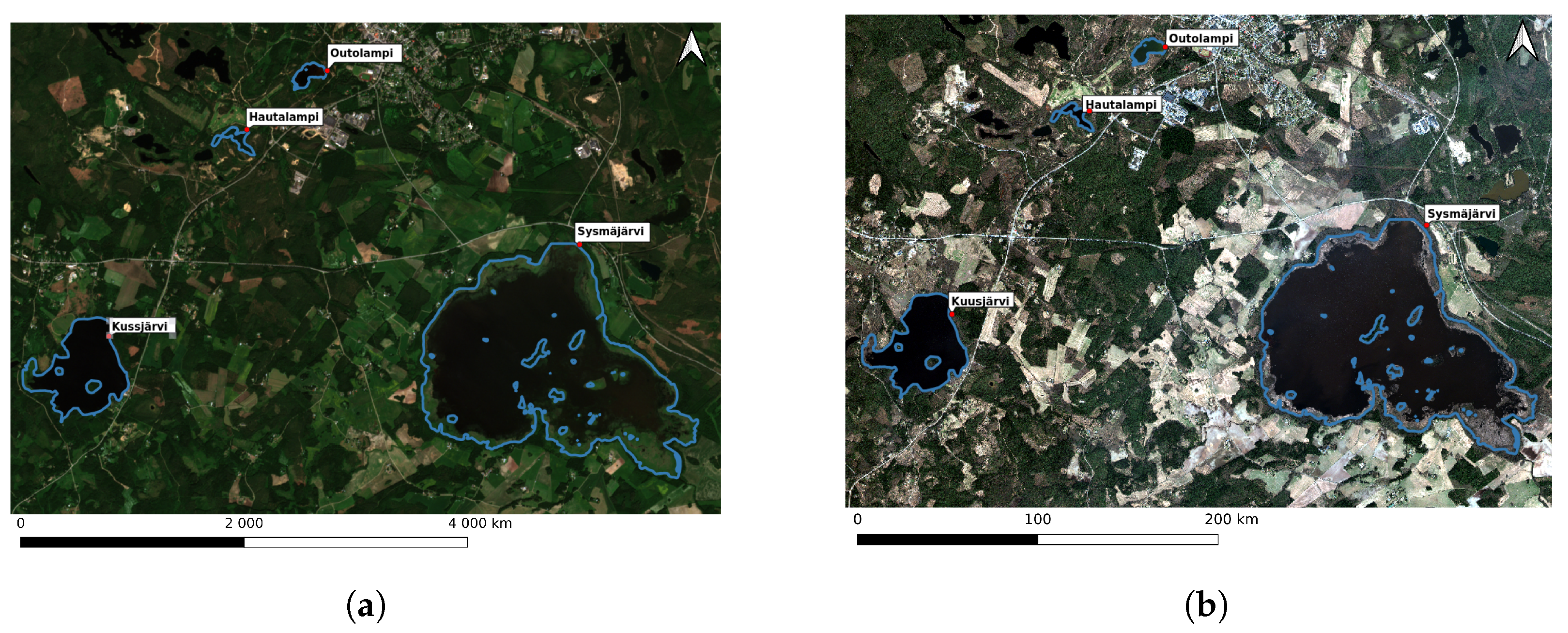
• Experiments from three AMD lakes: We conducted our experiments by evaluating ML algorithms on three AMD-affected lakes in a historical mining area in Outokumpu, Finland.

2. Research Area and Datasets

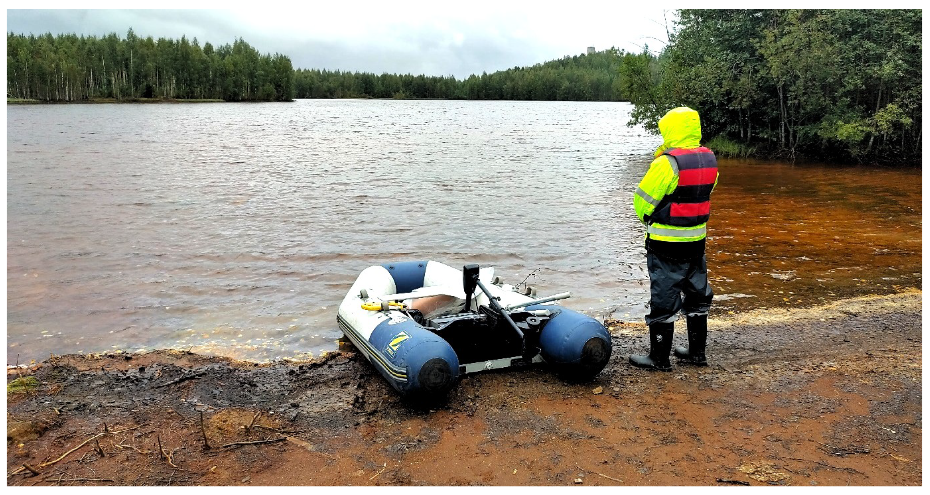
The research area includes four small humic shallow lakes in the municipality of Outokumpu located in the North Karelia region in Eastern Finland (Figure 1). In the area, mining operation began in the 1910s with the discovery of the Outokumpu volcanogenic massive sulfide (VMS) ore deposit, which later gave name to the Outokumpu-type deposits of similar geological settings [25,26]. Underground mining activities were performed from three mines called the Old mine, the Mökkivaara mine, and the Keretti mine, from which various metals, including Cu, Zn, and Co, were extracted between the years 1913 and 1989.

The mining activities had significant environmental impacts, and large areas were affected by mine waste and low-quality drainage, especially the lakes Outolampi, Alimmainen Hautalampi, and Sysmäjärvi. Outolampi is the most acidified lake, located on the tailing area of the Old mine. From the Old mine area and Outolampi, the surface water drains into the Alimmainen Hautalampi, which has been functioning as a pond for water purification (pH raised artificially). For simplicity, we will refer to Alimmainen Hautalampi as ’Hautalampi’ throughout the remainder of the paper. From Hautalampi, the surface water drains onward to Sysmäjärvi, the largest lake of the four, which has been declared as a Natura 2000 protected area. In this study, the Kuusjärvi Lake has been included as a clean reference lake, since it should not be affected by anthropogenic acidification.

Today, some of the environmental impacts have been addressed, but, for example, Outolampi remains severely polluted, and acidification is notable in groundwater and surface waters [25]. After the termination of the mining activities, parts of the historical mining sites have been turned into cultural heritage and recreational areas, while new mining projects are under development.

2.1. Water Samples

The sampling at the Outolampi, Hautalampi, Sysmäjärvi, and Kuusjärvi lakes was conducted during 20–21 May 2024 by the Geological Survey of Finland (GTK) (https://www.gtk.fi/, 20 May 2024). As shown in Figure 1, in total, 10 surface water measurements and samples were taken: two from Kuusjärvi (S1, S2), two from Outolampi (S3, S4), one from Hautalampi (S5), and five from Sysmäjärvi (S6–S10). The sampling points were selected randomly, ensuring they were neither too close to the shore nor clustered together. Additionally, we distributed the points across different areas of the lake to capture a range of acidification levels and provide a more representative sample of the AMD effects. The pH was measured with a portable multiparameter YSI probe, which was calibrated to pH values of 4 and 7 before fieldwork. The Outolampi had the lowest pH values (2.74–2.81), while the other lakes had more neutral pH values; Hautalampi had a value of 6.28, Sysmäjärvi had the range 4.39–6.55, and Kuusjärvi had the range 6.46–6.54. The sampling was conducted in Outolampi, Hautalampi, and Kuusjärvi utilizing a small rubber boat (Figure 2), and in Sysmäjärvi it was conducted with a small aluminium boat with an outboard motor. The sampling weather was sunny, with an air temperature of around 10–13 °C.

2.2. Satellite Imagery

For this study, we utilized satellite data from two sources: Sentinel-2 and Worldview-3.

Table 1. Description of input data sources used in this study.

Sensor	Band	Central Wavelength (nm)	Bandwidth (nm)	Spatial Resolution (m)
Sentinel-2	B2-Blue	490	65	10
	B3-Green	560	35	10
	B4-Red	665	30	10
	B5-Red Edge1	705	15	20
	B6-Red Edge2	740	15	20
	B7-Red Edge3	783	20	20
	B8-NIR	842	115	10
	B8A-NIR	865	20	20
	B11-SWIR1	1610	90	20
	B12-SWIR2	2190	180	20
WorldView-3	Panchromatic	470	100	0.4
	B1-Coastal	400	20	1.6
	B2-Blue	450	50	1.6
	B3-Green	510	50	1.6
	B4-Yellow	580	50	1.6
	B5-Red	660	60	1.6
	B6-Red Edge	725	40	1.6
	B7-NIR1	830	100	1.6
	B8-NIR2	950	100	1.6

provides a detailed specification of the bands used from both the Sentinel-2 and WorldView-3 satellite data, including their central wavelength, bandwidth, and spatial resolution.

2.2.1. Sentinel-2

Two applicable Sentinel-2 (S2) images were downloaded from FinHub service (https://finhub.nsdc.fmi.fi/#/home) for the period from 28 May and 17 June 2024 to quantitatively assess AMD in three study lakes near to water samples acquisition time. For AMD-related tasks, the preferred choice is typically Sentinel-2 Level-2A data due to the capacity for atmospheric correction and suitability for water quality assessment. Previous research has demonstrated that level-2A data enable more accurate detection of changes in water bodies and enhance the identification of AMD-affected areas [9].

Figure 3a shows one of the Sentinel-2 images used in the Outokumpu region in this study, highlighting four study lakes. Sentinel-2 has low-to-medium spatial resolution (4 × 10 m bands, 6 × 20 m bands, 3 × 60 m bands). Features used for modeling included pixel values from all the bands with 10–20 m initial resolutions (see Table 1), where the 20 m bands were resampled to 10 m pixel size to enable production of single-file multiband rasters. Therefore, we considered 10 bands for each Sentinel-2 datapoint of imagery with the resolution 10 m.

2.2.2. Worldview-3

WorldView-3 (WV3) is a high-resolution satellite recognized for its outstanding spatial and spectral capabilities. As shown in Table 1, we used nine bands, including eight multispectral bands (covering visible to near-infrared) and a panchromatic band for high-resolution imagery. A WV3 image from 15 May 2024 was selected, as its acquisition time is close to that of the Sentinel-2 data and water samples. The eight multispectral bands have a resolution of 1.6 m, while one panchromatic band has a resolution of 0.4 m. For consistency in analysis, all nine bands were resampled to a resolution of 1.6 m. Figure 3b shows the true-color image of the WV3 image used in this study.

2.3. Dataset Description

There are two approaches to generating the dataset: (1) training ML models on a combined dataset from all lakes or (2) training models on a separate dataset for each lake. Each approach has its own advantages and disadvantages. Based on our experiments and the water sample data (ground truth) provided in Section 2.2, we found that the second approach was more reliable for our study. This conclusion came from the variation in pH values in different lakes, reflecting different levels of acidity and alkalinity. For instance, Outolampi exhibits very low pH values (highly acidic), whereas Kuusjärvi and Sysmäjärvi have higher pH values, ranging from neutral to near-neutral values. These differences indicate that each lake has distinct characteristics in terms of pH and other critical parameters. Consequently, training separate models for each lake allows the models to more effectively capture the specific patterns and relationships within each lake’s data. While this approach initially requires field data for each lake, once trained, these models can be applied to similar lakes with minimal additional fieldwork if the lakes share similar characteristics.

In this study, we utilized the spectral bands from S2 and WV3 as features for our ML models to enhance the prediction of AMD indicators. To ensure consistency in spatial resolution, we employed the bilinear interpolation technique to upsample Sentinel-2 data to match the 1.6 m resolution of WV3. Specifically, we combined the bands from these two sources at the initial stage of data preparation. This integration at the “early fusion” level allowed us to create a comprehensive feature set that leverages the complementary strengths of S2 and WV3 data. As a result, each sample in our dataset is represented by a total of 29 features: 20 bands from two S2 images and 9 bands from WV3. We used these two S2 images primarily because they were the only available images from a similar time frame as the WV3 imagery and provided complete coverage of all the lakes. Additionally, using two S2 images allowed the model to capture temporal variation. Two labels were assigned to each sample, since we assumed two problems related to AMD mapping in this study, including the following:

• Classification (AMD detection): We tackled the classification problem of identifying AMD-affected areas using multispectral imagery from Sentinel-2 and high-resolution imagery from WorldView-3. The classification task aims to label each pixel as either AMD-affected or non-AMD-affected.
• Regression (quantitative pH mapping): The regression problem involves predicting and visualizing the pH values of water bodies using the same set of remote sensing features (bands).

We performed a binary classification where each sample was labeled either AMD (class 1) or non-AMD (class 0). We classified a lake as AMD-affected not solely based on pH levels but also on its exposure to drainage from mining activities, which may introduce contaminants. While low pH is a strong indicator, some AMD-affected lakes in our study may have relatively higher pH levels while still receiving AMD-related drainage. The clean lake sample (Kuusjärvi), having no indication of AMD contamination, was labeled as non-AMD. AMD lakes (Outolampi, Hautalampi, and Sysmäjärvi), on the other hand, were identified as those showing signs of acidification from mining activities, in addition to the natural acidity levels typical of humic lakes, as indicated by previous environmental studies. By integrating samples from AMD-affected lakes and the clean lake, we created a comprehensive dataset. The generated dataset allowed for more effective training of ML models for both classification (AMD vs. non-AMD) and regression (pH prediction). The inclusion of clean lake data provided a critical baseline for identifying non-AMD conditions, thus improving the model’s ability to differentiate between AMD and non-AMD samples. The final dataset was divided into training and testing sets in an 80:20 ratio.

3. Methods

3.1. Data Augmentation

We enhanced the robustness of the proposed ML models by proposing a data augmentation strategy due to the limited number of water samples. We generated additional samples around each known water sample location using a window size specific to each lake, as determined by geological experts. In our study, the window size was chosen based on factors such as the spatial distribution of AMD-affected areas, the need to avoid shorelines to reduce edge effects, and the observed variability in mineralization patterns across different parts of each lake. This approach was applied consistently across all lakes to ensure that the augmented samples accurately reflected the characteristics of their respective environments. In addition, we took care to avoid regions with dense vegetation or shallow waters for choosing non-AMD samples, as these factors have been shown to interfere with AMD detection [7]. The selection of non-AMD areas was based on available water sample data and expert guidance, prioritizing regions with clearer water.

Figure 4 illustrates an example of the proposed approach for Outolampi lake, which was chosen to maintain the homogeneity of the augmented samples. For example, we considered a square area with a length and width of 48 m for the Outolampi lake. Given the spatial resolution of 1.6 m, the window size is 30 × 30 pixels (48 m/1.6 m = 30). The water sample point is located in the center of the window with coordinates $(x,y)$, so the top left pixel would be at coordinates $(x-15,y-15)$. The window sizes were chosen to ensure that the selected areas accurately represented either AMD-affected or non-AMD-affected characteristics of the lake. For the classification, pixels were labeled as “class 1” and “class 0” inside the window around each water sample for an AMD lake and a clean lake, respectively. For regression, the pixels inside the windows were assigned with the same pH level, such as water samples.

Table 2. The number of AMD and non-AMD samples for each lake after data augmentation.

Lake	Total Samples	Window Size	Number of AMD Samples	Window Size of Kussjärvi	Number of Non-AMD Samples
Sysmäjärvi	38,000	96 m	18,000	160 m	20,000
Outolampi	4250	46 m	1800	56 m	2450
Hautalampi	4250	46 m	1800	56 m	2450

shows the window size for each lake and the number of samples for both AMD and non-AMD classes in the dataset after data augmentation. As you can see in Table 2, we assumed that the different window size of Kussjärvi depends on the size of the AMD lake to generate a balanced data set. For example, in Hautalampi, which is the smallest lake with fewer AMD samples, we used a smaller window size for Kuusjärvi. Conversely, for Sysmäjärvi, the largest lake with a higher number of AMD samples, we chose a larger window size for Kuusjärvi. This approach helped balance the classes distribution of AMD and non-AMD samples.

3.2. Machine Learning Methods

3.2.1. K-Nearest Neighbors

The K-Nearest Neighbors algorithm (KNNs) [23] is a widely applied ML method. KNNs can be used for both classification and regression tasks. For classification, neighbors are drawn from a set of objects with known class labels, while for regression, neighbors are drawn from a set of objects with known property values. This set of known objects constitutes the training set for the algorithm, although the KNNs does not require an explicit training phase. The KNNs has several advantages: it is non-parametric, meaning it does not require parametric models for estimation or classification. It can determine all output variables of interest simultaneously, preserving the covariance structure of the training data variables. Additionally, since the KNNs does not extrapolate values beyond the training data, it avoids unrealistic estimations when the feature space of independent test data differs from that of the training data. In our analyses, we optimized the KNNs method using the hyperparameter set $k=3,5,7,9,11,13$, selecting the value that minimized error in cross-validation. This optimization process allowed us to balance model simplicity and prediction accuracy, enhancing KNNs’ effectiveness in predicting AMD indicators.

3.2.2. Random Forest

The Random Forest (RF) algorithm [22] is a decision tree-based method that enhances prediction accuracy by using multiple decision trees. Each node in a decision tree tests an input feature, and each branch represents the result of the test. By testing various multibranched decision trees, the RF selects the one that offers the best prediction. This approach allows the RF to model complex interactions within the feature space formed by the input data, making it particularly effective in high-dimensional feature spaces. Although individual decision trees can be prone to overfitting, the RF mitigates this by combining multiple trees. This method typically requires a sufficient number of observations in the training data to be effective. The RF is commonly used in remote sensing applications where numerous input features are involved. Another advantage of the RF is its ability to assess model performance through out-of-bag (OOB) error estimation. Since each tree is trained on a different bootstrap sample, a portion of the data remains unused in each tree’s construction and can be used as a validation set to evaluate the ensemble’s performance, thus providing a reliable OOB error metric without needing separate validation data.

In our study, we employed an RF model consisting of 100 decision trees, each with a maximum depth of 100. This configuration helps balance the model’s complexity and its ability to generalize from the training data.

3.2.3. Multilayer Perceptron

Multilayer perceptron (MLP) [24] is a type of simple feedforward neural network composed of multiple layers of perceptrons. Typically, an MLP includes at least three layers: an input layer, a hidden layer, and an output layer. The primary goal of an MLP in prediction tasks is to minimize the difference between the network’s output and the target values by adjusting the weights of the inputs within its layers.

MLPs, and neural networks in general, are usually trained using gradient descent-based backpropagation algorithms. These algorithms evaluate the network’s performance on the training data, then update the network weights layer by layer by moving backwards through the network—a process known as backpropagation. Given the typically large number of weights in a neural network, it can be computationally infeasible to perform these iterative updates using the entire dataset. Consequently, especially in deep learning contexts, stochastic versions of backpropagation are used. These algorithms update the weights using random smaller samples of the training data. In this study, we used an MLP architecture with two hidden layers consisting of 64 and 32 nodes, respectively. The MLP model was trained using the backpropagation algorithm with a maximum of 50,000 iterations. To prevent overfitting, early stopping was employed, where training halts if there is no improvement in the validation error over a defined number of iterations. This configuration was selected to balance model complexity and computational cost, allowing the MLP to effectively capture the intricate relationships in our dataset while avoiding unnecessary training cycles that could lead to overfitting.

3.3. Cross-Validation

Cross-validation [27] is a widely used resampling technique in ML that aims to evaluate a model’s performance and generalization capability. One popular variant is k-fold cross-validation, where the dataset is divided into k equally sized folds. The model is trained on $k-1$ folds and evaluated on the remaining fold, with this process repeated k times. The performance measures from each iteration are averaged to estimate the model’s overall performance. The advantages of cross-validation are manifold. It provides a more reliable estimate of a model’s generalization performance compared to a single train–test split, since it evaluates the model on multiple independent data subsets. In addition to k-fold cross-validation, there is another variant called stratified cross-validation. Stratified k-fold cross-validation is a variation in which the dataset is divided into folds such that each fold has approximately the same class distribution as the original data set. This is especially useful for imbalanced datasets, ensuring that each fold is representative of the overall class distribution, leading to a more reliable assessment of the model’s performance across all classes. We used a 10-fold stratified cross-validation in our work to assess the performance of the ML algorithms.

We employed the Greedy Forward Selection (GFS) method [28] for each model to select the best hyperparameters and identify the most relevant features for the model. GFS begins with an empty set of features and iteratively adds the feature that improve the model’s performance the most based on a predefined criterion such as cross-validation accuracy. This procedure continues until adding more features does not significantly enhance the model’s performance.

4. Results

4.1. Classification Results (AMD vs. Non-AMD)

4.1.1. Performance Metrics

The models were trained using the selected features identified by GFS. We used four widely used metrics to measure the performance of ML models on the test dataset: overall accuracy, sensitivity, specificity, and F1-score. The formula used are the following:

$$Sensitivity={\displaystyle \frac{TP}{TP+FN}}$$

(1)

$$Specificity={\displaystyle \frac{TN}{TN+FP}}$$

(2)

$$Accuracy={\displaystyle \frac{TN+TP}{TN+FP+TP+FN}}$$

(3)

$$Precision={\displaystyle \frac{TP}{TP+FP}}$$

(4)

$$F1\text{-}score=2\times {\displaystyle \frac{precision\times Sensitivity}{precision+Sensitivity}}$$

(5)

where $TP$, $FP$, $TN$, and $FN$ indicate the total number of true positive, false positive, true negative, and false negative pixels, respectively.

Table 3. Comparison of MLP, KNNs, and RF models for Sysmäjärvi, Outolampi, and Hautalampi based on overall accuracy, sensitivity, specificity, and F1-score.

Metric	Model	Sysmäjärvi	Outolampi	Hautalampi
Overall Accuracy (%)	MLP	50.68	73.90	97.79
	KNNs	46.33	57.03	74.82
	RF	48.20	70.31	76.45
Sensitivity (%)	MLP	52.00	74.50	98.00
	KNNs	46.00	57.00	75.00
	RF	49.00	71.00	77.00
Specificity (%)	MLP	50.00	73.00	97.50
	KNNs	46.00	57.50	74.50
	RF	48.00	69.50	76.00
F1-Score	MLP	51.00	74.00	97.80
	KNNs	46.10	57.10	74.90
	RF	48.50	70.70	76.20

shows the performance metrics in the test data set for ML methods to classify AMD and non-AMD samples in three lakes. The results show that the MLP model consistently achieved the highest overall accuracy across all three lakes, with particularly high performance in Hautalampi (97.79%). This suggests that MLP is more capable of accurately distinguishing between AMD and non-AMD areas compared to KNNs and RF models. The RF also performed relatively well, with an accuracy of 70.31% in Outolampi. Specificity, reflecting the ability to correctly identify non-AMD areas, was also highest for the MLP model, with Hautalampi again showing the strongest performance (97.50%). The highest F1-score was recorded for Hautolampi (97.80%), which aligns with its overall strong performance metrics. Another observation from the results is the MLP accuracy was notably lower for Sysmäjärvi, with an accuracy around 50%. This reduced performance can be attributed to the similarity in pH values between Sysmäjärvi and Kuusjärvi. This result suggests that additional distinguishing features or alternative indicators may be necessary to enhance classification accuracy in environments where AMD- and non-AMD-affected areas share similar spectral or environmental characteristics.

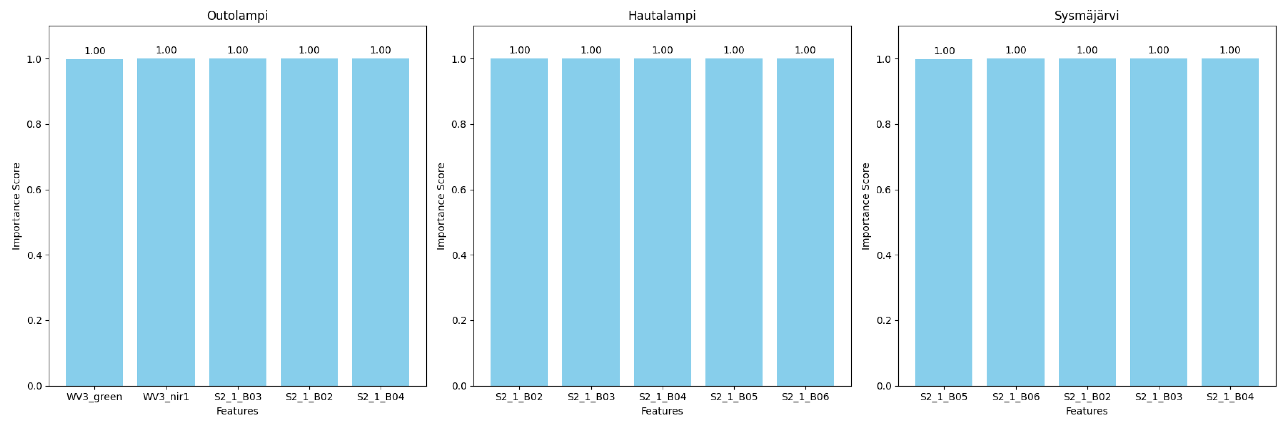
4.1.2. Feature Importance

We used the permutation-based feature importance method. This method assesses the importance of each feature by measuring the decrease in the model’s performance when the values of that feature are randomly shuffled, or “permuted”, while keeping all other features constant. Figure 5 visualizes the top-five features and their importance scores as determined by MLP as the best classifier for predicting AMD indicators across three study lakes. We present only the five most important features, as features beyond the fifth had a negligible impact on the model’s performance. The importance scores range from 0 to 1, with a score of 1.0 indicating maximum importance for the model’s predictive performance. For each lake, the selected features include bands from both WV3 and S2 imagery. From this result, we can see all five top features in all lakes have an importance score of 1.00, showing their equal and significant contribution to the model’s performance. Outolampi relies heavily on the WV3 features (green and NIR1) along with Sentinel-2 bands (B3, B2, and B4). Hautalampi and Sysmäjärvi mainly rely on the Sentinel-2 bands (B2, B3, B4, B5, and B6). This uniform importance score highlights the robustness of these specific spectral bands in capturing the unique characteristics of AMD-affected waters, regardless of location. In [6], they also showed that Sentinel B02 (490 nm) and Sentinel B08 support in the detection of metal content in AMD environments while Sentinel B4 is useful to individuate Fe. Furthermore, the differences in feature importance across lakes suggest that local environmental conditions, such as pH variations or mineral concentrations, may influence the effectiveness of different spectral bands for AMD detection. For example, bands sensitive to specific minerals may be more relevant in lakes with higher mineral contents, which could explain the variance in feature importance observed across the three lakes. Another main observation from this result is that only the bands from the first Sentinel-2 image (28 May 2024), S2_1, appear among the top features. This does not indicate that the second Sentinel-2 image was excluded. However, the permutation importance results suggest that the features from the first image were more informative for distinguishing AMD-affected areas. This difference could be due to temporal variations between the two Sentinel-2 images, where environmental conditions in the first image provided stronger predictive cues. Such temporal differences highlight the potential impact of selecting multiple image acquisitions and reinforce the importance of considering seasonal or daily changes when analyzing time-series satellite data.

4.1.3. AMD Classification Maps

The classification maps generated using the MLP model (which exhibited the highest accuracy) are shown in Figure 6 for each lake. These maps highlight the areas identified as AMD and non-AMD across the three lakes in the Outokumpu mining area. The vast majority of the lake’s area has been classified as AMD-affected instead of a small region near the shore being classified as non-AMD. Therefore, these maps show that the lakes are largely affected by AMD. In the next subsection, we can obtain more sights about the pH distribution of AMD and non-AMD area in each lake.

4.2. Regression (Quantitative pH Mapping)

4.2.1. Performance Metrics

Table 4. RMSE of regression models on the test dataset.

Lake	KNNs	MLP	RF
Sysmäjärvi	0.30	0.25	0.26
Outolampi	0.32	0.27	0.30
A. Hautalampi	0.20	0.10	0.17

presents the Root Mean Squared Error (RMSE) for three regression models on the test dataset. The results show that the MLP model outperformed both the KNNs and RF, showing the lowest RMSE, indicating that it provides the most accurate predictions. The RF model performed moderately well, with better performance than the KNNs but not as well as the MLP, as indicated by its RMSE. The KNNs model showed the least favorable performance among the three models, with the highest RMSE, indicating it has the largest prediction errors and explains the least amount of variance in the data.

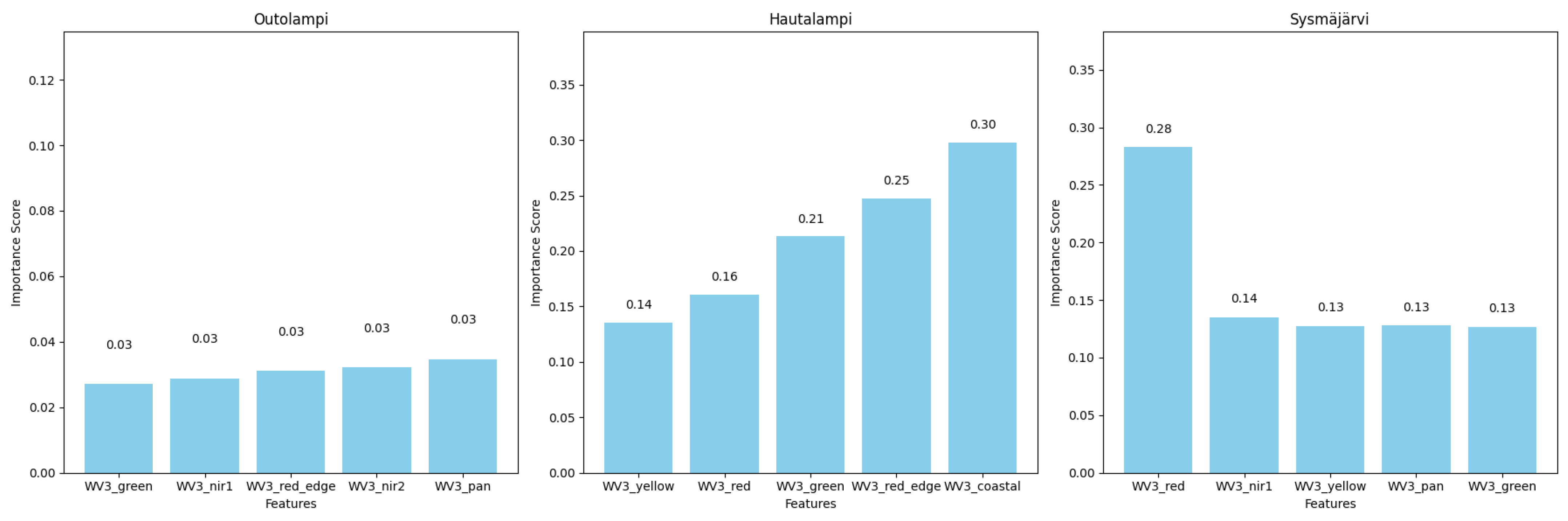
4.2.2. Feature Importance

Figure 7 illustrates the feature importance scores by the best regressor (MLP) for three lakes. In Outolampi, the model assigned nearly equal importance to five WV3 features, with each feature having a relatively low importance score of 0.03. In Hautalampi, the model showed a clear preference for specific features. The WV3 Coastal band was the most important feature, with a score of 0.30, followed by the Red Edge and Green bands. Similarly to Hautalampi, the model gave the highest importance score to the WV3 Red band, with a score of 0.28 in Sysmäjärvi. The fact is that pH by itself is not an optically detectable property. It relates to other properties of the water that can determine acidification, such as metal content. The satellite bands that provided reliable results for Sysmäjärvi and Hautalampi differ in part from those reliable for Outolampi; this might be related to the content of the water. Outolampi has 100 times higher concentration of metals compared to Sysmäjärvi and Hautalampi and very low pH values. The pH can determine the formation of different minerals starting from same metals ions and minerals have different spectrum. In [29], several bands were used to assess water quality as 490–560 nm (Sentinel B2, B3, and B4) in the determination of phytoplacton, chromophoric dissolved organic matter, and sediments in suspension. However, pH serves as an overall indicator of the lake’s environmental condition, as it reflects the combined influence of these water quality components and their interactions.

4.2.3. Residual Plot

Figure 8 illustrates the residual plot of the MLP model on the test dataset from all lakes. The red dashed line represents a perfect prediction line where the predicted values exactly match the actual values. The residual plot represents the difference between the actual and predicted values against actual values. It also can show how the prediction errors change across different pH levels (from around 2.5 to 6.5). A horizontal red line at zero represents the ideal case of no prediction error. The result shows smaller residuals near the upper end of the pH range, indicating better prediction accuracy for higher pH values. This highlights a pattern of the model performing more accurately as the pH increases. In our dataset, there appear to be distinct clusters of points at specific pH levels (around 3, 4.5, and 6.5). These clusters arise from the discrete pH values of the 10 water samples used for validation, which were collected at these specific levels. However, the predicted values generated by the model display a more continuous spread across the pH range from 2 to 7, indicating that the model attempts to capture variations across the entire spectrum beyond the discrete validation points.

4.2.4. pH Prediction Maps

Figure 9 shows the predicted pH maps of the best model (MLP) for all lakes. The visualization indicates that the MLP model accurately estimates the pH values of the water samples, as reflected in the maps. We also observe that the pH values tend to be lower near the shore compared to the center of the lake, which can be attributed to various environmental factors such as water depth, vegetation presence, and mud in shallow areas. As noted by Riaza et al. [7], these factors can alter spectral signatures and complicate AMD mapping. To mitigate these effects, we applied vegetation masking around the shorelines, which helped the model provide more accurate pH estimations across the lakes.

In addition, in Figure 9, we observe that certain areas predicted to have lower pH values by the regression model were classified as non-AMD by the classification model. This apparent contradiction may arise from differences in model objectives and feature interpretation. The classification model, being binary, likely identifies broad patterns or thresholds to separate AMD and non-AMD areas, potentially missing finer pH variations within each class. Conversely, the regression model estimates pH on a continuous scale, capturing subtle gradients in acidity that might not be distinct enough to trigger a classification as AMD-affected. This discrepancy highlights the complementary nature of classification and regression models, suggesting that combining both approaches may improve the robustness of AMD mapping.

4.3. Multi-Modal vs. Uni-Modal

To demonstrate the ability of fusing two data sources, Sentinel-2 and WorldView-3 (WV3), we evaluated the MLP model using each input source individually, as well as in combination for both classification and regression tasks across different lakes.

Table 5. Performance comparison between unimodal MLP and multimodal MLP frameworks.

Task	Lake	Input Source	Accuracy (Classification) %	RMSE (Regression)
Classification	Sysmäjärvi	S2	45.10	-
		WV3	45.69	-
		S2 + WV3	50.68	-
	Outolampi	S2	53.80	-
		WV3	58.39	-
		S2 + WV3	73.90	-
	Hautalampi	Sentinel-2	73.05	-
		WV3	75.78	-
		S2 + WV3	97.79	-
Regression	Sysmäjärvi	S2	-	0.36
		WV3	-	0.29
		S2 + WV3	-	0.25
	Outolampi	S2	-	0.35
		WV3	-	0.32
		S2 + WV3	-	0.27
	Hautalampi	S2	-	0.21
		WV3	-	0.18
		S2 + WV3	-	0.10

compares the performance of unimodal (single-source) and multimodal (dual-source) frameworks. From the results, we observe two main findings:

• The multimodal framework (Sentinel-2+WV3) consistently outperformed the unimodal frameworks across all lakes for both regression and classification tasks. The MLP classifier achieved the highest accuracy (97.79%) when both data sources were combined. For regression tasks, the multimodal framework also demonstrated superior performance, particularly for Hautalampi, with an RMSE of 0.10.
• The framework based on WV3 data alone outperformed the Sentinel-2-based framework for all lakes, highlighting the value of WV3’s higher spatial resolution in improving model performance.

The integration of Sentinel-2 and WorldView-3 data significantly enhances the performance of ML models for both AMD classification and pH prediction. The combined use of multispectral and high-resolution imagery provides more robust and accurate assessments, demonstrating the effectiveness of a multimodal framework in environmental monitoring and water quality assessment.

5. Conclusions

This study advances the application of machine learning in remote sensing for environmental monitoring, specifically in the context of Acid Mine Drainage (AMD) detection and water quality assessment, showcasing the benefits of combining multispectral and high-resolution imagery. By applying Random Forest, K-Nearest Neighbors, and Multilayer Perceptron models to both classification and regression tasks, we demonstrated that this combined approach offers superior performance in distinguishing AMD-affected areas and predicting pH levels compared to using individual datasets. The experimental results were collected on three lakes in the Outokumpu mining region, Finland. The results show that the MLP model achieved the highest classification accuracy at 97.79%, while the MLP regressor achieved a root mean square error of 0.10 for pH estimation, underscoring its effectiveness in this application.

In future works, we plan to explore alternative feature selection methods to refine our understanding of feature importance beyond the current permutation-based approach. Additionally, we aim to validate that the top features reflect relevant AMD indicators, such as iron or sulfate absorption, rather than potential overfitting. Lastly, we will investigate how local environmental factors, like pH and mineral concentrations, influence spectral band effectiveness, enhancing model accuracy for AMD detection across diverse lake conditions.

References

1. Singer, P.; Stumm, W. Acidic mine drainage: The rate-determining step. Science 1970, 167, 1121–1123. [Google Scholar] [CrossRef] [PubMed]
2. Ong, C.C.H.; Cudahy, T.J. Mapping Contaminated Soils: Using Remotely-Sensed Hyperspectral Data to Predict pH. Eur. J. Soil Sci. 2014, 65, 897–906. [Google Scholar] [CrossRef]
3. Williams, D.J.; Bigham, J.M.; Cravotta, C.A., III; Traina, S.J.; Anderson, J.E.; Lyon, J.G. Assessing mine drainage pH from the color and spectral reflectance of chemical precipitates. Appl. Geochem. 2002, 17, 1273–1286. [Google Scholar] [CrossRef]
4. Frau, F.; Medas, D.; Da Pelo, S.; Wanty, R.; Cidu, R. Environmental Effects on the Aquatic System and Metal Discharge to the Mediterranean Sea from a Near-Neutral Zinc-Ferrous Sulfate Mine Drainage. Water Air Soil Pollut. 2015, 226, 55. [Google Scholar] [CrossRef]
5. Sánchez-España, J. Acid Mine Drainage in the Iberian Pyrite Belt: An Overview with Special Emphasis on Generation Mechanisms, Aqueous Composition and Associated Mineral Phases. Macla 2008, 10, 34–43. [Google Scholar]
6. Seifi, A.; Hosseinjanizadeh, M.; Ranjbar, H.; Honarmand, M. Identification of Acid Mine Drainage Potential Using Sentinel 2a Imagery and Field Data. Mine Water Environ. 2019, 38, 707–717. [Google Scholar] [CrossRef]
7. Riaza, A.; Buzzi, J.; García-Meléndez, E.; Carrère, V.; Sarmiento, A.; Müller, A. Monitoring acidic water in a polluted river with hyperspectral remote sensing (HyMap). Hydrol. Sci. J. 2015, 60, 1064–1077. [Google Scholar] [CrossRef]
8. Isgro, M.; Basallote, M.; Caballero, I.; Barbero, L. Comparison of UAS and Sentinel-2 Multispectral Imagery for Water Quality Monitoring: A Case Study for Acid Mine Drainage Affected Areas (SW Spain). Remote Sens. 2022, 14, 4053. [Google Scholar] [CrossRef]
9. Hanelli, D.; Barth, A.; Volkmer, G.; Köhler, M. Modelling of Acid Mine Drainage in Open Pit Lakes Using Sentinel-2 Time-Series: A Case Study from Lusatia, Germany. Minerals 2023, 13, 271. [Google Scholar] [CrossRef]
10. Kopačková, V. Mapping Acid Mine Drainage (AMD) and Acid Sulfate Soils Using Sentinel-2 Data. In Proceedings of the IGARSS 2019—2019 IEEE International Geoscience and Remote Sensing Symposium, Yokohama, Japan, 28 July–2 August 2019; pp. 5682–5685. [Google Scholar] [CrossRef]
11. Rendana, M.; Idris, W.; Abd Rahim, S. Mapping Chini Lake (Pahang, Malaysia) using Sentinel-2 images to determine the effect of acid mine drainage in the pre- to post-COVID-19 restriction period. Environ. Monit. Assess. 2022, 195, 205. [Google Scholar] [CrossRef] [PubMed]
12. Farahnakian, F.; Heikkonen, J. Deep Learning Based Multi-Modal Fusion Architectures for Maritime Vessel Detection. Remote Sens. 2020, 12, 2509. [Google Scholar] [CrossRef]
13. Sanliyuksel Yucel, D.; Yucel, M.; Baba, A. Change detection and visualization of acid mine lakes using time series satellite image data in geographic information systems (GIS): Can (Canakkale) County, NW Turkey. Environ. Earth Sci. 2014, 72, 4311–4323. [Google Scholar] [CrossRef]
14. Pascucci, S.; Pignatti, S.; Belviso, C.; Cavalcante, F.; Bogliolo, M. Worldview-3 and Sentinel-2 Imagery for Mapping Naturally Occurring Asbestos (NOA) in Serpentinites Rocks in Southern Italy. In Proceedings of the IGARSS 2019—2019 IEEE International Geoscience and Remote Sensing Symposium, Yokohama, Japan, 28 July–2 August 2019; pp. 6756–6759. [Google Scholar] [CrossRef]
15. Honglyun, P.; Kim, N.; Park, S.; Choi, J. Sharpening of Worldview-3 Satellite Images by Generating Optimal High-Spatial-Resolution Images. Appl. Sci. 2020, 10, 7313. [Google Scholar] [CrossRef]
16. Farahnakian, F.; Zelioli, L.; Middleton, M.; Seppä, I.; Pitkänen, T.; Heikkonen, J. CNN-based Boreal Peatland Fertility Classification from Sentinel-1 and Sentinel-2 Imagery. In Proceedings of the 2023 IEEE International Symposium on Robotic and Sensors Environments (ROSE), Tokyo, Japan, 6–7 November 2023; pp. 1–7. [Google Scholar] [CrossRef]
17. Farahnakian, F.; Zelioli, L.; Pitkänen, T.; Pohjankukka, J.; Middleton, M.; Tuominen, S.; Nevalainen, P.; Heikkonen, J. Multistream Convolutional Neural Network Fusion for Pixel-wise Classification of Peatland. In Proceedings of the 2023 26th International Conference on Information Fusion (FUSION), Charleston, SC, USA, 27–30 June 2023; pp. 1–8. [Google Scholar] [CrossRef]
18. Farahnakian, F.; Torppa, J.; Luodes, N.; Panttila, H.; Karlsson, T. A Comparative Study of Machine Learning Models for Pixel-Wise Acid Mine Drainage Classification Using Sentinel-2. In Proceedings of the IGARSS 2024—2024 IEEE International Geoscience and Remote Sensing Symposium, Athens, Greece, 7–12 July 2024; pp. 2127–2131. [Google Scholar] [CrossRef]
19. Nogueira, P.; Silva, M.; Roseiro, J.; Potes, M.; Rodrigues, G. Mapping the Mine: Combining Portable X-ray Fluorescence, Spectroradiometry, UAV, and Sentinel-2 Images to Identify Contaminated Soils—Application to the Mostardeira Mine (Portugal). Remote Sens. 2023, 15, 5295. [Google Scholar] [CrossRef]
20. Flores, H.; Lorenz, S.; Jackisch, R.; Tusa, L.; Contreras, I.C.; Zimmermann, R.; Gloaguen, R. UAS-Based Hyperspectral Environmental Monitoring of Acid Mine Drainage Affected Waters. Minerals 2021, 11, 182. [Google Scholar] [CrossRef]
21. Teru, K.K. On Data Augmentation and Consistency-based Semi-supervised Relation Extraction. In Proceedings of the First Workshop on Interpolation Regularizers and Beyond at NeurIPS 2022, New Orleans, LA, USA, 29 July–6 October 2022. [Google Scholar]
22. Breiman, L. Random Forests. Mach. Learn. 2001, 45, 5–32. [Google Scholar] [CrossRef]
23. Cover, T.; Hart, P. Nearest neighbor pattern classification. IEEE Trans. Inf. Theory 1967, 13, 21–27. [Google Scholar] [CrossRef]
24. Bishop, C. Neural Networks for Pattern Recognition; Oxford University Press: New York, NY, USA, 1995. [Google Scholar]
25. Tornivaara, A.; Turunen, K.; Lahtinen, T.; Heino, N.; Pasanen, A.; Reinikainen, J.; Jouttijärvi, T.; Häkkinen, J.; Karjalainen, N.; Viitasalo, M. Suljettujen ja hylättyjen kaivannaisjätealueiden kunnostustarpeen arviointi. 06 2020. Available online: https://julkaisut.valtioneuvosto.fi/handle/10024/162348 (accessed on 12 August 2024).
26. Geological Survey of Finland. Old Mining Waste Areas Present a Persistent Environmental Hazard: How Can Research Help to Remediate Them and Assess Their Risks? Geological Survey of Finland: Espoo, Finland, 2024. [Google Scholar]
27. Arlot, S.; Celisse, A. A survey of cross-validation procedures for model selection. Stat. Surv. 2010, 4, 40–79. [Google Scholar] [CrossRef]
28. Drobnič, F.; Kos, A.; Pustišek, M. On the Interpretability of Machine Learning Models and Experimental Feature Selection in Case of Multicollinear Data. Electronics 2020, 9, 761. [Google Scholar] [CrossRef]
29. Pisanti, A.; Magrì, S.; Ferrando, I.; Federici, B. Sea water turbidity analysis from Sentinel-2 images: Atmospheric CORRECTION AND BANDS CORRELATION. Int. Arch. Photogramm. Remote Sens. Spat. Inf. Sci. 2022, 48, 371–378. [Google Scholar] [CrossRef]
Figure 1. Geographic location of the study area in Finland (a,b) and the water sampling locations (red dots) from the lakes Kuusjärvi (c), Alimmainen Hautalampi and Outolampi (d), and Sysmäjärvi (e). The blue dashed lines present the simplified water drainage path from the Outolampi lake to the Sysmäjärvi lake. Background maps copyright National Land Survey of Finland.
Remotesensing 16 04680 g001
Figure 2. The Outolampi lake and the rubber boat that was utilized in sampling.
Remotesensing 16 04680 g002
Figure 3. True-color image of an example of (a) Sentinel-2 in 17 June 2024 and (b) Worldview-3 in 15 May 2024 over the Outokumpu region for three proposed AMD lakes (Outolampi, Hautalampi, and Sysmäjärvi) and one proposed clean lake (Kuusjärvi).
Remotesensing 16 04680 g003
Figure 4. An example of the proposed window Sizes for sample augmentation in Outolampi lake around each water sample red point which is centered at (x,y).
Remotesensing 16 04680 g004
Figure 5. Five top features and their scores of MLP classifier for Outolampi, Hautalampi, and Sysmäjärvi.
Remotesensing 16 04680 g005
Figure 6. AMD classification maps from the best model (MLP) for (a) Outolampi, (b) Hautalampi, and (c) Sysmäjärvi.
Remotesensing 16 04680 g006
Figure 7. Five top features and their scores of MLP regressor for Outolampi, Hautalampi, and Sysmäjärvi.
Remotesensing 16 04680 g007
Figure 8. The residual plot for MLP model on the test dataset from three lakes Outolampi, Hautalampi, and Sysmäjärvi.
Remotesensing 16 04680 g008
Figure 9. Distribution map of pH values from the best model (MLP) for (a) Outolampi, (b) Hautalampi, and (c) Sysmäjärvi. The predicted pH values for water samples are displayed on the images.
Remotesensing 16 04680 g009