Atmospheric Modulation Transfer Function Calculation and Error Evaluation for the Panchromatic Band of the Gaofen-2 Satellite

Abstract

In the optical satellite on-orbit imaging quality estimation system, the calculation of Modulation Transfer Function (MTF) is not fully standardized, and the influence of atmosphere is often simplified, making it difficult to obtain completely consistent on-orbit MTF measurements and comparisons. This study investigates the effects of various factors—such as edge angle, edge detection methods, oversampling rate, and interpolation techniques—on the accuracy of MTF calculations in the commonly used slanted-edge method for on-orbit MTF assessment, informed by simulation experiments. A relatively optimal MTF calculation process is proposed, which employs the Gaussian fitting method for edge detection, the adaptive oversampling rate, and the Lanczos (a = 3) interpolation method, minimizing the absolute deviation in the MTF results. A method to quantitatively analyze the atmospheric scattering and absorption MTF is proposed that employs a radiative transfer model. Based on the edge images of GF-2 satellite, images with various atmospheric conditions and imaging parameters are simulated, and their atmospheric scattering and absorption MTF is obtained through comparing the MTFs of the ground and top atmosphere radiance. The findings reveal that aerosol optical depth (AOD), viewing zenith angle (VZA), and altitude (ALT) are the primary factors influencing the accuracy of GF-2 satellite on-orbit MTF measurements in complex scenarios. The on-orbit MTF decreases with the increase in AOD and VZA and increases with the increase in ALT. Furthermore, a collaborative analysis of the main influencing factors of atmospheric scattering and absorption MTF indicates that, taking the PAN band of the GF-2 satellite as an example, the atmospheric MTF values are consistently below 0.7905. Among these, 90% of the data are less than 0.7520, with corresponding AOD conditions ranging from 0 to 0.08, a VZA ranging from 0 to 50°, and an ALT ranging from 0 to 5 km. The results can provide directional guidance for the selection of meteorological conditions, satellite attitude, and geographical location during satellite on-orbit testing, thereby enhancing the ability to accurately measure satellite MTF.

1. Introduction

The Modulation Transfer Function (MTF) is one of the most crucial characteristics of optical payloads, describing the sensor’s ability to resolve incident optical information and form spatial details in images [1]. However, the signal captured by optical satellite imaging does not solely depend on the performance of the sensor itself but is also influenced by other components of the imaging chain, particularly atmospheric radiation.

The methods used to obtain imaging sensor system MTF on-orbit measurements are primarily categorized into the slanted-edge method, the point source method, the pulse method, and the bar-pattern method. The slanted-edge method has been widely used in many satellite sensors, such as SPOT-5 [2,3], CBERS [4], CBERS-02 [5], IKONOS [6,7], QuickBird [8], ORBVIEW [9], ALOS PRISM [10], KOMPSAT [11], THEOS [12], Eros-B [13], and AlSAT-2A [14], due to its relatively modest requirements regarding both the light source and the target. Many studies have extended and analyzed the key steps in the slanted-edge method, such as adding corresponding correction steps to the calculation of Edge Spread Function (ESF) and Line Spread Function (LSF), which has improved the accuracy of the results [15,16,17,18]. However, due to incomplete standardization, differences in computational details when using the slanted-edge method can lead to significant deviations in the MTF calculation results. In response to this issue, the Committee for Earth Observation Satellites (CEOS) organized a comparative experiment of professional teams from various countries using MTF measurements in their research; none of the participants were always able to obtain the best estimate [19]. Therefore, it is very important to fully understand the calculation process and the calculation errors in the slanted-edge method to ensure that accurate and reproducible results are obtained.

The atmosphere, serving as the medium for optical signal transmission, affects the transmission of light in both the downward and upward paths, thereby directly impacting the quality of imaging and the accuracy of MTF measurements. Due to the blurring of high-frequency details in satellite images caused by the atmosphere, it is often regarded as a low-pass filter in the frequency domain. Numerous experts have described these phenomena through experimental statistics and approximate models [20,21,22,23,24,25]. Currently, the study of atmospheric effects on image quality is primarily divided into the MTF model for atmospheric absorption and scattering and the MTF model for atmospheric turbulence. Most models of atmospheric scattering and absorption MTF are based on the Small-Angle Approximation (SAA) theory and single-scattering approximation and are independent of sensor imaging systems. However, different studies show that the statistical results of experiments often depend on the instrument used and the assumptions made about the experiment or prediction [26]. Instrument parameters such as field of view, dynamic range, spatial frequency bandwidth, etc., limit the scattering angle size of the received imaging signal, thereby affecting the extent of blur in the image [27]. As is known, with an increase in atmospheric optical thickness, the multiple scattering effect of the atmosphere will be enhanced, and the coupling effect between the land and the atmosphere will also be strengthened. Therefore, an analysis of atmospheric absorption scattering MTF not only needs to consider the sensor parameters and atmospheric parameters, but also the influence of target characteristics and observation scenes. Targeted research is needed on the impact characteristics of the atmosphere on high-resolution imaging systems.

To address the aforementioned issues, this paper proposes a method for the quantitative analysis of atmospheric scattering and absorption MTF through radiative transfer model. Based on the parameters of satellite sensors, atmospheric conditions, and imaging scenario parameters, radiance images of the ground and the top of the atmosphere are simulated using actual satellite data. Then, by quantitatively comparing the changes in MTF between the ground and the top of the atmosphere, the atmospheric scattering and absorption MTF is obtained. During the analysis, a highly robust on-orbit MTF measurement process for satellite is also proposed. Based on the traditional edge measurement MTF method, through refining and improving the key steps in this method, an optimal calculation process that minimizes MTF error is achieved.

The rest of the paper is organized as follows. In Section 2 of this paper, the research area and the selected data set are briefly described. The principles and calculation processes of the satellite imaging system MTF and the atmospheric scattering and absorption MTF are presented in Section 3. In Section 4, the process accuracy of the slanted-edge method is quantitatively evaluated, and the impact of atmospheric characteristics and observation scenes on the MTF of images in different bands is calculated. Finally, an analysis and discussion are presented, and the factors that should be considered to reduce the influence of atmospheric MTF and their range of values are provided.

2. Study Area and Datasets

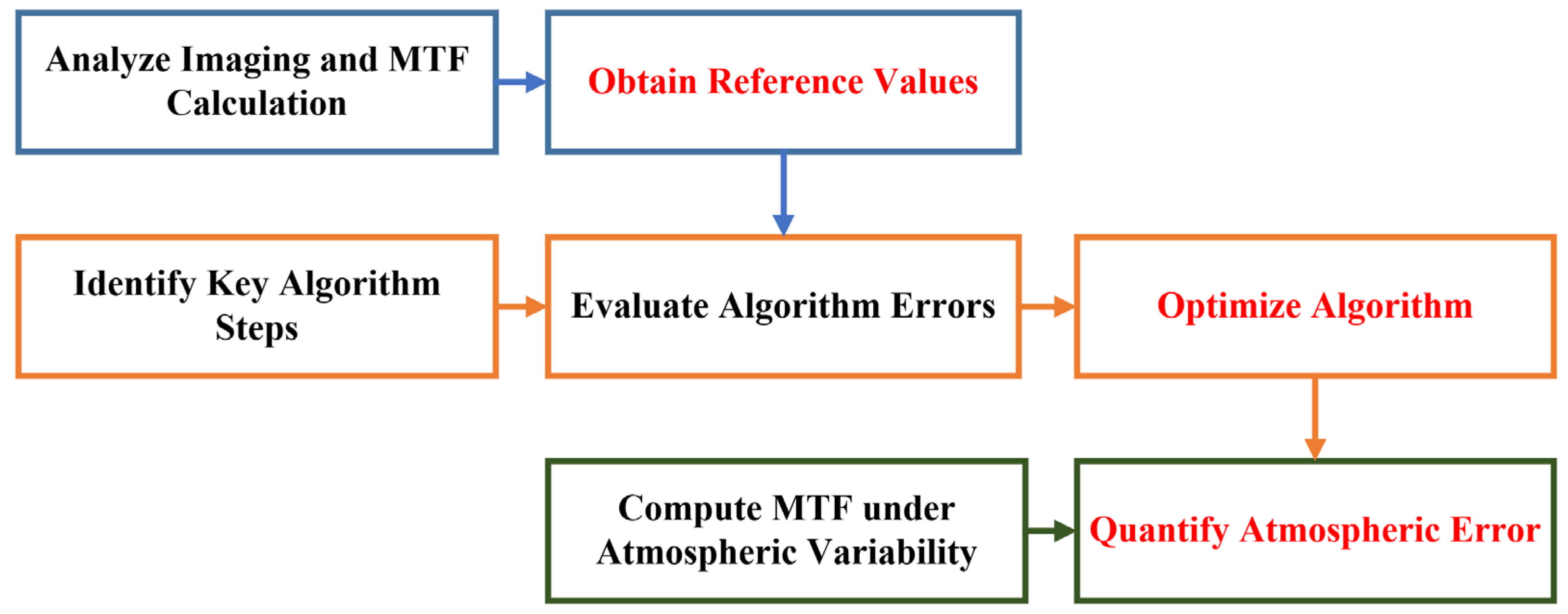
The Baotou calibration and validation site (hereinafter referred to as the “Baotou site”) located in the Inner Mongolia Autonomous Region, China, is one of the demonstration sites of the Radiometric Calibration Network (RadCalNet), providing operational radiometric calibration and validation services for high-spatial-resolution remote sensing satellite [28]. The multi-greyscale permanent artificial target in Baotou site consists of four 48 m × 48 m uniform areas, paved with natural gravel with a reflectance of approximately 8%, 20%, and 60%, respectively. In addition, there is an AERONET ground-based observation site at the Baotou site (located at 40.85°N, 109.62°E) [28,29]. AERONET is a ground-based aerosol remote sensing observation network jointly established by NASA and LOA-PHOTONS (CNRS), which can cover major regions worldwide and commercially provide atmospheric and meteorological parameters. It is also often used to verify the accuracy of satellite observations of atmospheric parameters [30].

GF-2 remote sensing satellite is a Chinese high-resolution optical satellite, which can acquire 0.8 m panchromatic (PAN) and 3.2 m multispectral (MS) images using two PMS sensors. The size of the edge target at the Baotou site can meet the MTF measurement requirements of GF-2 satellite PAN images and barely meets the requirements of MSS images [31]. According to the principle that the time-averaged atmospheric data measured by ground-based instruments can, to some extent, represent the spatial averaged atmospheric data observed by satellites [30], ground-based observations of AERONET within ±30 min of the satellite transit time over the Baotou site were selected, and the average values were used as atmospheric parameters for the satellite image. Figure 1 shows the selected GF-2 satellite image at the Baotou site on 24 October 2021 (data sourced from https://data.cresda.cn), with imaging parameters and corresponding ground-based atmospheric data (data sourced from https://aeronet.gsfc.nasa.gov), as shown in

Table 1. The GF-2 satellite imaging parameters and ground-based atmospheric data at the Baotou site on 24 October 2021.

Data Sources	Parameters	Value
GF-2 satellite parameters	Solar zenith angle/SZA (°)	54.25
	Solar azimuth angle (°)	163.12
	Viewing zenith angle/VZA (°)	2.37
	Viewing azimuth angle (°)	288.13
	Imaging time (UTC)	03:29:41
AERONET ground-based observation	Aerosol optical depth/AOD	0.1943
	Column water vapor/CWV (g/cm2)	0.4071
	Ozone/O3 (atm-cm)	0.3003
	Altitude of target/ALT (km)	1.314

.

3. Algorithm

Atmospheric scattering and absorption MTF cannot be measured directly and there is no completely standard method for calculating this. In order to investigate the influence of atmospheric scattering and absorption on the measurement of high-resolution optical satellites on-orbit MTF, the MTFs of satellite images with different atmospheric conditions were compared with the MTFs of atmospheric corrected images to achieve the estimation and analysis of atmospheric MTF. Firstly, based on the sensor parameters of the GF-2 satellite and the principle of the optical imaging system, the theoretical MTF of the GF-2 satellite at Nyquist frequency was obtained. Secondly, taking the theoretical MTF as a reference, the impact of different error terms in key steps of the slanted-edge method on the MTF results was analyzed and evaluated. In this way, the optimal robust MTF calculation process was determined. Finally, satellite images with different atmospheric conditions were simulated using a radiative transfer model based on the atmospheric corrected satellite image, and the MTFs of different images were calculated using the optimal MTF calculation process to further estimate the influence of atmospheric scattering and absorption MTF. The specific flow is shown in Figure 2.

The ISO 12233 standard specifies the conventional edge-based method used for MTF measurements [32]. When applied to the on-orbit MTF measurement of the satellite sensor, the edge target with a small angle to the detector row or column direction was selected in the remote sensing image; then, a step-edge model of the target was established, and the frequency response performance of the detector was finally evaluated using derivative calculations and Fourier calculation. The calculation of MTF in this paper was made using the slanted-edge method process suggested in the ISO 12233 standard. The main steps include selecting an edge image, detecting and fitting the edge position, constructing ESF, extracting LSF, LSF trimming, discrete Fourier transform (DFT), and normalization [15,19,32]. After performing all steps, the MTF over a range of spatial frequencies can be estimated. In the following sections, the calculation of the theoretical MTF of the satellite sensor and the method used to calculate atmospheric scattering and absorption MTF are introduced.

3.1. Estimation of Satellite Imaging System MTF

According to the linear system theory, the MTF of each part of the spaceborne optical remote sensor imaging chain can be cascaded; that is, in the frequency domain, the overall system’s MTF can be calculated by multiplying the atmospheric ${MTF}_{amt}\left(v\right)$, the optical lens ${MTF}_{opt}\left(v\right)$, the detector ${MTF}_{det}\left(v\right)$, and the electronic system ${MTF}_{amp}\left(v\right)$ [33]:

$${\mathit{MTF}}_{\mathit{sys}} \left(v\right)={MTF}_{amt}\left(v\right)·{MTF}_{opt}\left(v\right)\cdot {MTF}_{det}\left(v\right)\cdot {MTF}_{amp}\left(v\right)$$

(1)

When estimating the theoretical MTF of the satellite imaging system as a reference value for subsequent analysis, the effect of the atmospheric MTF is assumed to be an ideal value, i.e., ${MTF}_{amt}\left(v\right)=1$.

Optical lens MTF is mainly affected by diffraction and aberration [34]. Therefore, the MTF of an incoherent diffraction-limited optical system with a circular aperture can be expressed as follows:

$$\begin{array}{c}{MTF}_{opt}\left(v\right)=OTF \left(v\right)\cdot ATF \left(v\right)\\ =\left\{{\displaystyle \frac{2}{\pi }}\left[\mathrm{a}\mathrm{r}\mathrm{c}\mathrm{c}\mathrm{o}\mathrm{s} \left(v_n\right)-v_n\sqrt{1-{\left(v_n\right)}^2}\right]\right\}\cdot \left\{1-{\left({\displaystyle \frac{WF{E}_{rms}}{0.18}}\right)}^2\left[1-4{\left(v_n-{\displaystyle \frac{1}{2}}\right)}^2\right]\right\}\end{array}$$

(2)

where $v_n={\displaystyle \frac{v}{v_c}}$; $v_c={\displaystyle \frac{1}{\lambda \left(f\#\right)}}$; $v$ is the radial spatial frequency; $v_c$ is the spatial cutoff frequency; $\lambda$ is the average wavelength of each channel; $f\#={\displaystyle \frac{f}{D}}$, where $f$ is the focal length of the optical system and $D$ is the aperture of the optical system; $WF{E}_{rms}$ is the root mean square (RMS) wavefront error (WFE) in wavelengths. The RMS wavefront error value of some typical aerospace TDICCD cameras was approximately 0.13λ [35].

The sampled sensor signal was a rectangular pulse with a certain width, rather than an ideal impulse function; therefore, for a sensor with a detector pitch $p$, the sampling MTF is expressed as follows [36]:

$${MTF}_{det}\left(v\right)=\mathrm{s}\mathrm{i}\mathrm{n}\mathrm{c} \left(pv\right)$$

(3)

where $p$ is the size of the detector bin.

The passband of the imaging circuit is usually set to be wide, so the MTF degradation caused by the electronic circuit can usually be ignored, i.e., ${MTF}_{amp}\left(v\right)=1$.

The theoretical satellite imaging system ${\mathit{MTF}}_{\mathit{sys}}\left(v\right)$ can be computed using Equations (1)–(3). The point spread function (PSF) can be obtained by performing the inverse Fourier transform on ${\mathit{MTF}}_{\mathit{sys}}\left(v\right)$. By further integrating the PSF and rotating the coordinate, the ESF can be calculated:

$$ESF\left(r\right)={\int }_{-\infty }^r{\mathcal{F}}^{-1}\left\{{\mathit{MTF}}_{\mathit{sys}}\left(v\right)\right\}dt$$

(4)

where $r=x\cdot \mathit{cos}\left(\theta \right)+y\cdot \mathit{sin}\left(\theta \right)$; $\theta$ is the slant angle of the edge.

Finally, by projecting $ESF\left(r\right)$ into a two-dimensional space, the ideal edge image can be simulated using the theoretical MTF of the satellite imaging system for subsequent analysis.

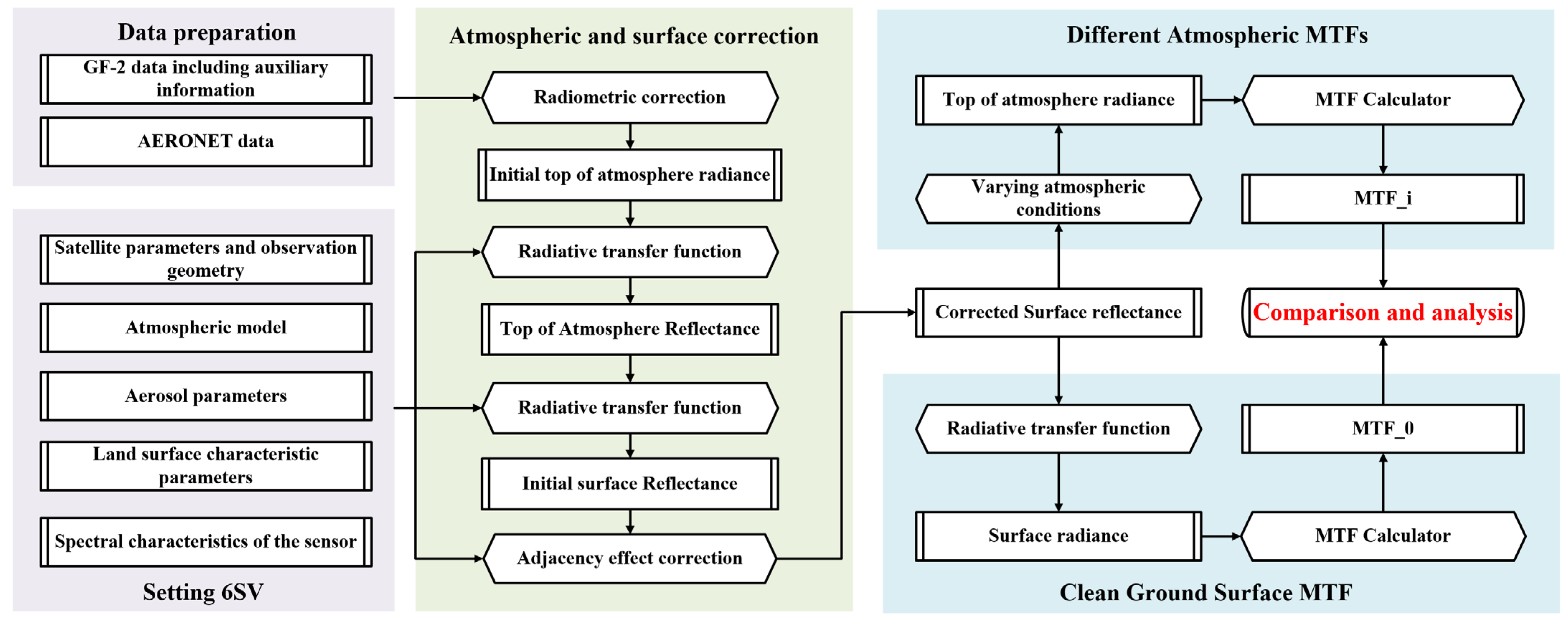
3.2. Estimation of Atmospheric Scattering and Absorption MTF

The atmospheric blurring effect on sensor imaging varies with atmospheric conditions. The MTF estimated from the radiance of satellite image reflects the comprehensive effect of the atmosphere and the sensor during imaging. The existing research based on statistical data suggests that, for on-orbit satellite optical sensors, the degradation factor of aerosol absorption and scattering at the Nyquist frequency is about 0.85 and the degradation factor of atmospheric turbulence is about 0.95, so the total atmospheric degradation factor is about 0.8 [37]. However, it is not accurate to use the constant to characterize the degradation effects of the atmosphere on image quality, and the source of error in actual on-orbit test scenarios cannot be effectively determined.

To quantitatively calculate the impact of atmosphere on the on-orbit MTF of high-resolution optical imaging satellite, the atmosphere is regarded as a whole system, with ground radiation as the input signal and top-of-atmosphere (TOA) radiation as the output signal. Images of different atmospheric conditions are simulated using a radiative transfer model. The radiative transfer model used here is the Second Simulation of a Satellite Signal in the Solar Spectrum, Vector (6SV), an advanced RT code specifically designed to simulate the reflection of radiation by a coupled atmosphere–surface system. Its simulations are in fairly good agreement with those of Monte Carlo [38]. When used for simulations of satellite observations, the input parameters of the 6SV model include solar-view geometry, atmospheric model, aerosol model, aerosol optical depth, target elevation, spectral band and spectral response function, and anisotropic and Lambertian ground conditions. By comparing the MTF of simulated ground radiation and TOA radiation, i.e., the input signal and the output signal, the atmospheric scattering and absorption MTF can be obtained. The specific process is shown in Figure 3.

Firstly, the selected GF-2 satellite image is corrected based on the calibration coefficients to obtain the top of atmosphere radiance $L_{TOA}$. Then, the imaging geometry parameters and ground-based atmospheric parameters are set as the input and the atmospheric correction is performed using the 6SV model to obtain the initial surface reflectance [39]. Permanent targets are usually paved with natural or artificial materials with uniform particles but different greyscales, so the target area is assumed to be a non-uniform Lambertian surface. For high-spatial-resolution (<100 m) imagery, the cross-radiation effects between the adjacent pixels of a non-uniform surface, also known as the adjacency effect, cannot be ignored, especially if the scene contains large reflectance contrasts [40]. Therefore, a more accurate surface reflectance ${\rho }_s$ is obtained by further correcting the influence of adjacency effects:

$${\rho }_s={\displaystyle \frac{\left(\frac{{\rho }_{TOA}}{T_g}-{\rho }_a\right)\frac{(1-⟨\rho ⟩S)}{T_s}-t_d\left({\theta }_v\right)⟨\rho ⟩}{e^{-\tau /{\mu }_v}}}$$

(5)

where ${\rho }_{TOA}$, defined as ${\rho }_{TOA}=\pi L_{TOA}/E_s{\mu }_{\mathrm{s}}$, is the top of the atmosphere reflectance; $E_s$ is the solar flux at the top of the atmosphere; ${\mu }_{\mathrm{s}}=\mathrm{c}\mathrm{o}\mathrm{s} \left({\theta }_{\mathrm{s}}\right)$ is the cosine of the SZA; $T_g$ is the gaseous transmission; ${\rho }_a$ is the atmospheric path reflectance of the molecule and aerosol; $T_s$ is the downward transmission of the atmosphere on the path between the sun and the surface; $⟨\rho ⟩$ is the environmental reflectance; $S$ is the hemispherical albedo of the atmosphere, i.e., the normalized irradiance backscattered by the atmosphere when the input irradiance at the bottom is isotropic; $e^{-{\displaystyle \frac{\tau }{{\mu }_v}}}$ is the direct upward transmission; $\tau$ is the optical depth of the atmosphere; ${\mu }_{\mathrm{v}}=\mathrm{c}\mathrm{o}\mathrm{s} \left({\theta }_{\mathrm{v}}\right)$ is the cosine of the VZA; and $t_d\left({\theta }_v\right)$ is the diffuse upward transmission (i.e., the sum of diffuse upward transmission due to molecules and aerosols).

The corrected surface reflectance ${\rho }_s$ is then converted to surface radiance $L_{target}$, which is considered the ground radiation input signal.

$$L_{target}\cong E_s{\mu }_s{T}_g{T}_s{\displaystyle \frac{1}{\pi }}{\displaystyle \frac{{\rho }_s}{1-⟨\rho ⟩S}}$$

(6)

Based on the ground radiation input signal, using the control variable method and applying different atmospheric parameters with the 6SV model for forward simulations of radiative transfer, one can obtain the top of the atmosphere radiance $L_{TOA}$ under different atmospheric conditions. Changes in atmospheric conditions, solar-viewing geometry, and ground conditions collectively affect the top of the atmosphere radiance. The top of the atmosphere radiance is considered the output signal after passing through the atmospheric system, and defined as follows:

$$L_{TOA}=L_0+E_s{\mu }_s{T}_g{T}_s{\displaystyle \frac{1}{\pi }}{\displaystyle \frac{e^{-\frac{\tau }{{\mu }_v}}{\rho }_s+t_d\left({\theta }_v\right)⟨\rho ⟩}{1-⟨\rho ⟩S}}$$

(7)

where $L_0$ is the atmospheric path radiance.

The degradation of MTF due to atmospheric scattering and absorption can be quantitatively described using the ratio of the top of atmosphere radiance image ${MTF}_i$ to the ground radiance image ${MTF}_0$. That is, the ratio ${MTF}_i/{MTF}_0$ represents the atmospheric scattering and absorption MTF, which makes it possible to accurately quantify the impact of atmospheric effects on the imaging performance of the sensor.

4. Results

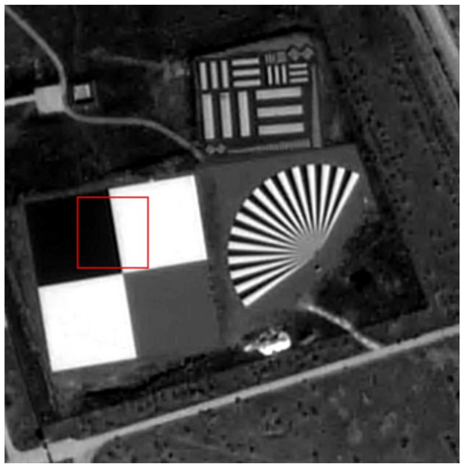
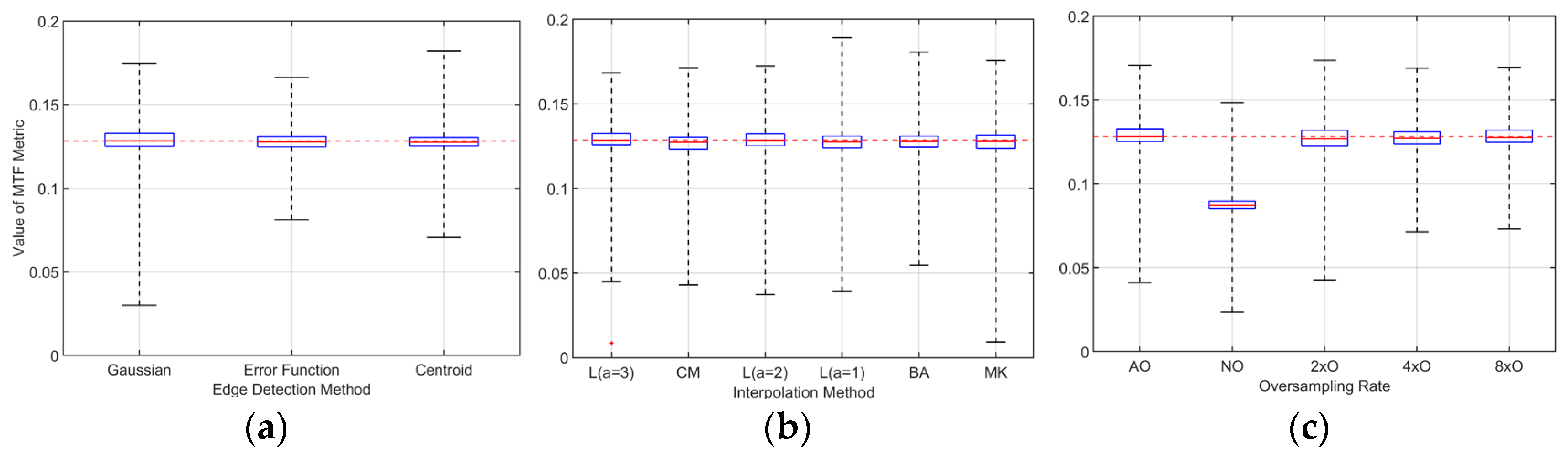
4.1. Process Analysis of Slanted-Edge Method

Based on the GF-2 optical satellite sensor parameters, the theoretical MTF is calculated as a reference value to evaluate the accuracy of the edge method. The parameters used are listed in

Table 2. GF-2 satellite sensor parameters for theoretical MTF estimations.

Parameter	Value of Each Channel
Diffraction wavelength/μm	PAN: 0.65	B1: 0.49	B2: 0.55	B3: 0.67	B4: 0.83
Sampling pixel size/μm	10	40
WFE/λrms	0.13
F-number	15
Focal length of optical system/m	7.8
Optical system aperture/mm	530
Field of view/°	2.1

, including the sampling pixel size, optical system focal length, F-number, optical system aperture, diffraction wavelength, etc. [41]. Assuming that ${MTF}_{amt}\left(v\right)=1$, taking the PAN band as an example, the MTF curves of various parts of the satellite optical system under different edge inclination angles are simulated based on Equations (1)–(3), as shown in Figure 4. The variation in $MT{F}_{det}$ with angle is more pronounced, likely due to the sampling degradation in different directions caused by the detector’s rectangular sampling [42].

When the satellite is on-orbit, there will definitely be some differences between its along-track MTF and cross-track MTF. It should be noted that since only the optical system parameters of the satellite were considered in the simulation images, without taking the orbit parameters into account, the MTF results based on the simulation images in this paper are the same in both along-track and cross-track directions. Taking the 7° angle as an example, the simulated static MTF values at Nyquist frequency in the cross-track and along-track directions are both 0.1283, which is consistent with the static MTF of the GF-2 satellite observed in the laboratory for the panchromatic spectrum [41]. In the evaluation and analysis of the MTF, particular attention was paid to edge detection methods, oversampling rates, and interpolation methods, as these three factors are critical in determining the accuracy, stability, and computational efficiency of the results. Edge detection serves as a foundational step that directly impacts the extraction and fitting of edge features, thereby determining the fidelity of the MTF curve. Similarly, the appropriate selection of oversampling rates enables a balance between enhancing the MTF calculation accuracy and minimizing excessive computational overhead. Finally, the interpolation methods significantly affect the retention of high-frequency details and the overall precision of the MTF results.

4.1.1. Edge Detection Method

Accurate edge detection and edge location determination are crucial for the calculation of the edge method. The essence of different edge detection methods is to extract the edge pixels with discontinuous gray levels in the image. The error function method was selected to represent the parametric method, and the commonly used Gaussian function and centroid detection method were selected as the non-parametric methods for comparative analysis. In the process of calculation based on the error function, assigning weights that are inversely proportional to the error of each sample point to the data can ensure the effective fitting of the sample data. The weight $w_i$ is defined as follows:

$$w_i=w_{F}exp\left(-{\displaystyle \frac{{\left(x_i-CenG\right)}^2}{2(3\Sigma {)}^2}}\right)+1$$

(8)

where $w_F$ is a scaling factor; $\Sigma$ is the average standard deviation of the gray gradient distribution in each row; $CenG$ is the center position of the gray gradient distribution.

Figure 5 shows the variation in the MTF values obtained through edge detection using the Gaussian fitting method (Figure 5a), error fitting method (Figure 5b), and centroid detection method (Figure 5c) in the polar coordinate, within the frequency range of 0–0.6 lp/pix and the edge inclination range of 0.5–44.5°. Different colors represent different MTF values. It can be seen that as the angle increases, the MTF shows a significant downward trend, especially when it is greater than 15°. According to the results of the three detection methods, a low edge slant angle (approximately less than 3°) will result in insufficient sampling and the inability to calculate an effective MTF; while edge slant angles (approximately greater than 12°) that are too high may cause the signal to alias to some extent, resulting numerical hopping in the figure. Therefore, when calculating the MTF based on edge images, it is advisable to control the edge slant angle within a small angular range. In the small angle case, the Gaussian fitting method and error fitting method have high consistency, and the MTF values show a more synchronous robustness while the centroid detection method exhibits significantly more instability than the former two.

4.1.2. Oversampling Rate

In the process of obtaining the ESF, it is necessary to project each pixel in the edge image matrix along the direction of the edge line into a 1D array. The sampling bin of the projected data is sub-pixel and irregular. In the ISO 12233 standard, 1/4 of the original image bin, which is four times the sampling rate, is used to regularize the bin of the new 1D array. However, the underlying principle behind choosing a 4× oversampling rate is still unclear. Due to the periodic misalignment between the projection direction and the bin array, using a fixed integer oversampling rate might reduce the accuracy of MTF estimation [17]. In the calculations used in this article, a dynamic adaptive oversampling rate based on the maximum spectral component position was used. Based on the frequency distribution of the distance from each pixel to the edge line in the image matrix, the position was determined via the maximum frequency spectral amplitude at the frequency $f_n$, where $1/f_n$ is the adaptive bin. In the analysis of edge detection methods in Figure 4 of the previous section, dynamic adaptive oversampling rates were used, which can be compared with the results for the different fixed oversampling rates shown in Figure 6.

Figure 6 shows the distribution of different MTF values with oversampling rates and edge detection methods. The range of polar coordinates is the same as that shown in Figure 4, with a frequency axis range of 0–0.6 lp/pix and an edge inclination range of 0.5–44.5°. The four rows in the figure, from top to bottom, are the Gaussian fitting method, error fitting method, and centroid detection method. From left to right, the three columns are no oversampling, 2× oversampling, 4× oversampling, and 8× oversampling.

The results show that the MTF values are significantly lower than the real value at low sampling rates, and it is difficult to obtain effective MTF results at small angles. The main reason for this is that the high-frequency information of the image cannot be sufficiently captured at low sampling rates, resulting in an inability to accurately reflect the true resolving power of the system. Although a sampling rate that is 8× higher can capture the image details more accurately, its computational cost is higher, and it also introduces noise and overfitting problems, reducing the robustness of MTF calculations. From the comprehensive comparison of Figure 5 and Figure 6, it can be seen that the results of the adaptive oversampling are better. However, in the small angle range, the results of the 4× and 8× rates are also relatively stable, which is consistent with the conclusions regarding the adaptive oversample rate presented by Wu et al. [42].

4.1.3. Interpolation Method

After regularizing the bin with oversampling, the data in the 1D ESF array remain highly nonlinear. To facilitate derivative calculations and allow for the use of discrete Fourier transform, it is necessary to interpolate or resample ESF into a linear array and estimate and fill data points at equidistant locations to maintain the integrity and continuity of the data.

Table 3. Effect of interpolation method on MTF at a 7° edge inclination and the adaptive oversampling rate.

Interpolation Method	MTF (Nyquist) for Gaussian Fitting Method	MTF (Nyquist) for Fitting Error Function	MTF (Nyquist) for Centroid Detection Method
Lanczos (a = 3)	0.1283 *	0.1277	0.1275
Continuum magic	0.1275	0.1242	0.1256
Lanczos (a = 2)	0.1283	0.1276	0.1274
Lanczos (a = 1)	0.1277	0.1262	0.1268
Bin average	0.1279	0.1274	0.1274
Mitchell kernel	0.1280	0.1261	0.1266

* The theoretical estimate of the ${\mathit{MTF}}_{\mathit{sys}}\left(v\right)$ at a Nyquist frequency of 0.1283.

lists the MTF results based on the commonly used high-precision interpolation methods in remote sensing image processing at a 7° edge inclination, while Figure 7 illustrates the effect of these interpolation methods on the accuracy of the results at different inclinations. Based on the experimental results in Section 4.1.1 and Section 4.1.2, the Gaussian fitting method and adaptive oversampling rates were used to compare the interpolation methods. The range of values for the coordinate axis in the figure is the same as that in Figure 6. Lanczos is a convolutional interpolation method based on the use of the sinc function as the kernel function. Parameter a determines the window size of the kernel function to balance the need to maintain sufficient sharpness and the need to reduce ringing effects. With a = 3 and a = 2, this interpolation method preserves the image details, as shown in Figure 7a and Figure 7c, respectively, whereas performances with a = 1 are slightly inferior, as illustrated in Figure 7d. Compared to Lanczos, the continuum magic interpolation method, as depicted in Figure 7b, is a smoother and less oscillatory interpolation method, implying that the sharpness of the original data might be smoothed out, resulting in higher instability at high spatial frequencies. The Bin average interpolation method, shown in Figure 7e, interpolates new data points using the average value of nearby data points, with low precision but a relatively high computation speed. The Mitchell kernel interpolation method, demonstrated in Figure 7f, is a cubic interpolation method, which places more emphasis on data smoothness during interpolation. The results from six groups of simulation experiments show that the Lanczos interpolation data are closest to the original data distribution [43], achieving the best interpolation effect.

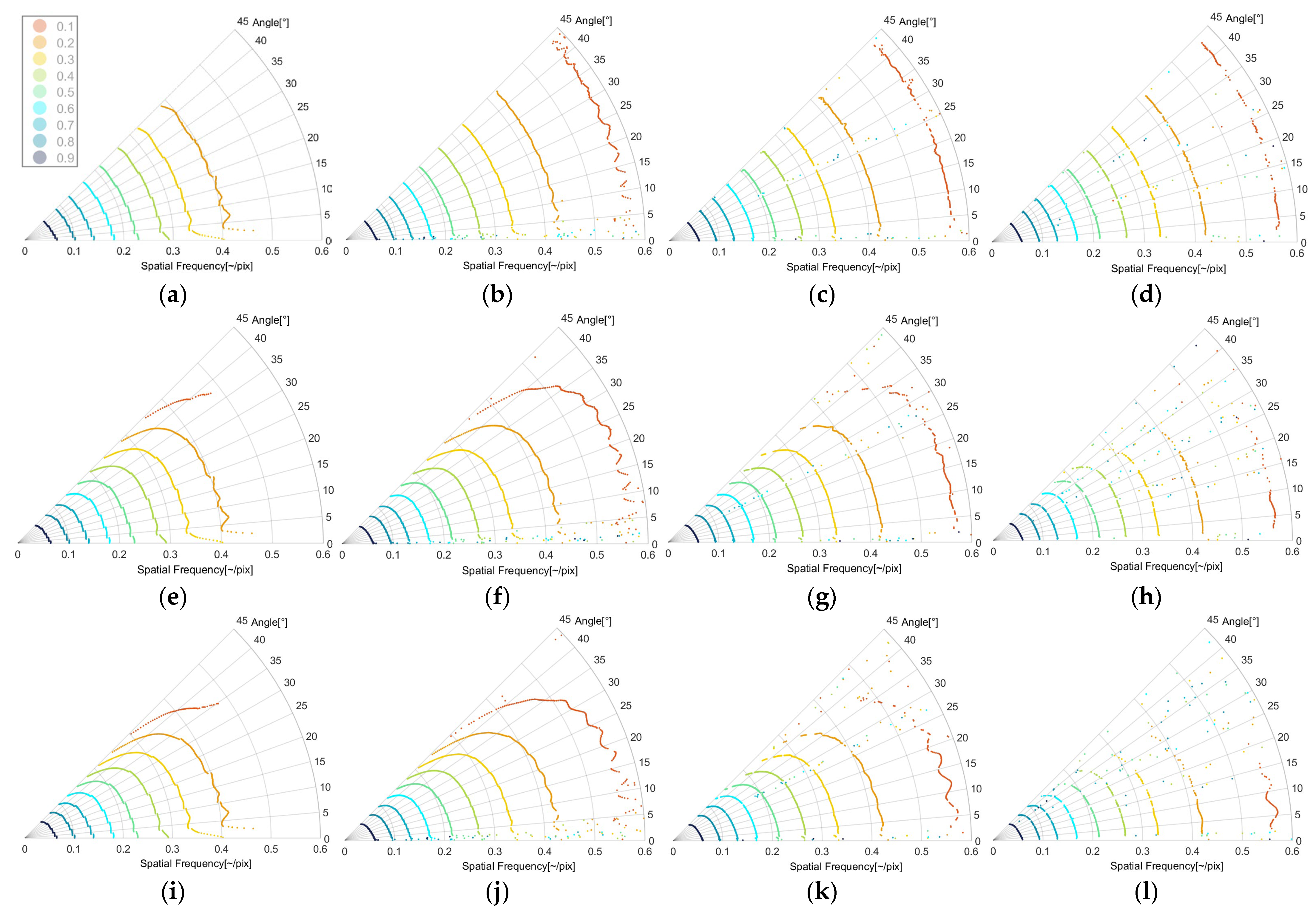
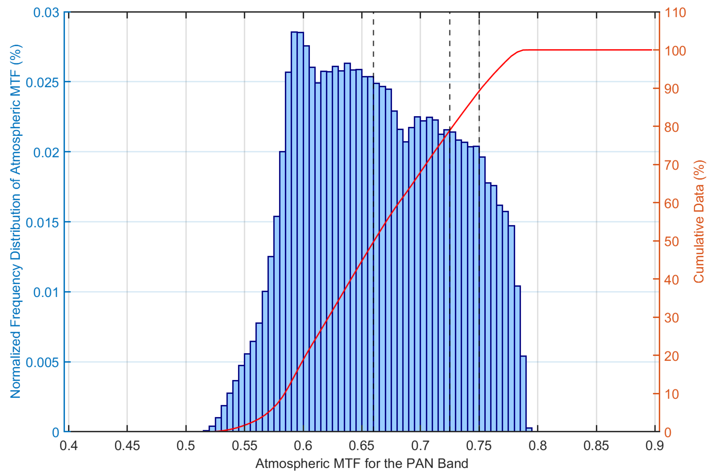
4.2. Analysis of Atmospheric Scattering and Absorption MTF

Haze weather can cause a higher proportion of light to scatter at small angles in the forward direction, resulting in blurry images, especially in long-range imaging [27]. Therefore, many satellite sensors choose cleaner locations during on-orbit MTF measurements to minimize the impact of atmosphere. Although the influence of atmospheric optical depth on long-range sensor imaging has been analyzed through experiments or simulations in some studies [27], there are few studies on the quantitative changes in atmospheric MTF during on-orbit measurements due to factors such as altitude, solar geometry, and satellite geometry. In order to analyze the influence of each factor on atmospheric MTF, this paper used the control variable method to calculate the atmospheric scattering and absorption MTF in sequence according to the flow in Figure 3. The analyzed variables include the SZA, VZA, relative azimuth angle (RAZ) calculated from the absolute difference between the solar azimuth angle and satellite azimuth angle, AOD, CWV, and altitude of the target (ALT). The atmospheric model was set as a user-defined type, inputting water vapor and ozone contents and using the vertical profile of the U.S. Standard Atmosphere (US62). Due to the minimal impact of ozone absorption on the spectral band of the GF-2 satellite, it was assumed to be an invariant in the analysis when using ground-based observations (listed in Table 1). The aerosol model was set as continental type based on the geographical and climate characteristics of the selected Baotou site. In the iterative calculation, the variables were cycled using the values in

Table 4. Simulation parameter settings of atmospheric and environmental factors.

Parameter Type	Value Ranges
Satellite Spectral Bands (nm)	PAN (450–900), B1 (450–520), B2 (520–600), B3 (630–690), and B4 (770–890)
SZA (°)	0:10:50 with a deviation of ±1
VZA (°)	0:10:50 with a deviation of ±1
RAZ (°)	0:10:180 with a deviation of ±1
AOD	0:0.1:0.5 with a deviation of ±0.005
CWV (g/cm2)	0:1:5 with a deviation of ±0.1
Altitude/ALT (km)	0:1:5 with a deviation of ±0.1

, and invariants were set using the satellite and ground parameters in Table 1. In order to verify the robustness of the influence of various factors on atmospheric scattering and absorption MTF, the deviation of each variable was also considered in the calculation process, including SZA with ±1° deviation, VZA with ±1° deviation, RAZ with ±1° deviation, AOD with ±0.005 deviation, CWV with ±0.1 g/cm² deviation, and ALT with ±0.1 km deviation. The quantitative changes in atmospheric scattering and absorption MTF at the Nyquist frequency are shown in Figure 8.

The results indicate that VZA, AOD, and ALT have a more significant impact on the atmospheric scattering and absorption MTF of GF-2 optical satellites in various bands, while SZA, RAZ, and CWV appear to have little effect on the atmospheric MTF. With the increase in AOD, the extinction effect of the atmosphere is enhanced and the atmospheric scattering and absorption MTF of each band shows a rapid downward trend (Figure 8a). With the increase in ALT, the atmospheric scattering and absorption MTF of each band shows a slow and slight upward trend (Figure 7d). When the VZA is less than 30°, the atmospheric scattering and absorption MTF of each band remains relatively stable; when VZA is greater than 30°, the atmospheric path observed by the satellite becomes longer, and the atmospheric scattering and absorption MTF rapidly declines (Figure 8c). The deviation added to each parameter does not affect the trend in the curve shown in Figure 7, indicating that the atmospheric scattering and absorption MTF is robust and non-random in its variation with these factors. Moreover, regardless of whether the impact is significant or insignificant, the order of atmospheric scattering and absorption MTF changes with the band changes remains unchanged, with the B1 band having the smallest value and the B4 band having the largest value. The reason for this is that, as the wavelength increases, the influence of the atmospheric scattering and absorption on each band gradually decreases.

5. Discussion

5.1. Error Analysis of Slanted-Edge Method

Based on the process analysis of the edge method presented in Section 4.1, it can be concluded that, in the calculation of the slanted-edge method, the employment of the Gaussian fitting method for edge detection, the adaptive oversampling rate, and the Lanczos (a = 3) interpolation method yields the closest result to the theoretical reference value. Considering the variability across experimental methods, repeated experiments were conducted to assess the distribution of MTF deviations caused by various factors in the calculation process and to verify the applicability of the above conclusions. Firstly, an ideal image with a slant angle of 7° was simulated. Then, by superimposing minimal noise on the image, separate sets of 1000 repetitive experiments were conducted for each edge detection method, oversampling rate, and interpolation method to obtain the distributions of MTF and ΔMTF. The results are shown in Figure 9.

Figure 9a–c present the MTF value distribution of 1000 repeated experiments using different edge detection methods, oversampling rates, and interpolation methods, respectively. The solid line in the middle of the box plot represents the median MTF value, with the top and bottom indicating the first and third quartiles of the MTF value, respectively. The red dashed line at 0.1283 represents the theoretical value of ${MTF}_{sys}$. From the maximum and minimum values of the box plots, the dispersion of Gaussian method in Figure 9a, Lanczos (a = 3) method in Figure 9b, and adaptive oversampling rate in Figure 9c are all moderate compared to other methods. Despite being slightly affected by noise, their MTF medians are almost the same as the theoretical values, indicating that these methods are relatively more accurate.

Figure 9d–f show the distribution of ΔMTF values for repeated experiments. In Figure 9d, the Gaussian fitting method shows an absolute error range from −0.0984 to 0.0464, with its median value closer to 0 than those obtained using the error fitting method and centroid detection method used for edge detection. When considering systematic errors, the error magnitude and distribution consistency of the Gaussian fitting method are more ideal. In Figure 9e, the Lanczos (a = 3) interpolation method has an average absolute error of −0.0001, which is closer to 0 than that obtained using other interpolation methods. The median is slightly negative-biased, but overall, the Lanczos (a = 3) interpolation method demonstrates the best performance in terms of measurement accuracy. In Figure 9f, the range of MTF results measured at different oversampling rates is relatively similar, with the largest variation and widest distribution observed for the 0× oversampling measurement values, spanning from −0.1045 to 0.0199. The average absolute error of the adaptive oversampling rate is nearly zero (0.0002), indicating the highest measurement accuracy among all methods. In comparison, the mean absolute errors for the 4× and 8× fixed oversampling rates are −0.0006 and −0.0003, respectively, with medians of −0.0009 and −0.0005. Although these fixed oversampling rates exhibit relatively low error magnitudes, they still fail to achieve the precision of the adaptive oversampling method. Furthermore, fixed oversampling rates slightly skew toward negative values and lack the dynamic adaptability of AO, making them prone to underperformance in more complex or non-uniform scenarios.

Therefore, for the on-orbit MTF measurement of the GF-2 satellite images, using the Gaussian fitting method for edge detection, adaptive oversampling rate and Lanczos (a = 3) interpolation methods can best reflect the characteristics of the edge data.

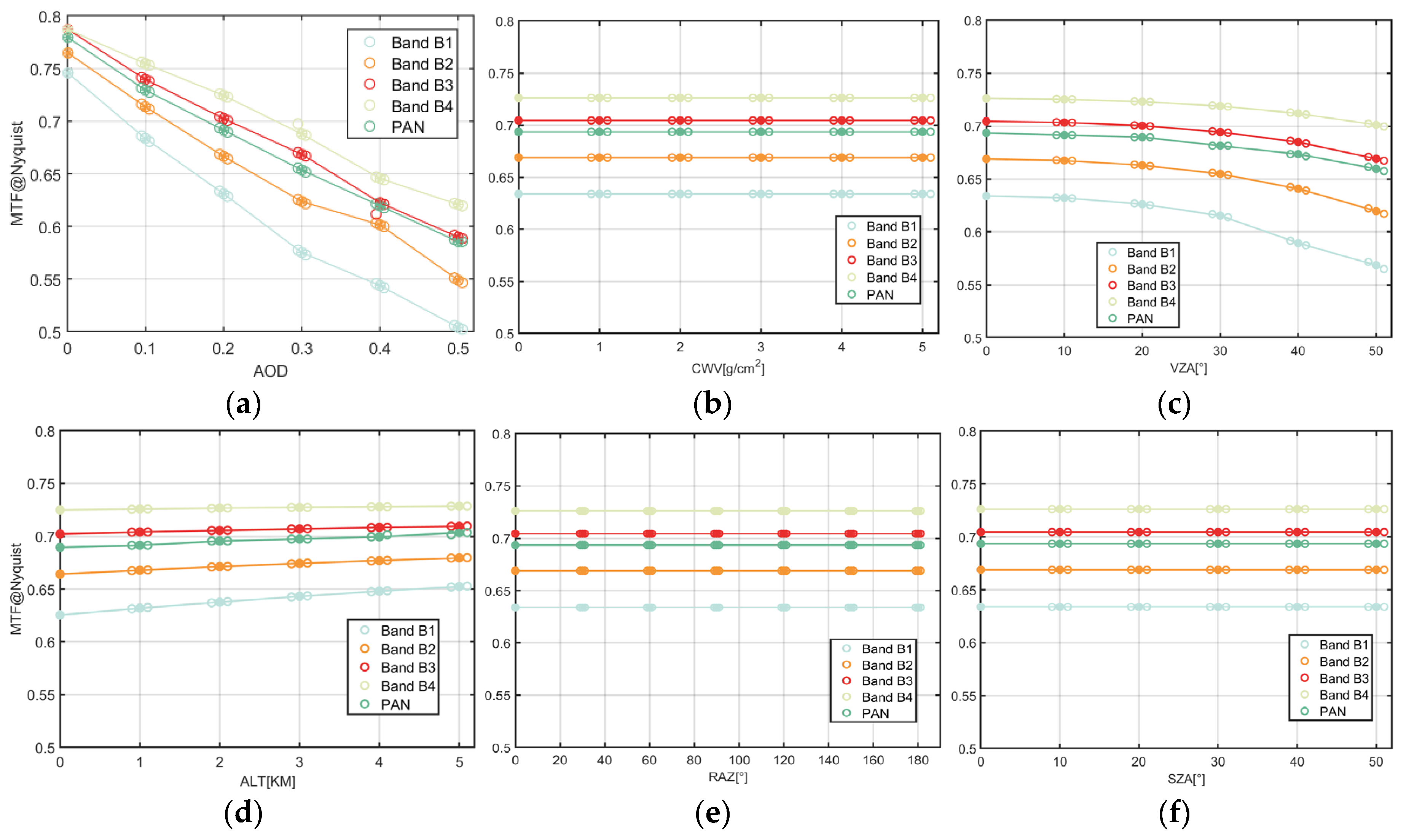
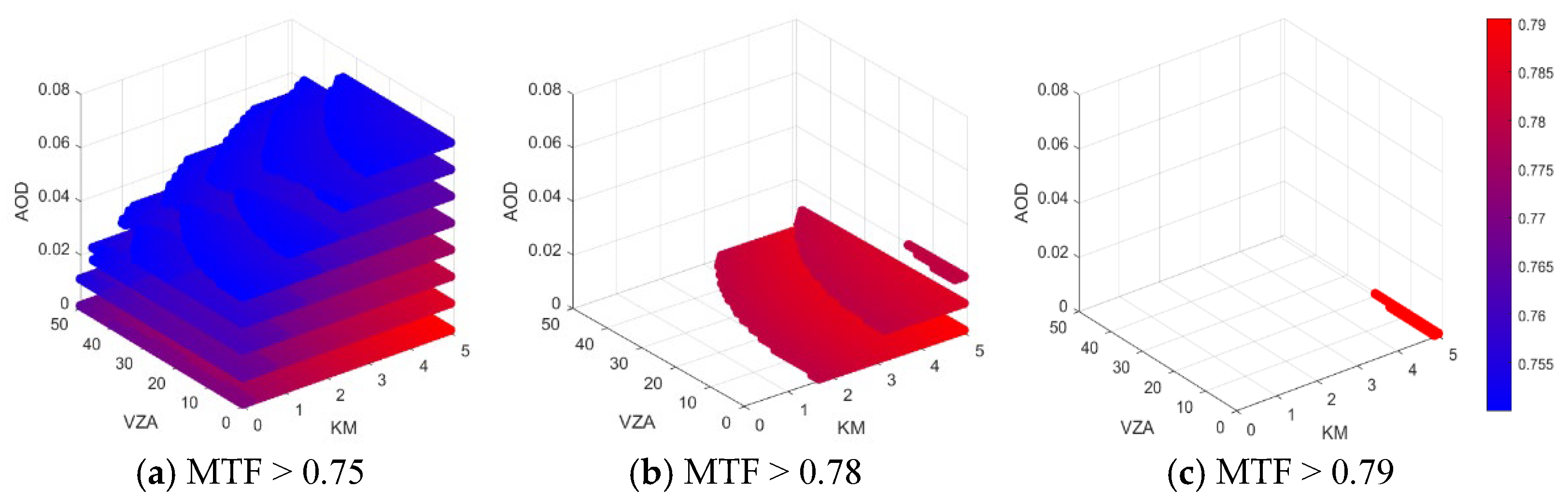
5.2. Analysis of Atmospheric Impact Factors

According to the previous analysis, the elements that have a greater impact on atmospheric scattering and absorption MTF during satellite on-orbit measurement are AOD, which is used to represent aerosol extinction, ALT at the test site, and VZA during satellite imaging. The increase in AOD corresponds to the increase in particulate matter in the atmosphere, leading to enhanced atmospheric scattering and resulting in blurry satellite images. VZA determines the length of the satellite observation path; the longer the path, the greater the influence of atmosphere. The change in ALT affects the results of atmospheric radiative transfer calculations during layer-by-layer integration in a stratified atmosphere. In order to ensure that each element analysis is not disturbed, the control variable method was used for calculation in Section 4.2. However, in actual satellite on-orbit testing applications, further attention should be paid to how to synergistically select the factors that have the main impact on atmospheric scattering and absorption MTF. Therefore, this paper takes a multi-dimensional data analysis approach to collaboratively consider the impact of changes in AOD, VZA, and ALT values on atmospheric MTF. The VZA range was set from 0 to 50° with a step of 1°; the AOD range was set from 0 to 0.5 with a step of 0.01; the ALT range was set from 0 to 5 km with a step of 0.1 km. Taking the PAN band of the GF-2 satellite sensor as an example, the quantitative calculation of atmospheric scattering and absorption MTF was still based on the flow in Figure 3 and a total of 132,651 data points were obtained. The other parameter values used in the calculation were all from the corresponding data in Table 1.

The results show that, under the known parameters, the numerical distribution range of atmospheric scattering and absorption MTF is 0.5174–0.7905, so the relative error of atmospheric scattering and absorption degradation can reach up to 34.56%. The histogram in Figure 10 presents the probability distribution of atmospheric scattering and the absorption MTF values for 132,651 data sets, with an interval of 0.02. The varying heights of the bar intuitively reflect the probability distribution of data points within each MTF value interval. It can be seen that within an MTF range of less than 0.59, as the MTF increases, the data probability rapidly increases, indicating that there are relatively few cases of very low atmospheric scattering and absorption MTF values. Although the numerical range of atmospheric scattering and absorption MTF is wide, the vast majority of the values were concentrated between approximately 0.59 and 0.75, and the probability was relatively consistent. When the value of atmospheric scattering and absorption MTF exceeds 0.75, its probability rapidly decreases. According to the data presented by the cumulative percentages curve, the atmospheric scattering and absorption MTF values corresponding to 50%, 80%, and 90% cumulative percentages were 0.6591, 0.7275, and 0.7520, respectively. This indicates that, in 90% of cases, the atmospheric scattering and absorption MTF is less than 0.7520.

Figure 11 shows the recommended threshold ranges for AOD, VZA, and ALT when the atmospheric scattering and absorption MTF is higher than 0.75, 0.78, and 0.79 under the set analysis conditions. The selection of the three MTF values was mainly based on a statistical analysis of the cumulative percentage of atmospheric scattering and absorption MTF values for 132,651 data sets presented in Figure 10. The cumulative percentages corresponding to MTFs of 0.75, 0.78, and 0.79 were approximately 90%, 98%, and 100%, respectively. It can be seen that the impact of the three elements on atmospheric scattering and absorption MTF has a non-regular distribution. The results indicate that, to meet the requirements of an atmospheric scattering and absorption MTF better than 0.75, the threshold range of the three elements is relatively loose, with an AOD within 0–0.08, VZA within 0–50°, and ALT within 0–5 km. To meet the requirement of an atmospheric scattering and absorption MTF better than 0.78, there are strict threshold ranges for the three elements, with an AOD of less than 0.02, VZA within 0–50°, and ALT greater than 1.7 km. To meet the requirement of an atmospheric scattering and absorption MTF of better than 0.79, AOD needs to be close to 0, VZA needs to be less than 20°, and ALT needs to be greater than 4.9 km. Therefore, the on-orbit testing of satellites should be conducted at sites with as low an AOD and as high an altitude as possible, as well as using a small satellite zenith angle.

Although a collaborative analysis of atmospheric scattering and absorption MTF was conducted for a GF-2 satellite within the specified parameter range, the conclusions can serve as a valuable reference for the assessment and testing of imaging quality of on-orbit satellites. It can offer directional guidance for the selection of meteorological condition, satellite attitude, and geographic location during the satellite on-orbit experiments and support the application of satellite on-orbit measurements and imaging quality assessments.

Finally, this paper mainly focused on the influence of atmospheric scattering and absorption on satellite image MTF when discussing atmospheric MTF, without an in-depth analysis of atmospheric turbulence. In optical communication links, atmospheric turbulence can cause fluctuations in the intensity and phase of the received light signal, resulting in image blurring [44]. However, due to the limitations of satellite resolution, the combination of adjacency effects and particulate small angle forward scatter is by far the dominant source of atmospheric blur in airborne and satellite imagery, so turbulence blur is usually neglected [27]. The impact of atmospheric turbulence on the satellite image MTF has not been thoroughly studied. In the future, with the continuous improvement in satellite resolution and the enhancement of meteorological data observation capabilities, in-depth research on the impact of atmospheric turbulence MTF is expected to lead to key breakthroughs in further improvements in image quality assessment accuracy.

6. Conclusions

This paper proposes a highly robust satellite on-orbit MTF measurement process. Based on the conventional edge-based method, refining and improving the key steps in the method, and conducting a simulation analysis and repeated experiments, the optimal calculation process that minimizes MTF error is obtained. The findings indicate that, for on-orbit MTF measurements of GF-2 satellite images, the Gaussian fitting method for edge detection, the adaptive oversampling rate, and the Lanczos (a = 3) interpolation method can most accurately express the image MTF.

Based on the sensor parameters of a GF-2 high-resolution satellite, a radiative transfer model was used to simulate satellite images with different atmospheric and imaging parameters. By comparing the MTF of these images with the MTF of the reference image, the influence of atmospheric scattering and absorption MTF on satellite on-orbit measurements was estimated and analyzed. The three most critical sensitive factors identified were aerosol optical depth, view zenith angle, and altitude. A scenario analysis using the PAN band of GF-2 satellite as an example showed that the atmospheric scattering and absorption MTF value is always below 0.7905, and in 90% of cases, it is less than 0.7520. This study addresses the issue that atmospheric MTF estimation based on statistical data often fails to consider sensor parameters and accurately reflect measurement errors in actual on-orbit scenarios. In addition, the results of a collaborative analysis of several main factors affecting atmospheric scattering and absorption MTF are provided, which can provide a reference for the selection of target site, observation geometry, and atmospheric conditions in satellite on-orbit MTF measurements.

References

1. Liao, J.; Gao, X. Dynamic MTF analysis and calculation of aerial camera. In Proceedings of the 5th International Symposium on Advanced Optical Manufacturing and Testing Technologies: Optoelectronic Materials and Devices for Detector, Imager, Display, and Energy Conversion Technology, Dalian, China, 26–29 April 2010; Volume 7658, pp. 288–294. [Google Scholar]
2. Leger, D.; Viallefont, F.; Hillairet, E.; Meygret, A. In-flight refocusing and MTF assessment of SPOT5 HRG and HRS cameras. In Proceedings of the International Symposium on Remote Sensing: Sensors, Systems, and Next-Generation Satellites VI, Crete, Greece, 23–27 September 2002; Volume 4881, pp. 224–231. [Google Scholar] [CrossRef]
3. Leger, D.; Viallefont, F.; Deliot, P.; Valorge, C. On-Orbit MTF Assessment of Satellite Cameras; Taylor & Francis Group: London, UK, 2004. [Google Scholar]
4. Bensebaa, K.; Banon, G.J.F.; Fonseca, L. On orbit spatial resolution estimation of CBERS-I CCD camera. In Proceedings of the Third International Conference on Image and Graphics (ICIG’04), Hong Kong, China, 18–20 December 2004; pp. 576–579. [Google Scholar] [CrossRef]
5. Bensebaa, K.; Banon, G.J.; Fonseca, L.M.; Erthal, G. On-orbit spatial resolution estimation of CBERS-2 imaging system using ideal edge target. In Signal Processing for Image Enhancement and Multimedia Processing; Springer Science & Business Media: Berlin/Heidelberg, Germany, 2008; pp. 37–48. [Google Scholar] [CrossRef]
6. Reulke, R.; Becker, S.; Haala, N.; Tempelmann, U. Determination and improvement of spatial resolution of the CCD-line-scanner system ADS40. ISPRS J. Photogramm. Remote Sens. 2006, 60, 81–90. [Google Scholar] [CrossRef]
7. Choi, T. IKONOS Satellite on Orbit Modulation Transfer Function (MTF) Measurement Using Edge and Pulse Method. Master’s Thesis, South Dakota State University, Brookings, SD, USA, 2002. [Google Scholar]
8. Rangaswamy, M.K. Quickbird II: Two-Dimensional On-Orbit Modulation Transfer Function Analysis Using Convex Mirror Array. Master’s Thesis, South Dakota State University, Brookings, SD, USA, 2003. [Google Scholar]
9. Kohm, K.; Louis, S. Modulation transfer function measurement method and results for the Orbview-3 high resolution imaging satellite. Proc. ISPRS 2004, 36, 12–23. [Google Scholar]
10. Tadono, T.; Shimada, M.; Watanabe, M.; Mukaida, A.; Kawamoto, S.; Imoto, N.; Yamashita, J. Initial results of calibration and validation for ALOS optical sensors. In Proceedings of the 2006 IEEE International Symposium on Geoscience and Remote Sensing, Denver, CO, USA, 31 July–4 August 2006; pp. 1643–1646. [Google Scholar] [CrossRef]
11. Jeong-Heon, S.; Dong-Han, L.; Sun-Gu, L.; Du-Ceon, S.; Soo-Young, P.; Hyo-Suk, L.; Hong-Yul, P. Modulation Transfer Function (MTF) Measurement For 1 m High Resolution Satellite Images such as KOMPSAT-2 Using Edge Function. In Proceedings of the KSRS Conference, Seoul, Republic of Korea, 29 July 2005; pp. 482–484. [Google Scholar]
12. Pagnutti, M.; Blonski, S.; Cramer, M.; Helder, D.; Holekamp, K.; Honkavaara, E.; Ryan, R. Targets, methods, and sites for assessing the in-flight spatial resolution of electro-optical data products. Can. J. Remote Sens. 2010, 36, 583–601. [Google Scholar] [CrossRef]
13. Wahballah, W.A.; El-Tohamy, F.; Bazan, T.M. A Survey and Trade-off-Study for Optical Remote Sensing Satellite Camera Design. In Proceedings of the 2020 12th International Conference on Electrical Engineering (ICEENG), Cairo, Egypt, 7–9 July 2020; pp. 298–305. [Google Scholar] [CrossRef]
14. Kameche, M.; Benmostefa, S. In-flight MTF stability assessment of ALSAT-2A satellite. Adv. Space Res. 2016, 58, 117–130. [Google Scholar] [CrossRef]
15. Masaoka, K.; Yamashita, T.; Nishida, Y.; Sugawara, M. Modified slanted-edge method and multidirectional modulation transfer function estimation. Opt. Express 2014, 22, 6040–6046. [Google Scholar] [CrossRef]
16. Masaoka, K. Accuracy and precision of edge-based modulation transfer function measurement for sampled imaging systems. IEEE Access 2018, 6, 41079–41086. [Google Scholar] [CrossRef]
17. Masaoka, K. Edge-based modulation transfer function measurement method using a variable oversampling ratio. Opt. Express 2021, 29, 37628–37638. [Google Scholar] [CrossRef]
18. Greer, P.B.; Van Doorn, T. Evaluation of an algorithm for the assessment of the MTF using an edge method. Med. Phys. 2000, 27, 2048–2059. [Google Scholar] [CrossRef]
19. Viallefont-Robinet, F.; Helder, D.; Fraisse, R.; Newbury, A.; van den Bergh, F.; Lee, D.; Saunier, S. Comparison of MTF measurements using edge method: Towards reference data set. Opt. Express 2018, 26, 33625–33648. [Google Scholar] [CrossRef]
20. Lutomirski, R.; Yura, H. Wave structure function and mutual coherence function of an optical wave in a turbulent atmosphere. J. Opt. Soc. Am. JOSA 1971, 61, 482–487. [Google Scholar] [CrossRef]
21. Kopeika, N. Spatial-frequency dependence of scattered background light: The atmospheric modulation transfer function resulting from aerosols. J. Opt. Soc. Am. JOSA 1982, 72, 548–551. [Google Scholar] [CrossRef]
22. Sadot, D.; Kopeika, N. Imaging through the atmosphere: Practical instrumentation-based theory and verification of aerosol modulation transfer function. J. Opt. Soc. Am. JOSA 1993, 10, 172–179. [Google Scholar] [CrossRef]
23. LeMaster, D.A.; Eismann, M.T. Impact of atmospheric aerosols on long range image quality. In Proceedings of the Infrared Imaging Systems: Design, Analysis, Modeling, and Testing XXIII, Baltimore, MD, USA, 23–27 April 2012; Volume 8355, pp. 102–111. [Google Scholar] [CrossRef]
24. Eismann, M.T.; LeMaster, D.A. Aerosol modulation transfer function model for passive long-range imaging over a nonuniform atmospheric path. Opt. Eng. 2013, 52, 046201. [Google Scholar] [CrossRef]
25. Wells, W.H. Loss of Resolution in Water as a Result of Multiple Small-Angle Scattering. J. Opt. Soc. Am. 1969, 59, 686–691. [Google Scholar] [CrossRef]
26. Steve, B.; Ronald, D.; Gerald, H.; Norman, S.K.; Arkadi, Z. Effects of aerosol modulation transfer function on target identification. Opt. Eng. 2020, 59, 073103. [Google Scholar]
27. Norman, S.K.; Arkadi, Z.; Yitzhak, Y. Aerosol MTF revisited. In Proceedings of the Infrared Imaging Systems: Design, Analysis, Modeling, and Testing XXV, Baltimore, MD, USA, 5–9 May 2014; Volume 9071, pp. 409–422. [Google Scholar] [CrossRef]
28. Li, C.; Tang, L.; Ma, L.; Zhou, Y.; Gao, C.; Wang, N.; Li, X.; Wang, X.; Zhu, X. Comprehensive calibration and validation site for information remote sensing. In Proceedings of the International Archives of the Photogrammetry, Remote Sensing and Spatial Information Sciences, Berlin, Germany, 11–15 May 2015; Volume XL-7/W3, pp. 1233–1240. [Google Scholar] [CrossRef]
29. Zhou, Y.; Li, C.; Tang, L.; Ma, L.; Wang, Q.; Liu, Q. A Permanent bar pattern distributed target for microwave image resolution analysis. IEEE Geosci. Remote Sens. Lett. 2017, 14, 164–168. [Google Scholar] [CrossRef]
30. Holben, B.N.; Eck, T.; Slutsker, I.a.; Tanré, D.; Buis, J.; Setzer, A.; Vermote, E.; Reagan, J.A.; Kaufman, Y.; Nakajima, T. AERONET—A federated instrument network and data archive for aerosol characterization. Remote Sens. Environ. 1998, 66, 1–16. [Google Scholar] [CrossRef]
31. Li, C.; Ma, L.; Tang, L.; Gao, C.; Qian, Y.; Wang, N.; Wang, X. A comprehensive calibration site for high resolution remote sensors dedicated to quantitative remote sensing and its applications. Natl. Remote Sens. Bull. 2021, 25, 198–219. [Google Scholar] [CrossRef]
32. ISO 12233:2023; Photography–Electronic Still Picture Imaging–Resolution and Spatial Frequency Responses. International Organization for Standardization: Geneva, Switzerland, 2023.
33. Abolghasemi, M.; Abbasi-Moghadam, D. Design and performance evaluation of the imaging payload for a remote sensing satellite. Opt. Laser Technol. 2012, 44, 2418–2426. [Google Scholar] [CrossRef]
34. Zhang, F.; Zhang, Y.; Deng, Q.; Cheng, Z.; Zhu, B. Modeling and Simulation of Electro-Optical Imaging Systems Based on MTF. Laser Infrared 2015, 45, 549–554. [Google Scholar]
35. Yang, B.; Cao, D. Technological Innovations and Insights of the “Gaofen-2” Satellite High-Resolution Camera. Aerosp. Return Remote Sens. 2015, 36, 10–15. [Google Scholar]
36. Chazallet, F.; Glasser, J. Theoretical bases and measurement of the MTF of integrated image sensors. In Proceedings of the Image Quality: An Overview, Arlington, VA, USA, 10–12 April 1985; Volume 0549, pp. 131–144. [Google Scholar] [CrossRef]
37. Li, X.; Jiang, X.; Zhou, C.; Gao, C.; Xi, X. An analysis of the knife-edge method for on-orbit MTF estimation of optical sensors. Int. J. Remote Sens. 2010, 31, 4995–5010. [Google Scholar] [CrossRef]
38. Kotchenova, S.Y.; Vermote, E.F.; Matarrese, R.; Klemm, F.J. Validation of a vector version of the 6S radiative transfer code for atmospheric correction of satellite data. Part I: Path radiance. Appl. Opt. 2006, 45, 6762–6774. [Google Scholar] [CrossRef]
39. Vermote, E.F.; Tanre, D.; Deuze, J.L.; Herman, M.; Morcette, J.-J. Second Simulation of the Satellite Signal in the Solar Spectrum, 6S: An overview. IEEE Trans. Geosci. Remote Sens. 1997, 35, 675–686. [Google Scholar] [CrossRef]
40. Richter, R.; Bachmann, M.; Dorigo, W.; Muller, A. Influence of the Adjacency Effect on Ground Reflectance Measurements. IEEE Geosci. Remote Sens. Lett. 2006, 3, 565–569. [Google Scholar] [CrossRef]
41. Pan, T. Technical characteristics of the Gaofen-2 Satellite. Aerospace China. 2015, 1, 3–9. [Google Scholar]
42. Wu, Y.; Xu, W.; Piao, Y.; Yue, W. Analysis of edge method accuracy and practical multidirectional modulation transfer function measurement. Appl. Sci. 2022, 12, 12748. [Google Scholar] [CrossRef]
43. Haefner, D.P. MTF measurements, identifying bias, and estimating uncertainty. In Proceedings of the Infrared Imaging Systems: Design, Analysis, Modeling, and Testing XXIX, Orlando, FL, USA, 17–18 April 2018; pp. 54–68. [Google Scholar]
44. Arkadi, Z.; Ephim, G.; Shlomi, A.; Norman, S.K. Kolmogorov and non-Kolmogorov turbulence and its effects on optical communication links. In Proceedings of the Free-Space Laser Communications VII, San Diego, CA, USA, 26–30 August 2007; Volume 6709, pp. 173–184. [Google Scholar] [CrossRef]
Figure 1. The PAN band image of the GF-2 satellite on 24 October 2021 at the Baotou site.
Remotesensing 16 04676 g001
Figure 2. Overall flowchart of this study.
Remotesensing 16 04676 g002
Figure 3. Flow chart of the quantitative calculation of atmospheric effects based on the atmospheric radiation transfer model.
Remotesensing 16 04676 g003
Figure 4. Frequency variations in (a) system MTF, (b) detector MTF, (c) aberration ATF, and (d) diffraction-limited optics OTF in the PAN band of the GF2 satellite for edge tilt angles of 0.5–44.5°.
Remotesensing 16 04676 g004
Figure 5. Variation in MTF in polar coordinates at edge inclination angles of 0.5–44.5°, with angular intervals of 0.2°, where (a) is the case of the adaptive oversampling rate under the Gaussian fitting method, (b) is the adaptive oversampling rate under the error fitting method, and (c) is the adaptive oversampling rate under the centroid detection method.
Remotesensing 16 04676 g005
Figure 6. Group diagram of the effect of doubling rate on MTF, where (ad) are the Gaussian fitting method, (eh) are the error fitting method, and (il) are the centroid detection fitting method. The first column of each row of images represents the case of no oversampling, the second column represents the case of 2× oversampling, the third column represents the case of 4× oversampling, and the fourth column represents the case of 8×oversampling.
Remotesensing 16 04676 g006
Figure 7. Group diagram of the effect of interpolation methods on MTF, where (a) is the Lanczos (a = 3) interpolation method, (b) is the continuum magic interpolation method, (c) is the Lanczos (a = 2) interpolation method, (d) is the f Lanczos (a = 1) interpolation method, (e) is the Bin average interpolation method, and (f) is the Mitchell kernel interpolation method.
Remotesensing 16 04676 g007
Figure 8. Group diagram of the results of atmospheric scattering and absorption MTF variations in various bands calculated based on satellite images, where (a) AOD, (b) CWV, (c) SZA, (d) ALT, (e) RAZ, and (f) SZA.
Remotesensing 16 04676 g008
Figure 9. (a) The distribution of MTF values of different edge detection methods, (b) the distribution of MTF values of different interpolation methods, and (c) the distribution of MTF values for different oversampling rates. (d) The distribution of ΔMTF values of different edge detection methods, (e) the distribution of ΔMTF values of different interpolation methods, and (f) the distribution of ΔMTF values for different oversampling rates. For (b) and (e), Lanczos (a = 3), Continuum magic, Lanczos (a = 2), Lanczos (a = 1), Bin average, and Mitchell kernel are abbreviated, respectively, as L (a = 3), CM, L (a = 2), L (a = 1), BA, MK; for (c) and (f), adaptive oversampling, no oversampling, 2× oversampling, 4× oversampling, and 8× oversampling is abbreviated, respectively, as AO, NO, 2×O, 4×O, 8×O. The red solid line in the middle of the box plot represents the median MTF value, the blue lines at the top and bottom respectively indicate the first and third quartiles of the MTF value, and the red dashed line at 0.1283 indicates the theoretical value of M T F s y s .
Remotesensing 16 04676 g009aRemotesensing 16 04676 g009b
Figure 10. Histogram of the atmospheric scattering and absorption MTF for the PAN band, accompanied by a cumulative data curve. Three vertical black dashed lines indicate the positions at which the cumulative percentages reach 50%, 80%, and 90%, respectively.
Remotesensing 16 04676 g010
Figure 11. Group diagram illustrating ranges of atmospheric conditions that satisfy the different requirements for atmospheric impact, including (a) an atmospheric scattering and absorption MTF above 0.75, (b) an atmospheric scattering and absorption MTF above 0.78, and (c) an atmospheric scattering and absorption MTF above 0.79, depicted in three-dimensional positions.
Remotesensing 16 04676 g011