

Few-Shot Metric Learning with Time-Frequency Fusion for Specific Emitter Identification


Abstract

1. Introduction
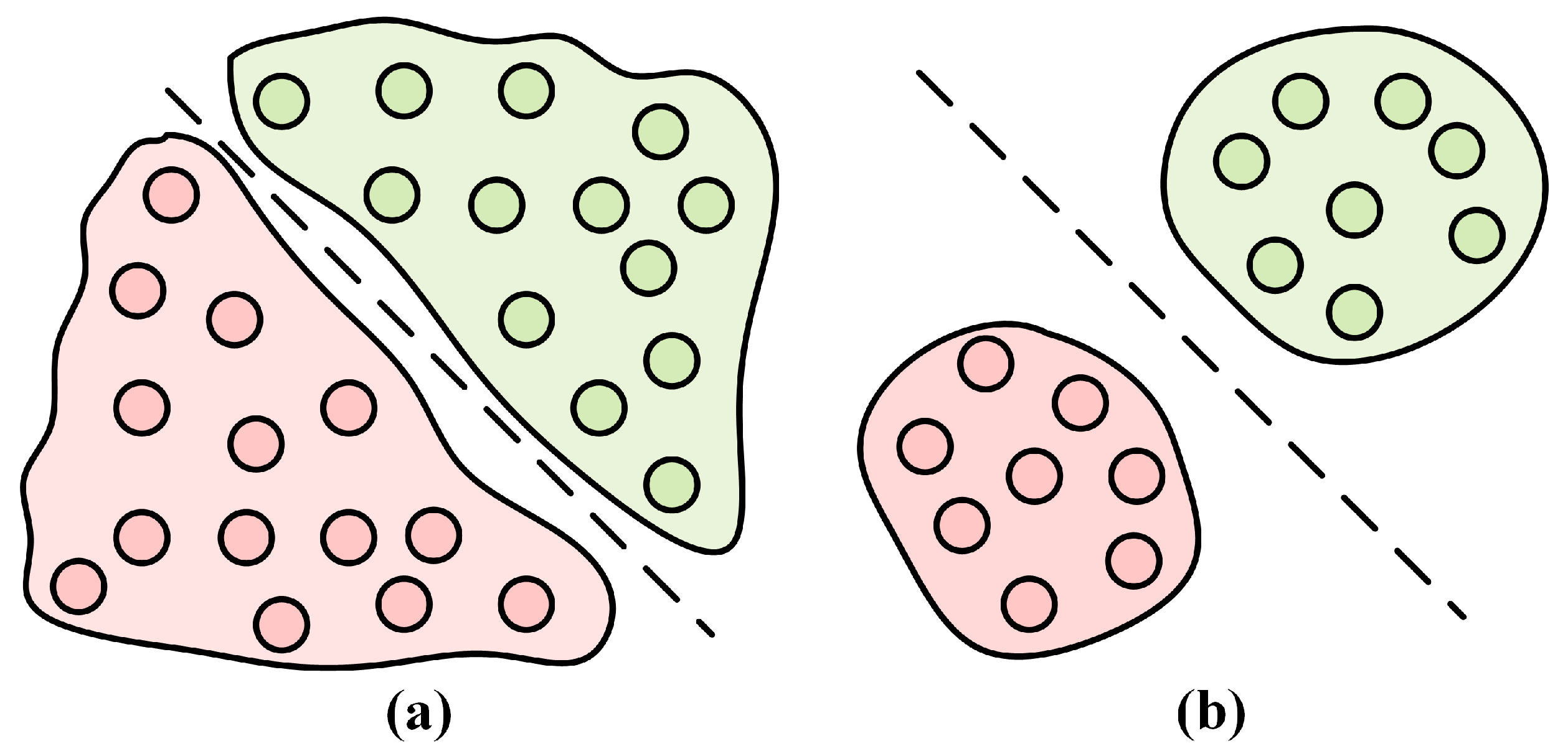
- A metric learning-based feature embedding scheme is proposed, aimed at extracting generalized and discriminative features, ensuring the most accurate representation of the embedding space while simultaneously maximizing inter-category distances and minimizing intra-category distances. This strategy has demonstrated superior performance, particularly in small sample tasks.
- The fusion of time-domain and frequency-domain information based on the attention mechanism is introduced, effectively exploiting the multi-view features of the signal. This method significantly enhances the quality of the extracted RF fingerprints.
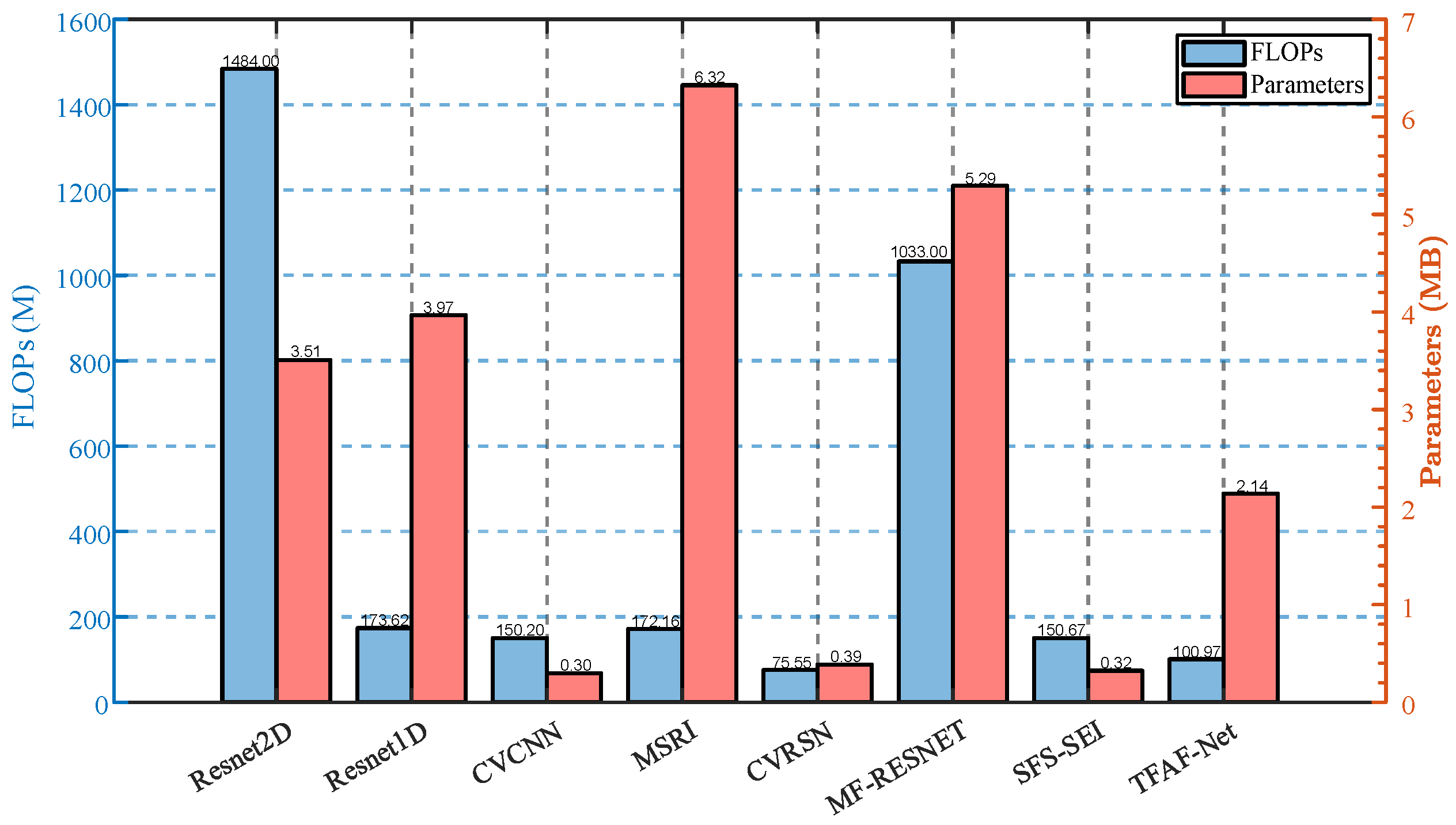
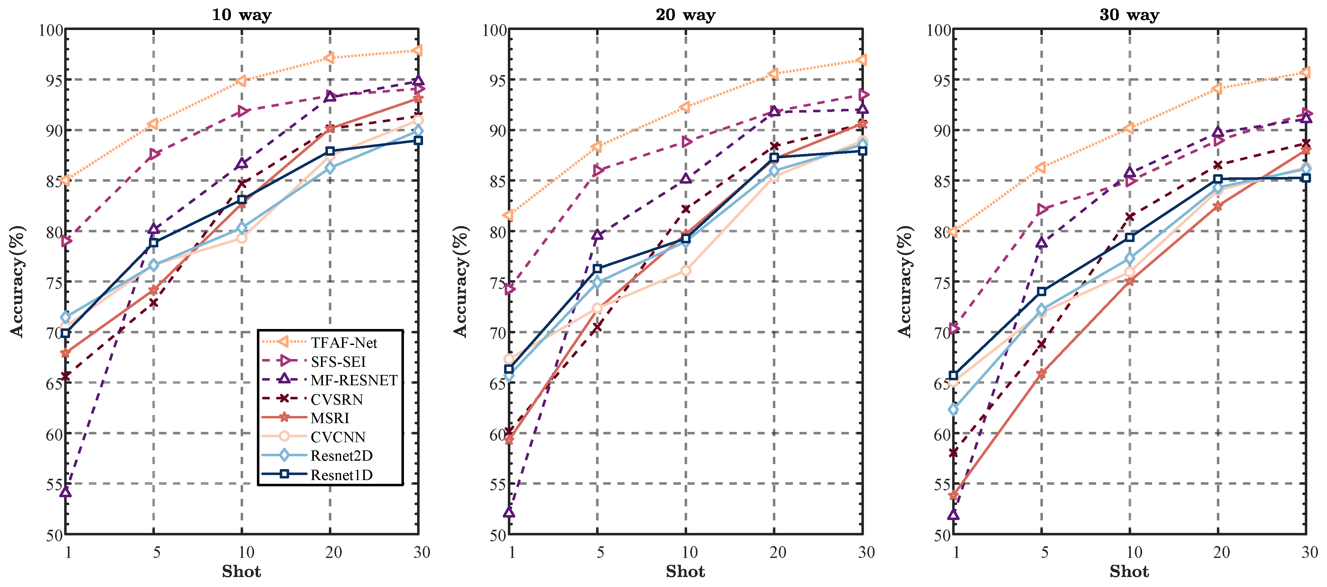
- The proposed SEI method is evaluated on an open-source large-scale real ADS-B dataset and an open-source Wi-Fi dataset, and compared with multiple existing SEI methods, including FS-SEI approaches. Results demonstrate that the proposed approach achieves state-of-the-art recognition performance, thanks to its architectural design that maximizes effectiveness while maintaining reduced parameters and complexity.
2. Related Work
2.1. Traditional SEI Methods
2.2. DL-Based SEI Methods
2.3. Few-Shot Learning in SEI
- Data Augmentation (DA): The DA-based methods aim to expand the training dataset by adding equivalent samples, thus overcoming the problem of insufficient training samples. Zhang et al. [20] proposed a DA-aided FSL method to improve the performance of SEI under limited sample conditions. This method is validated using automatic dependent surveillance–broadcast signals and introduces four DA techniques—flip, rotation, shift, and noise addition—to enhance the diversity of the training dataset and mitigate overfitting in small sample scenarios. Furthermore, the DA-based methods rely only on task-specific data, unlike other methods that leverage auxiliary data.
- Generative Model (GM): GM-based methods, such as autoencoders or GANs, are used to extract strong features from data. These features are capable of accurately representing and reconstructing the original samples. Yao et al. [21] introduced a novel approach to SEI using a FSL framework based on an Asymmetric Masked Auto-Encoder (AMAE). It addresses the challenge of identifying emitters with limited labeled samples by leveraging abundant unlabeled data for pre-training. The AMAE effectively extracts RFF features through a unique masking strategy, enhancing the model’s ability to learn meaningful representations. Compared to the Metric Model, GM may suffer from mode collapse and training instability issues common in GAN training.
- Metric Model (MM): Metric methods are grounded in the principles of “learning to compare” or “learning to measure”. These methods focus on developing representations that enable the evaluation and quantification of similarity among different samples. By learning an appropriate distance metric, these methods facilitate the classification, clustering, and retrieval of data points based on their inherent characteristics. Wu et al. [22] proposed an innovative open-set SEI method utilizing a Siamese Network. Their approach integrates unsupervised learning, clustering loss, and reconstruction loss during the training process to ensure comprehensive feature extraction. This methodology enhances the discrimination between known and unknown classes. By leveraging the Siamese Network, the method effectively measures the similarity between signal features, facilitating robust open set identification. Wang et al. [23] presented a novel FS-SEI method using interpolative metric learning (InterML). The proposed InterML method addresses these issues by eliminating the need for auxiliary data and improving generalization through interpolation and metric learning, enhancing identification accuracy and feature discriminability, particularly in FS settings.
- Meta Model (MEM): The core concept of meta methods is “learning to learn.” Meta-learning serves as an optimization approach aimed at enhancing the generalization capability of neural networks across various tasks. Yang et al. [24] proposed an SEI approach utilizing model-agnostic meta-learning, which achieved high accuracy with limited labeled samples and allowed for adaptation to new tasks without extensive retraining. Unlike MM, MeM may require careful task design and suffer from optimization challenges in meta-learning.
3. Signal Model and Problem Formulation
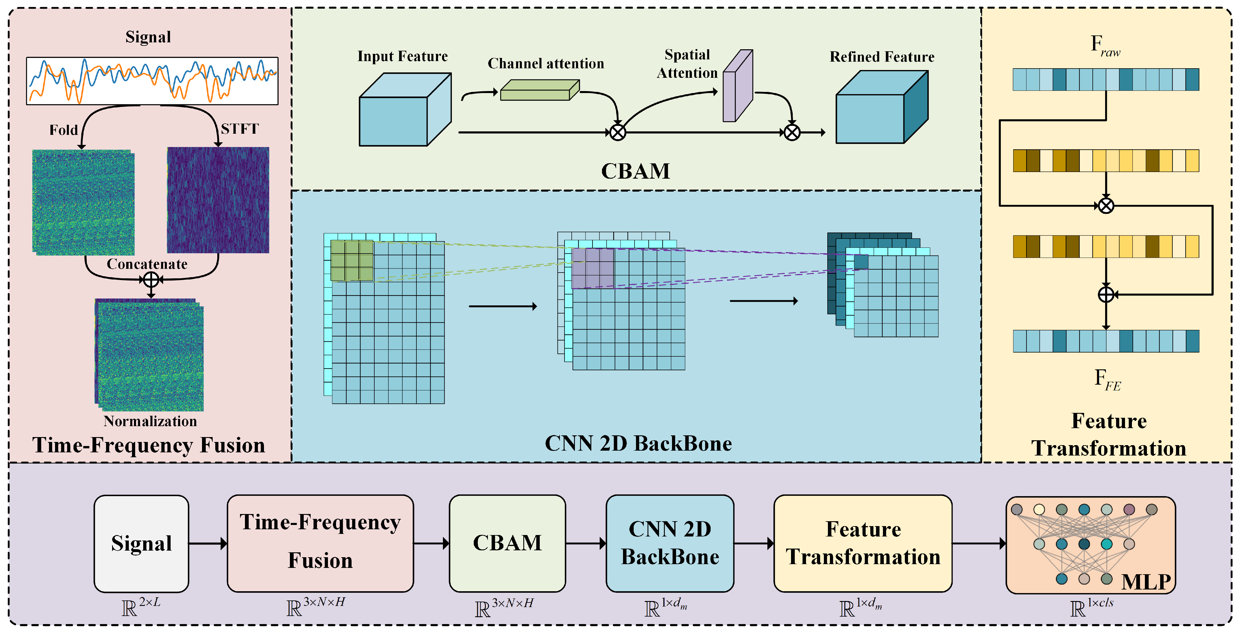
4. Methodology
4.1. Time-Frequency Representations
4.2. Time-Frequency Fusion
4.3. Time-Frequency Feature Refine
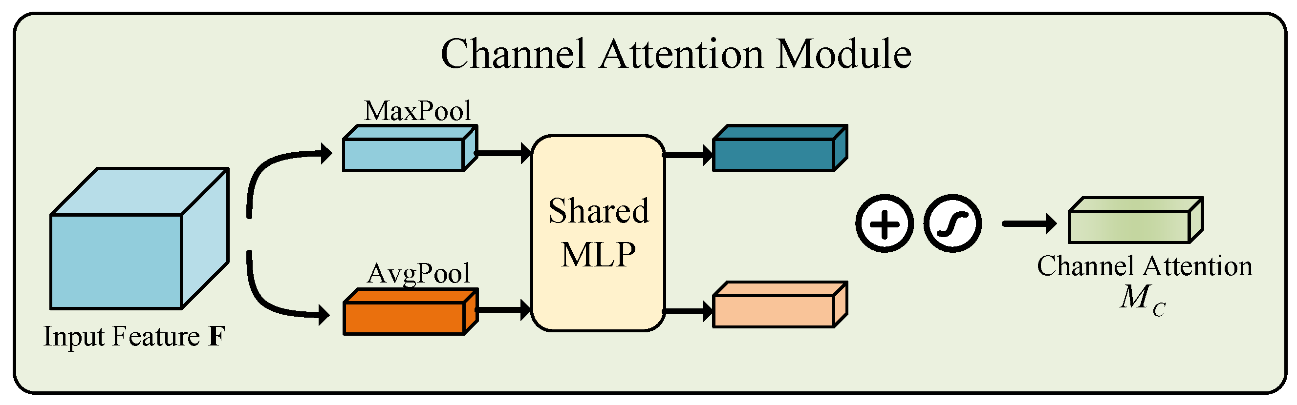
4.3.1. Channel Attention Module
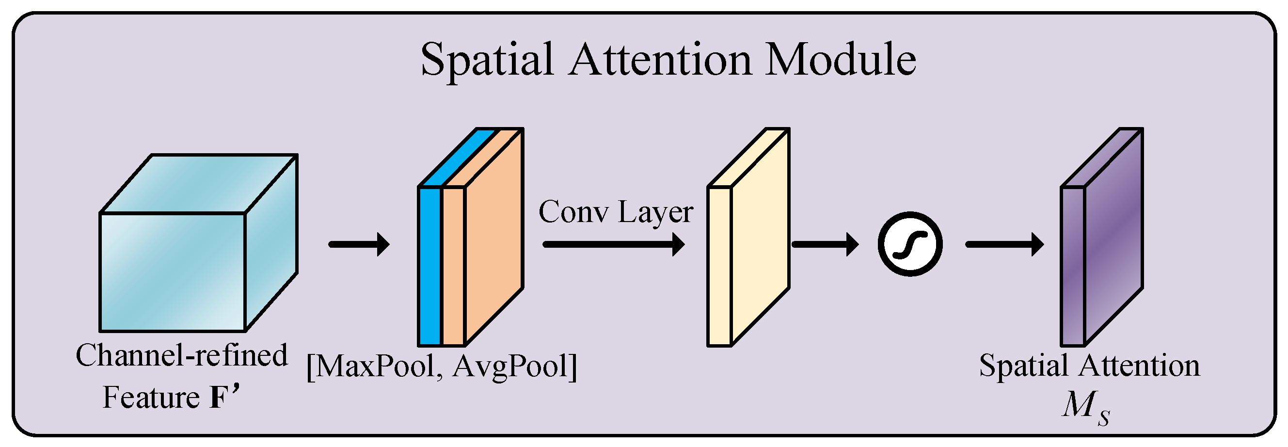
4.3.2. Spatial Attention Module
4.4. Loss Function Based on Metric Learning
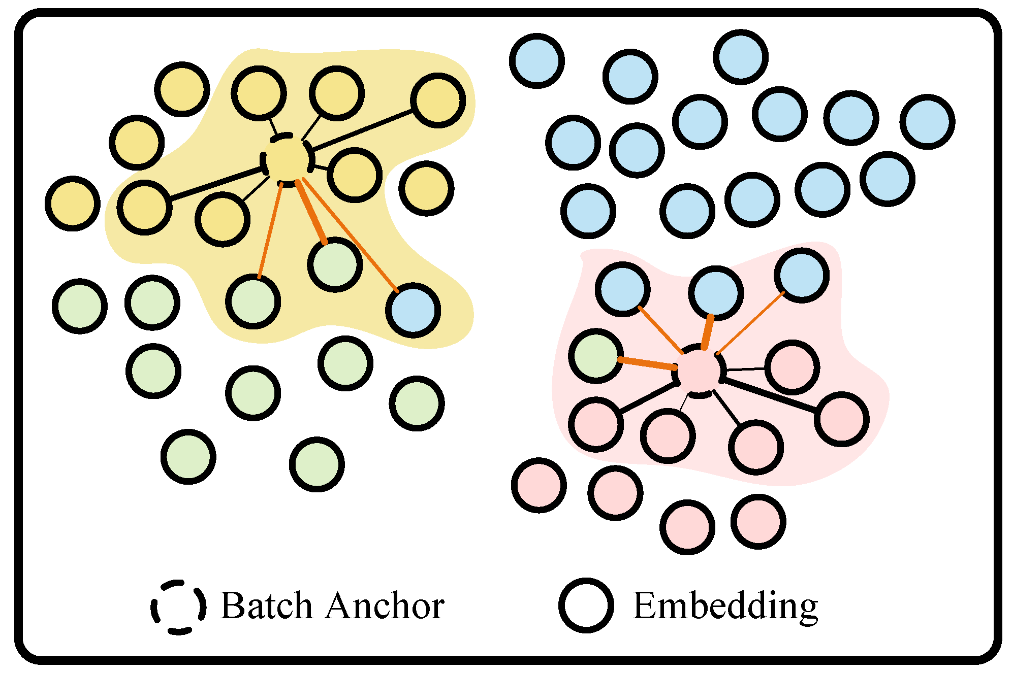
4.4.1. PA Loss
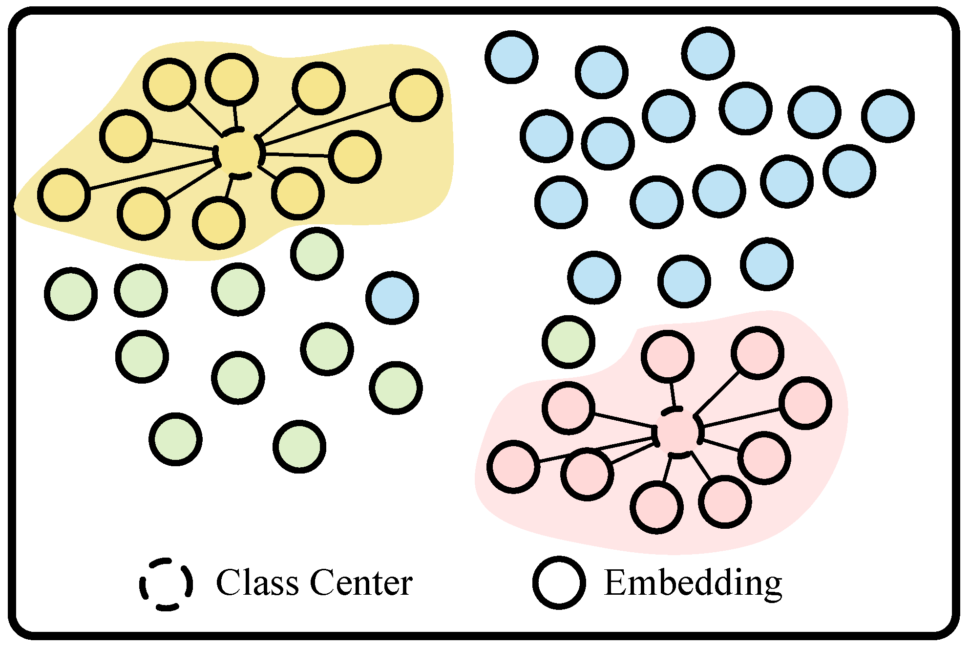
4.4.2. CT Loss
4.4.3. Cross-Entropy Loss
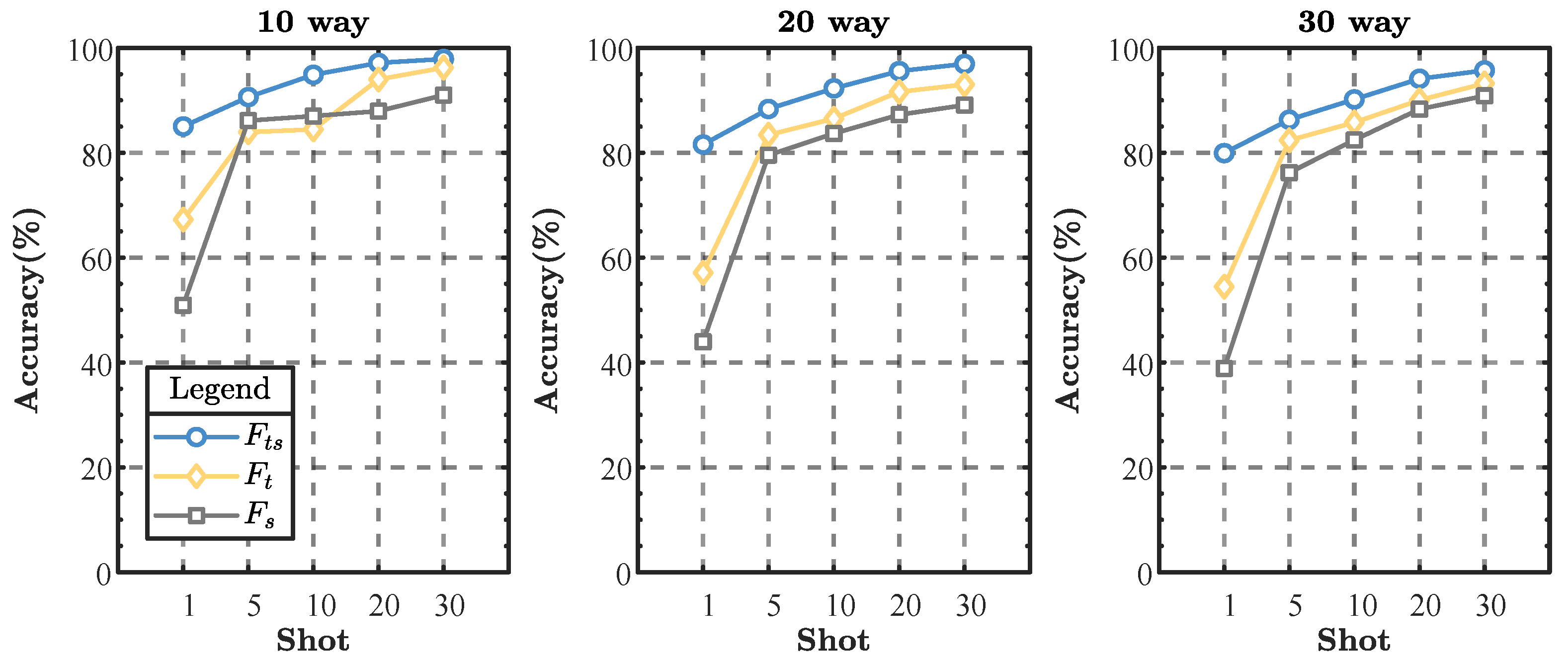
4.5. Feature Transformation
5. Experiment and Analysis
5.1. Dataset
5.2. Experimental Details
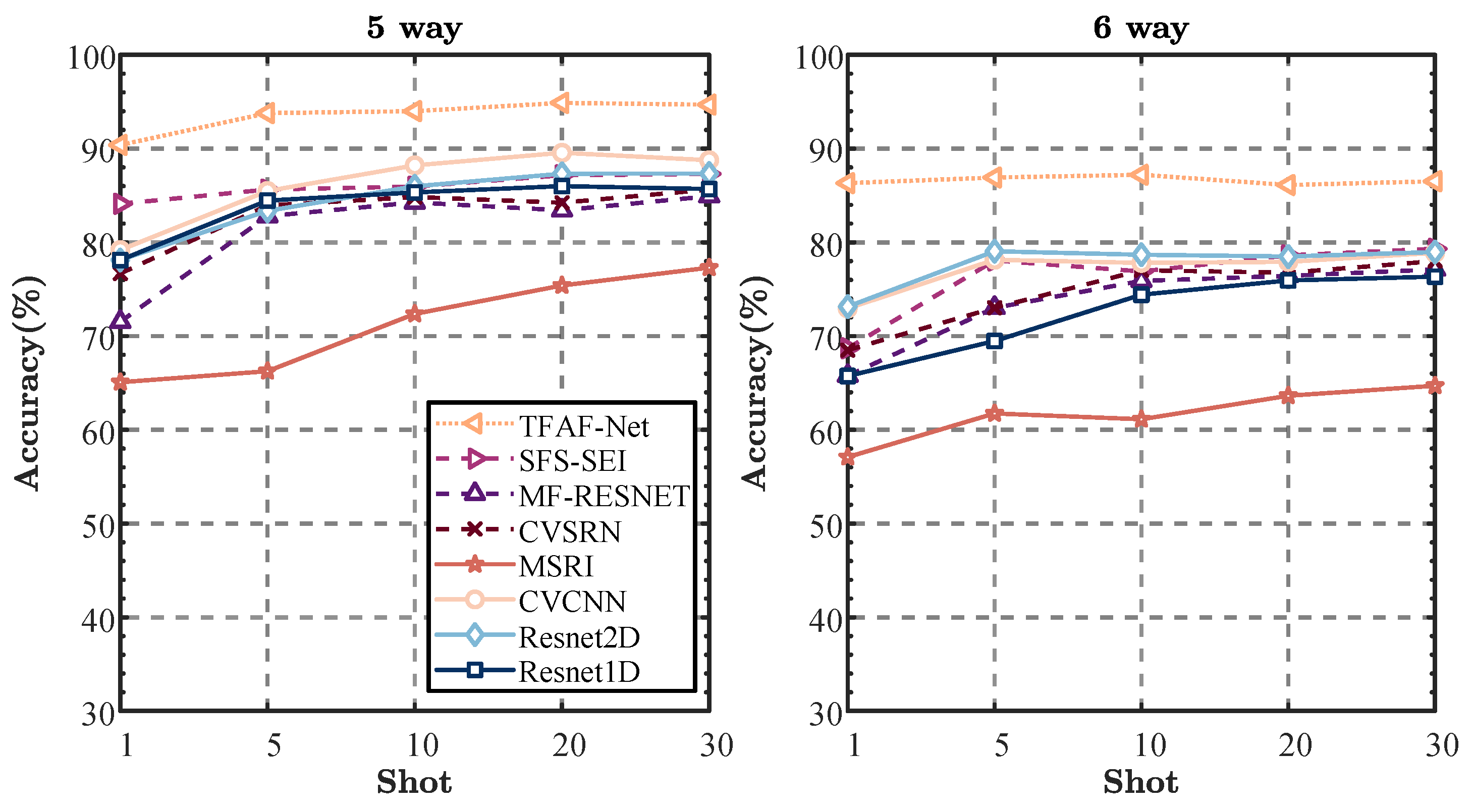
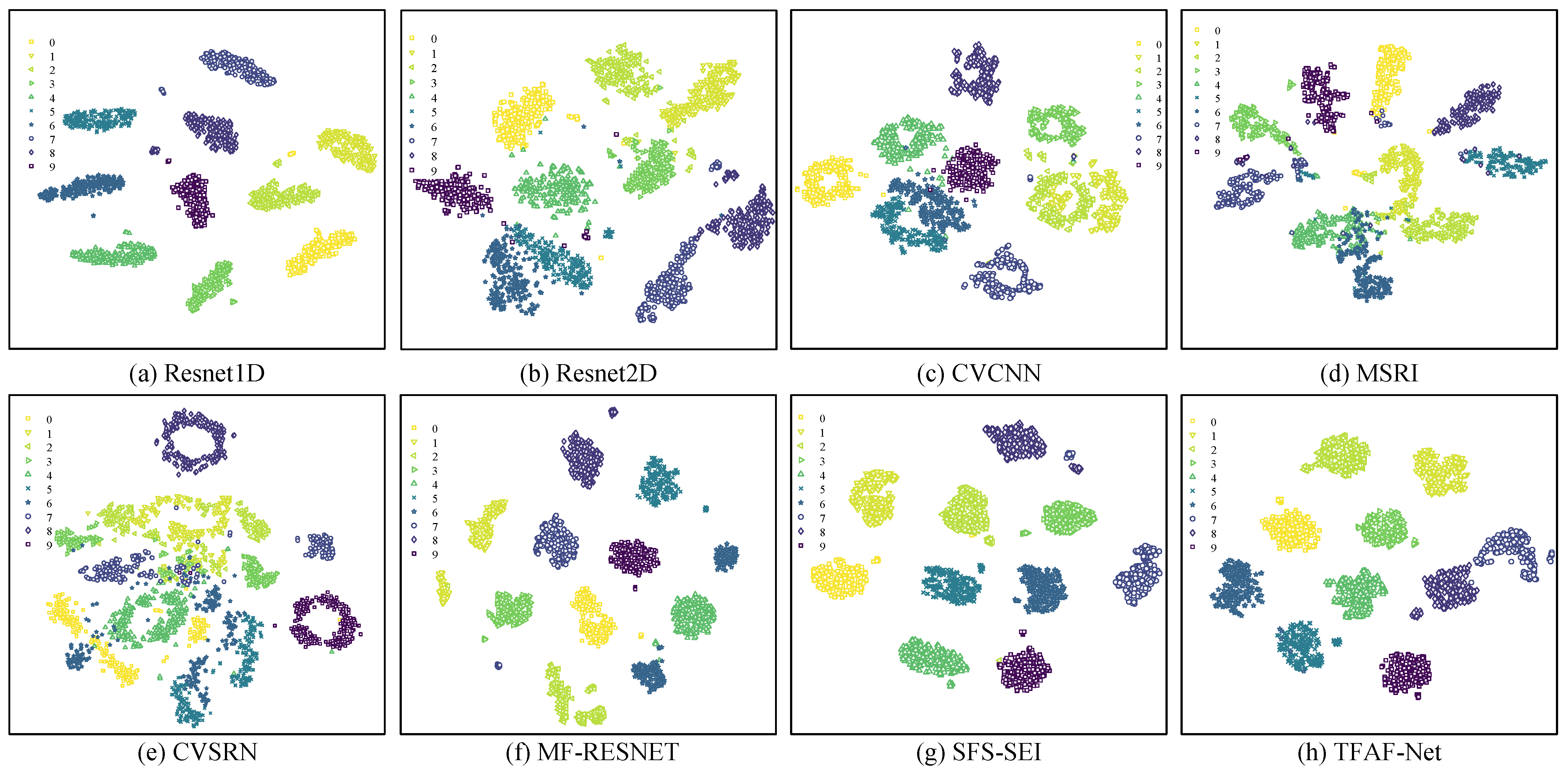
5.3. Few-Shot Signal Classification Compared with the Other Methods
5.4. Ablation Studies
5.4.1. Ablation of Time-Frequency Fusion Module
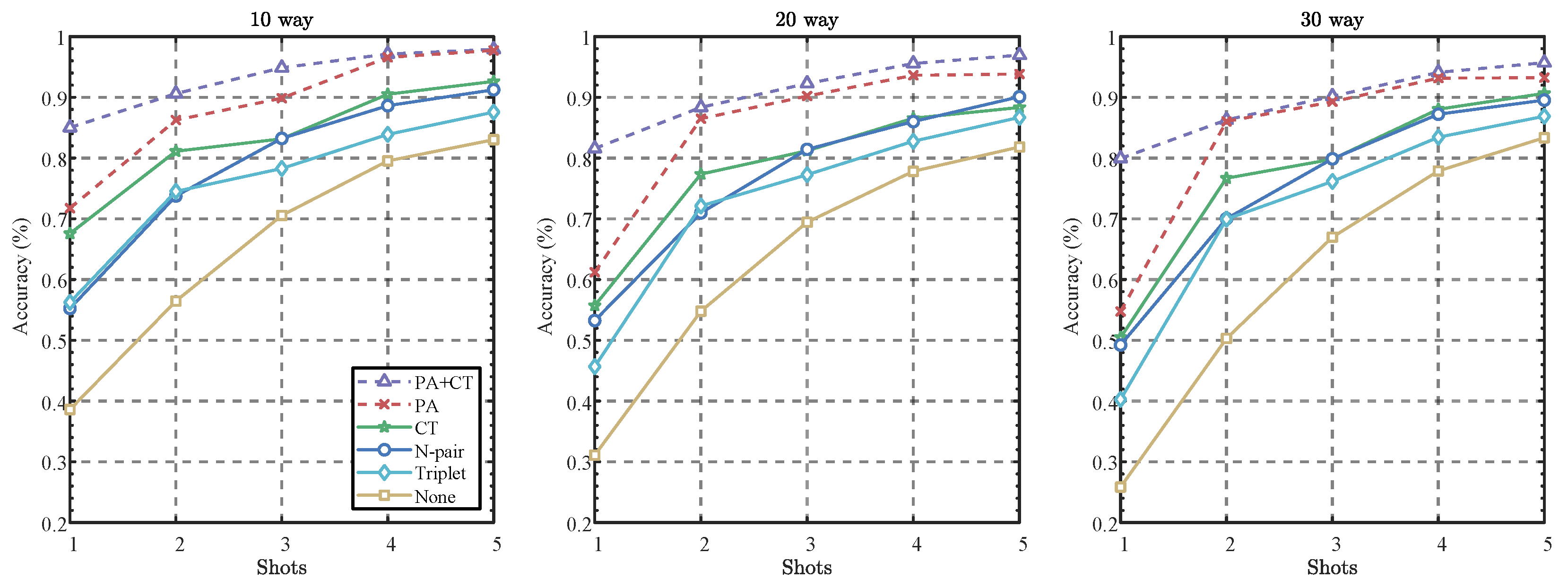
5.4.2. Evaluation of Loss Function Configurations: Ablation and Comparison
6. Conclusions
Author Contributions
Funding
Data Availability Statement
Conflicts of Interest
References
- Liu, P.; Guo, L.; Zhao, H.; Shang, P.; Chu, Z.; Lu, X. A Long Time Span-Specific Emitter Identification Method Based on Unsupervised Domain Adaptation. Remote Sens. 2023, 15, 5214. [Google Scholar] [CrossRef]
- Xu, Y.; Xu, C.; Feng, Y.; Bao, S. FSK Emitter Fingerprint Feature Extraction Method Based on Instantaneous Frequency. In Proceedings of the 2023 IEEE 23rd International Conference on Communication Technology (ICCT), Wuxi, China, 20–22 October 2023; pp. 397–402. [Google Scholar]
- Liu, Y.; Wang, J.; Li, J.; Niu, S.; Song, H. Machine Learning for the Detection and Identification of Internet of Things Devices: A Survey. IEEE Internet Things J. 2022, 9, 298–320. [Google Scholar] [CrossRef]
- Feng, Z.; Chen, S.; Ma, Y.; Gao, Y.; Yang, S. Learning Temporal–Spectral Feature Fusion Representation for Radio Signal Classification. IEEE Trans. Ind. Inform. 2024, 1–10. [Google Scholar] [CrossRef]
- Wiley, R. ELINT: The Interception and Analysis of Radar Signals; Artech: Norwood, MA, USA, 2006. [Google Scholar]
- Zhang, X.; Li, T. Specific Emitter Identification Based on Feature Diagram Superposition. In Proceedings of the 2022 7th International Conference on Integrated Circuits and Microsystems (ICICM), Xi’an, China, 28–31 October 2022; pp. 703–707. [Google Scholar]
- Jing, Z.; Li, P.; Wu, B.; Yan, E.; Chen, Y.; Gao, Y. Attention-Enhanced Dual-Branch Residual Network with Adaptive L-Softmax Loss for Specific Emitter Identification under Low-Signal-to-Noise Ratio Conditions. Remote Sens. 2024, 16, 1332. [Google Scholar] [CrossRef]
- Su, J.; Liu, H.; Yang, L. Specific Emitter Identification Based on CNN via Variational Mode Decomposition and Bimodal Feature Fusion. In Proceedings of the 2023 IEEE 3rd International Conference on Power, Electronics and Computer Applications (ICPECA), Shenyang, China, 29–31 January 2023; pp. 539–543. [Google Scholar]
- Wu, T.; Zhang, Y.; Ben, C.; Peng, Y.; Liu, P.; Gui, G. Specific Emitter Identification Based on Multi-Scale Attention Feature Fusion Network. In Proceedings of the 2023 IEEE 23rd International Conference on Communication Technology (ICCT), Wuxi, China, 20–22 October 2023; pp. 1390–1394. [Google Scholar]
- Wang, Y.; Gui, G.; Gacanin, H.; Ohtsuki, T.; Dobre, O.A.; Poor, H.V. An Efficient Specific Emitter Identification Method Based onComplex-Valued Neural Networks and Network Compression. IEEE J. Sel. Areas Commun. 2021, 39, 2305–2317. [Google Scholar] [CrossRef]
- Zhu, M.; Feng, Z.; Zhou, X. A novel data-driven specific emitter identification feature based on machine cognition. Electronics 2020, 9, 1308. [Google Scholar] [CrossRef]
- Woo, S.; Park, J.; Lee, J.Y.; Kweon, I.S. CBAM: Convolutional Block Attention Module. In Proceedings of the Computer Vision—ECCV 2018, Munich, Germany, 8–14 September 2018; Ferrari, V., Hebert, M., Sminchisescu, C., Weiss, Y., Eds.; Springer: Cham, Switzerland, 2018; pp. 3–19. [Google Scholar]
- Man, P.; Ding, C.; Ren, W.; Xu, G. A Specific Emitter Identification Algorithm under Zero Sample Condition Based on Metric Learning. Remote Sens. 2021, 13, 4919. [Google Scholar] [CrossRef]
- Huang, J.; Li, X.; Wu, B.; Wu, X.; Li, P. Few-Shot Radar Emitter Signal Recognition Based on Attention-Balanced Prototypical Network. Remote Sens. 2022, 14, 6101. [Google Scholar] [CrossRef]
- Kim, S.; Kim, D.; Cho, M.; Kwak, S. Proxy Anchor Loss for Deep Metric Learning. In Proceedings of the 2020 IEEE/CVF Conference on Computer Vision and Pattern Recognition (CVPR), Seattle, WA, USA, 13–19 June 2020; pp. 3235–3244. [Google Scholar]
- Wen, Y.; Zhang, K.; Li, Z.; Qiao, Y. A Discriminative Feature Learning Approach for Deep Face Recognition. In Proceedings of the Computer Vision—ECCV 2016, Amsterdam, The Netherlands, 11–14 October 2016; Leibe, B., Matas, J., Sebe, N., Welling, M., Eds.; Springer: Cham, Switzerland, 2016. [Google Scholar]
- Zhao, Y.; Yang, R.; Wu, L.; He, S.; Niu, J.; Zhao, L. Specific Emitter Identification Using Regression Analysis between Individual Features and Physical Parameters. In Proceedings of the 2022 6th International Conference on Imaging, Signal Processing and Communications (ICISPC), Kumamoto, Japan, 22–24 July 2022; pp. 48–52. [Google Scholar]
- Pan, Y.; Yang, S.; Peng, H.; Li, T.; Wang, W. Specific emitter identification based on deep residual networks. IEEE Access 2019, 7, 54425–54434. [Google Scholar] [CrossRef]
- Zhao, Y.; Wang, X.; Lin, Z.; Huang, Z. Multi-Classifier Fusion for Open-Set Specific Emitter Identification. Remote Sens. 2022, 14, 2226. [Google Scholar] [CrossRef]
- Zhang, X.; Wang, Y.; Zhang, Y.; Lin, Y.; Gui, G.; Tomoaki, O.; Sari, H. Data Augmentation Aided Few-Shot Learning for Specific Emitter Identification. In Proceedings of the 2022 IEEE 96th Vehicular Technology Conference (VTC2022-Fall), London, UK, 26–29 September 2022; pp. 1–5. [Google Scholar]
- Yao, Z.; Fu, X.; Guo, L.; Wang, Y.; Lin, Y.; Shi, S.; Gui, G. Few-Shot Specific Emitter Identification Using Asymmetric Masked Auto-Encoder. IEEE Commun. Lett. 2023, 27, 2657–2661. [Google Scholar] [CrossRef]
- Wu, Y.; Sun, Z.; Yue, G. Siamese Network-based Open Set Identification of Communications Emitters with Comprehensive Features. In Proceedings of the 2021 6th International Conference on Communication, Image and Signal Processing (CCISP), Chengdu, China, 19–21 November 2021; pp. 408–412. [Google Scholar]
- Wang, C.; Fu, X.; Wang, Y.; Gui, G.; Gacanin, H.; Sari, H.; Adachi, F. Interpolative Metric Learning for Few-Shot Specific Emitter Identification. IEEE Trans. Veh. Technol. 2023, 72, 16851–16855. [Google Scholar] [CrossRef]
- Yang, N.; Zhang, B.; Ding, G.; Wei, Y.; Wei, G.; Wang, J.; Guo, D. Specific Emitter Identification with Limited Samples: A Model-Agnostic Meta-Learning Approach. IEEE Commun. Lett. 2022, 26, 345–349. [Google Scholar] [CrossRef]
- Sankhe, K.; Belgiovine, M.; Zhou, F.; Riyaz, S.; Ioannidis, S.; Chowdhury, K. ORACLE: Optimized Radio clAssification through Convolutional neuraL nEtworks. In Proceedings of the IEEE INFOCOM 2019—IEEE Conference on Computer Communications, Paris, France, 29 April–2 May 2019; pp. 370–378. [Google Scholar]
- Liu, M.; Chai, Y.; Li, M.; Wang, J.; Zhao, N. Transfer Learning-Based Specific Emitter Identification for ADS-B over Satellite System. Remote Sens. 2024, 16, 2068. [Google Scholar] [CrossRef]
- He, K.; Zhang, X.; Ren, S.; Sun, J. Deep Residual Learning for Image Recognition. In Proceedings of the 2016 IEEE Conference on Computer Vision and Pattern Recognition (CVPR), Las Vegas, NV, USA, 27–30 June 2016; pp. 770–778. [Google Scholar]
- Zhimian, Z.; Haipeng, W.; Xu, F.; Jin, Y.-Q. Complex-Valued Convolutional Neural Network and Its Application in Polarimetric SAR Image Classification. IEEE Trans. Geosci. Remote Sens. 2017, 55, 7177–7188. [Google Scholar]
- Qian, Y.; Qi, J.; Kuai, X.; Han, G.; Sun, H.; Hong, S. Specific Emitter Identification Based on Multi-Level Sparse Representation in Automatic Identification System. IEEE Trans. Inf. Forensics Secur. 2021, 16, 2872–2884. [Google Scholar] [CrossRef]
- Han, G.; Xu, Z.; Zhu, H.; Ge, Y.; Peng, J. A Two-Stage Model Based on a Complex-Valued Separate Residual Network for Cross-Domain IIoT Devices Identification. IEEE Trans. Ind. Inform. 2024, 20, 2589–2599. [Google Scholar] [CrossRef]
- Ying, W.; Deng, P.; Hong, S. Channel Attention Mechanism-based Multi-Feature Fusion Network for Specific Emitter Identification. In Proceedings of the 2022 IEEE 4th International Conference on Civil Aviation Safety and Information Technology (ICCASIT), Dali, China, 12–14 October 2022; pp. 1325–1328. [Google Scholar]
- Tao, M.; Fu, X.; Lin, Y.; Wang, Y.; Yao, Z.; Shi, S.; Gui, G. Resource-Constrained Specific Emitter Identification Using End-to-End Sparse Feature Selection. In Proceedings of the GLOBECOM 2023—2023 IEEE Global Communications Conference, Kuala Lumpur, Malaysia, 4–8 December 2023; pp. 6067–6072. [Google Scholar]
- van der Maaten, L.; Hinton, G. Visualizing Data using t-SNE. J. Mach. Learn. Res. 2008, 9, 2579–2605. [Google Scholar]
- Sohn, K. Improved deep metric learning with multi-class n-pair loss objective. Adv. Neural Inf. Process. Syst. 2016, 29, 1857–1865. [Google Scholar]
- Hoffer, E.; Ailon, N. Deep metric learning using triplet network. In Proceedings of the Similarity-Based Pattern Recognition: Third International Workshop, SIMBAD 2015, Copenhagen, Denmark, 12–14 October 2015; Springer: Cham, Switzerland, 2015; pp. 84–92. [Google Scholar]

| Module | Layer Structure | Output Size | Parameters |
|---|---|---|---|
| Encoder | BatchNorm2D + CBAM Module | (B, 3, 193, 128) | 6 + 110 |
| Conv2D(64, 3 × 3, s = 2) + ReLU + BatchNorm2D | (B, 64, 97, 64) | 1792 + 128 | |
| MaxPool2D(2 × 2, s = 2) | (B, 64, 48, 32) | 0 | |
| Conv2D(128, 3 × 3, s = 2) + ReLU + BatchNorm2D | (B, 128, 24, 16) | 73,856 + 256 | |
| MaxPool2D(2 × 2, s = 2) | (B, 128, 12, 8) | 0 | |
| Conv2D(256, 3 × 3, s = 1) + ReLU + BatchNorm2D | (B, 256, 12, 8) | 295,168 + 512 | |
| MaxPool2D(2 × 2, s = 2) | (B, 256, 6, 4) | 0 | |
| Conv2D(512, 3 × 3, s = 1) + ReLU + BatchNorm2D | (B, 512, 6, 4) | 1,180,160 + 1024 | |
| AdaptiveAvgPool2D(2, 1) | (B, 512, 2, 1) | 0 | |
| Flatten + Feature Transformation(1024) | (B, 1024) | 2048 | |
| Classifier | Linear(1024, 512) + ReLU | (B, 512) | 524,800 |
| Linear(512, C) | (B, C) |
| Parameters for Simulation | Pre-Training | Fine-Tuning |
|---|---|---|
| Sample Dimensions | 2 × 3000 | 2 × 3000 |
| Categories in | 120 | 10, 20, 30 |
| Categories in | 10 | 5, 6 |
| Samples per Category in | 200∼600 | 1, 5, 10, 20, 30 |
| Samples per Category in | 4200 | 1, 5, 10, 20, 30 |
| Simulation Parameters | Pre-Training | Fine-Tuning |
|---|---|---|
| Maximum epochs | 300 | 100 |
| Init learning rate | 0.01 | 0.01∼0.0001 |
| Learning rate scheduler | CosineAnnealingWarmRestarts | Constant |
| Early stop epochs | 60 | 40 |
| Batch size | 64 | Experimental way |
| Loss balance parameters | 0.1, 0.01 | 0.1, 0.001 |
Disclaimer/Publisher’s Note: The statements, opinions and data contained in all publications are solely those of the individual author(s) and contributor(s) and not of MDPI and/or the editor(s). MDPI and/or the editor(s) disclaim responsibility for any injury to people or property resulting from any ideas, methods, instructions or products referred to in the content. |
© 2024 by the authors. Licensee MDPI, Basel, Switzerland. This article is an open access article distributed under the terms and conditions of the Creative Commons Attribution (CC BY) license (https://creativecommons.org/licenses/by/4.0/).
Share and Cite
Mu, S.; Zu, Y.; Chen, S.; Yang, S.; Feng, Z.; Zhang, J. Few-Shot Metric Learning with Time-Frequency Fusion for Specific Emitter Identification. Remote Sens. 2024, 16, 4635. https://doi.org/10.3390/rs16244635
Mu S, Zu Y, Chen S, Yang S, Feng Z, Zhang J. Few-Shot Metric Learning with Time-Frequency Fusion for Specific Emitter Identification. Remote Sensing. 2024; 16(24):4635. https://doi.org/10.3390/rs16244635
Chicago/Turabian StyleMu, Shiyuan, Yong Zu, Shuai Chen, Shuyuan Yang, Zhixi Feng, and Junyi Zhang. 2024. "Few-Shot Metric Learning with Time-Frequency Fusion for Specific Emitter Identification" Remote Sensing 16, no. 24: 4635. https://doi.org/10.3390/rs16244635
APA StyleMu, S., Zu, Y., Chen, S., Yang, S., Feng, Z., & Zhang, J. (2024). Few-Shot Metric Learning with Time-Frequency Fusion for Specific Emitter Identification. Remote Sensing, 16(24), 4635. https://doi.org/10.3390/rs16244635