Article

LULC-SegNet: Enhancing Land Use and Land Cover Semantic Segmentation with Denoising Diffusion Feature Fusion

by
Zongwen Shi
1,2,
Junfu Fan
1,3,*,
Yujie Du
1,
Yuke Zhou
3 and
Yi Zhang
4,5
1
School of Civil Engineering and Geomatics, Shandong University of Technology, Zibo 255000, China
2
School of Geographical Sciences, Nanjing University of Information Science and Technology, Nanjing 210044, China
3
State Key Laboratory of Resources and Environmental Information System, Institute of Geographic Sciences and Natural Resources Research, Chinese Academy of Sciences, Beijing 100101, China
4
College of Land Resources and Surveying Engineering, Shandong Agriculture and Engineering University, Zibo 255300, China
5
School of Geosciences and Info-Physics, Central South University, Changsha 410083, China
*
Author to whom correspondence should be addressed.
Remote Sens. 2024, 16(23), 4573; https://doi.org/10.3390/rs16234573
Submission received: 6 November 2024 / Revised: 4 December 2024 / Accepted: 4 December 2024 / Published: 6 December 2024

Abstract

:
Deep convolutional networks often encounter information bottlenecks when extracting land object features, resulting in critical geometric information loss, which impedes semantic segmentation capabilities in complex geospatial backgrounds. We developed LULC-SegNet, a semantic segmentation network for land use and land cover (LULC), which integrates features from the denoising diffusion probabilistic model (DDPM). This network enhances the clarity of the edge segmentation, detail resolution, and the visualization and accuracy of the contours by delving into the spatial details of the remote sensing images. The LULC-SegNet incorporates DDPM decoder features into the LULC segmentation task, utilizing machine learning clustering algorithms and spatial attention to extract continuous DDPM semantic features. The network addresses the potential loss of spatial details during feature extraction in convolutional neural network (CNN), and the integration of the DDPM features with the CNN feature extraction network improves the accuracy of the segmentation boundaries of the geographical features. Ablation and comparison experiments conducted on the Circum-Tarim Basin Region LULC Dataset demonstrate that the LULC-SegNet improved the LULC semantic segmentation. The LULC-SegNet excels in multiple key performance indicators compared to existing advanced semantic segmentation methods. Specifically, the network achieved remarkable scores of 80.25% in the mean intersection over union (MIOU) and 93.92% in the F1 score, surpassing current technologies. The LULC-SegNet demonstrated an IOU score of 73.67%, particularly in segmenting the small-sample river class. Our method adapts to the complex geophysical characteristics of remote sensing datasets, enhancing the performance of automatic semantic segmentation tasks for land use and land cover changes and making critical advancements.

1. Introduction

The automatic semantic segmentation of remote sensing images is a crucial research field in geographic information science with significant practical applications in remote sensing analysis. Advanced satellite remote sensing technology, we are now able to obtain high-resolution image data with rich features and spatial information. Remote sensing images have a broader spatial scale than other types of images, containing more details of land objects and a higher degree of complexity [1]. Remote sensing image classes are highly heterogeneous and complex, which often leads to challenges such as low accuracy, blurred boundaries, and imbalanced samples in the segmentation process [2,3]. These issues not only increase the difficulty of automatic semantic segmentation tasks but also indirectly affect the accuracy and generalization ability of the segmentation results [4,5,6]. Therefore, achieving remote sensing semantic segmentation requires more refined spatial information and texture details. Further, the diversity of land object features in morphology, texture, and scale increases the difficulty of recognition and classification, which imposes higher requirements for designing automatic remote sensing image segmentation algorithms [7,8]. These challenges become even more evident in large-scale land use and land cover (LULC) segmentation [9,10,11,12].
In deep learning for LULC segmentation, convolutional neural networks (CNNs) have become the mainstream framework. Variants of CNNs, such as the U-Net and Deeplab series, have improved the segmentation quality by capturing multi-scale features with spatial significance and their integration ability [13,14,15,16]. Networks with visual attention mechanisms further optimize the segmentation accuracy and enhance the ability to analyze complex image data by fusing spatial features and channel information in remote sensing data [16,17]. On the other hand, models with self-attention mechanisms, such as visual transformers (ViTs), capture global information and refine the complex interactions among pixels through matrix multiplication operations, providing a deep modeling method for the macro and micro features of images [18,19]. Swin Transformer effectively addresses the challenge of processing high-resolution images with its innovative moving window strategy, significantly improving feature extraction and content understanding for LULC segmentation tasks [20,21]. In remote sensing, for semantic segmentation tasks based on CNN and Transformer architectures, various deep feature extraction networks are required to perform visual feature extraction. However, as feature extraction networks deepen, many important shallow features are often lost, causing information bottlenecks [22]. In remote sensing semantic segmentation, information bottlenecks often lose the delicate spatial information and textural details of the input remote sensing images, increasing the heterogeneity and complexity of the visual features and limiting the accuracy of land object sample segmentation.
In the field of deep generative models, frameworks such as generative adversarial networks (GANs), variational autoencoders (VAEs), autoregressive models, and diffusion probabilistic models (DDPMs) have demonstrated outstanding potential in various applications, such as image synthesis, super-resolution, and image-to-image translation [23,24,25,26,27,28]. These generative models mainly focus on learning the pixel distribution of the images, and they excel at producing high-quality and realistic images and effectively abstracting and generalizing the basic data patterns, thereby capturing and learning the intrinsic semantics of images [29,30,31]. DDPM, which uses Markov chains and Langevin dynamics to model complex data distributions, has achieved remarkable results in high-resolution image generation and can generate realistic images and land features [23,24,32,33].
To address the problems of information bottlenecks in deep networks, especially the loss of spatial features in feature extraction networks, such as Transformer and CNN, we consider introducing the characteristics of DDPM. By integrating DDPM, we aim to alleviate the problem of spatial feature loss caused by using traditional Transformer and CNN models and, thus, improve the performance and efficiency of the model in handling image-related tasks. It enhances the model’s ability to capture spatial information and lays a solid foundation for improving the accuracy and detail reproduction of image processing tasks.
Considering the challenges in the current research, we propose a novel framework, LULC-SegNet (Figure 1), that integrates DDPM features specially designed for mining spatial details in remote sensing images and applying them to land use and land cover semantic segmentation. By utilizing the spatial detail features of remote sensing images, our framework significantly improves edge segmentation and detail resolution and enhances contour visualization and classification accuracy. The main innovations of this study include the following:
(1)
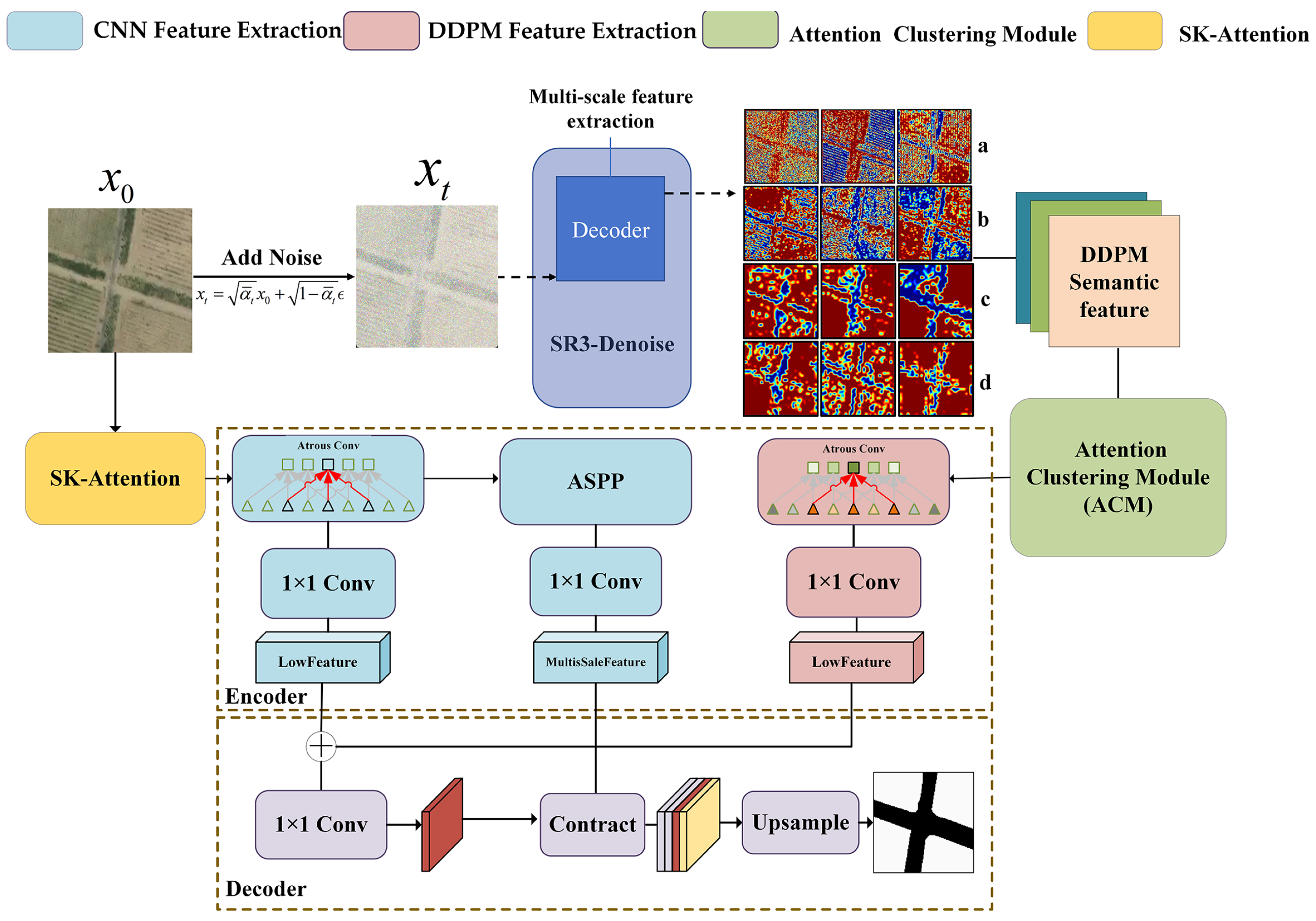
Introduction of the semantic features of the DDPM architecture into LULC segmentation and injecting semantic features into the CNN feature extraction network to address information;
(2)
Combining machine learning clustering algorithms and spatial attention mechanisms, and efficiently extracting the DDPM semantic features for LULC segmentation;
(3)
Verifying the significant effect of the DDPM on improving the performance of remote sensing image LULC segmentation through detailed ablation experiments and comparative studies.
In summary, our method adapts to the complex and diverse geophysical characteristics of remote sensing datasets, improves the performance of automatic semantic segmentation tasks for land use and land cover changes, and marks essential progress.

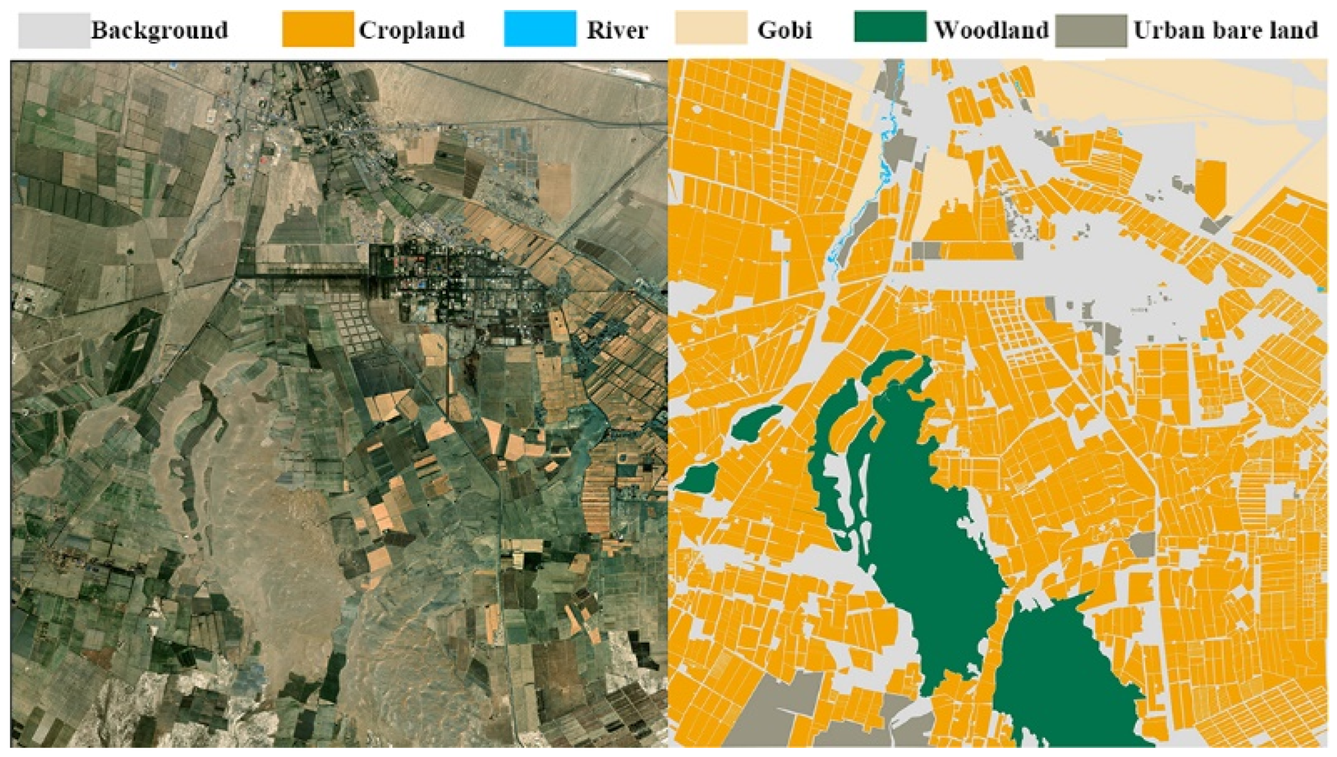
2. Study Area and Dataset

The primary study area is the Tarim Basin region in Xinjiang, China, which is far from the ocean, deep inland, and not easily reached by oceanic air currents, resulting in a distinct temperate continental climate [34,35]. The Tarim Basin is located in the southern part of Xinjiang and ring-shaped, with vast deserts in the interior and oases along the edges. The Circum-Tarim Basin region is thus rich in land-type samples. Its main sample categories include deserts, such as the Gobi, oases, and farmlands, water bodies, and many urban areas (Figure 2), with a substantial diversity of land cover categories.
For the LULC study in the Circum-Tarim Basin area, we constructed a dataset based on 0.59 m high-resolution remote sensing images from Mapbox sources. We accurately outlined the typical landform features by professional manual calibration methods. The dataset includes a total of six feature types, including desert, Gobi, farmland, water bodies, urban bare ground, and vegetation. However, the distribution of the number of pixels in each category is obviously imbalanced (Table 1), which exposes the unevenness of the sample categories. To train and validate the model, we divided the training set, validation set, and test set following a ratio of 6:2:2; these sets contained 11,232, 3742, and 3742 images, respectively, each with a resolution of 256 ×256 pixels. Notably, during the network training and validation phases, only the training and validation sets were included in the computation. In contrast, the test set remained independent and was not involved in the model training.

3. Materials and Methods

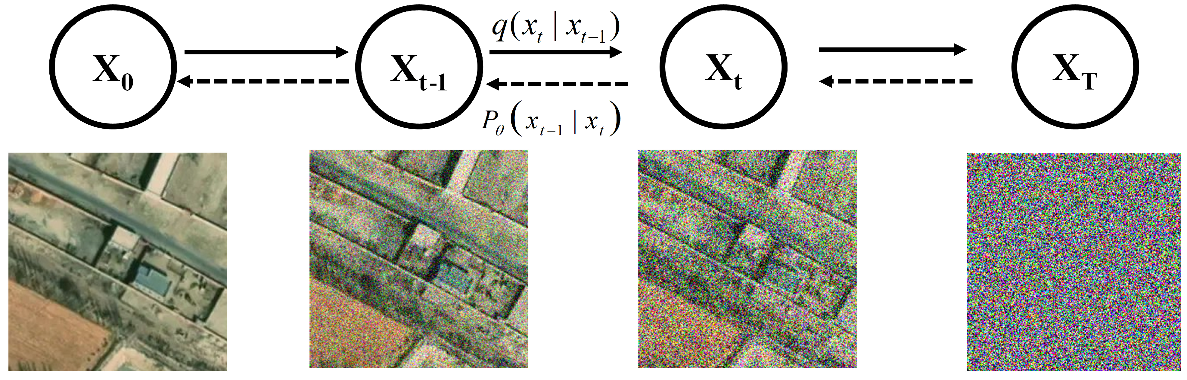
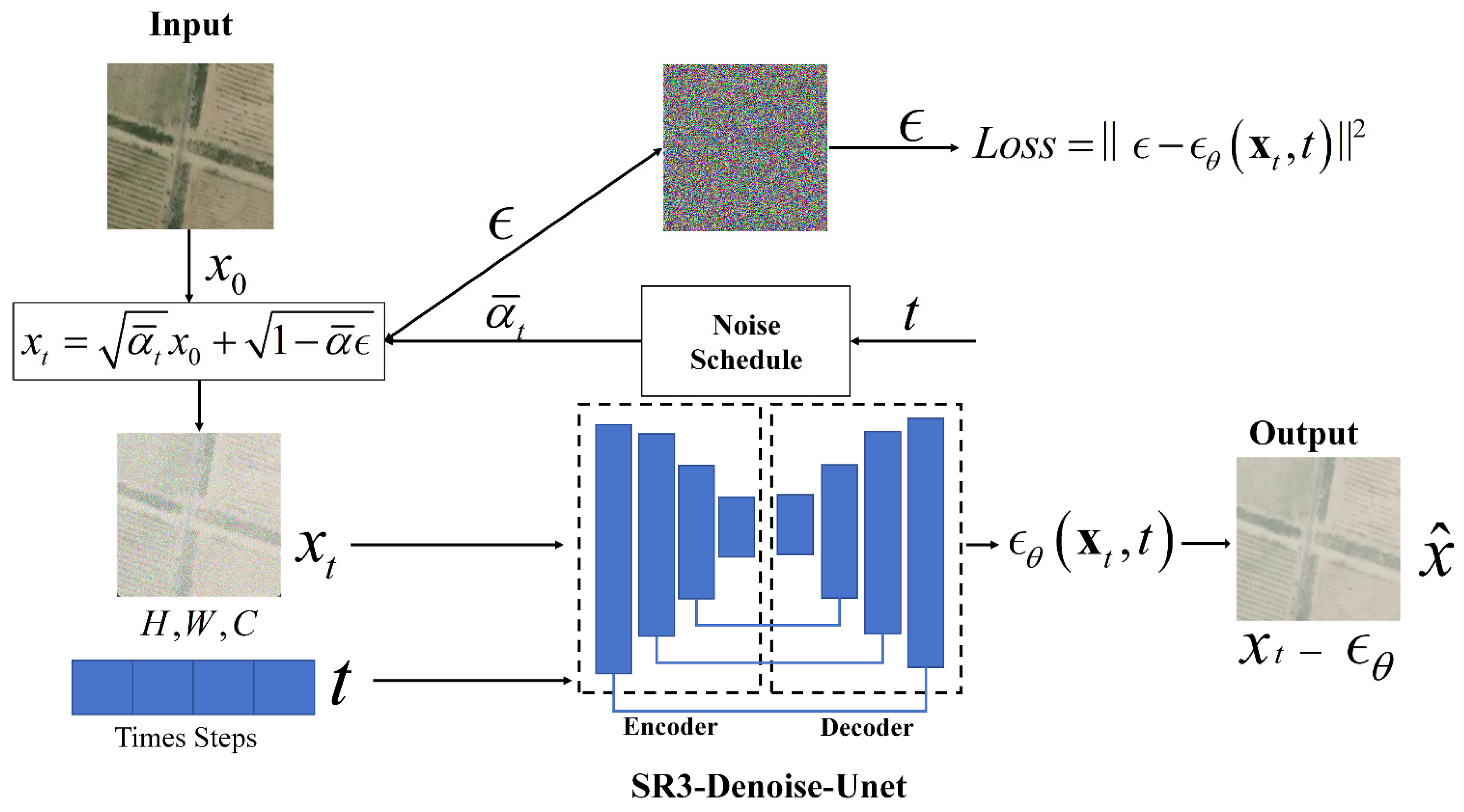
3.1. Denoise Diffusion Probabilistic Model

The Denoising Diffusion Probabilistic Model (DDPM) is a sophisticated generative framework that uses Markov chains and Langevin dynamics to replicate input data distribution through a finite sequence of steps [32,36]. This model initiates with a forward process where Gaussian noise is incrementally introduced to the data samples, morphing an original image,  X 0 , into a fully noise-enveloped specimen,   X t . In the reverse generation course, a neural network strips away the noise from the image in a sequential manner, successfully reconstructing a clean image that resonates with the input data’s distribution. Initiating from the noise-laden image,  X T , this reverse process methodically unravels through neural-network-powered denoising steps until it reclaims the original sample,  X 0 . Throughout this restoration journey, the DDPM showcases exceptional prowess in denoising and resynthesizing the data. The intricate principles and phases of the diffusion model are meticulously illustrated in Figure 3.
In the forward process  q ( x t | x t 1 ) , the image samples,  X , are incrementally corrupted by additive noise governed by a sequence of variance schedule,  β 1 , , β T , each associated with a discrete time step, t. The noise is  ϵ ~ N ( 0 , I ) , which obeys a Gaussian normal distribution, and  I  is the unit matrix. Specifically, it can be expressed as follows:
x t = 1 β t x t 1 + β t ϵ t ,
q ( x t | x t 1 ) = N ( x t | 1 β t x t 1 , β t I ) ,
Furthermore,  X t  can be obtained based on the sample  X 0 ,   as follows:  x t = α ¯ t x 0 + 1 α ¯ t ϵ , where  α ¯ t = k = 1 t α t     and   α t = 1 β t . Through the steps mentioned above, Gaussian noise is progressively applied on top of the image samples, gradually disturbing the image until a severely damaged image,  X t , is formed. This process is one of the core aspects of the diffusion model, which aims to create a series of diffusion data samples disturbed by noise.
The reverse process of the diffusion model is employed to reconstruct the original sample,  X 0 , by gradually removing the noise from the image sample,  X t , to which noise was added. Specifically, we start with the noise-containing sample  X t , estimate the noise using an iterative neural network, and compute the exact value of the noise using the noise estimation function  ϵ θ ( x t , t ) , where  θ  denotes the parameter set of the neural network model. Based on this, we can determine the denoised sample,  X t 1 , as follows:
x t 1 = 1 α t ( x t 1 α t 1 α ¯ t ϵ θ ( x t , t ) ) + σ t z ,
where  σ t z  is the predicted-noise-to-true-noise error,  Z ~ N ( 0 ,   1 ) . We, thus, obtain the inverse process,  p θ   ( x t 1   | x t ) ,  of the diffusion model as follows:
p θ   ( x t 1   | x t ) = N ( x t 1 ; μ θ ( x t , t ) , θ ( x t , t ) ) ,
μ θ ( x t , t ) = 1 α t x t 1 α t 1 α ¯ t α t ϵ θ ( x t , t ) ,
the U-Net model is typically used to refine the noise output iteratively [32,33,38]. Here,  x 0  represents the original sample;  x t  represents the sample to which the noise is added;  t   is the number of time steps, which represents the variance schedule corresponding to time stept; and  ϵ ^ θ  is the predicted value of the noise, which yields  x t 1 = x t ϵ ^ θ . Subsequently, the noise is estimated continuously and iteratively until  x ^ 0  is obtained.
L o s s = ϵ ϵ 0 ( α ¯ t x t 1 + 1 α ¯ t ϵ , t ) 2 .

3.2. Unsupervised Image Generation Based on DDPM

The diffusion model’s inverse-generated noise decoder can efficiently capture semantic information. The features extracted from the intermediate layer blocks of the generative model decoder are highly discriminative for image semantic segmentation, and these intermediate-generated feature representations can also correspond to pixel points with the same semantics [33,39,40]. We use the DDPM-based SR3 (Super-Resolution via Repeated Refinement) image generation model for unsupervised image synthesis. The SR3 generation process begins with pure Gaussian noise, and the noise output is iteratively optimized via a U-Net model trained on different noise levels. SR3 demonstrates a robust performance in super resolution tasks at different magnifications for scenes such as faces and natural images. It can generate unsupervised unconditional high-resolution images from image-to-image conversion [24,33]. Figure 4 represents the process of unsupervised image generation for SR3.

3.3. LULC Semantic Segmentation Network

We propose the LULC-SegNet which integrates the intermediate feature semantics and the sample feature fusion of the diffusion model SR3—achieved by adding t-step noise to the original sample,  X 0 , to generate a noisy version,  X t , feeding  X t  and  t  into the SR3-Denoise-UNet diffusion model for processing, obtaining the feature representation of the image by the SR3 Decoder. In Figure 1, the image’s semantic feature is shown. Figure 1 (a) and (b) illustrate the edge and gradient features of the LULC image, while (c) and (d) illustrate the abstract semantic features of the LULC image. Moreover, different feature representations can be obtained by varying  t  to adjust the noise level as follows:
f SR 3 - Decoder ( x , s t e p s ) = { F 1 t 0 , F 2 t 0 , F 3 t 0 , F 4 t 0 F 1 t 1 , F 2 t 1 , F 3 t 1 , F 4 t 1 F 1 t 2 , F 2 t 2 , F 3 t 2 , F 4 t 1 } ,
F i = C a t ( [ F i t 0 , F i t 1 , F i t 2 ] , dim = 1 ) ,   i { 1 , 2 , 3 , 4 } ,
where x is the input image sample, and steps are the noise steps. The sampling steps significantly impact semantic features, as appropriate steps can effectively capture semantic information. Therefore, we set steps = [50, 100, 400] [37]. Fi represents the geometric features generated by the multi-scale SR3-Decoder, Fi dimensions are as follows:
[ F 1 F 2 F 3 F 4 ] = [ ( H ,   W ,   64 ) ( H 2 , H 2 , 128 ) ( H 4 , H 4 , 256 ) ( H 8 , H 8 , 512 ) ] .
The LULC-SegNet consists of an encoder and a decoder, where the encoder contains an attention module, atrous convolution, atrous spatial pyramid pooling (ASPP), and the attention and clustering module (ACM) from the DDPM. We elaborate on the principles and functions of each module, highlighting our performance.
Attention Module: Remote sensing images usually contain rich spatial information and complex surface features, so we adopt selective kernel (SK) attention to capture these information features. SK-Attention dynamically selects the size of the convolution kernel to adapt to the different scales of high-resolution remote sensing images, which helps the network learn local features and adjust its attention according to global information [41]. The SK-Attention machine demonstrates remarkable advantages in multi-scale feature fusion [42]. Under comparable computational complexity, SK-Attention can effectively capture more intricate feature relationships, thereby significantly improving model performance [43]. Specifically, the implementation method of SK-Attention is as follows:
S = GlobalAvgPool ( U ) , U = i = 1 M U i , Z = Linear ( S ) , A i = Linear i ( Z ) , Attention   Weights = Softmax ( [ A 1 , A 2 , , A M ] ) , V = i = 1 M ( Attention   Weights i U i ) ,
where  M  is the number of convolution branches,  U i  is the feature map output by the i-convolution branch,  S  is the description of the global feature pooling output,  Z  is the low-dimensional space representation after feature mapping, linear is the fully connected layer, attention weights are the normalized attention weights, and  V  is the final output feature map.
Atrous Convolution: Atrous convolution is an extended convolution kernel achieved by adjusting the atrous rate in the convolution kernel. The atrous rate defines the interval between the values in the convolution kernel, and the larger the atrous rate, the wider the receptive field. Atrous convolution can help the model capture a more extensive range of contextual information without reducing the resolution of the feature map. Therefore, we use atrous convolution to generate shallow features by performing feature extraction on the image and then pass the low feature into the ASPP module to generate multi-scale image semantic features. In the LULC-SegNet, atrous convolution is implemented as follows:
Output ( y , x ) = i , j Input ( y + i r , x + j r ) Kernel ( i , j ) ,
where  y  and  x  are the position coordinates in the output feature map, with  x   as the horizontal coordinate, and  y  as the vertical coordinate;  r   is the atrous rate; and i and j are the indices of the convolution kernel.
ASPP: Considering the richness of the sample features of remote sensing images, especially in terms of texture and color details, we adopt the spatial pyramid pooling mechanism to further mine the abstract texture and color detail features in remote sensing images [44]. This method enables us to capture the semantic deep features at different scales, combine these deep features with shallow features, and pass them to the decoder for processing. The implementation strategy of the ASPP reflects a deep understanding and effective extraction of the multi-scale semantic features from remote sensing images, optimizes the model’s ability to capture detailed information, and provides strong technical support for accurate remote sensing image analysis, as follows:
b i ( x ) = ReLU ( BN ( Conv k i , d i ( x ) ) ) , g ( x ) = Upsample ( ReLU ( BN ( Conv 1 × 1 ( GlobalAvgPool ( x ) ) ) ) ) , Output ( x ) = Conv 1 × 1 ( Concat ( b 1 , b 2 , b 3 , b 4 , g ) ) ,
where   b i   denotes the feature generated by the i-th branch,  k i  denotes the size of the convolution kernel of the i-th branch,  d i  denotes the dilation rate of the i-th branch, g denotes the global feature branch, ReLU denotes the activation function, BN denotes batch normalization, Concat denotes concatenation operation, Upsample denotes upsampling to match the size of the original feature map, and a size (1,1) convolution kernel is used to unify the channels.
ACM in the DDPM: To address the issue of the original semantic features generated by the U-Net decoder from the diffusion model being abstract, dispersed, and containing a certain amount of independent semantic information that is irrelevant to the features to be segmented, we adopt the K-means clustering algorithm to aggregate the features [39]. Specifically, we divide the semantic sample data into K-clusters and assign the semantic features of each pixel from the diffusion model to the closest cluster. Moreover, we utilize the channel and spatial attention modules [41,45,46] to capture the more frequently occurring semantic information and combine it with the diffused semantic features obtained by the clustering algorithm to generate the final semantic information. This process aims to enhance the feature characteristics’ representational power and reduce irrelevant information’s impact on the network convergence.
To select the optimal number of K-clusters, for the clustering algorithm, we sample the segmentation dataset and use the gap statistic [47] to determine the best K. In our study area, we sample the LULC segmentation set. The sampled data are input into the pre-trained SR3 image generation model to produce the DDPM features. Then, cluster analysis and calculation of the gap statistic are performed on K. This process ensures that we can select the appropriate K-clusters based on the characteristics of the data themselves when dealing with remote sensing image segmentation tasks, thereby optimizing the segmentation performance and improving the overall efficiency of the model. The main goal of the gap statistic is to determine the optimal number of clusters in the cluster analysis. The gap statistic is calculated as follows:
W k = r = 1 k x C r d ( x , μ r ) 2 , G a p ( n , k ) = E n * [ log ( W k ) ] log ( W k ) ,
where  k  is the number of clusters,  C r  is the r-th cluster,  x   is a sample point,  d  is the distance from the sample point x to the cluster C,  W k  is the cluster dispersion, and  E  is the expectation.
We used the gap statistic to comprehensively evaluate and select  k = argmax k Gap ( n , k )  as the optimal number of clusters. In Figure 5, we analyzed the gap statistic values of the sampled data under different K-clusters. We found that the gap statistic reached the maximum value when the number of K-clusters = 5. We decided to use  k = 5  in the clustering algorithm experiment. The subsequent ablation experiments further verified the effectiveness of using the gap statistic to determine the number of clusters. In addition, we performed SK-Attention calculations on the DDPM features processed by the clustering algorithm to generate coherent DDPM semantic features. Specifically, the calculation process of the ACM is as follows:
C l u s t e r i = K - Means ( F i , k ) ,     i { 1 , 2 , 3 , 4 } , A t t e n i o n i = SK - Attention ( C l u s t e r i ) ,     i { 1 , 2 , 3 , 4 } , A t t e n i o n = Cat ( A t t e n i o n i ) ,   i { 1 , 2 , 3 , 4 } , Output = Conv 1 × 1 ( A t t e n i o n ) .
Encoder: The encoder’s feature extraction based on remote sensing image LULC primarily involves extracting land abstract texture color details and edge shape shallow features. Extracting the abstract texture color details captures the land cover type and texture feature information to enhance the classification and recognition of pixels. Extracting the edge shape shallow features helps to capture the land boundary and shape change information to enhance LULC segmentation and boundary detection in the image. Specifically, we use the atrous convolution to expand the perceptual field to extract the semantic features of remote sensing image sample  X  at a spatial scale and the feature edge shape features of the semantic feature generated by the diffusion decoder. Then, we splice sample  X  after the cavity convolution layer with the shallow features of the semantic feature generated by the diffusion decoder to fuse the semantic features and the edge shape features. Meanwhile, considering that the remote sensing image sample,  X ,  has rich texture color features, we adopt the spatial pyramid pooling mechanism ASPP to further extract the abstract texture color detail features in the remote sensing image to obtain its multi-scale semantic deep features and pass them and the shallow features into the decoder. The decoder performs channel compression of the shallow features with the deep features, followed by upsampling for the LULC segmentation.
Decoder: The decoder first integrates the semantic features obtained from the DDPM decoder with the low-level features extracted from the original remote sensing image. After adjusting the channel number of the low-level features through a convolutional layer, it is consistent with the high-level features. Subsequently, these low-level features with adjusted channel numbers are combined with the multi-scale features obtained by the ASPP module. Finally, the pixel-wise classification task is completed by upsampling to the original image size.

3.4. Hybridization Loss Function

To address the training sample imbalance in the LULC segmentation dataset, we employ a multiple loss function weighted average approach as a loss. Focal loss [48] addresses category imbalance by varying the standard cross-entropy loss function, thus reducing the loss weights assigned to correctly categorized samples. Focus loss can focus training on a sparse set of complex examples and mitigate the impact of many simple negative samples on the network during training. This approach uses two predefined hyperparameters,  α t  and  γ , where  α t  is used to reduce the loss contribution from simple examples and to extend the influence of the examples, and  γ  is used to address the category imbalance, as follows:
F o c a l L o s s ( p t ) = α t ( 1 p t ) γ log ( p t ) .
Dice loss [49] is an ordinary loss function used for image segmentation tasks to measure the similarity between the model’s predicted results and the true segmentation mask. It is based on the concept of the F1 score, which combines the precision and recall of the classification model to comprehensively evaluate the model’s performance. The Dice loss is calculated by comparing the proportion of overlapping regions between the predicted segmentation results and the true segmentation mask to obtain the F1 score and then subtracting the F1 score from 1 to obtain the Dice loss. The value of the Dice loss is in the range of 0 to 1. A value closer to 0 indicates that the model’s prediction is less similar to the real result, while a value closer to 1 indicates that the two results are more similar. The Dice loss has some advantages over the traditional cross-entropy loss function in handling sample imbalance. While the traditional cross-entropy loss may cause the model to be biased toward predicting a more significant number of categories, the Dice loss can consider each category in a more balanced way, preventing the model from being overly biased toward the majority categories and, thus, ignoring the minority categories. This allows the Dice loss to mitigate the bias problem of the model when handling sample imbalance and improving the segmentation accuracy for all categories. Additionally, the Dice loss utilizes overlapping regions for computation, allowing the model to pay more attention to the accuracy of edges when predicting segmentation boundaries. This improves the quality of the segmentation results, especially when handling targets with complex boundaries [50].
D i c e L o s s = 1 2 T P 2 T P + F N + F P .
The cross entropy loss function [51] works by logarithmically transforming the probability values output from the model, multiplying the result with the corresponding true labels and then performing a summation operation with negative values. By minimizing the cross-entropy loss, the model’s predictions can be made to better align with the distribution of the true labels. When the cross-entropy loss function is used for training, if the model classifies a sample correctly, the loss tends to zero; if the model misclassifies a sample, the cross-entropy loss tends to positive infinity. Therefore, minimizing the cross-entropy loss is equivalent to maximizing the probability of correct classification and minimizing the probability of misclassification, as follows:
C E L o s s ( p t ) = α t log ( p t ) .
Cross-entropy loss is usually more likely to converge to sharp minima with poor generalization performance; as a result, the model can effectively and quickly converge, but its generalizability cannot be easily improved [52]. Meanwhile, the Dice loss, while effective for mitigating the data imbalance problem, is not practical for quicker and better convergence of the model in highly imbalanced segmentation tasks, which leads to difficulties in model training [53]. Therefore, we use hybrid loss functions to train neural networks; by employing multiple hybrid loss functions, we can utilize the advantages of each loss function while effectively limiting their disadvantages [52,54], improving the convergence efficiency of the network [55], and alleviating the category imbalance problem in semantic segmentation [56]. We perform hyperparameter-weighted averaging of the focal loss, dice loss, and cross entropy loss to alleviate the category imbalance problem in the LULC segmentation networks, as follows:
M i x e d   L o s s = W 1 × F o c a l L o s s + W 2 × D i c e L o s s + W 3 × C E L o s s ,
where W1, W2, and W3 are the weight parameters for mixed loss. When the training sample classes are balanced, cross-entropy loss is widely regarded as an effective loss function for classification tasks due to its natural alignment with probability distributions [57], its efficacy in multi-class classification, its provision of stable and meaningful gradient information [58], and its outstanding performance on large-scale datasets [59]. In imbalanced samples, introducing Focal loss and Dice loss can mitigate the class imbalance issue; however, it significantly increases the difficulty of network training [49,60,61,62]. Therefore, assigning equal weights should be avoided when setting the weight parameters for a combined loss function. Increasing the weight of the cross-entropy loss is generally believed to effectively alleviate the training difficulties introduced by Dice loss and the parameter sensitivity drawbacks of the Focal loss [51,63,64].

3.5. Evaluation Metric

We choose three metrics, including pixel accuracy (PA), F1 score, and intersection over union (IOU), to validate the effectiveness of the proposed model. The higher the precision and recall, the more accurately the model detects changed pixels. The higher the F1 score and IOU, the better the model’s overall performance. The four metrics are calculated as follows:
P A = T P + T N T P + F P + T N + F N ,
P = T P T P + F P ,
R = T P T P + F N ,
F 1 = 2 P × R P + R ,
I O U = T P T P + F P + F N ,
where TP denotes the pixels that changed and are predicted to change by the model, TN denotes the pixels that did not change and are predicted to not change by the model, FP denotes the pixels that did not change but are predicted to change by the model, and FN denotes the pixels that changed but are predicted to not change by the model.

4. Result

In this section, we experimentally confirm the advantages of the DDPM-based characterization for the LULC segmentation problem. We first present the experimental details and parameter settings, then report the ablation study results of each module of the LULC-SegNet, and, finally, compare our method with the current state-of-the-art (SOTA) models to demonstrate the method’s effectiveness and theory.

4.1. Experimental Details

We trained our model on a server equipped with two NIVIDA RTX3090 GPUs (NIVIDA, Santa Clara, CA, USA). We used 20,000 unlabeled high-resolution remote sensing images of size 256 × 256 pixels from the Tarim Basin region to perform unsupervised training on the SR3 image diffusion generative model and obtain the pre-trained SR3 image generative model. In the training phase, to enhance the model’s generalization ability, we adopted various data augmentation techniques, including random resizing (80% to 120% randomized scaling), random horizontal flipping (75% horizontal flip chance), and random cropping (crop ratio [0.8, 1.0] and aspect ratios [3/4, 4/3]). We chose the AdamW optimizer (initial learning rate = 3.5 × 10⁻³, weight_decay = 1 × 10⁻², and eps = 1 × 10⁻⁸) and used the cosine annealing optimization scheduler (T_max = 25 and eta_min = 0). In the evaluation phase, we paid particular attention to maintaining the original aspect ratio of the remote sensing images and processed them by adjusting the short side of the image to the cropping size during training to ensure the accuracy of the evaluation. We did not use training tricks and only adjusted the loss function to cope with the class imbalance problem in the dataset. All models in the experiments used the same loss function weight settings ( W 1 W 2 , and  W 3  were 0.3, 0.3, and 0.4, respectively) to ensure the consistency of the experimental conditions. It is worth noting that all experimental results were obtained based on an independent test set that did not participate in the training process, thus ensuring the fairness and reliability of the results.

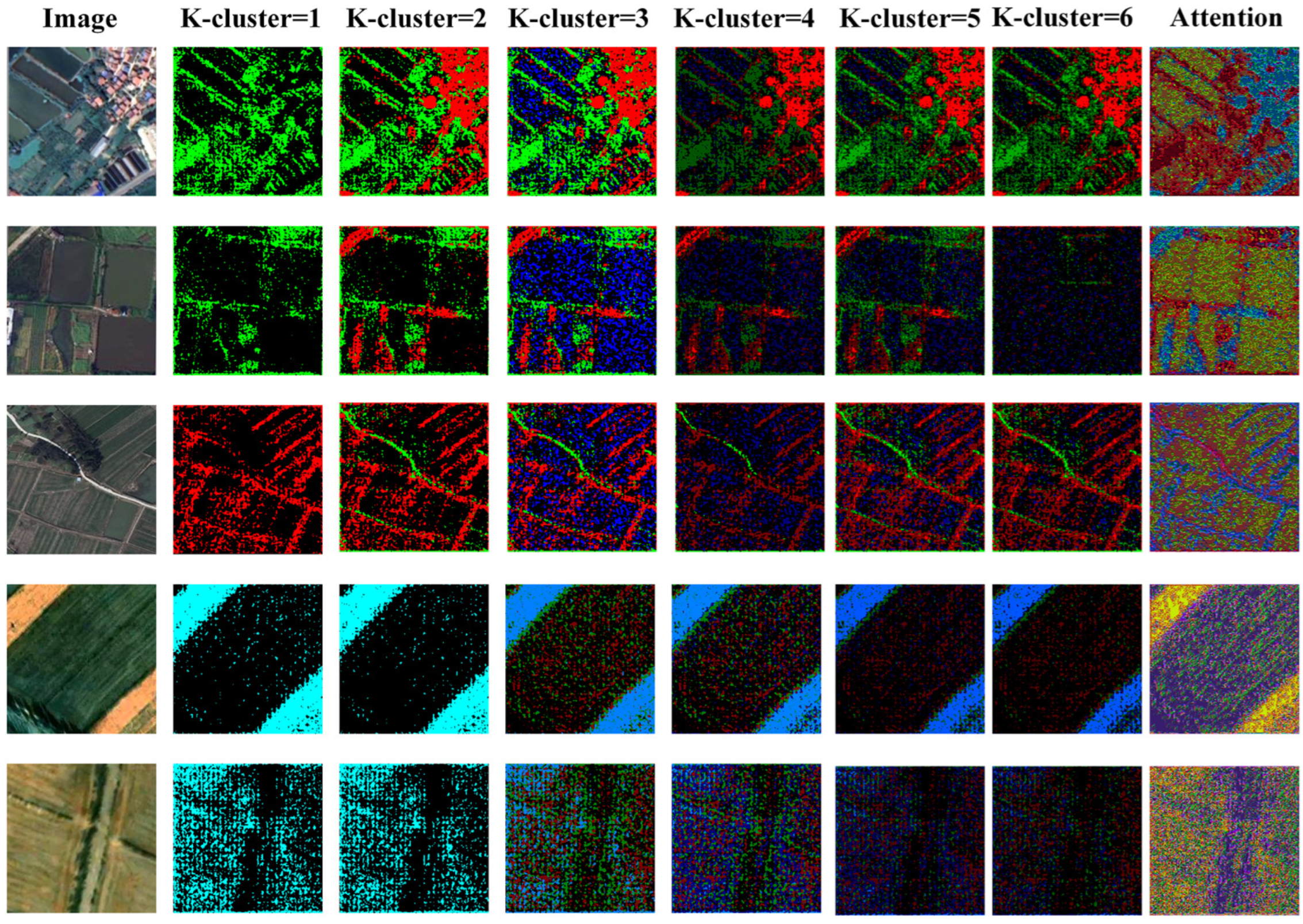
4.2. ACM in the DDPM Ablation Study

We investigated the impact of different K-clusters on the experimental results by adjusting the ACM while keeping the LULC-SegNet architecture intact. The specific experimental settings were as follows: 1. Remove the SK-Attention module, retain only the clustering operation on the DDPM features, and adjust the differen K-clusters to obtain quantitative experimental results. 2. Add the SK-Attention module and the clustering operation on the DDPM features and adjust different K-clusters to obtain quantitative experimental results. Table 2 shows the quantitative results of our ablation experiments.
The experimental results show that when K-cluster = 5, the model achieved an MIOU and F1 score consistent with the K-clusters determined by the gap statistic. Meanwhile, applying SK-Attention enhanced the model performance. We further visualized the aggregated features of the K-means clustering algorithm on the SR3 generative model decoder under different K-cluster settings (Figure 6) and found that a K-cluster = 5 can generate semantic features with the richest ground truth characteristics and the slightest noise (Figure 7). When K-cluster < 5, the generated semantic features fail to express the land features fully; when the K-cluster > 5, the diffuse semantic features contain information irrelevant to the segmentation target. Therefore, in the subsequent LULC segmentation network, we chose K-cluster = 5 to represent the diffuse semantic features of the original remote sensing image. The visualization results further show that after adding SK-Attention, the continuous feature contours and more abstract semantic details can be expressed more accurately, optimizing the model’s segmentation performance.

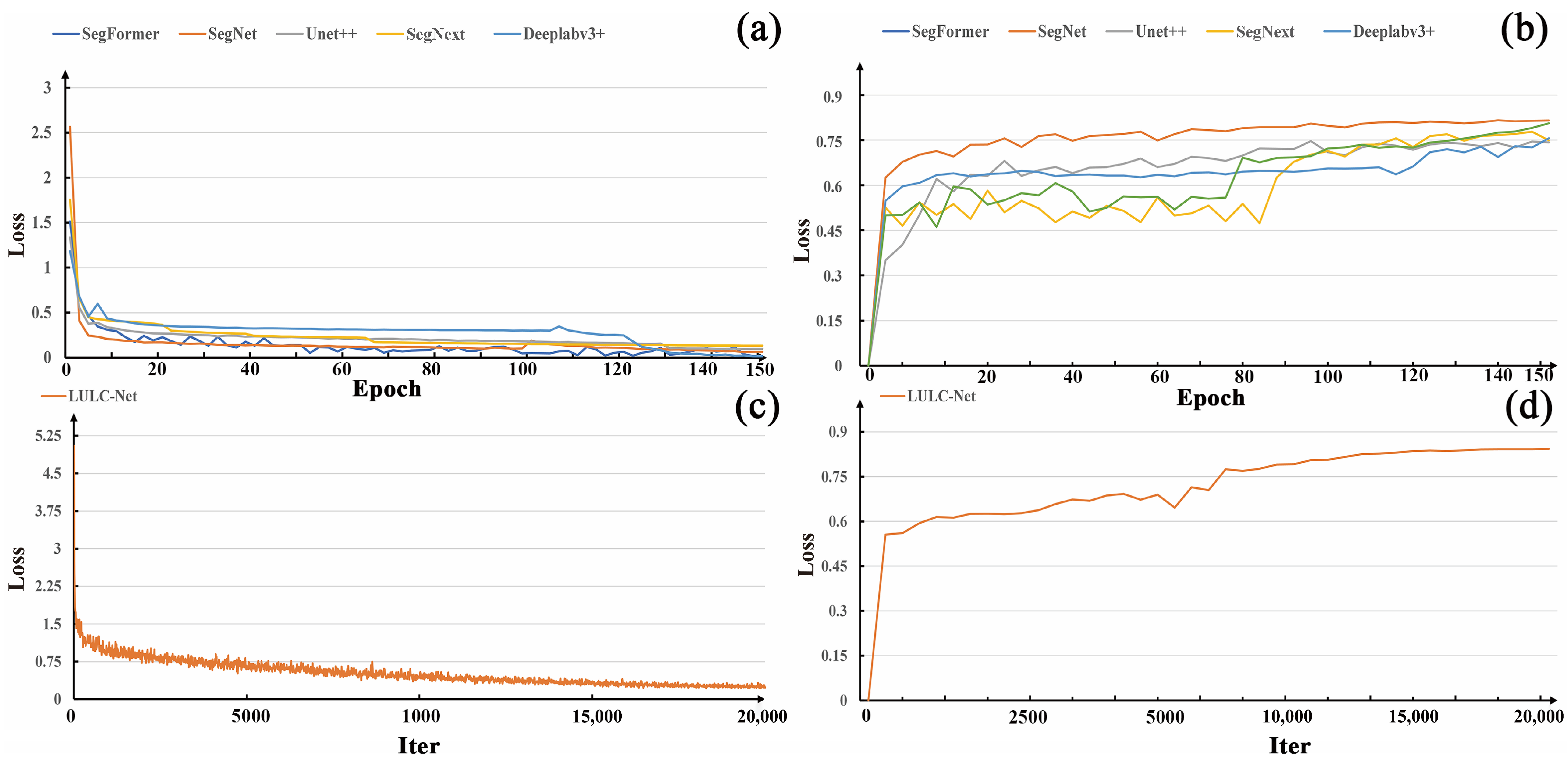
4.3. LULC Segmentation Network Ablation Study

This section describes the ablation experiments to demonstrate the improvement in the LULC segmentation performance by introducing the clustered DDPM features and applying the attention module in the LULC-SegNet. Table 3 shows the results of the ablation experiments. The results indicate that using only CNN feature extraction (ASPP and dilated convolution), the model shows an essential LULC segmentation performance, achieving a 72.65% MIOU, 90.25% OA, and 89.63% F1 score. After introducing the SK-Attention module, although the MIOU slightly decreased, the overall accuracy and F1 score increased, reaching 92.63% and 92.87%, respectively, which suggests that the attention mechanism can enhance the feature representation ability and improve the segmentation accuracy. When adding the DDPM ACM (K-cluster) after the CNN feature extraction, the model performance significantly improved, achieving a 79.25% MIOU, 92.22% OA, and 91.64% F1 score, which indicates that the DDPM features introduced by clustering had a significant positive impact on the LULC segmentation performance. Finally, the model achieved an optimal performance by combining the DDPM ACM (K-cluster) and the SK-Attention module, with 80.25%, 93.92%, and 92.92% scores in all evaluation metrics.

4.4. LULC Segmentation Network Quantitative Comparison Experimental Results

We compare the developed LULC segmentation algorithm with today’s leading semantic segmentation methods, which include SegNet, a deep convolutional codec architecture designed for image segmentation [65]; U-Net++, a network architecture that combines long-range and short-range connectivity [66]; DeepLabV3+, a codec architecture that employs null separable convolutional techniques for deeper semantic image segmentation [44]; SegNext employs a robust Vision Transformer architecture with a Multi-Scale Convolutional Attention Module (MSCA) to effectively capture semantic information across various scales, facilitating efficient semantic segmentation [67]; and SegFormer, a semantic segmentation model that utilizes a multihead self-attention mechanism [68], which combines a CNN architecture with a nonlocal attention (i.e., transformer) structure that is considered an SOTA network. In comparing the results of these methods, we set the training parameters of each network model equal to the settings in the original paper, ensuring fair and comparable results. During network training, we terminated training as soon as the loss of the training set and the mean intersection ratio (Miou) of the validation set exhibited stabilizing trends (see Figure 8), which ensured a thorough evaluation of the performance of each network model. This strategy allows the model to efficiently control the training process, optimize the network models after sufficient iterations, and perform optimally on the validation set.
Using the MIOU and F1 score as the evaluation criteria, our LULC-SegNet network outperforms the other network models in segmentation in all categories. The LULC-SegNet achieved obvious improvements in segmentation for the urban bare land, woodland, and cropland categories, reaching a high segmentation IOU of 59.14%, 93.26%, and 91.32%, respectively (see Table 4). Overall, the MIOU of the LULC-SegNet reached 80.25%, while the F1 score evaluation index, which combines precision and accuracy, also reached 93.92%. Through the permutation testing, we demonstrate that the LULC-SegNet exhibits advantages over other networks, particularly in effectively enhancing the segmentation performance under conditions of class imbalance. Additionally, the inference efficiency of the LULC-SegNet surpassed that of the segmentation networks based purely on the Transformer architectures.

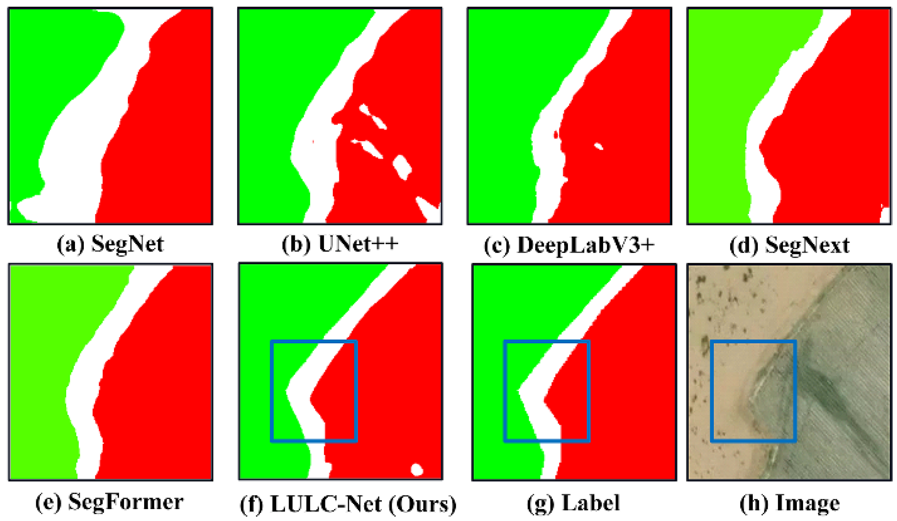
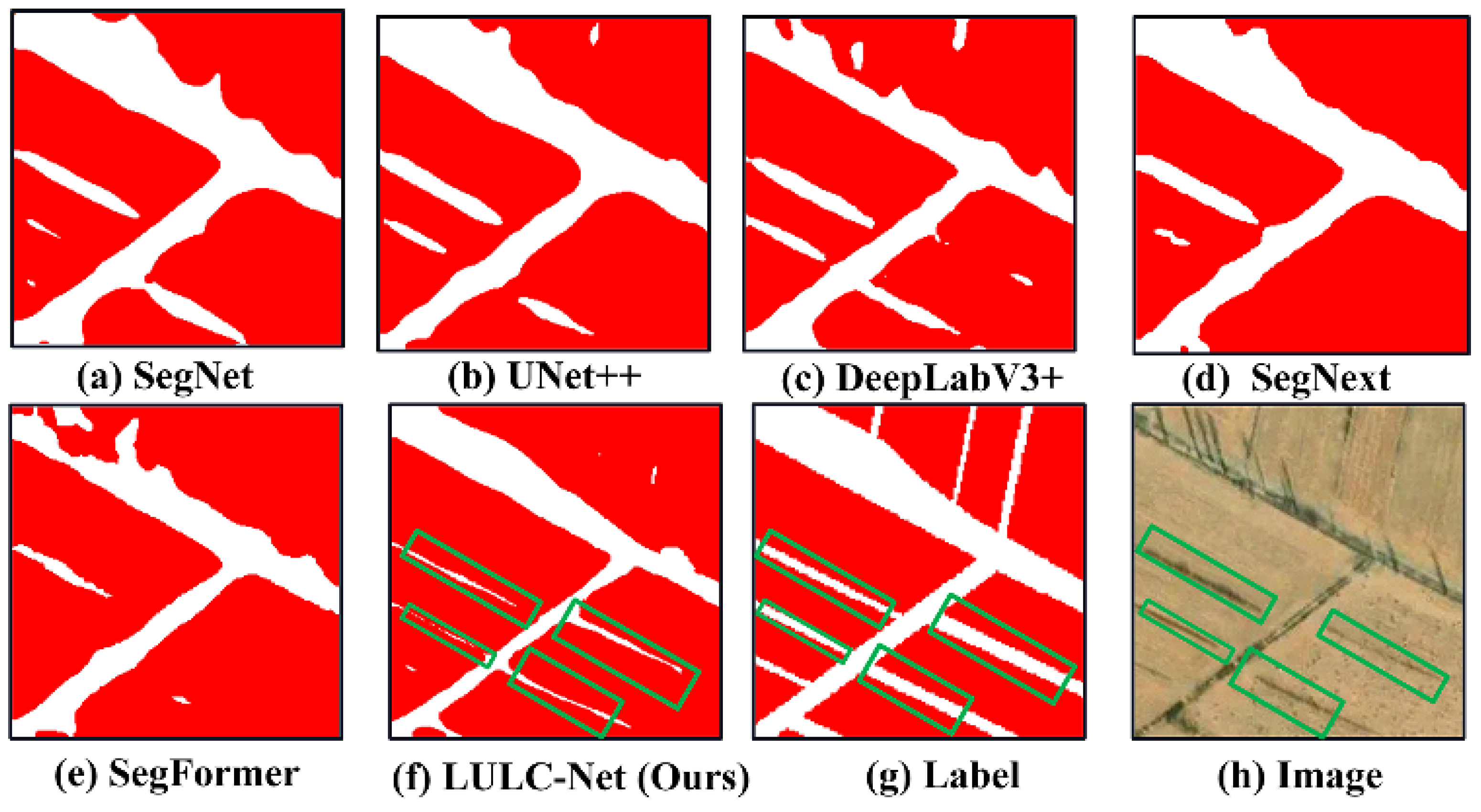
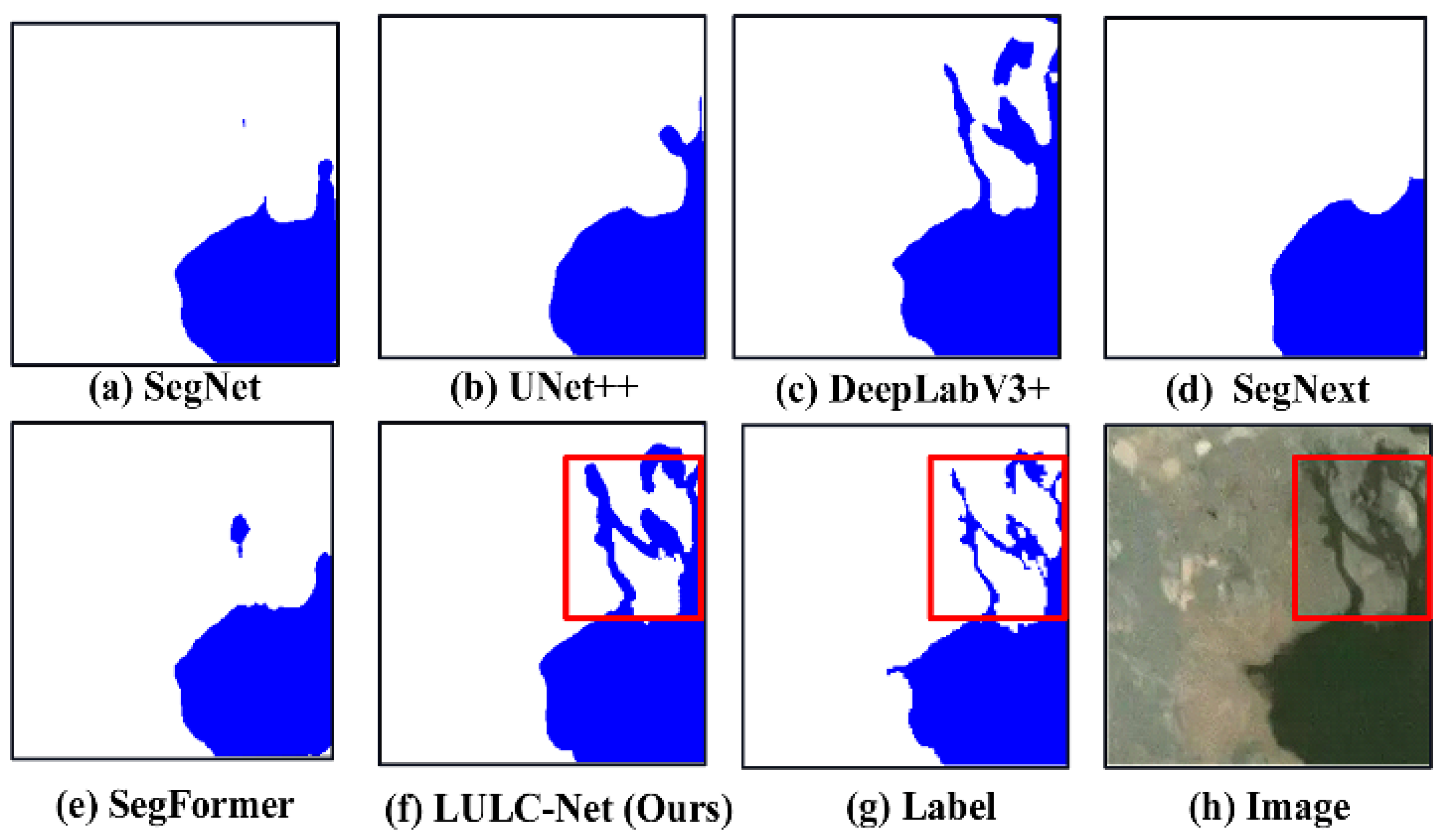
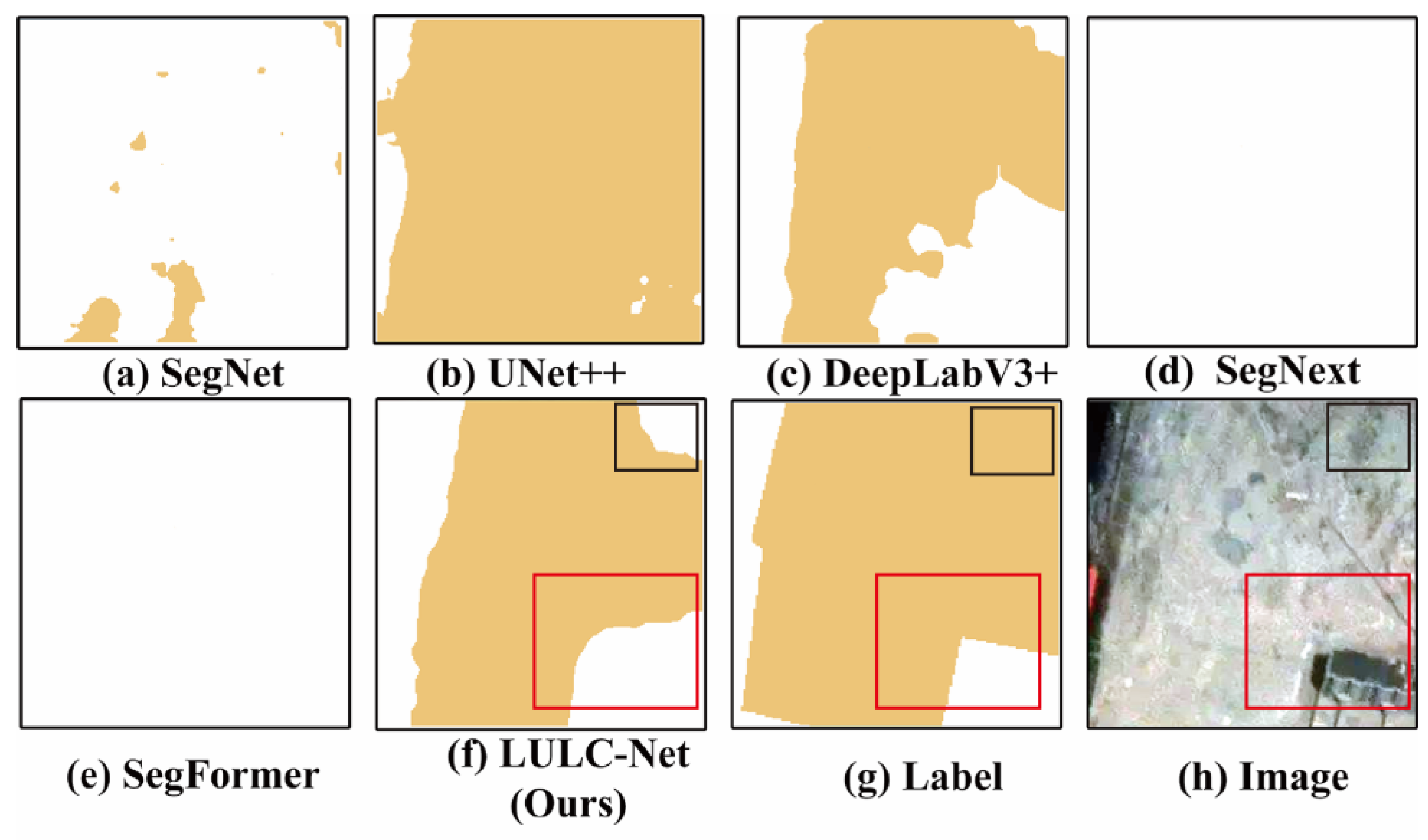
4.5. LULC Segmentation Network Visualization Results

We also demonstrate the model performances through a series of visualizations of qualitative examples to highlight the practical utility of our proposed approach on the LULC dataset in the Circum-Tarim Basin region. The visualization results presented in Figure 9, Figure 10, Figure 11 and Figure 12 clearly show that the LULC segmentation algorithm incorporating the DDPM features exhibits an excellent semantic segmentation performance.
In Figure 9, when the Gobi and farmland features were segmented, our proposed network yields a more straightforward contour definition than the current dominant semantic segmentation models. Similarly, in Figure 10, our approach shows higher sensitivity to the edges of cultivated land due to its incorporation of DDPM features. Our model can segment the precise edge contours consistently with the natural features. These results effectively demonstrate the superior ability of the LULC-SegNet to detect feature boundaries and details by incorporating the DDPM features, ensuring that the segmentation results have recognizable boundary contours.
As shown in Figure 11, the LULC-SegNet shows high sensitivity in recognizing feature boundaries, successfully delineating contours that match the actual labels. As demonstrated in Figure 12, our network is remarkably efficacious in detecting and classifying water bodies and their tiny regions, reproducing the contour features presented by the labels. In Figure 13, urban bare land belongs to a class with imbalanced representation. Convolutional networks based on convolutional structures can detect this category by leveraging convolutional kernels’ local feature extraction capabilities. In contrast, Transformer architecture nets cannot learn the features of imbalanced land cover types due to the limitations in the training dataset size. Additionally, the LULC-SegNet integrates the geometric features of DDPM, enhancing the feature extraction ability of convolutional kernels and thereby effectively identifying land cover morphologies. However, the segmentation performance of the LULC SegNet still needs to be improved because of the impact of class imbalance.
Notably, the river and urban bare land class accounts for a low percentage of pixels in the samples. Other segmentation networks, such as SegFormer, based on the Transformer architecture, often have difficulty effectively performing LULC classification due to the small number of pixels in the samples when handling the class imbalance of the training samples. In contrast, our proposed DDPM feature fusion technique for the category imbalance problem demonstrate excellent segmentation performance when handling feature categories with few pixels. This further highlight that our LULC-SegNet possesses processing capabilities in complex semantic segmentation tasks.

5. Discussion

The central role of the denoising diffusion probabilistic model is to inject Gaussian noise into the original image through the process of forward diffusion. A neural network is then used to predict the amount of noise that is added at each forward diffusion step. The predicted noise is used to perform the opposite denoising process, which is a series of inverse operations to remove noise from the image. During the backward inference process, the DDPM decoder generates rich semantic information closely related to the original image. Our LULC-SegNet network innovatively combines the upstream semantic features generated by the DDPM with the texture features of the original remote sensing image, working to bridge this diffusion generation model to the downstream segmentation task.
Furthermore, by optimizing the semantic information directly generated by the DDPM decoder through the clustering method and attention mechanism, we filter out the redundant noise information and highlight the critical semantic information, which is beneficial to the training efficiency and effectiveness of the whole network. Experiments demonstrate that incorporating the semantic features generated by the decoder in the pre-trained DDPM into the LULC-SegNet can significantly enhance the segmentation ability of the surface boundary contours and the detection sensitivity of tiny regions. It can effectively alleviate the information bottleneck brought by deep convolutional networks and improve the performance of the LULC segmentation. In addition, to overcome the category imbalance in the training dataset, we adopted a generalized weighted loss function strategy, which allows for the network to be trained consistently and efficiently.
The LULC-SegNet has some inevitable limitations. Further optimization is still needed for class-imbalanced samples (few-shot learning). In the attention and clustering module, the K-means clustering algorithm relies on a priori statistics of the entire dataset, and when faced with individual samples, the selection of clusters can affect segmentation performance. Therefore, future work could adopt adaptive clustering algorithms (such as DBSCAN, spectral clustering, fuzzy C-means, and Gaussian mixture models) to aggregate geometric features. Additionally, LULC-SegNet incorporates the extensive decoder of the DDPM, resulting in an inference efficiency lower than that of the segmentation networks based purely on convolutional architectures. This aspect also requires continuous optimization in subsequent work.

6. Conclusions

(1)
In this study, we designed and implemented the LULC semantic segmentation network integrated with the semantic features of the DDPM decoder, alleviating the information bottleneck of deep networks and enhancing the segmentation performance of LULC. The experimental results indicate that (1) the LULC segmentation performance improved. Compared with the mainstream semantic segmentation models, the LULC-SegNet achieved an 80.25% MIOU on the test set, surpassing other models. The network performs well with training samples that have highly imbalanced classes. Visual quality analysis demonstrates that, because of the integration of DDPM’s semantic features, the proposed network can more accurately delineate feature contours and detailed characteristics, significantly improving segmentation accuracy and effectively alleviating the information bottleneck of deep networks.
(2)
The advantages of independent feature extractors are as follows: We demonstrated that the DDPM can function as an independent feature extractor trained using unsupervised methods. This training mechanism avoids dependence on labeled data, making it especially suitable for handling large volumes of remote sensing data. Furthermore, the weights of the upstream diffusion model feature extractor are frozen, and the parameters of the downstream lightweight LULC segmentation model are adjusted, facilitating feature transfer for various types of remote sensing image segmentation.
(3)
We constructed a high-resolution remote sensing image dataset with a class imbalance to meet the requirements of the LULC segmentation tasks, particularly addressing the class imbalance characteristics of the sample categories in the Circum-Tarim region.
The research demonstrates that the LULC-SegNet, integrated with DDPM features, possesses significant advantages in enhancing segmentation performance, reducing dependence on labeled data, and adapting to class imbalance.

Author Contributions

Conceptualization, Z.S. and J.F.; Data curation, Y.Z. (Yuke Zhou); Formal analysis, Y.D.; Funding acquisition, J.F. and Y.Z. (Yuke Zhou); Investigation, Y.D. and Y.Z. (Yi Zhang); Methodology, Z.S. and J.F.; Project administration, J.F.; Resources, Y.Z. (Yuke Zhou) and Y.Z. (Yi Zhang); Software, Z.S., Y.D. and Y.Z. (Yi Zhang); Supervision, J.F.; Validation, Z.S. and Y.D.; Visualization, Z.S.; Writing—Original draft, Z.S., J.F. and Y.D.; Writing—Review and editing, Z.S., J.F. and Y.Z. (Yuke Zhou). All authors have read and agreed to the published version of the manuscript.

Funding

This research was funded by the National Natural Science Foundation of China (No. 42171413), the National Key Research and Development Program (grant no. 2021XJKK0303), and a grant from the State Key Laboratory of Resources and Environmental Information Systems.

Data Availability Statement

The data presented in this study are available upon request from the corresponding author (The data are not publicly available due to privacy.)

Acknowledgments

We would like to thank the State Key Laboratory of Resources and Environmental Information Systems for providing remote sensing images of the Circum-Tarim area. We appreciate the editors and reviewers for their constructive comments and suggestions.

Conflicts of Interest

The authors declare no conflicts of interest.

References

  1. Xie, Y.; Sha, Z.; Yu, M. Remote Sensing Imagery in Vegetation Mapping: A Review. J. Plant Ecol. 2008, 1, 9–23. [Google Scholar] [CrossRef]
  2. Vemuri, R.K.; Reddy, P.C.S.; Puneeth Kumar, B.S.; Ravi, J.; Sharma, S.; Ponnusamy, S. Deep Learning Based Remote Sensing Technique for Environmental Parameter Retrieval and Data Fusion from Physical Models. Arab. J. Geosci. 2021, 14, 1230. [Google Scholar] [CrossRef]
  3. Qi, W. Object Detection in High Resolution Optical Image Based on Deep Learning Technique. Nat. Hazards Res. 2022, 2, 384–392. [Google Scholar] [CrossRef]
  4. Wang, Z.; Wang, J.; Yang, K.; Wang, L.; Su, F.; Chen, X. Semantic Segmentation of High-Resolution Remote Sensing Images Based on a Class Feature Attention Mechanism Fused with Deeplabv3+. Comput. Geosci. 2022, 158, 104969. [Google Scholar] [CrossRef]
  5. Wang, M.; Du, H.; Xu, S.; Surname, G.N. Remote Sensing Image Segmentation of Ground Objects Based on Improved Deeplabv3+. In Proceedings of the 2022 IEEE International Conference on Industrial Technology (ICIT), Shanghai, China, 22–25 August 2022; pp. 1–6. [Google Scholar]
  6. Li, X.; Li, Y.; Ai, J.; Shu, Z.; Xia, J.; Xia, Y. Semantic Segmentation of UAV Remote Sensing Images Based on Edge Feature Fusing and Multi-Level Upsampling Integrated with Deeplabv3. PLoS ONE 2023, 18, e0279097. [Google Scholar] [CrossRef]
  7. Shun, Z.; Li, D.; Jiang, H.; Li, J.; Peng, R.; Lin, B.; Liu, Q.; Gong, X.; Zheng, X.; Liu, T. Research on Remote Sensing Image Extraction Based on Deep Learning. PeerJ Comput. Sci. 2022, 8, e847. [Google Scholar] [CrossRef]
  8. Adegun, A.A.; Fonou Dombeu, J.V.; Viriri, S.; Odindi, J. State-of-the-Art Deep Learning Methods for Objects Detection in Remote Sensing Satellite Images. Sensors 2023, 23, 5849. [Google Scholar] [CrossRef]
  9. Zheng, X.; Huan, L.; Xia, G.-S.; Gong, J. Parsing Very High-Resolution Urban Scene Images by Learning Deep ConvNets with Edge-Aware Loss. ISPRS J. Photogramm. Remote Sens. 2020, 170, 15–28. [Google Scholar] [CrossRef]
  10. Huang, B.; Zhao, B.; Song, Y. Urban Land-Use Mapping Using a Deep Convolutional Neural Network with High Spatial Resolution Multispectral Remote Sensing Imagery. Remote Sens. Environ. 2018, 214, 73–86. [Google Scholar] [CrossRef]
  11. Sertel, E.; Ekim, B.; Ettehadi Osgouei, P.; Kabadayi, M.E. Land Use and Land Cover Mapping Using Deep Learning Based Segmentation Approaches and VHR Worldview-3 Images. Remote Sens. 2022, 14, 4558. [Google Scholar] [CrossRef]
  12. Usmani, M.; Napolitano, M.; Bovolo, F. Towards Global Scale Segmentation with OpenStreetMap and Remote Sensing. ISPRS Open J. Photogramm. Remote Sens. 2023, 8, 100031. [Google Scholar] [CrossRef]
  13. Rousset, G.; Despinoy, M.; Schindler, K.; Mangeas, M. Assessment of Deep Learning Techniques for Land Use Land Cover Classification in Southern New Caledonia. Remote Sens. 2021, 13, 2257. [Google Scholar] [CrossRef]
  14. Zhang, P.; Ke, Y.; Zhang, Z.; Wang, M.; Li, P.; Zhang, S. Urban Land Use and Land Cover Classification Using Novel Deep Learning Models Based on High Spatial Resolution Satellite Imagery. Sensors 2018, 18, 3717. [Google Scholar] [CrossRef]
  15. Ronneberger, O.; Fischer, P.; Brox, T. U-Net: Convolutional Networks for Biomedical Image Segmentation. In Medical Image Computing and Computer-Assisted Intervention—MICCAI 2015, Proceedings of the 18th International Conference, Munich, Germany, 5–9 October 2015; Navab, N., Hornegger, J., Wells, W.M., Frangi, A.F., Eds.; Springer International Publishing: Cham, Switzerland, 2015; pp. 234–241. [Google Scholar]
  16. Clark, A.; Phinn, S.; Scarth, P. Optimised U-Net for Land Use–Land Cover Classification Using Aerial Photography. PFG J. Photogramm. Remote Sens. Geoinf. Sci. 2023, 91, 125–147. [Google Scholar] [CrossRef]
  17. Wang, J.; Yang, M.; Chen, Z.; Lu, J.; Zhang, L. An MLC and U-Net Integrated Method for Land Use/Land Cover Change Detection Based on Time Series NDVI-Composed Image from PlanetScope Satellite. Water 2022, 14, 3363. [Google Scholar] [CrossRef]
  18. Ding, M.; Xiao, B.; Codella, N.; Luo, P.; Wang, J.; Yuan, L. DaViT: Dual Attention Vision Transformers. In Proceedings of the 17th European Conference, Tel Aviv, Israel, 23–27 October 2022; Avidan, S., Brostow, G., Cissé, M., Farinella, G.M., Hassner, T., Eds.; Springer Nature Switzerland: Cham, Switzerland, 2022; pp. 74–92. [Google Scholar]
  19. Dosovitskiy, A.; Beyer, L.; Kolesnikov, A.; Weissenborn, D.; Zhai, X.; Unterthiner, T.; Dehghani, M.; Minderer, M.; Heigold, G.; Gelly, S.; et al. An Image Is Worth 16 × 16 Words: Transformers for Image Recognition at Scale. arXiv 2021, arXiv:2010.11929. [Google Scholar]
  20. Zheng, W.; Feng, J.; Gu, Z.; Zeng, M. A Stage-Adaptive Selective Network with Position Awareness for Semantic Segmentation of LULC Remote Sensing Images. Remote Sens. 2023, 15, 2811. [Google Scholar] [CrossRef]
  21. Scheibenreif, L.; Hanna, J.; Mommert, M.; Borth, D. Self-Supervised Vision Transformers for Land-Cover Segmentation and Classification. In Proceedings of the 2022 IEEE/CVF Conference on Computer Vision and Pattern Recognition Workshops (CVPRW), New Orleans, LA, USA, 18–24 June 2022; pp. 1421–1430. [Google Scholar]
  22. Tishby, N.; Zaslavsky, N. Deep Learning and the Information Bottleneck Principle. In Proceedings of the 2015 IEEE Information Theory Workshop (ITW), Jerusalem, Israel, 26 April–1 May 2015; pp. 1–5. [Google Scholar]
  23. Saharia, C.; Chan, W.; Chang, H.; Lee, C.A.; Ho, J.; Salimans, T.; Fleet, D.J.; Norouzi, M. Palette: Image-to-Image Diffusion Models. In Proceedings of the SIGGRAPH‘22: Special Interest Group on Computer Graphics and Interactive Techniques Conference, Vancouver, BC, Canada, 7–11 August 2022. [Google Scholar]
  24. Saharia, C.; Ho, J.; Chan, W.; Salimans, T.; Fleet, D.J.; Norouzi, M. Image Super-Resolution via Iterative Refinement. IEEE Trans. Pattern Anal. Mach. Intell. 2023, 45, 4713–4726. [Google Scholar] [CrossRef]
  25. Karras, T.; Aila, T.; Laine, S.; Lehtinen, J. Progressive Growing of GANs for Improved Quality, Stability, and Variation. arXiv 2017, arXiv:1710.10196. [Google Scholar]
  26. Menick, J.; Kalchbrenner, N. Generating High Fidelity Images with Subscale Pixel Networks and Multidimensional Upscaling. arXiv 2018, arXiv:1812.01608. [Google Scholar]
  27. Lin, C.-H.; Yumer, E.; Wang, O.; Shechtman, E.; Lucey, S. ST-GAN: Spatial Transformer Generative Adversarial Networks for Image Compositing. In Proceedings of the 2018 IEEE/CVF Conference on Computer Vision and Pattern Recognition, Salt Lake City, UT, USA, 18–23 June 2018; pp. 9455–9464. [Google Scholar]
  28. Goodfellow, I.J.; Pouget-Abadie, J.; Mirza, M.; Xu, B.; Warde-Farley, D.; Ozair, S.; Courville, A.; Bengio, Y. Generative Adversarial Nets. In Advances in Neural Information Processing Systems 27, Proceedings of the Annual Conference on Neural Information Processing Systems, Montreal, QC, Canada, 8–13 December 2014; MIT Press: Cambridge, MA, USA, 2014; pp. 2672–2680. [Google Scholar]
  29. Kingma, D.P.; Welling, M. Auto-Encoding Variational Bayes. arXiv 2013, arXiv:1312.6114. [Google Scholar]
  30. Kingma, D.P.; Welling, M. An Introduction to Variational Autoencoders. FNT Mach. Learn. 2019, 12, 307–392. [Google Scholar] [CrossRef]
  31. Souly, N.; Spampinato, C.; Shah, M. Semi Supervised Semantic Segmentation Using Generative Adversarial Network. In Proceedings of the 2017 IEEE International Conference on Computer Vision (ICCV), Venice, Italy, 22–29 October 2017; pp. 5689–5697. [Google Scholar]
  32. Ho, J.; Jain, A.; Abbeel, P. Denoising Diffusion Probabilistic Models. In Advances in Neural Information Processing Systems 33, Proceedings of the Annual Conference on Neural Information Processing Systems (NeurIPS 2020), Virtual, 6–12 December 2020; MIT Press: Cambridge, MA, USA, 2020. [Google Scholar]
  33. Gedara Chaminda Bandara, W.; Gopalakrishnan Nair, N.; Patel, V.M. DDPM-CD: Denoising Diffusion Probabilistic Models as Feature Extractors for Change Detection. arXiv 2022, arXiv:2206.11892. [Google Scholar]
  34. Yao, J.; Chen, Y.; Guan, X.; Zhao, Y.; Chen, J.; Mao, W. Recent Climate and Hydrological Changes in a Mountain–Basin System in Xinjiang, China. Earth-Sci. Rev. 2022, 226, 103957. [Google Scholar] [CrossRef]
  35. Hong, Z.; Jian-Wei, W.; Qiu-Hong, Z.; Yun-Jiang, Y. A Preliminary Study of Oasis Evolution in the Tarim Basin, Xinjiang, China. J. Arid Environ. 2003, 55, 545–553. [Google Scholar] [CrossRef]
  36. Karras, T.; Aittala, M.; Aila, T.; Laine, S. Elucidating the Design Space of Diffusion-Based Generative Models. arXiv 2022, arXiv:2206.00364. [Google Scholar]
  37. Fan, J.; Shi, Z.; Ren, Z.; Zhou, Y.; Ji, M. DDPM-SegFormer: Highly Refined Feature Land Use and Land Cover Segmentation with a Fused Denoising Diffusion Probabilistic Model and Transformer. Int. J. Appl. Earth Obs. Geoinf. 2024, 133, 104093. [Google Scholar] [CrossRef]
  38. Saharia, C.; Ho, J.; Chan, W.; Salimans, T.; Fleet, D.J.; Norouzi, M. Image Super-Resolution via Iterative Refinement. arXiv 2021, arXiv:2104.07636. [Google Scholar]
  39. Baranchuk, D.; Rubachev, I.; Voynov, A.; Khrulkov, V.; Babenko, A. Label-Efficient Semantic Segmentation with Diffusion Models. arXiv 2021, arXiv:2112.03126. [Google Scholar]
  40. Li, H.; Yang, Y.; Chang, M.; Chen, S.; Feng, H.; Xu, Z.; Li, Q.; Chen, Y. SRDiff: Single Image Super-Resolution with Diffusion Probabilistic Models. Neurocomputing 2022, 479, 47–59. [Google Scholar] [CrossRef]
  41. Li, X.; Wang, W.; Hu, X.; Yang, J. Selective Kernel Networks. In Proceedings of the 2019 IEEE/CVF Conference on Computer Vision and Pattern Recognition (CVPR), Long Beach, CA, USA, 15–20 June 2019; pp. 510–519. [Google Scholar]
  42. Fu, J.; Liu, J.; Tian, H.; Li, Y. Dual Attention Network for Scene Segmentation. In Proceedings of the 2019 IEEE/CVF Conference on Computer Vision and Pattern Recognition (CVPR), Long Beach, CA, USA, 15–20 June 2019. [Google Scholar] [CrossRef]
  43. Guo, H.; Jin, X.; Jiang, Q.; Wozniak, M.; Wang, P.; Yao, S. DMF-Net: A Dual Remote Sensing Image Fusion Network Based on Multiscale Convolutional Dense Connectivity with Performance Measure. IEEE Trans. Instrum. Meas. 2024, 73, 1–15. [Google Scholar] [CrossRef]
  44. Chen, L.-C.; Zhu, Y.; Papandreou, G.; Schroff, F.; Adam, H. Encoder-Decoder with Atrous Separable Convolution for Semantic Image Segmentation. In Proceedings of the European Conference on Computer Vision (ECCV 2018), Munich, Germany, 8–14 September 2018; Ferrari, V., Hebert, M., Sminchisescu, C., Weiss, Y., Eds.; Springer International Publishing: Cham, Switzerland, 2018; pp. 833–851. [Google Scholar]
  45. Roy, A.G.; Navab, N.; Wachinger, C. Concurrent Spatial and Channel ‘Squeeze & Excitation’ in Fully Convolutional Networks. In Medical Image Computing and Computer Assisted Intervention (MICCAI 2018), Proceedings of the 21st International Conference, Granada, Spain, 16–20 September 2018; Frangi, A.F., Schnabel, J.A., Davatzikos, C., Alberola-López, C., Fichtinger, G., Eds.; Springer International Publishing: Cham, Switzerland, 2018; Volume 11070, pp. 421–429. [Google Scholar]
  46. Hu, J.; Shen, L.; Albanie, S.; Sun, G.; Wu, E. Squeeze-and-Excitation Networks. IEEE Trans. Pattern Anal. Mach. Intell. 2020, 42, 2011–2023. [Google Scholar] [CrossRef] [PubMed]
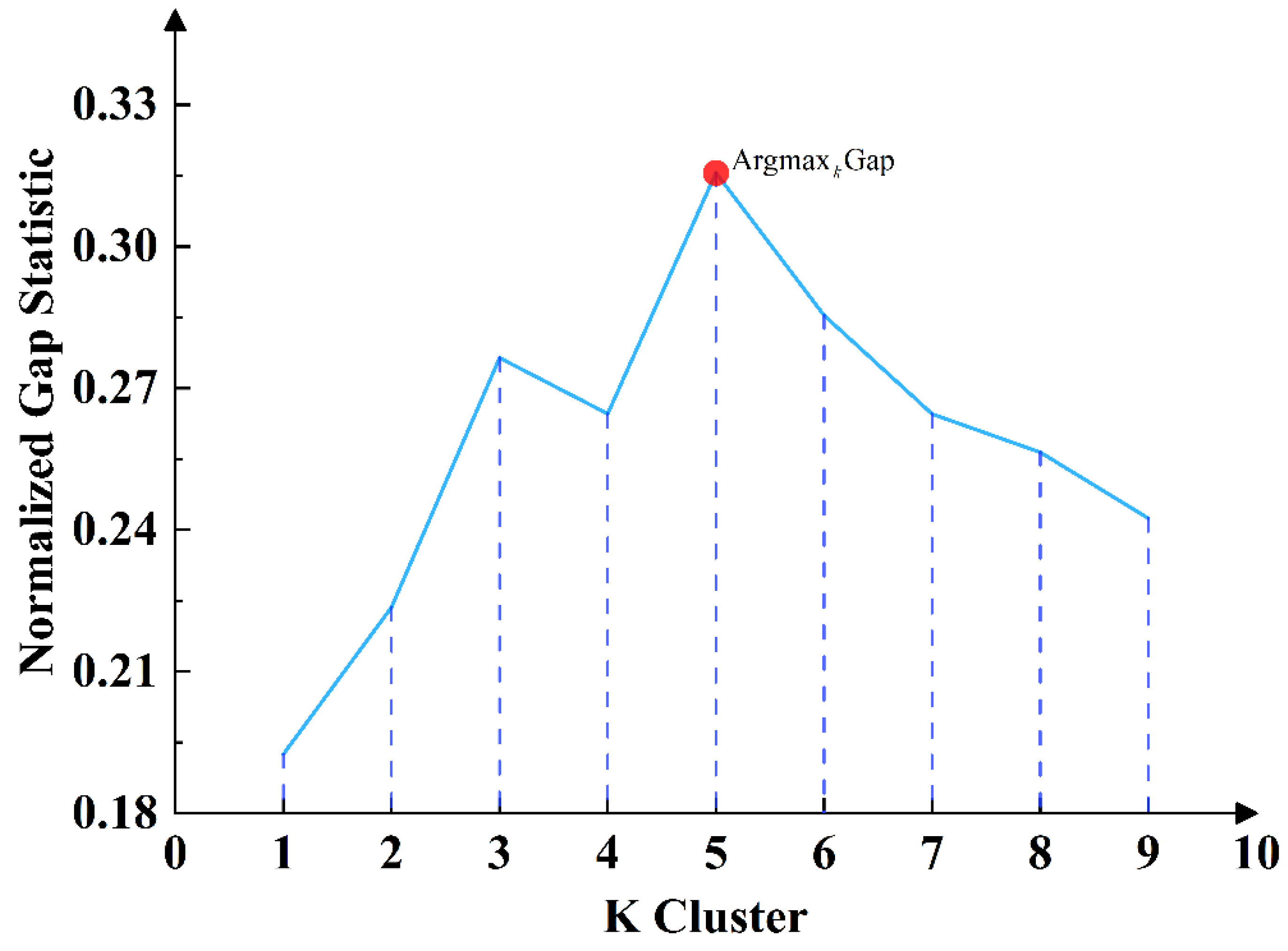
  47. Tibshirani, R.; Walther, G.; Hastie, T. Estimating the Number of Clusters in a Data Set Via the Gap Statistic. J. R. Stat. Soc. Ser. B Stat. Methodol. 2001, 63, 411–423. [Google Scholar] [CrossRef]
  48. Lin, T.-Y.; Goyal, P.; Girshick, R.; He, K.; Dollár, P. Focal Loss for Dense Object Detection. In Proceedings of the 2017 IEEE International Conference on Computer Vision (ICCV), Venice, Italy, 22–29 October 2017; pp. 2999–3007. [Google Scholar]
  49. Milletari, F.; Navab, N.; Ahmadi, S.-A. V-Net: Fully Convolutional Neural Networks for Volumetric Medical Image Segmentation. In Proceedings of the 2016 Fourth International Conference on 3D Vision (3DV), Stanford, CA, USA, 25–28 October 2016; pp. 565–571. [Google Scholar]
  50. Zhang, Y.; Fan, J.; Zhang, M.; Shi, Z.; Liu, R.; Guo, B. A Recurrent Adaptive Network: Balanced Learning for Road Crack Segmentation with High-Resolution Images. Remote Sens. 2022, 14, 3275. [Google Scholar] [CrossRef]
  51. Zhang, Z.; Sabuncu, M.R. Generalized Cross Entropy Loss for Training Deep Neural Networks with Noisy Labels. In Advances in Neural Information Processing Systems 31, Proceedings of the Annual Conference on Neural Information Processing Systems 2018 (NeurIPS 2018), Montréal, QC, Canada, 3–8 December 2018; Curran Associates Inc.: Red Hook, NY, USA, 2018; pp. 8792–8802. [Google Scholar]
  52. Dickson, M.C.; Bosman, A.S.; Malan, K.M. Hybridised Loss Functions for Improved Neural Network Generalisation. In Pan-African Artificial Intelligence and Smart Systems, Procceedings of the First International Conference (PAAISS 2021), Windhoek, Namibia, 6–8 September 2021; Ngatched, T.M.N., Woungang, I., Eds.; Springer International Publishing: Cham, Switzerland, 2022; pp. 169–181. [Google Scholar]
  53. Jadon, S. A Survey of Loss Functions for Semantic Segmentation. In Proceedings of the 2020 IEEE Conference on Computational Intelligence in Bioinformatics and Computational Biology (CIBCB), Via del Mar, Chile, 27–29 October 2020; pp. 1–7. [Google Scholar]
  54. Kalsotra, R.; Arora, S. Performance Analysis of U-Net with Hybrid Loss for Foreground Detection. Multimed. Syst. 2023, 29, 771–786. [Google Scholar] [CrossRef]
  55. Cheng, Q.; Li, H.; Wu, Q.; Ngi Ngan, K. Hybrid-Loss Supervision for Deep Neural Network. Neurocomputing 2020, 388, 78–89. [Google Scholar] [CrossRef]
  56. Yeung, M.; Sala, E.; Schönlieb, C.-B.; Rundo, L. Unified Focal Loss: Generalising Dice and Cross Entropy-Based Losses to Handle Class Imbalanced Medical Image Segmentation. Comput. Med. Imaging Graph. 2022, 95, 102026. [Google Scholar] [CrossRef]
  57. Goodfellow, I.; Bengio, Y.; Courville, A. Deep Learning; MIT Press: Cambridge, MA, USA, 2016; ISBN 978-0-262-33737-3. [Google Scholar]
  58. Bengio, Y.; Simard, P.; Frasconi, P. Learning Long-Term Dependencies with Gradient Descent Is Difficult. IEEE Trans. Neural Netw. 1994, 5, 157–166. [Google Scholar] [CrossRef]
  59. Krizhevsky, A.; Sutskever, I.; Hinton, G.E. ImageNet Classification with Deep Convolutional Neural Networks. In Advances in Neural Information Processing Systems 25, Proceedings of the 26th Annual Conference on Neural Information Processing Systems 2012, Lake Tahoe, NV, USA, 3–6 December 2012; Curran Associates, Inc.: Red Hook, NY, USA, 2012; Volume 25. [Google Scholar]
  60. Li, X.; Wang, W.; Wu, L.; Chen, S.; Hu, X.; Li, J.; Tang, J.; Yang, J. Generalized Focal Loss: Learning Qualified and Distributed Bounding Boxes for Dense Object Detection. In Advances in Neural Information Processing Systems 33, Proceedings of the Annual Conference on Neural Information Processing Systems 2020 (NeurIPS 2020), Virtual, 6–12 December 2020; Curran Associates, Inc.: Red Hook, NY, USA, 2020; Volume 33, pp. 21002–21012. [Google Scholar]
  61. Qiu, S.; Cheng, X.; Lu, H.; Zhang, H.; Wan, R.; Xue, X.; Pu, J. Subclassified Loss: Rethinking Data Imbalance from Subclass Perspective for Semantic Segmentation. IEEE Trans. Intell. Veh. 2024, 9, 1547–1558. [Google Scholar] [CrossRef]
  62. Sudre, C.H.; Li, W.; Vercauteren, T.; Ourselin, S.; Jorge Cardoso, M. Generalised Dice Overlap as a Deep Learning Loss Function for Highly Unbalanced Segmentations. In Deep Learning in Medical Image Analysis and Multimodal Learning for Clinical Decision Support; Cardoso, M.J., Arbel, T., Carneiro, G., Syeda-Mahmood, T., Tavares, J.M.R.S., Moradi, M., Bradley, A., Greenspan, H., Papa, J.P., Madabhushi, A., et al., Eds.; Lecture Notes in Computer Science; Springer International Publishing: Cham, Switzerland, 2017; Volume 10553, pp. 240–248. ISBN 978-3-319-67557-2. [Google Scholar]
  63. Chen, L.-C.; Papandreou, G.; Schroff, F.; Adam, H. Rethinking Atrous Convolution for Semantic Image Segmentation. arXiv 2017, arXiv:1706.05587. [Google Scholar]
  64. Yu, F.; Koltun, V. Multi-Scale Context Aggregation by Dilated Convolutions. arXiv 2016, arXiv:1511.07122. [Google Scholar]
  65. Badrinarayanan, V.; Kendall, A.; Cipolla, R. SegNet: A Deep Convolutional Encoder-Decoder Architecture for Image Segmentation. IEEE Trans. Pattern Anal. Mach. Intell. 2017, 39, 2481–2495. [Google Scholar] [CrossRef] [PubMed]
  66. Zhou, Z.; Rahman Siddiquee, M.M.; Tajbakhsh, N.; Liang, J. Unet++: A Nested u-Net Architecture for Medical Image Segmentation. In Deep Learning in Medical Image Analysis and Multimodal Learning for Clinical Decision Support, Proceedings of the 4th International Workshop, DLMIA 2018, and 8th International Workshop, ML-CDS 2018, Held in Conjunction with MICCAI 2018, Granada, Spain, 20 September 2018; Springer: Cham, Switzerland, 2018; pp. 3–11. [Google Scholar]
  67. Guo, M.-H.; Lu, C.-Z.; Hou, Q.; Liu, Z.; Cheng, M.-M.; Hu, S.-M. Segnext: Rethinking Convolutional Attention Design for Semantic Segmentation. Adv. Neural Inf. Process. Syst. 2022, 35, 1140–1156. [Google Scholar]
  68. Xie, E.; Wang, W.; Yu, Z.; Anandkumar, A.; Alvarez, J.M.; Luo, P. SegFormer: Simple and Efficient Design for Semantic Segmentation with Transformers. Adv. Neural Inf. Process. Syst. 2021, 34, 12077–12090. [Google Scholar] [CrossRef]
Figure 1. LULC-SegNet network structure: The network consists of an encoder–decoder architecture, where the encoder incorporates an attention module, an attention and clustering module, a CNN feature extractor, and a DDPM feature extractor. The decoder is designed to integrate these features to accomplish semantic segmentation. (a–d) Multi-scale features extracted from the SR3-Decoder.
Remotesensing 16 04573 g001
Figure 2. Circum-Tarim Basin Region LULC Dataset.
Remotesensing 16 04573 g002
Figure 3. Forward (solid arrows is additive noise) and reverse (dotted arrows is denoising noise) processes of the diffusion modeling [37].
Remotesensing 16 04573 g003
Figure 4. Estimation of  ϵ θ ( x t , t )  via the SR3, where  X 0  is the original remote sensing image,  X t  is the image with Gaussian noise added at time t,  L o s s  is the loss function,  ϵ  is the Gaussian noise added in the forward process,  ϵ θ  is the noise predicted by the denoising network,  θ  is the denoising network parameters,  α  is the noise intensity, and  x ^  is the input image restored by SR3.
Remotesensing 16 04573 g004
Figure 5. Circum-Tarim Basin Region LULC Dataset extracted samples under different K-clusters for the gap statistic. The maximum value of the gap statistic when K-cluster = 5 can be considered the best K-means clustering algorithm grouping.
Remotesensing 16 04573 g005
Figure 6. Feature image of the diffusion model after K-clustering (1, 2, 3, 4, 5, and 6) with features after applying space and channel attention.
Remotesensing 16 04573 g006
Figure 7. The (af) subfigures of semantic features obtained after clustering the noise points (K-cluster = 5) with the original image, the red boxes are specific semantic features.
Remotesensing 16 04573 g007
Figure 8. (a,b) The dynamics of the loss curves for the training set and the IOU curves for the validation set using the SegNet, UNet++, DeepLabV3+, SegNext, and SegFormer architectures throughout the training epochs. (c,d) The changes in the training loss and the validation IOU for our LULC-SegNet model. The progressions of these curves provide insightful indications of each network’s learning behavior and convergence stability over the course of training, thereby enabling the model performance consistency to be rigorously assessed across the training and validation datasets.
Remotesensing 16 04573 g008
Figure 9. The comparative effect of the different SOTA segmentation methods on the LULC dataset in the Tarim Basin area: (a) SegNet; (b) UNet++; (c) DeepLabV3+; (d) SegNext; (e) SegFormer; (f) LULC-SegNet (ours) (g) label (ground truth); (h) image (remote sensing images). The LULC-SegNet can better distinguish farmland (red) from the Gobi (green) at the boundary by adding the DDPM features, the boxes (blue) are typical LULC segmentation comparison results.
Remotesensing 16 04573 g009
Figure 10. The comparative effect of different SOTA segmentation methods on the LULC dataset in the Tarim Basin area. The LULC-SegNet showed a better performance in dividing the farmland (red), the boxes (green) are typical LULC segmentation comparison results.
Remotesensing 16 04573 g010
Figure 11. The comparative effect of the different SOTA segmentation methods on the LULC dataset in the Tarim Basin area. The LULC-SegNet showed a better performance in dividing the Gobi (green), the boxes (red) are typical LULC segmentation comparison results.
Remotesensing 16 04573 g011
Figure 12. The comparative effect of the different SOTA segmentation methods on the LULC dataset in the Tarim Basin area. The LULC-SegNet showed a better performance in dividing the river (blue), the boxes (red) are typical LULC segmentation comparison results.
Remotesensing 16 04573 g012
Figure 13. The comparative effect of different SOTA segmentation methods on the LULC dataset in the Tarim Basin area. The LULC-SegNet showed better a performance in dividing urban bare land (yellow), the boxes (red) are typical LULC segmentation comparison results and the boxes (black) are the result of segmentation that needed to be improved.
Remotesensing 16 04573 g013
Table 1. The numbers land cover class pixels in the LULC dataset samples.
Land Cover CategoryNumber of Pixels
River1,409,772
Urban bare land37,132,400
Gobi81,839,600
Woodland125,038,000
Background360,187,000
Cropland605,957,000
Total1,211,563,772
Table 2. ACM ablation experiment’s quantitative results.
Ablation ExperimentClustering ModuleClustering Module + SK-Attention
MIOUPAF1 ScoreMIOUPAF1 Score
No K-means Clustering60.2578.8778.2664.2279.2579.03
K-means Clustering
(K-cluster = 1)
60.0279.4679.3663.5679.6679.65
K-means Clustering
(K-cluster = 2)
61.3880.6379.0162.6580.5679.96
K-means Clustering
(K-cluster = 3)
65.2380.0678.9268.7880.6378.65
K-means Clustering
(K-cluster = 4)
69.5684.7883.5675.6588.7886.56
K-means Clustering
(K-cluster = 5)
76.5689.5688.2280.2593.9291.92
K-means Clustering
(K-cluster = 6)
72.5689.0687.9674.5690.0587.06
K-means Clustering
(K-cluster = 7)
71.6589.2886.6577.6589.0388.36
K-means Clustering
(K-cluster = 8)
72.8882.7880.5676.5684.6583.39
K-means Clustering
(K-cluster = 9)
69.5681.3580.0170.6580.6579.65
The values in bold are the best value in the experiment.
Table 3. LULC segmentation network ablation results.
Ablation StudyMIOUPAF1 Score
CNN Feature Extraction72.6590.2589.63
CNN Feature Extraction + Attention Module (SK-Attention)72.2292.6392.87
ACM (K-cluster = 5) + CNN Feature Extraction79.2592.2291.64
ACM (K-cluster = 5) + CNN Feature Extraction + Attention Module (SK-Attention)80.2593.9292.92
All values are in %. Higher IOU and F1 score values indicate a good LULC segmentation performance, the values in bold are the best value in the experiment.
Table 4. The MIOU (%) and F1 scores (%) for each category of various segmentation models on the LULC dataset within the Circum-Tarim Basin region, as well as the inference efficiency (FPS) observed in the experiments. Using the same test dataset, we conducted permutation tests on the metrics of the LULC-SegNet compared to other segmentation models.
Urban Bare LandWoodlandGobiRiverCroplandBackgroundMIOUF1 ScoreFPS
SegNet [65]49.03 *78.37 *70.15 *45.22 *83.68 *71.77 *66.37 *90.26 *29.85 *
UNet++ [66]53.06 *81.11 *72.63 *51.89 *88.4574.2670.23 *91.5639.27 *
DeepLabV3+ [44]50.06 *84.22 *70.29 *63.32 *85.5573.4671.15 *93.3932.65 *
SegNext [67]53.91 *91.5283.0459.14 *87.29 *73.574.73 *93.0113.25
SegFormer [68]54.14 *92.3287.1363.01 *88.0475.2476.81 *93.457.32 *
LULC-SegNet (Ours)59.1493.2685.6873.6791.3278.4180.2593.9214.21
Higher IOU and F1 score values indicate a good LULC segmentation performance. * If p < 0.05, the sample is significantly different, the values in bold are the best value in the experiment.
Disclaimer/Publisher’s Note: The statements, opinions and data contained in all publications are solely those of the individual author(s) and contributor(s) and not of MDPI and/or the editor(s). MDPI and/or the editor(s) disclaim responsibility for any injury to people or property resulting from any ideas, methods, instructions or products referred to in the content.

