
Deep Learning Integration of Multi-Model Forecast Precipitation Considering Long Lead Times


Abstract
1. Introduction
- (1)
- The forecast precipitation accuracy of several common numerical weather prediction models was evaluated under different lead times, and the high-accuracy ones were selected as inputs for integration models.
- (2)
- To utilize the power of deep learning to improve forecasting precipitation accuracy, a novel method for multi-model forecast precipitation integration considering long lead times was proposed based on the attention mechanism and a long short-term memory neural network.
- (3)
- The accuracy of integrated forecast precipitation was systematically evaluated from the perspective of point precipitation accuracy and applicability in streamflow forecast, and the superiority of deep learning in multi-model forecast precipitation integration was explained.
2. Study Area and Data
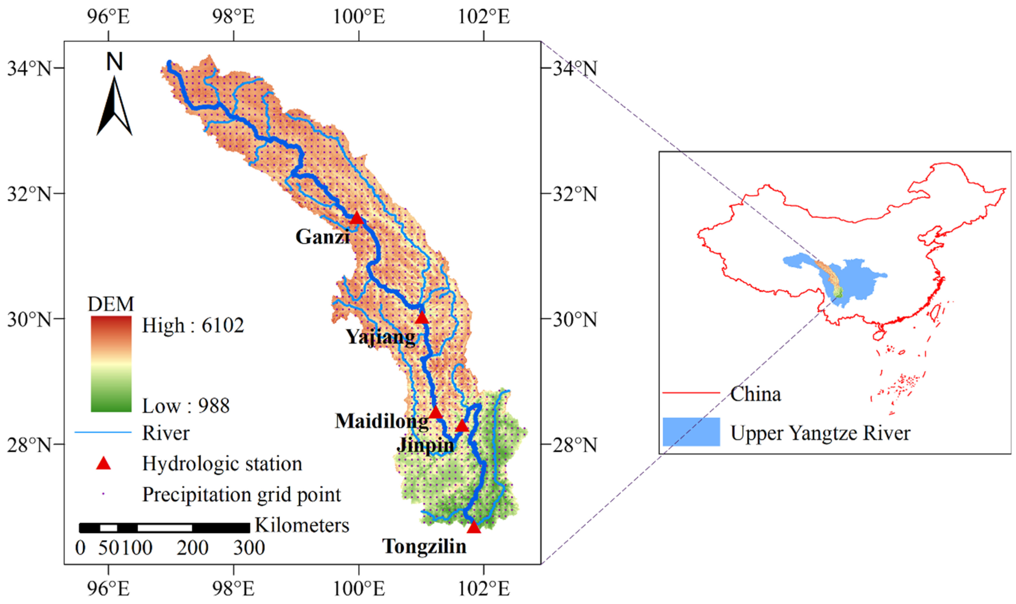
2.1. Study Area
2.2. Data Used
- (1)
- Observed precipitation
- (2)
- Forecast precipitation
- (3)
- Restored streamflow
3. Methodology
3.1. General Modeling Ideas for Multi-Model Forecast Precipitation Integration
3.2. Framework for Multi-Model Forecast Precipitation Integration Considering Long Lead Times
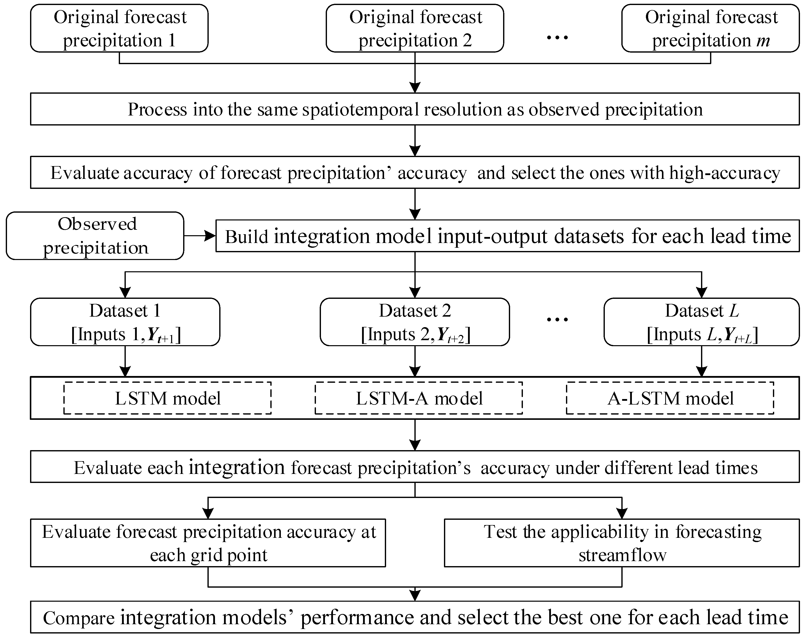
- (1)
- Data collection and processing: Firstly, forecast precipitation from multiple numerical weather prediction models was collected under different lead times. Secondly, it was processed into the same spatiotemporal resolution as the observed precipitation. Finally, its accuracy was evaluated, and the forecast precipitation of high-precision models was selected under different lead times.
- (2)
- Model input-output datasets building: For each lead time, model input–output datasets were built by using the forecast precipitation of high-precision models and integrated forecast precipitation at the current time as inputs and outputs. Each dataset was divided into a training set and a validation set.
- (3)
- Integration model training: Three multi-model forecast precipitation integration models (LSTM, LSTM-A, and A-LSTM) were built by introducing the attention mechanism and LSTM, based on Equations (1)–(3). Based on the training set, the optimal hyperparameter combinations of each integration model were obtained through the Bayesian optimization algorithm under different lead times.
- (4)
- Comparison of models’ performance: Each integrated forecast precipitation was obtained by driving the trained integration models with test sets under different lead times. Their precipitation forecast accuracy and applicability for forecasting streamflow were evaluated to compare the advantages and disadvantages of each integration model and select the optimal integration model for each lead time.
3.3. Models
3.3.1. Attention Mechanism
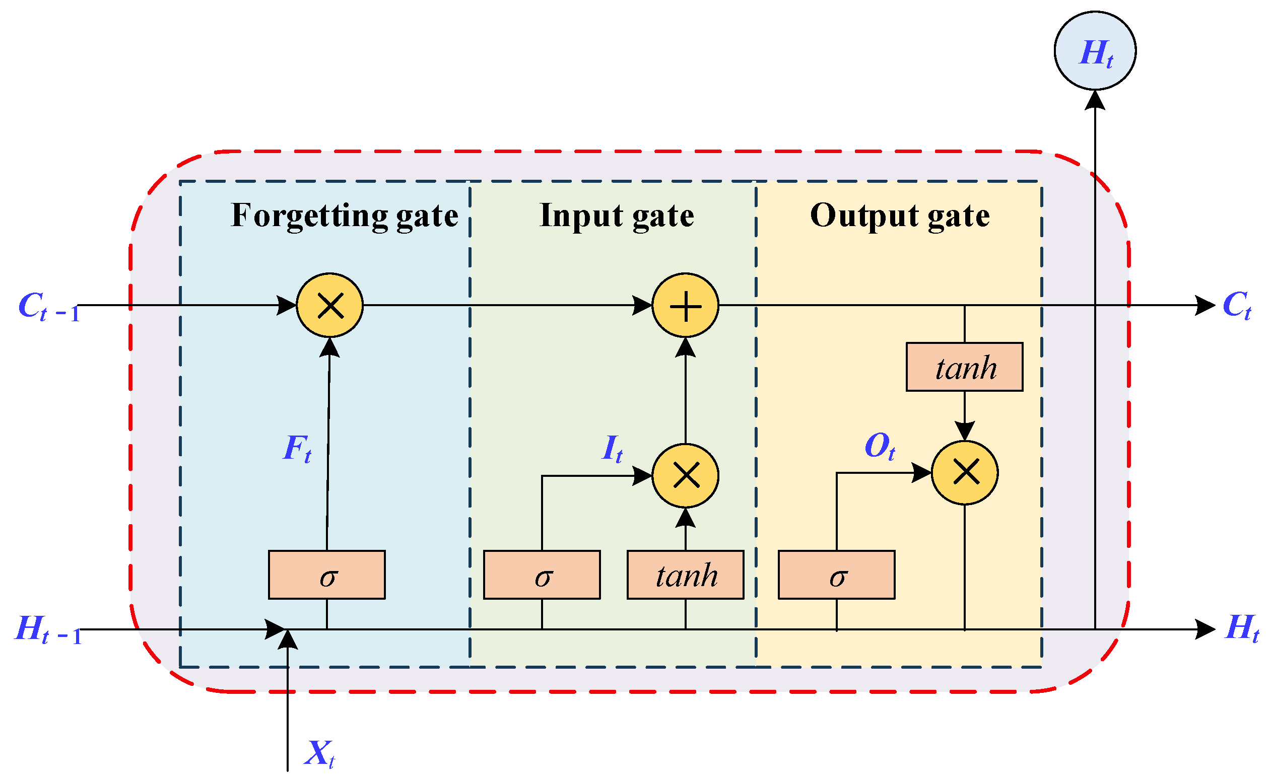
3.3.2. LSTM
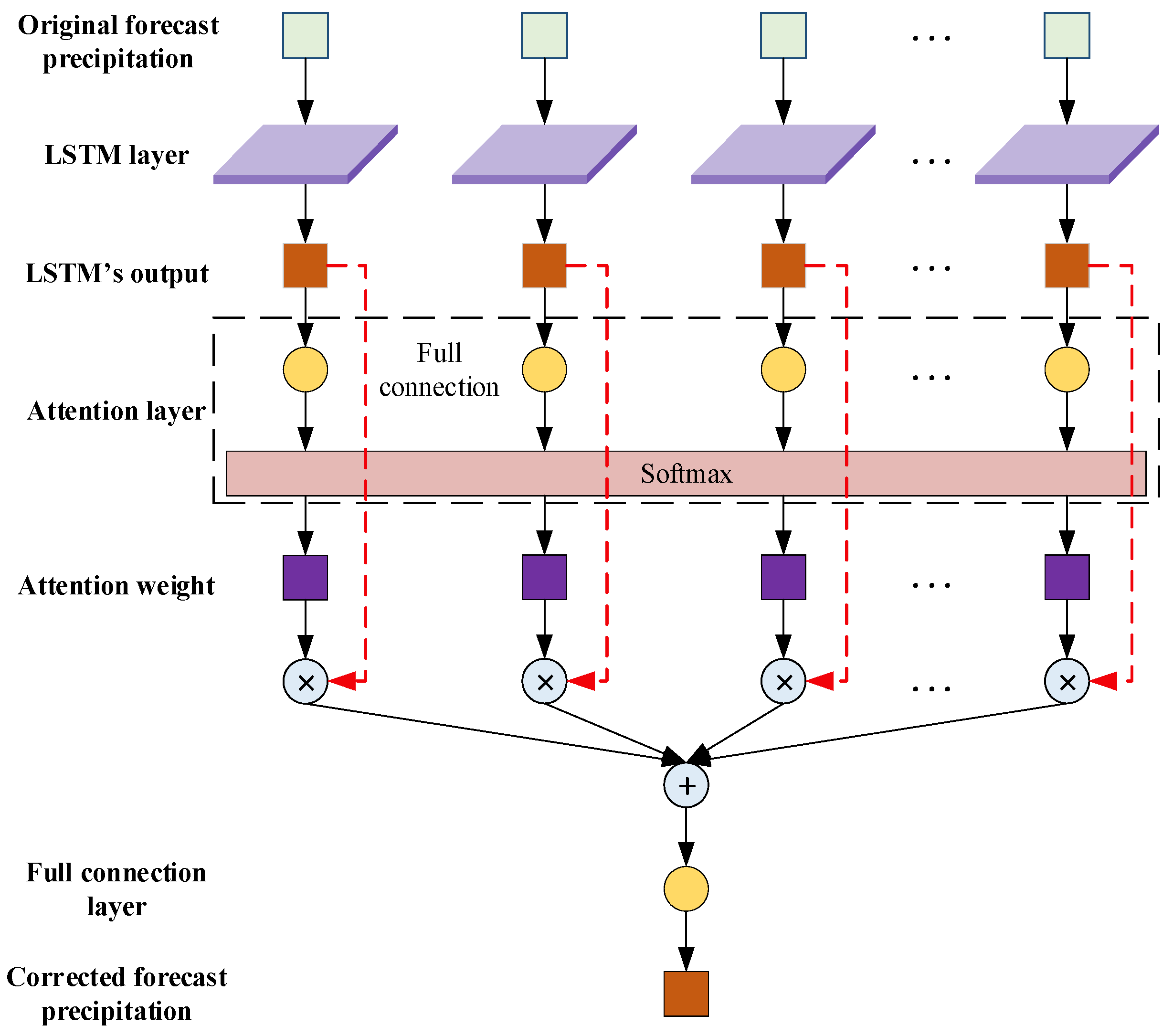
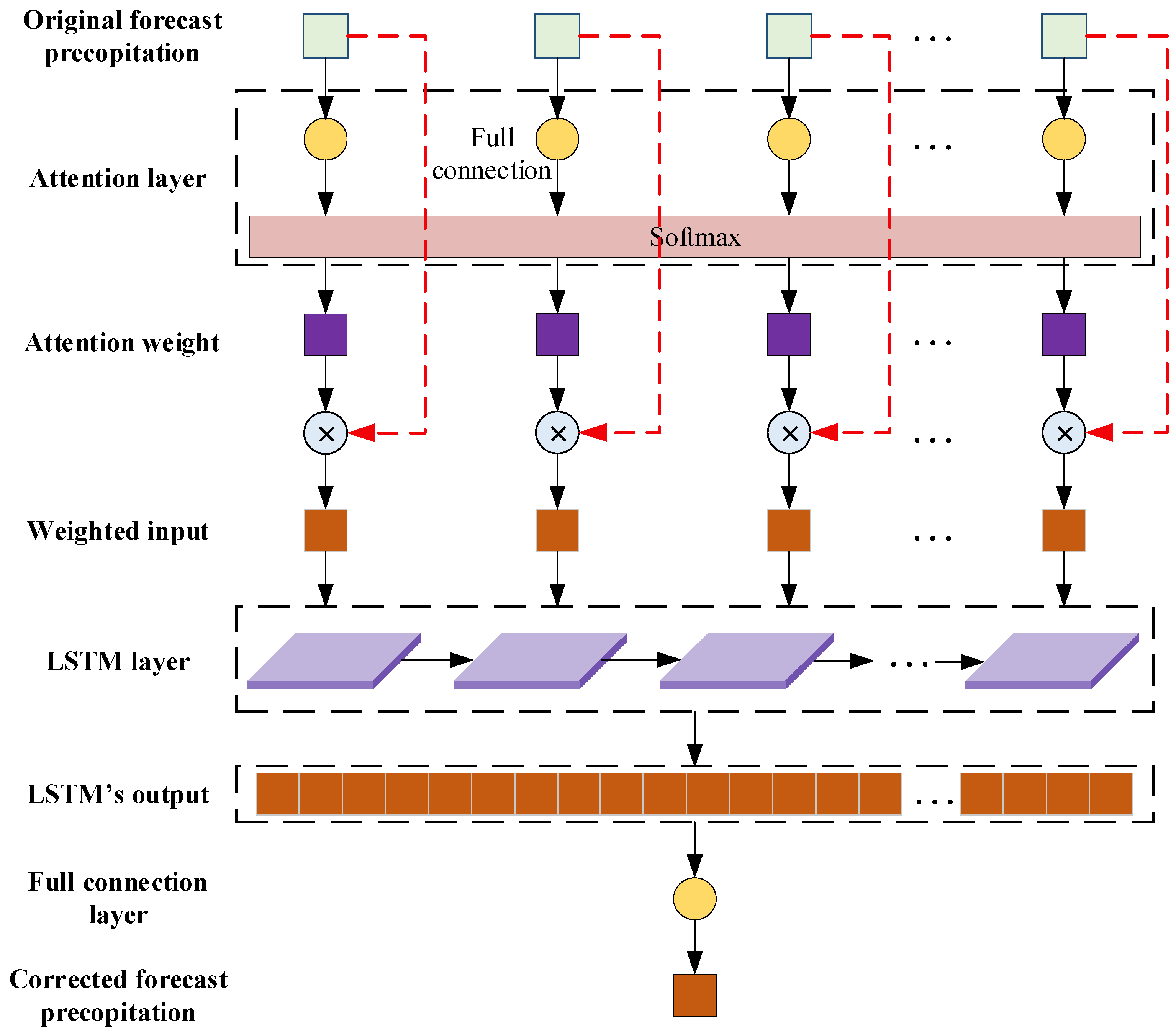
3.3.3. LSTM-A
3.3.4. A-LSTM
3.4. Performance Evaluation
3.4.1. Accuracy Evaluation of Integrated Forecast Precipitation
3.4.2. Applicability Testing of Integrated Forecast Precipitation
4. Results and Discussion
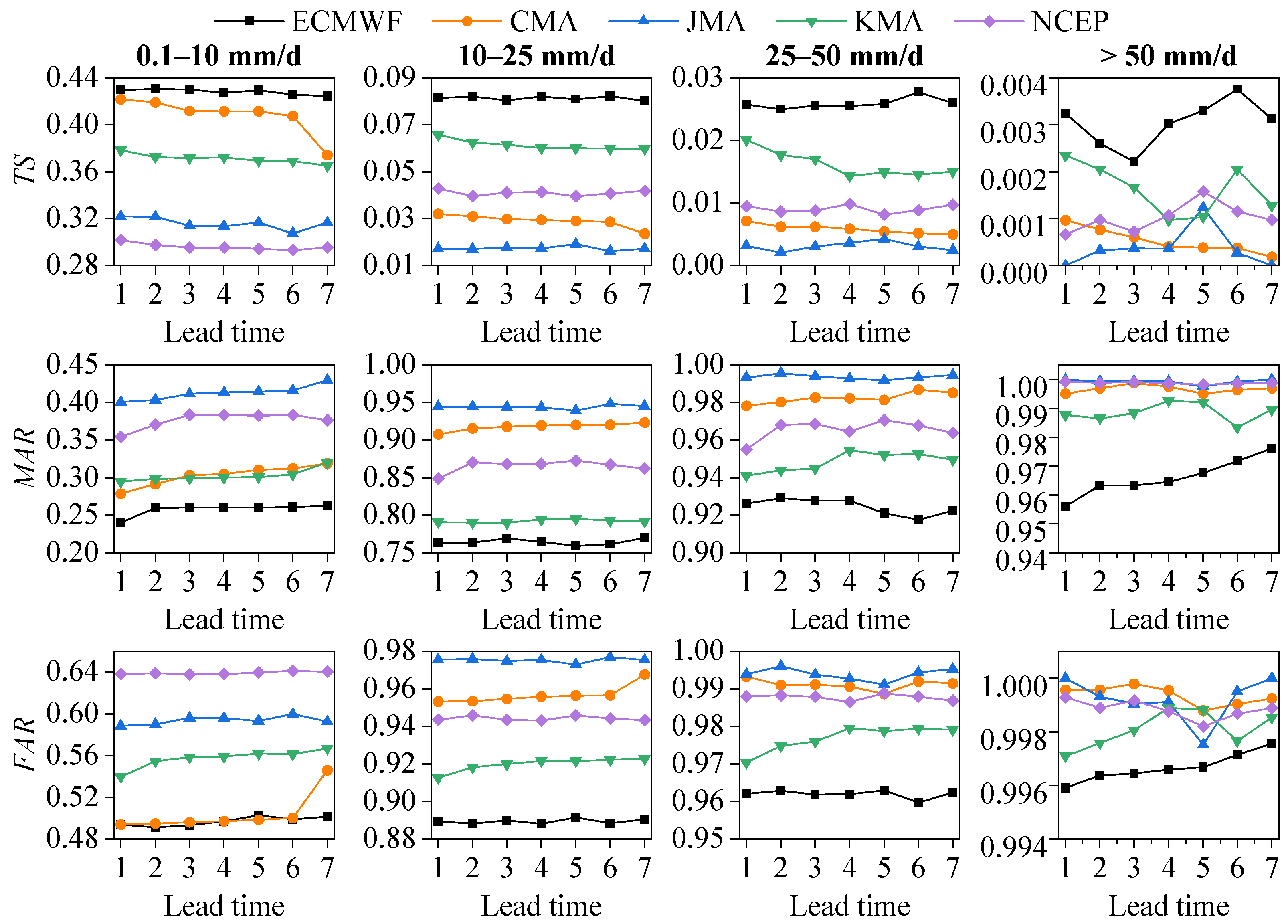
4.1. Accuracy Evaluation of Original Forecast Precipitation Under Different Lead Times
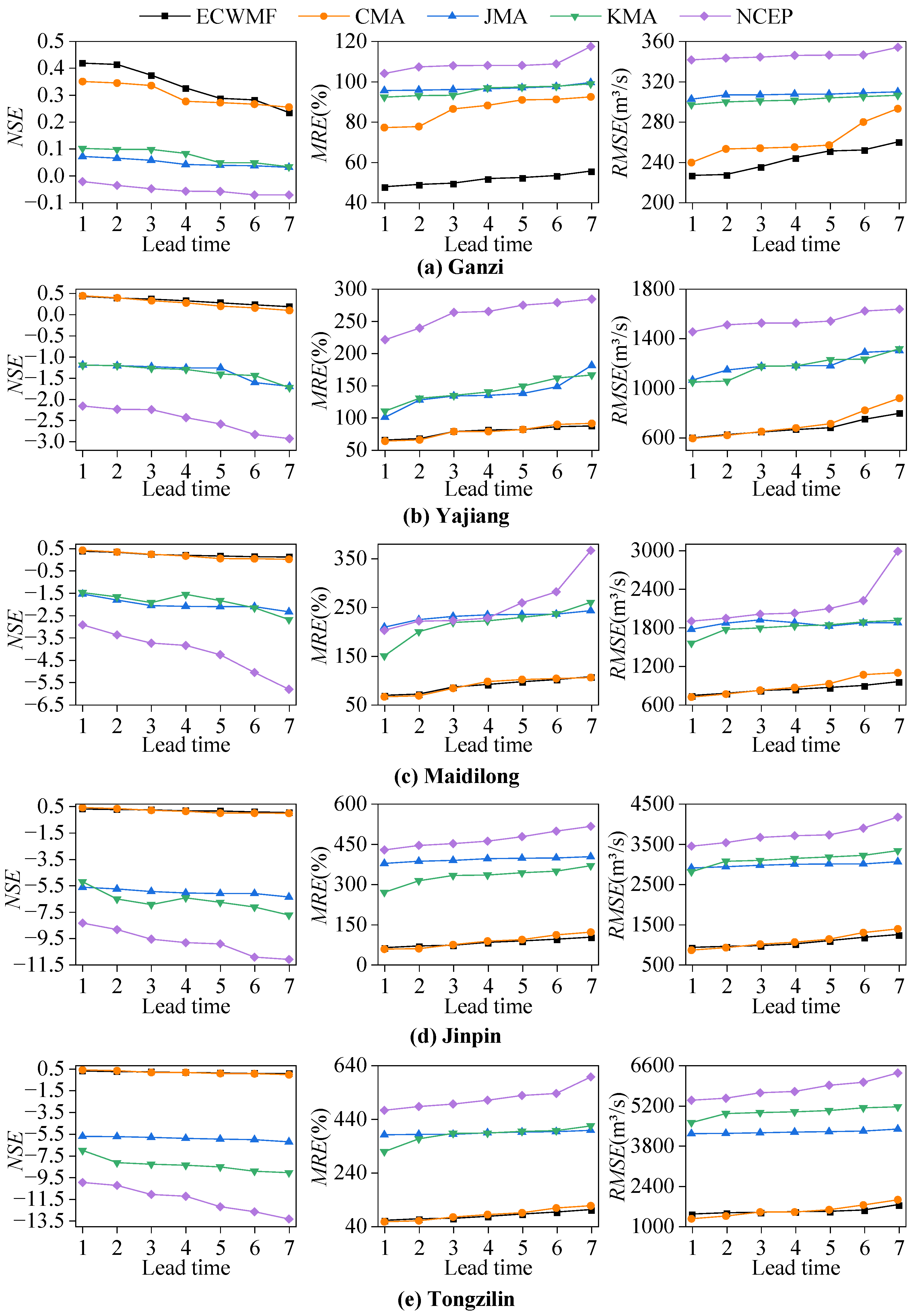
4.2. Applicability Evaluation of Original Forecast Precipitation
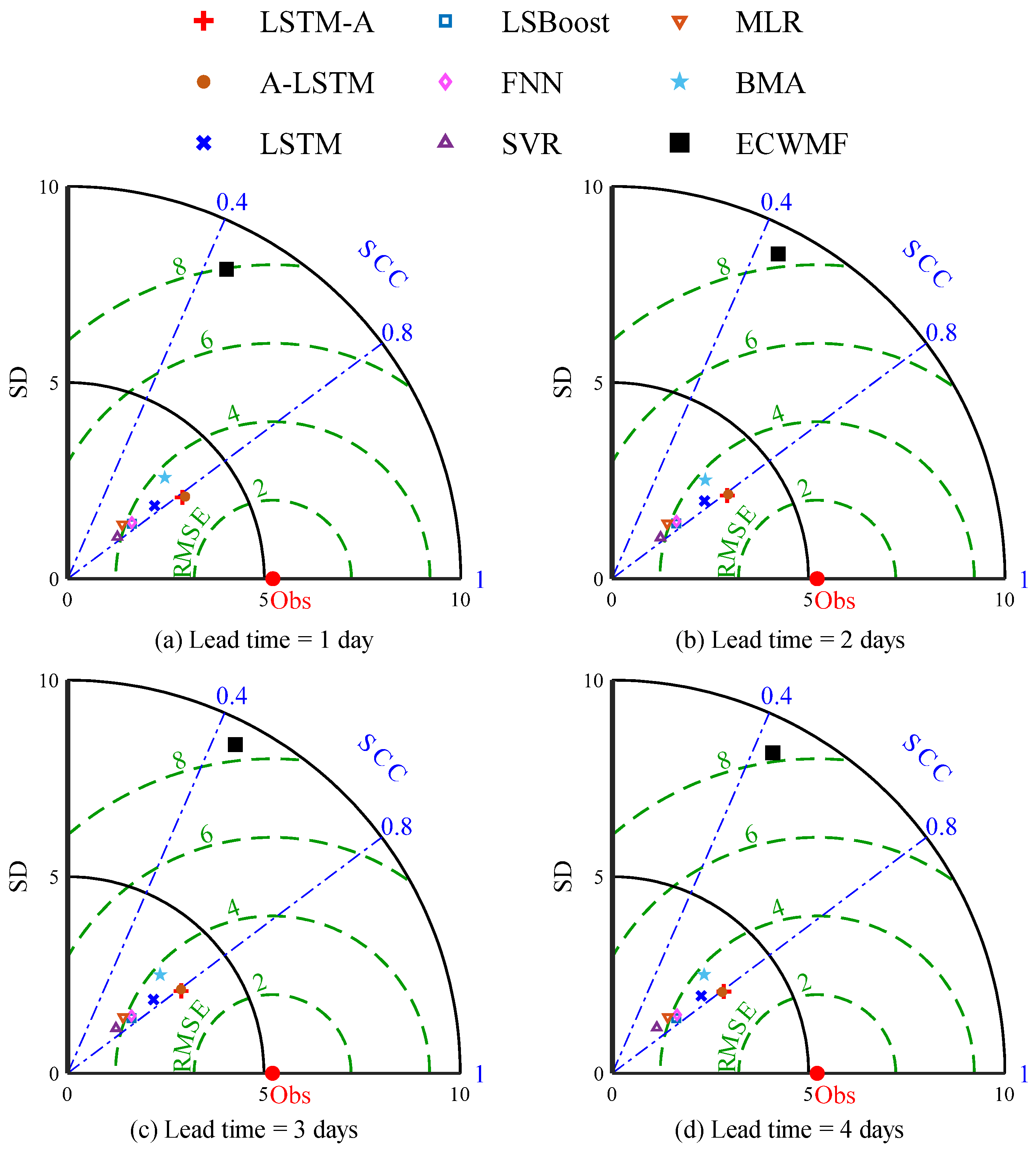
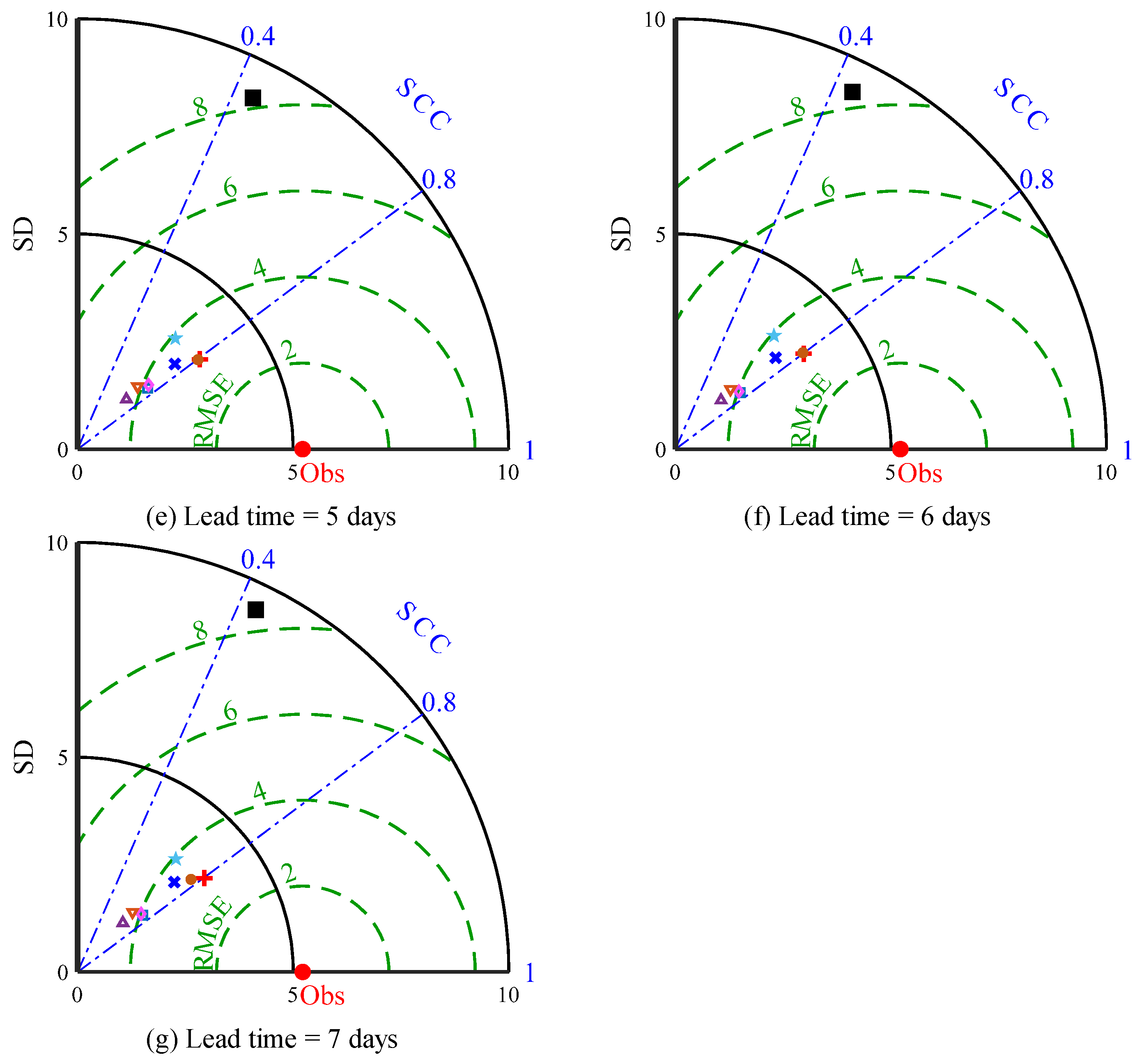
4.3. Comparison of Integrated Forecast Precipitation Accuracy for Different Models
4.4. Applicability Testing for Integrated Forecast Precipitation
5. Conclusions
- (1)
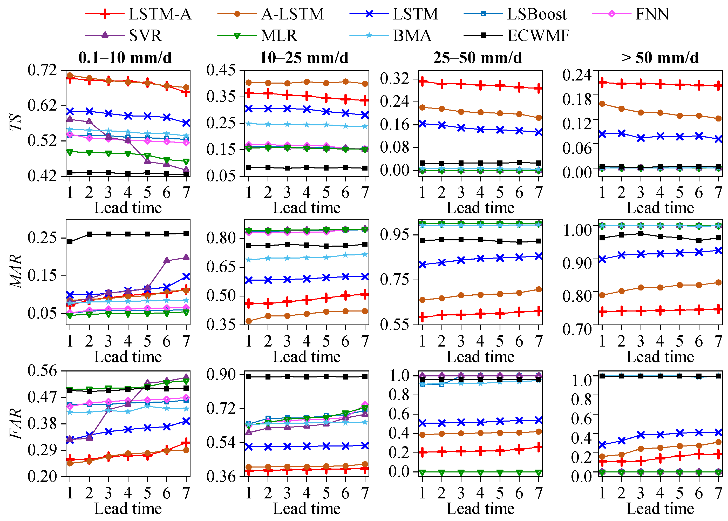
- Among five original forecast precipitation models, the ECMWF and CMA had a higher forecast precipitation accuracy under different intensities and a better applicability in streamflow forecast, but they all failed to forecast precipitation of a ≥10 mm/d intensity under different lead times well.
- (2)
- General machine learning models (LSBoost, FNN, SVR, MLR, and BMA) were unable to adequately learn the fluctuation of precipitation sequences, and lost the ability to forecast precipitation of a ≥25 mm/d intensity because they tended to sacrifice the ability to fit high values during internal training to maintain their overall accuracy.
- (3)
- Among the integration models, LSTM-A and A-LSTM had the best performance and effectively reduced precipitation forecast errors under different intensities, indicating that deep learning with a strong temporal feature capture ability significantly improves precipitation forecast accuracy.
- (4)
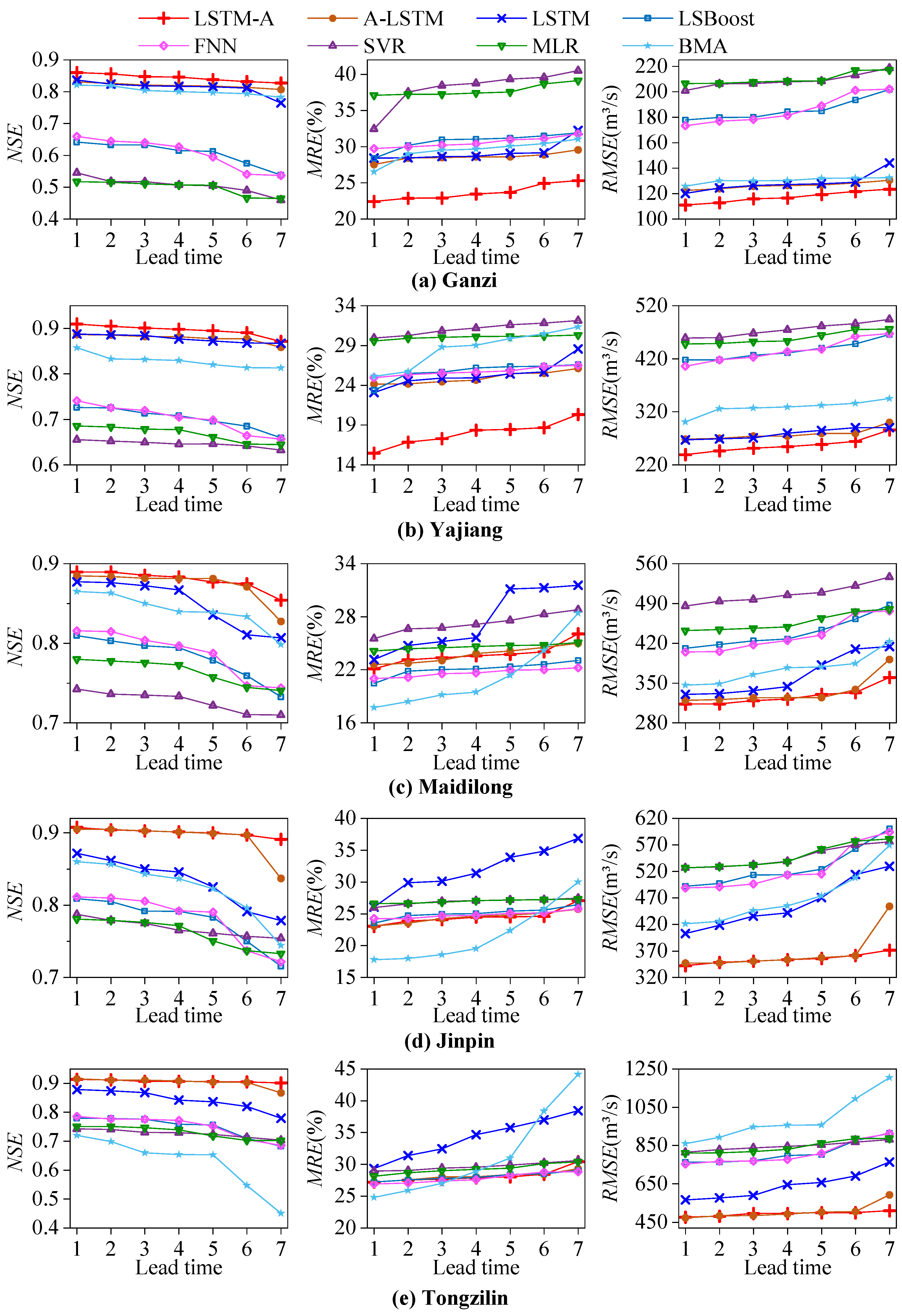
- Regarding the applicability of forecast precipitation in streamflow forecast, LSTM-A was the best, with an NSE above 0.82 and MRE below 30% at each hydrologic station under different lead times, which can be directly applied in real-time streamflow forecast.
Author Contributions
Funding
Data Availability Statement
Acknowledgments
Conflicts of Interest
References
- Chen, Y.; Li, D.; Zhao, Q.; Cai, X. Developing a Generic Data-Driven Reservoir Operation Model. Adv. Water Resour. 2022, 167, 104274. [Google Scholar] [CrossRef]
- Meng, J.; Dong, Z.; Fu, G.; Zhu, S.; Shao, Y.; Wu, S.; Li, Z. Spatial and Temporal Evolution of Precipitation in the Bahr El Ghazal River Basin, Africa. Remote Sens. 2024, 16, 1638. [Google Scholar] [CrossRef]
- Chen, H.; Zhang, H.; Jang, S.G.; Liu, X.; Xing, L.; Wu, Z.; Zhang, L.; Liu, Y.; Chen, C. Road Criticality Assessment to Improve Commutes during Floods. J. Environ. Manag. 2024, 349, 119592. [Google Scholar] [CrossRef] [PubMed]
- Zhu, S.; Huang, W.; Luo, X.; Guo, J.; Yuan, Z. The Spread of Multiple Droughts in Different Seasons and Its Dynamic Changes. Remote Sens. 2023, 15, 3848. [Google Scholar] [CrossRef]
- Yan, L.; Zhang, L.; Xiong, L.; Yan, P.; Jiang, C.; Xu, W.; Xiong, B. Flood Frequency Analysis Using Mixture Distributions in Light of Prior Flood Type Classification in Norway. Remote Sens. 2023, 15, 401. [Google Scholar] [CrossRef]
- Compilation group of China Flood and Drought Disaster Prevention Bulletin. Summary of China Flood and Drought Disaster Prevention Bulletin 2022. China Flood Drought Manag. 2023, 33, 78–82. [Google Scholar] [CrossRef]
- Na, W.; Yoo, C. Real-Time Bias Correction of Rainfall Nowcasts Using Biward Tracking Method. J. Hydrol. 2023, 622, 129642. [Google Scholar] [CrossRef]
- Zhou, K.; Sun, J.; Zheng, Y.; Zhang, Y. Quantitative Precipitation Forecast Experiment Based on Basic NWP Variables Using Deep Learning. Adv. Atmos. Sci. 2022, 39, 1472–1486. [Google Scholar] [CrossRef]
- Liu, J.; Qiu, Q.; Li, C.; Jiao, Y.; Wang, W.; Fuliang, Y. Advances of Precipitation Nowcasting and Its Application in Hydrological Forecasting. Adv. Water Sci. 2020, 31, 129–142. [Google Scholar]
- Ayzel, G.; Scheffer, T.; Heistermann, M. RainNet v1.0: A Convolutional Neural Network for Radar-Based Precipitation Nowcasting. Geosci. Model Dev. 2020, 13, 2631–2644. [Google Scholar] [CrossRef]
- Aminyavari, S.; Saghafian, B.; Delavar, M. Evaluation of TIGGE Ensemble Forecasts of Precipitation in Distinct Climate Regions in Iran. Adv. Atmos. Sci. 2018, 35, 457–468. [Google Scholar] [CrossRef]
- Li, X.; Wei, Z.; Ma, L. Prediction Abilities of Subseasonal-to-Seasonal Models for Regional Rainstorm Processes in South China. Int. J. Climatol. 2023, 43, 2896–2912. [Google Scholar] [CrossRef]
- Zhou, C.; Zhao, P.; Liu, G.; Xiao, A.; Yu, H. Decadal Difference in Influential Factors for Interannual Variations of Winter Tibetan Plateau Snow. Atmos. Res. 2023, 288, 106718. [Google Scholar] [CrossRef]
- Zhuo, W.; Huang, J.; Gao, X.; Ma, H.; Huang, H.; Su, W.; Meng, J.; Li, Y.; Chen, H.; Yin, D. Prediction of Winter Wheat Maturity Dates through Assimilating Remotely Sensed Leaf Area Index into Crop Growth Model. Remote Sens. 2020, 12, 2896. [Google Scholar] [CrossRef]
- Luo, C.; Xiao, F.; Gong, L.; Lei, J.; Li, W.; Zhang, S. Comparison of Weighted Mean Temperature in Greenland Calculated by Four Reanalysis Data. Remote Sens. 2022, 14, 5431. [Google Scholar] [CrossRef]
- Cong, J.; Wu, Z.; Ma, Y.; Xu, S.; Wang, Y.; Sun, M.; Nie, C. Improving Numerical Forecast of the Rainstorms Induced by Mongolia Cold Vortex in North China with the Frequency Matching Method. Atmos. Res. 2021, 262, 105791. [Google Scholar] [CrossRef]
- Jiang, X.; Zhang, L.; Liang, Z.; Fu, X.; Wang, J.; Xu, J.; Zhang, Y.; Zhong, Q. Study of Early Flood Warning Based on Postprocessed Predicted Precipitation and Xinanjiang Model. Weather Clim. Extrem. 2023, 42, 100611. [Google Scholar] [CrossRef]
- Yang, C.; Yuan, H.; Su, X. Bias Correction of Ensemble Precipitation Forecasts in the Improvement of Summer Streamflow Prediction Skill. J. Hydrol. 2020, 588, 124955. [Google Scholar] [CrossRef]
- Su, X.; Yuan, H.; Zhu, Y. A Comparative Study of Four Objective Quantitative Precipitation Forecast Calibration Methods. Acta Meteorol. Sin. 2021, 79, 132–149. [Google Scholar] [CrossRef]
- Zhuang, X. Study on Revised Forecast Method of Station Precipitation Based on Error Weight. Meteorol. Disaster Reduct. Res. 2022, 45, 196–206. [Google Scholar]
- Tang, X.; Zhou, R.; He, X.; Wang, J.; Ren, X. Research on Application of Multi-Source Precipitation Forecast Integration Technology. J. Meteorol. Environ. 2021, 37, 26–32. [Google Scholar]
- Liu, Q.; Lou, X.; Yan, Z.; Qi, Y.; Jin, Y.; Yu, S.; Yang, X.; Zhao, D.; Xia, J. Deep-Learning Post-Processing of Short-Term Station Precipitation Based on NWP Forecasts. Atmos. Res. 2023, 295, 107032. [Google Scholar] [CrossRef]
- Liu, X.; Zhang, L.; She, D.; Chen, J.; Xia, J.; Chen, X.; Zhao, T. Postprocessing of Hydrometeorological Ensemble Forecasts Based on Multisource Precipitation in Ganjiang River Basin, China. J. Hydrol. 2022, 605, 127323. [Google Scholar] [CrossRef]
- Tang, Y.; Wu, Q.; Soomro, S.; Li, X.; Sun, Y.; Hu, C. Comparison of Different Ensemble Precipitation Forecast System Evaluation, Integration and Hydrological Applications. Acta Geophys. 2023, 71, 405–421. [Google Scholar] [CrossRef]
- Wu, J.; Lu, G.; Wu, Z. Flood Forecasts Based on Multi-Model Ensemble Precipitation Forecasting Using a Coupled Atmospheric-Hydrological Modeling System. Nat. Hazards 2014, 74, 325–340. [Google Scholar] [CrossRef]
- Zhi, X.; Zhao, C. Heavy Precipitation Forecasts Based on Multi-Model Ensemble Members. J. Appl. Meteorol. Sci. 2020, 31, 303–314. [Google Scholar]
- Zhang, Y.; Ye, A. Machine Learning for Precipitation Forecasts Postprocessing: Multimodel Comparison and Experimental Investigation. J. Hydrometeorol. 2021, 22, 3065–3085. [Google Scholar] [CrossRef]
- Moradian, S.; AghaKouchak, A.; Gharbia, S.; Broderick, C.; Olbert, A.I. Forecasting of Compound Ocean-Fluvial Floods Using Machine Learning. J. Environ. Manag. 2024, 364, 121295. [Google Scholar] [CrossRef]
- Zhu, W.; Sheng, C.; Fan, S.; Rong, Y.; Qu, M. Research on Multi-Model Integrated Precipitation Forecast Based on Feed Forward Neural Network. J. Arid Meteorol. 2024, 42, 117–128. [Google Scholar]
- Wang, Y.; Peng, L.; Yang, L.E.; Wang, Z.; Deng, X. Attributing Effects of Classified Infrastructure Management on Mitigating Urban Flood Risks: A Case Study in Beijing, China. Sustain. Cities Soc. 2024, 101, 105141. [Google Scholar] [CrossRef]
- Yan, R.; Liu, L.; Liu, W.; Wu, S. Quantitative Flood Disaster Loss-Resilience with the Multilevel Hybrid Evaluation Model. J. Environ. Manag. 2023, 347, 119026. [Google Scholar] [CrossRef] [PubMed]
- Fang, W.; Qin, H.; Liu, G.; Yang, X.; Xu, Z.; Jia, B.; Zhang, Q. A Method for Spatiotemporally Merging Multi-Source Precipitation Based on Deep Learning. Remote Sens. 2023, 15, 4160. [Google Scholar] [CrossRef]
- Gebrechorkos, S.H.; Pan, M.; Beck, H.E.; Sheffield, J. Performance of State-of-the-Art C3S European Seasonal Climate Forecast Models for Mean and Extreme Precipitation Over Africa. Water Resour. Res. 2022, 58, e2021WR031480. [Google Scholar] [CrossRef]
- Heidari, A.; Navimipour, N.J.; Unal, M. Applications of ML/DL in the Management of Smart Cities and Societies Based on New Trends in Information Technologies: A Systematic Literature Review. Sustain. Cities Soc. 2022, 85, 104089. [Google Scholar] [CrossRef]
- Li, Y.; Tong, Z.; Tong, S.; Westerdahl, D. A Data-Driven Interval Forecasting Model for Building Energy Prediction Using Attention-Based LSTM and Fuzzy Information Granulation. Sustain. Cities Soc. 2022, 76, 103481. [Google Scholar] [CrossRef]
- Jahani, A.; Zare, K.; Mohammad Khanli, L. Short-Term Load Forecasting for Microgrid Energy Management System Using Hybrid SPM-LSTM. Sustain. Cities Soc. 2023, 98, 104775. [Google Scholar] [CrossRef]
- Zhang, Z.; Qin, H.; Li, J.; Liu, Y.; Yao, L.; Wang, Y.; Wang, C.; Pei, S.; Li, P.; Zhou, J. Operation Rule Extraction Based on Deep Learning Model with Attention Mechanism for Wind-Solar-Hydro Hybrid System under Multiple Uncertainties. Renew. Energy 2021, 170, 92–106. [Google Scholar] [CrossRef]
- Guo, M.H.; Xu, T.X.; Liu, J.J.; Liu, Z.N.; Jiang, P.T.; Mu, T.J.; Zhang, S.H.; Martin, R.R.; Cheng, M.M.; Hu, S.M. Attention Mechanisms in Computer Vision: A Survey. Comput. Vis. Media 2022, 8, 331–368. [Google Scholar] [CrossRef]
- Ma, X.; Ji, S.; Wang, J.; Liu, X.; Wang, H. Classification of Hyperspectral Image Based on Task-Specific Learning Network. IEEE Trans. Geosci. Remote Sens. 2021, 59, 8646–8656. [Google Scholar] [CrossRef]
- Fang, W.; Qin, H.; Shen, K.; Yang, X.; Yang, Y.; Jia, B. Extracting Operation Rule of Cascade Reservoirs Using a Novel Framework Considering Hydrometeorological Spatiotemporal Information Based on Artificial Intelligence Models. J. Clean. Prod. 2024, 437, 140608. [Google Scholar] [CrossRef]
- Xiong, L.; Liu, C.; Chen, S.; Zha, X.; Ma, Q. Review of Post-Processing Research for Remote-Sensing Precipitation Products. Adv. Water Resour. 2021, 32, 627–637. [Google Scholar]
- Jahangir, M.S.; Quilty, J. Temporal Hierarchical Reconciliation for Consistent Water Resources Forecasting across Multiple Timescales: An Application to Precipitation Forecasting. Water Resour. Res. 2022, 58, e2021WR031862. [Google Scholar] [CrossRef]
- Jiang, M.; Weng, B.; Chen, J.; Huang, T.; Ye, F.; You, L. Transformer-Enhanced Spatiotemporal Neural Network for Post-Processing of Precipitation Forecasts. J. Hydrol. 2024, 630, 130720. [Google Scholar] [CrossRef]
- Lang, S.T.K.; Dawson, A.; Diamantakis, M.; Dueben, P.; Hatfield, S.; Leutbecher, M.; Palmer, T.; Prates, F.; Roberts, C.D.; Sandu, I.; et al. More Accuracy with Less Precision. Q. J. R. Meteorol. Soc. 2021, 147, 4358–4370. [Google Scholar] [CrossRef]
- Morales, A.; Posselt, D.J.; Morrison, H.; He, F. Assessing the Influence of Microphysical and Environmental Parameter Perturbations on Orographic Precipitation. J. Atmos. Sci. 2019, 76, 1373–1395. [Google Scholar] [CrossRef]
- Purr, C.; Brisson, E.; Schlünzen, K.H.; Ahrens, B. Convective Rain Cell Properties and the Resulting Precipitation Scaling in a Warm-Temperate Climate. Q. J. R. Meteorol. Soc. 2022, 148, 1768–1781. [Google Scholar] [CrossRef]


| Hydrologic Station | Calibration Period | Validation Period | ||||
|---|---|---|---|---|---|---|
| NSE | MRE (%) | RMSE (m3/s) | NSE | MRE (%) | RMSE (m3/s) | |
| Ganzi | 0.872 | 17.5 | 106 | 0.867 | 18.3 | 112 |
| Yajiang | 0.972 | 10.2 | 142 | 0.961 | 12.5 | 158 |
| Maidilong | 0.982 | 3.9 | 132 | 0.980 | 4.3 | 135 |
| Jinpin | 0.985 | 5.9 | 141 | 0.983 | 6.5 | 145 |
| Tongzilin | 0.983 | 9.2 | 227 | 0.979 | 9.8 | 234 |
| Lead Time (Day) | 1 | 2 | 3 | 4 | 5 | 6 | 7 | |
|---|---|---|---|---|---|---|---|---|
| Model | ||||||||
| LSTM-A | 1.56 | 1.57 | 1.59 | 1.61 | 1.61 | 1.64 | 1.75 | |
| A-LSTM | 1.60 | 1.61 | 1.65 | 1.65 | 1.67 | 1.67 | 1.70 | |
| LSTM | 1.60 | 1.62 | 1.65 | 1.66 | 1.69 | 1.70 | 1.70 | |
| LSBoost | 2.16 | 2.17 | 2.17 | 2.17 | 2.18 | 2.19 | 2.20 | |
| FNN | 2.18 | 2.18 | 2.20 | 2.20 | 2.21 | 2.22 | 2.23 | |
| SVR | 1.85 | 1.86 | 1.95 | 2.02 | 2.09 | 2.09 | 2.19 | |
| MLR | 2.25 | 2.25 | 2.26 | 2.26 | 2.27 | 2.29 | 2.30 | |
| BMA | 2.68 | 2.69 | 2.71 | 2.72 | 2.82 | 2.83 | 2.84 | |
| ECMWF | 4.26 | 4.20 | 4.19 | 4.20 | 4.32 | 4.29 | 4.30 | |
Disclaimer/Publisher’s Note: The statements, opinions and data contained in all publications are solely those of the individual author(s) and contributor(s) and not of MDPI and/or the editor(s). MDPI and/or the editor(s) disclaim responsibility for any injury to people or property resulting from any ideas, methods, instructions or products referred to in the content. |
© 2024 by the authors. Licensee MDPI, Basel, Switzerland. This article is an open access article distributed under the terms and conditions of the Creative Commons Attribution (CC BY) license (https://creativecommons.org/licenses/by/4.0/).
Share and Cite
Fang, W.; Qin, H.; Lin, Q.; Jia, B.; Yang, Y.; Shen, K. Deep Learning Integration of Multi-Model Forecast Precipitation Considering Long Lead Times. Remote Sens. 2024, 16, 4489. https://doi.org/10.3390/rs16234489
Fang W, Qin H, Lin Q, Jia B, Yang Y, Shen K. Deep Learning Integration of Multi-Model Forecast Precipitation Considering Long Lead Times. Remote Sensing. 2024; 16(23):4489. https://doi.org/10.3390/rs16234489
Chicago/Turabian StyleFang, Wei, Hui Qin, Qian Lin, Benjun Jia, Yuqi Yang, and Keyan Shen. 2024. "Deep Learning Integration of Multi-Model Forecast Precipitation Considering Long Lead Times" Remote Sensing 16, no. 23: 4489. https://doi.org/10.3390/rs16234489
APA StyleFang, W., Qin, H., Lin, Q., Jia, B., Yang, Y., & Shen, K. (2024). Deep Learning Integration of Multi-Model Forecast Precipitation Considering Long Lead Times. Remote Sensing, 16(23), 4489. https://doi.org/10.3390/rs16234489