Self-Activated Implicit Neural Representation for Synthetic Aperture Radar Images

Abstract

Image Implicit Neural Representations (INRs) adopt a neural network to learn a continuous function for mapping the pixel coordinates to their corresponding values. This task has gained significant attention for representing images in a continuous manner. Despite substantial progress regarding natural images, there is little investigation of INRs for Synthetic Aperture Radar (SAR) images. This work takes a pioneering effort to study INRs for SAR images and finds that fine details are hard to represent. It has been shown in prior works that fine details can be easier to learn when the model weights are better initialized, which motivated us to investigate the benefits of activating the model weight before target training. The challenge of this task lies in the fact that SAR images cannot be used during the model activation stage. To this end, we propose exploiting a cross-pixel relationship of the model output, which relies on no target images. Specifically, we design a novel self-activation method by alternatively using two loss functions: a loss used to smooth out the model output, and another used for the opposite purpose. Extensive results on SAR images empirically show that our proposed method helps improve the model performance by a non-trivial margin.

1. Introduction

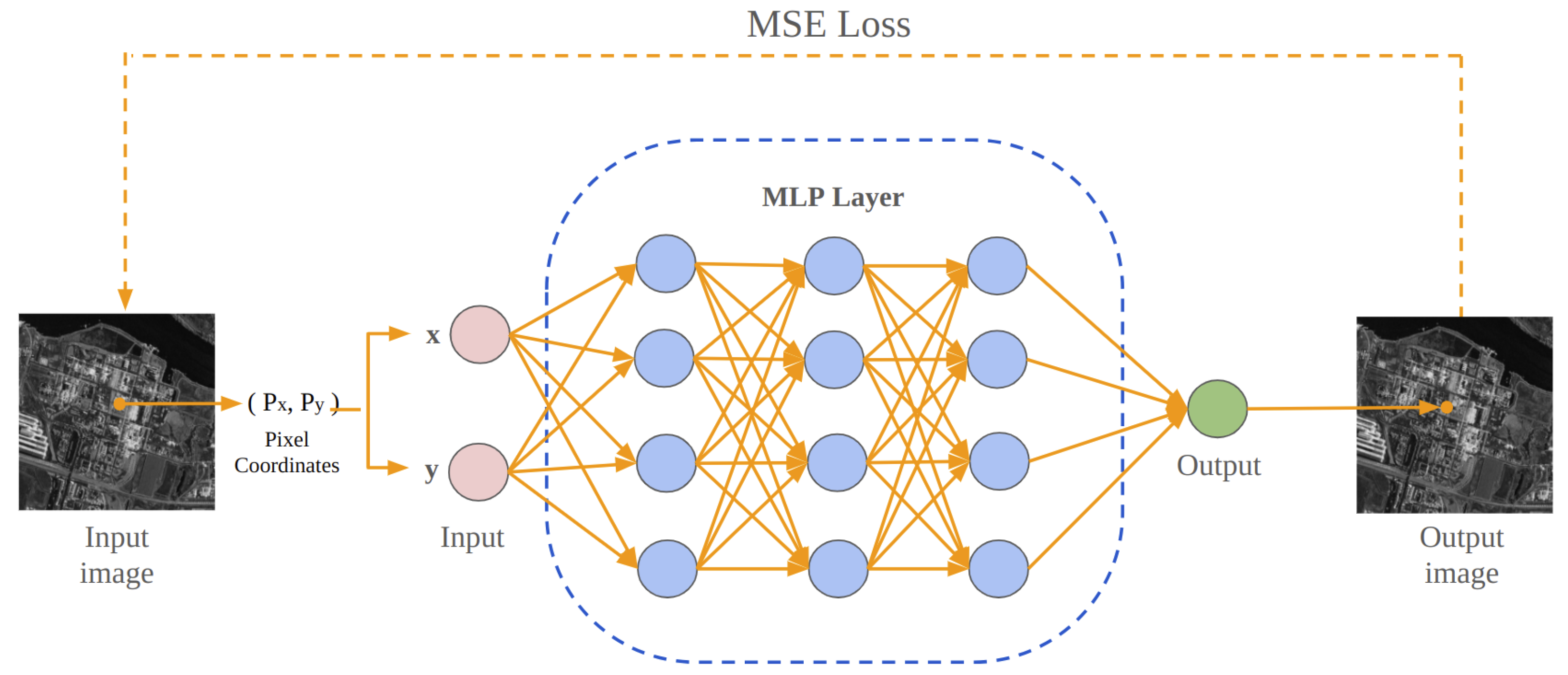
Implicit Neural Representations (INRs) are a novel area of research that can continuously represent a signal, in contrast to traditional discrete representations, such as images represented by grid-sampled discrete pixels [1]. The core concept of INRs is to employ Multi-Layer Perceptron (MLP) networks to learn the implicit parameterization of continuous functions [2]. For example, given a 2D image, the network learns a continuous function that relates pixel coordinates to pixel values, using the pixel coordinates $x\in {\mathbb{R}}^2$ as input to train the network to output the corresponding values ($y\in {\mathbb{R}}^3$ for RGB and $y\in \mathbb{R}$ for grayscale) [3]. Based on the capability of INRs to express continuous functions, their recent success in various applications, such as surface representation, volume rendering, and image compression, highlights INRs’ versatility and effectiveness in modern computational tasks [4]. To enhance the model’s ability to learn and represent signals, prior works have utilized different activation functions and initialization methods for the INR model [5], demonstrating that suitable initialization techniques can significantly improve the model’s capacity to capture high-frequency information.

Synthetic Aperture Radar (SAR) is a system that achieves high-resolution ground imaging through radar technology [6,7]. Its working principle involves emitting pulse electromagnetic waves and receiving the signals reflected from the surface of the target to obtain reflection information [8,9]. Compared to traditional optical imaging technologies, SAR can function effectively even under extreme weather conditions, such as fog or rain [10], demonstrating greater stability and resistance to interference [11]. This makes it widely applicable in areas such as remote sensing, military reconnaissance, and geological exploration [12]. However, for high-precision imaging tasks, SAR often requires the fusion of data from multiple perspectives or different radar frequencies, which poses challenges for traditional deep-learning methods, particularly in terms of generalization ability and the accurate capture of high-frequency features [13]. Due to the unique noise characteristics and imaging mechanism of SAR images, many studies have attempted to use neural networks with various techniques for tasks such as object detection [14] and image denoising [15,16] on SAR images, achieving significant progress in these areas.

An image signal, such as an SAR image, is essentially a discrete signal made up of a finite set of coordinates and their corresponding pixel values, which represents the conventional method of expressing images. In contrast to this conventional representation, INR offers a new continuous representation with the following advantages. Firstly, compared to traditional methods, INR decouples the image signal from the number of discrete pixels, allowing for sampling at arbitrary spatial resolutions and providing what can be described as different resolutions. Secondly, as INR is based on neural networks for signal representation, the memory requirements are independent of spatial resolution and are closely related to the neural network itself. Extensive research has examined continuous representations of various image types, including natural images [17], hyperspectral images [18], and CT images [19]. However, despite the widespread use of SAR images across various tasks, their continuous representations have not yet been explored through INR. This work pioneers the use of INRs for SAR images to address this gap.

In our preliminary investigation, we find that directly applying existing INR methods to represent SAR images poses challenges in capturing fine details. Based on previous research [17,20,21], proper model weight initialization is essential in learning INR and plays a decisive role in the model’s capability to capture signal details. Inspired by the effectiveness of weight initialization in improving model performance, we explore the possibility of activating the model weights before target training. However, the challenge with activating model weights is that the information from the target image cannot be utilized at this stage. Consequently, we propose a self-activation method that utilizes the loss function on the model output to activate the model weights by exploiting the cross-pixel relationships within the model output.

The loss function used in our self-activation method comprises two opposing components: anti-smoothness sub-loss and smoothness sub-loss, both of which adjust the cross-pixel relationships of the model’s original output through image gradients before learning the target image. Specifically, the smoothness loss reduces the output image gradient, decreasing the differences between neighboring pixels and smoothing the output. In contrast, the anti-smoothness loss increases the output image gradient, enhancing the differences between neighboring pixels, which makes the output coarse. By alternately adjusting the model’s output with two opposing loss functions, the goal of activating the INR model is achieved. We demonstrate that the shift-invariance of the INR model’s Neural Tangent Kernel (NTK) can be enhanced through our model’s self-activation method, significantly improving its ability to capture high-frequency components and its overall representational capacity. Extensive experimental results demonstrate that self-activating the INR model with the two proposed opposing loss functions can significantly enhance its performance in representing SAR images.

Overall, our contributions are summarized as follows:

• We investigate learning INR for SAR images and find that activating model weights before training can facilitate the model capture of fine details.
• We propose a self-activation method to initialize the INR model weights, which does not require any information from the target image as input.
• We conduct extensive experiments on SAR images, demonstrating that our proposed self-activation method improves model performance by a non-trivial margin.

2. Related Work

2.1. Implict Neural Representation

Implicit Neural Representations (INRs) achieve compact and efficient representations of complex signals by directly mapping coordinates to signal values through neural networks, such as Multi-Layer Perceptrons (MLPs). Compared to traditional signal representation methods [22,23,24], INRs offer greater flexibility and precision through continuous mappings and have been widely applied to various complex signal processing tasks, including image super-resolution [25], view synthesis [26], and three-dimensional reconstruction [27]. In recent years, numerous studies have emerged to optimize INR performance, particularly in terms of reconstruction speed and accuracy. SIREN [20] introduces sine functions as activation functions and uses a specific weight initialization strategy, significantly enhancing the model’s ability to represent fine details of continuous signals. DINER [28] introduces an order-invariant INR model, demonstrating enhanced robustness when handling noisy or unordered data. FINER [17] is based on SIREN and proposes variable-periodic activation functions and explores a modified model weight initialization to address the frequency tuning limitations in INR technology. WIRE [21] incorporates Gabor wavelet activation functions and employs an optimized initialization strategy, improving the accuracy of signal reconstruction. These advancements have not only promoted the widespread application of INRs in image and audio reconstruction but have also expanded their potential in fields such as medical imaging [19], three-dimensional scene reconstruction [29], and computer vision [30]. Overall, the various INR models explore different methods to represent the fine details of the target signal and demonstrate the importance of model weight initialization for signal representation in INR models. We explore the possibility of activating the INR model prior to training and utilizing a self-activation method to initialize the model weights, enabling the model to capture fine details in SAR images.

2.2. Synthetic Aperture Radar Image

Synthetic Aperture Radar (SAR) is an active remote sensing technology that can produce high-resolution images even under adverse weather conditions. By emitting microwave signals and capturing their reflections, SAR generates detailed images of the Earth’s surface. It is widely applied in areas such as disaster response [31], environmental monitoring [32], urban planning [33], and military applications [34]. In research, commonly used SAR datasets include MSTAR [35], a benchmark for target recognition studies. This dataset features SAR images of various military targets, such as tanks and trucks, captured from different angles and imaging conditions. Another significant dataset is TerraSAR-X [36], which offers images with resolutions of up to one meter across various scenes—from urban areas to oceans—supporting a broad range of research and applications. Previous studies on SAR image processing have seen Convolutional Neural Networks (CNNs) demonstrate reliability in solving image recognition tasks [37]. Autoencoders [38] have been effective in removing speckle noise from SAR images while retaining key structural information. Generative Adversarial Networks (GANs) [39] have excelled in SAR image super-resolution tasks. Meanwhile, attention mechanisms [40] have been widely used in target detection and image classification. Multi-stream networks [41], capable of integrating multi-source input data, are extensively utilized in multimodal data fusion and the analysis of SAR images in complex scenes. Long Short-Term Memory (LSTM) networks [42] have unique applications in processing the sequences of SAR images generated over multiple time points. While existing research has greatly expanded the possibilities for SAR image processing, challenges like signal complexity and speckle noise continue to affect SAR image reconstruction methods. Given the widespread application of SAR images, we pioneeringly explore the possibility of utilizing the INR model for the continuous representation of SAR images and employ an activation method before training to enhance the model’s capability to represent SAR images.

3. Background and Method

Formulation of INR. Implicit Neural Representations (INRs) have garnered significant attention for their ability to continuously represent signals and have been applied to computer vision tasks such as image generation [43], novel view synthesis [44], and 3D reconstruction [45], exhibiting remarkable visual performance. Specifically, INR provides a novel approach to parameterizing signals, using continuous functions to map signal domains to attribute values at each coordinate, in contrast to traditional, typically discrete signal representations. By inputting continuous spatial coordinates such as image coordinates, or 3D space coordinates, Implicit Neural Representations (INRs) predict the corresponding output signal values, which can include pixel values or signal amplitudes. We utilize a Multi-Layer Perceptron (MLP) [46] as an INR function model, $f_{\psi }$, to perform the mapping:

$$f_{\psi }:{\mathbb{R}}^{D_{\mathrm{in}}}\to {\mathbb{R}}^{D_{\mathrm{out}}}$$

(1)

This mapping enables the transformation of input dimensions, $D_{\mathrm{in}}$, which represent the spatial coordinates, into output dimensions, $D_{\mathrm{out}}$, which represent the predicted pixel values or signal amplitudes. In this context, $\psi$ denotes the learnable parameters of the network MLP. By optimizing $\psi$, the MLP gradually approximates the target function, $T\left(x\right)\approx f_{\psi }$, by multi-layer, which can be formulated as follows,

$$f_{\psi }\left(x\right)=\sigma (W_n{x}_{n-1}+b_n),$$

(2)

where $y_n$ is the output of the hidden layer in the n-th layer of the MLP, $\sigma$ is the nonlinear activation function, and $W_n$ and $b_n$ are the MLP parameters with the nth layer. The output of each layer, $x_n$, is the result of a linear transformation on the previous layer’s output, $y_{n-1}$, followed by the addition of weights, $W_n$, and biases, $b_n$, and finally passed through the nonlinear activation function, $\sigma$. This layer-by-layer linear transformation and nonlinear activation enable the network to learn more complex mapping relationships.

For representing an image, I, the neural network learns a continuous function, $f_{\psi }$, which takes pixel coordinates $(P_x,P_y)$ as input and generates corresponding output RGB values, $v\in {\mathbb{R}}^3$. This mapping can be expressed as

$$f_{\psi }(P_x,P_y)=I(P_x,P_y).$$

(3)

By continuously optimizing the parameters ${\mathbf{W}}_n$ and $b_n$, the neural network model $\psi$ gradually approximates the target image of I. As shown in Figure 1, to fit and reconstruct the image signal, MLP models are typically trained using Mean Squared Error (MSE) loss, which quantifies the average squared differences between predicted and true values:

$$Los{s}_{MSE}={\displaystyle \frac{1}{W·H}}\sum _{P_x=1}^W\sum _{P_y=1}^H{\left(O_{(P_x,P_y)}-I_{(P_x,P_y)}\right)}^2$$

(4)

where W and H represent the target image’s width and height, and O denotes the model’s output image.

Seminal INR methods. Sinusoidal Representation Network (SIREN) [20] is a seminal INR model that proposes periodic activation functions with a principled initialization scheme and demonstrates that SIREN is suitable for signal representation. In SIREN, modeling $f_{\psi }$ as an M-layer MLP, let $x_i$ and $y_i$ represent the input and output of the i-th MLP layer, respectively. SIREN aims to optimize a neural network, $f_{\psi }$, to represent these relationships as accurately as possible, which can be formulated as follows:

$$y_n=sin\left(\sigma ·\left(W_n·x_n+b_n\right)\right),n=0,1,\dots ,N-1.$$

(5)

where $\psi =\left\{W_n,{\overrightarrow{b}}_n\mid l=1,2,\dots ,N-1\right\}$ refers to the network parameters to be optimized, N is the number of MLP layers, and $\sigma$ is an experienced parameter for controlling the frequency. SIREN employs the non-monotonic periodic sin function, which requires careful initialization to ensure that input values fall within $[-\pi ,\pi ]$. Otherwise, it may face convergence issues and fail to achieve high accuracy. The weights, $W_n$, are often initialized from $\mathcal{U}(-\sqrt{6/d},\sqrt{6/d})$, where d is the number of inputs per neuron.

The Wavelet Implicit Neural Representations (WIRE) model shows that, in addition to the sine function, the Gabor wavelet can achieve optimal time-frequency compactness. WIRE employs the continuous complex Gabor wavelet as its activation function, which can be expressed as follows,

$$y_n=e^{j·\sigma ·x_n}{e}^{-|s·x_n{|}^2},$$

(6)

where $\sigma$ and s controls the frequency and width. WIRE also requires weight initialization like SIREN, and both SIREN-like weight initialization from $U\left(-\sqrt{6/(\sigma ·d)},\sqrt{6/(\sigma ·d)}\right)$ and normal initialization from $U\left(-1/\sqrt{d},1/\sqrt{d}\right)$ can yield competitive results when fitting signals. Moreover, both Gauss [47] and FINER [17] apply initialization methods tailored to their respective INR models, further demonstrating the importance of initialization for continuous signal representation.

3.1. Our Proposed Method

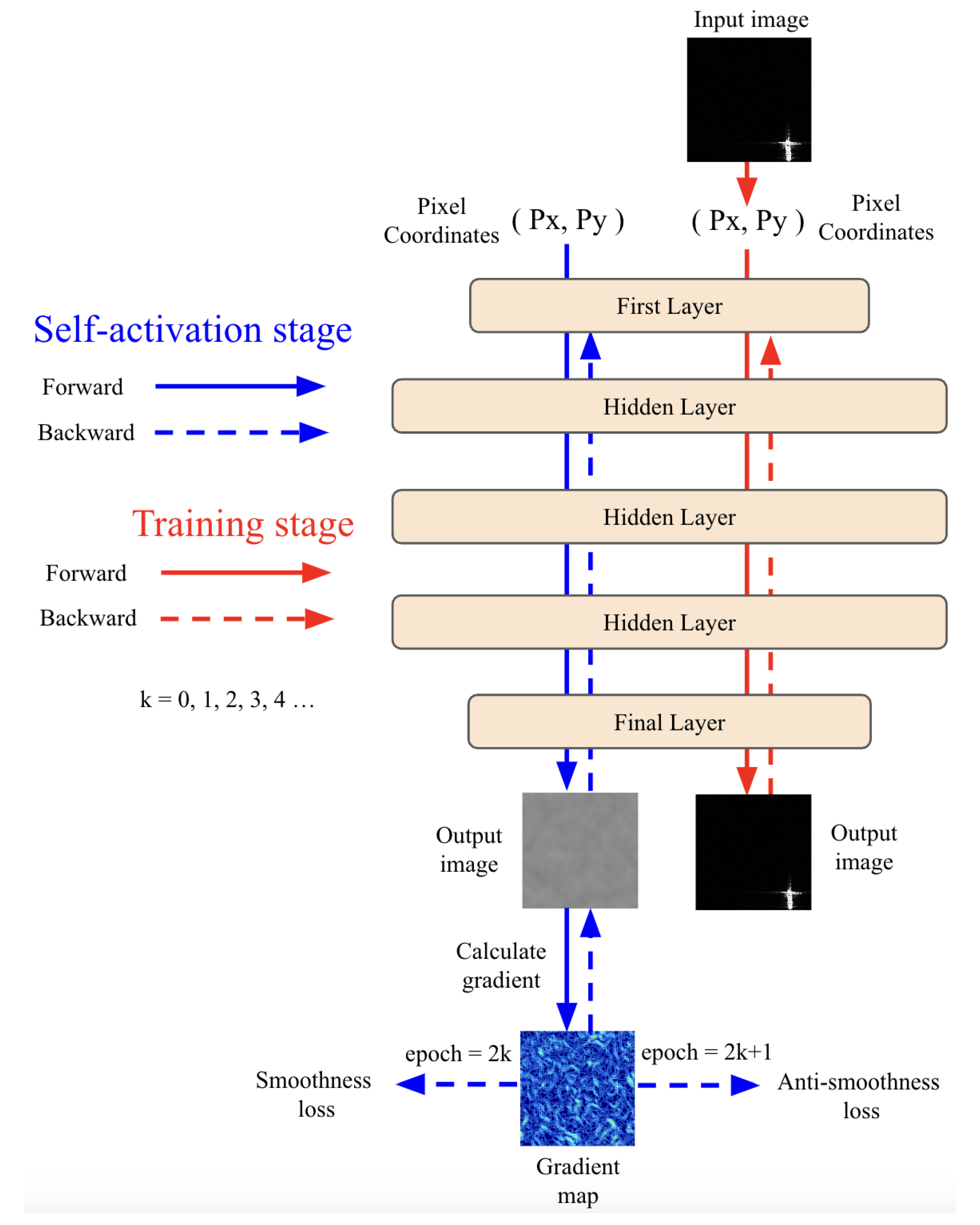
Our proposed method with the self-activation stage is illustrated in Figure 2. Instead of directly learning the Implicit Neural Representations (INRs) for the target SAR image, we first initialize the INR model using a self-activation method that does not rely on any information from the target image during training. In the self-activation stage, we alternately apply two opposing functions to the model’s output. Upon completing the self-activation stage, we use the activated model to learn the representation of the SAR image.

Self-Activated INR

In INR models for signal learning tasks, previous works highlight the importance of proper model weight initialization for effectively fitting and capturing the fine details of images. Inspired by the effectiveness of network initialization in improving INR model performance, we explore the possibility of activating the model weights before target training. Since the model is activated prior to learning the target signal, it is not possible to make a model learn any information from the target image during this stage. Consequently, we propose a self-activation method that utilizes the loss function on the model output to activate the model weights by leveraging the cross-pixel relationships within the output.

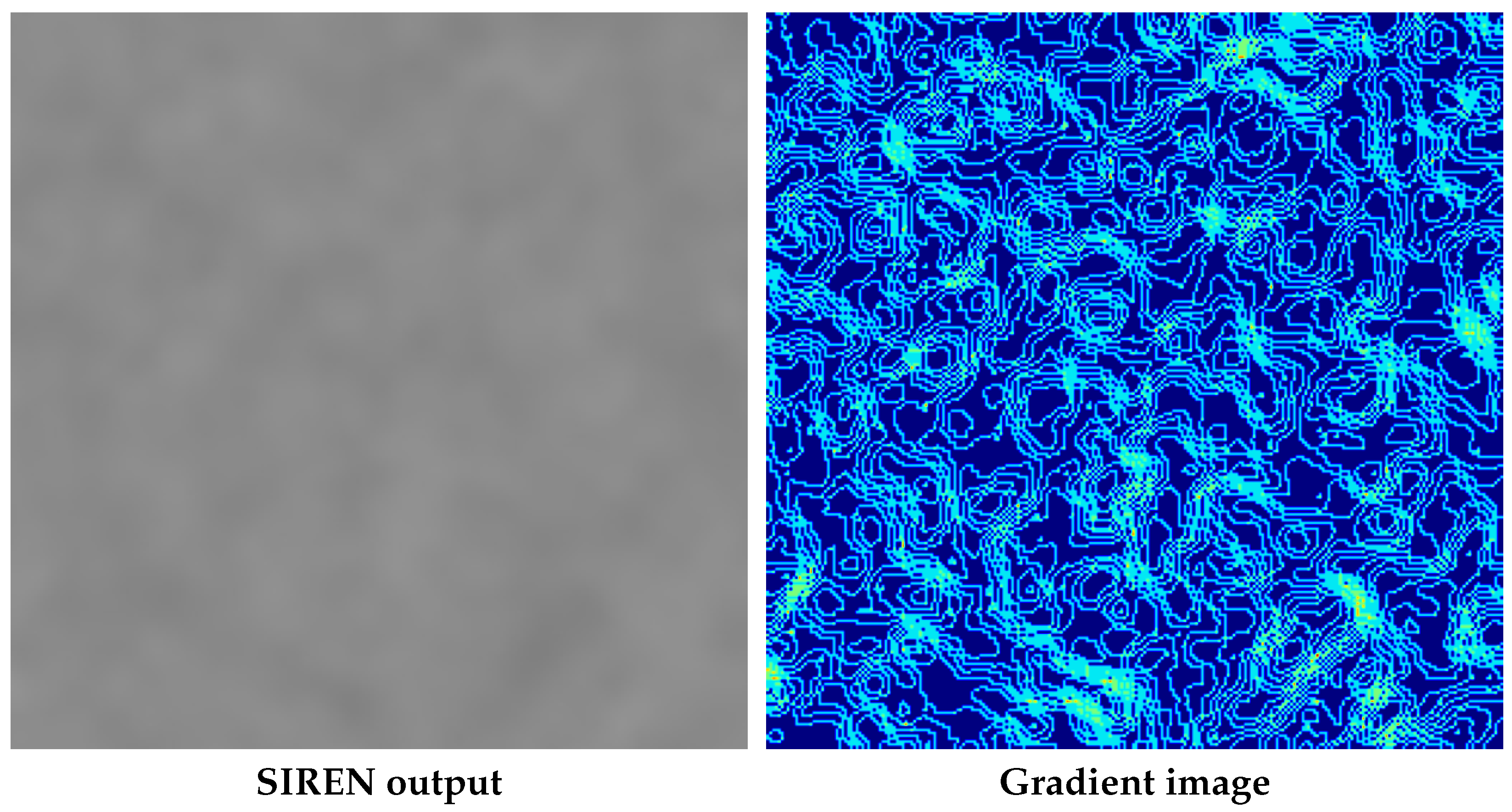
In the self-activation method, the two opposing loss functions are calculated based on the gradient maps of the model’s output image. The gradient map of an image reflects the variation in pixel values and serves as an effective representation of cross-pixel relationships. In the gradient map, $G\left(I\right)$, pixels in coarse regions with significant differences from neighboring pixels exhibit larger gradient values, while pixels in smooth areas, where values are similar to neighboring pixels, show smaller gradient values. We employ the Sobel operator to approximate the image gradient, which is a convolution-based discrete method utilizing two Sobel kernels, $K_x$ and $K_y$, formulated as follows:

$$G\left(I\right)=\sqrt{{(I\ast K_x)}^2+{(I\ast K_y)}^2}.$$

(7)

Using the Sobel operator, we calculate the gradient maps of the model’s output image, which does not incorporate any knowledge from the target but instead relies on the model’s vanilla initialization. As shown in Figure 3, we observe that the model’s output is not a flattened image but rather a nearly gray image with complex textures, presenting distinct cross-pixel relationships.

Based on the gradient maps of the model’s output image, we alternately apply two opposing loss functions during the self-activation stage: a smoothness loss to increase the image gradient and an anti-smoothness loss to reduce it, thereby exploiting cross-pixel relationships to activate the INR model. The anti-smoothness and smoothness loss function alternate across different training epochs, e: the anti-smoothness loss function is applied during even-numbered epochs, while the smoothness loss function is applied during odd-numbered epochs. To calculate the smoothness loss, we acquire the gradient map of the model’s original output, compute the average gradient across the entire image, and take this value as the loss, which can be formulated as follows:

$${\mathcal{L}}_{smoothness}={\displaystyle \frac{1}{W·H}}\sum _{i=1}^W\sum _{j=1}^{H}G\left(I\right),$$

(8)

Consequently, the smoothness loss function reduces the difference in pixel values with their neighbors in the output image, which restores cross-pixel relationships. The anti-smoothness loss function also computes the average gradient across the entire image, but unlike the first loss function we take the negative of this value and use it as the loss, which can be formulated as follows:

$${\mathcal{L}}_{anti-smoothness}=-\left({\displaystyle \frac{1}{W·H}}\sum _{i=1}^W\sum _{j=1}^{H}G\left(I\right)\right).$$

(9)

The anti-smoothness loss function increases the difference between a pixel’s value and its neighbors in the output image, thereby disturbing the relationships between pixels. Therefore, our final opposite loss function, which alternately applies smoothness and anti-smoothness loss, can be formulated as follows:

$${\mathcal{L}}_{oppsite}=a·\gamma ·{\mathcal{L}}_{smoothness}+(1-a)·\gamma ·{\mathcal{L}}_{anti-smoothness},a=\left\{\begin{array}{cc}0\hfill & \mathrm{if}e\mathrm{is}\mathrm{even}\hfill \\ 1\hfill & \mathrm{if}e\mathrm{is}\mathrm{odd}\hfill \end{array}\right.$$

(10)

where $\gamma$ is a scaling coefficient with a default value set to 0.2. Based on our INR model in the self-activation stage, we learn the network parameters, $\theta$, of the target image function, $f_{\theta }(P_x,P_y)$, which can be formulated as follows:

$$\begin{array}{c}\hfill {\theta }^{\ast }=\left\{\begin{array}{cc}arg\underset{\theta }{min}{\mathcal{L}}_{oppsite}(P_x,P_y),\hfill & e<p\hfill \\ arg\underset{\theta }{min}{\mathcal{L}}_{MSE}\left(f_{\theta }(P_x,P_y)\right),\hfill & e\ge p\hfill \end{array}\right..\end{array}$$

(11)

Here, p represents the number of epochs of the self-activation stage, which utilizes the training frequency of ${\mathcal{L}}_{opposite}$. We self-activate the INR model using the opposite loss function for p epochs and then utilize this self-activated model to learn the continuous representation of SAR images.

3.2. Analysis by Neural Tangent Kernel

Our work applies such pre-activation to Image INR and introduces a novel self-activation method by mitigating access to the target image during the pre-training stage. After pre-training, the model weights enter into a mode that is more appropriate for capturing high-frequency details, which are essential for guaranteeing high performance in image INRs. To illustrate this, we use the Neural Tangent Kernel (NTK) [48] to analyze the network’s weights. Specifically, the network’s capability to learn signals is closely tied to the NTK’s diagonal characteristics, where strong diagonal dominance promotes shift invariance and accelerates the capture of fine-detail components. Let $f(x;\theta )$ denote the computational graph of a given neural network, where x represents the input and $\theta$ represents the network parameters. The neural tangent kernel is defined as

$$\mathcal{K}(x_i,x_j)={\nabla }_{\theta }f(x_i;{\theta }_0){\nabla }_{\theta }f{(x_j;{\theta }_0)}^{\top },$$

(12)

where $\mathcal{K}(x_i,x_j)$ is the element in the i-th row and j-th column of the empirical NTK matrix, corresponding to the i-th sample $x_i$ and the j-th sample $x_j$. According to references [49], NTKs with stronger diagonal characteristics exhibit better translation invariance. This implies that the coordinates in the training set are nearly decoupled from one another during the training process, facilitating more effective signal learning.

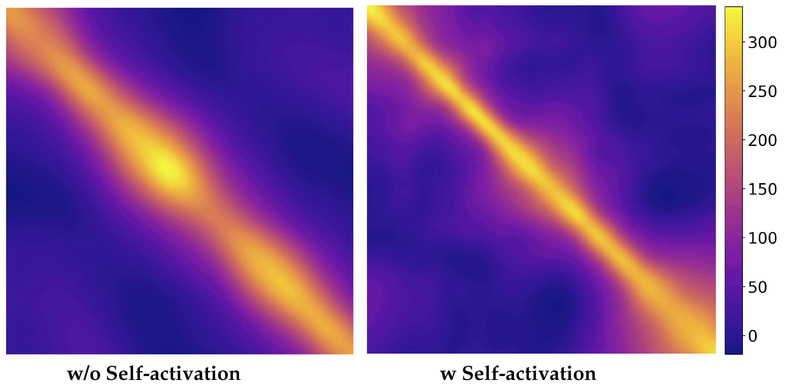
We define a signal with a one-dimensional coordinate of size 1024 as our learning target and visualize the corresponding NTKs both with and without the self-activation stage of the INR model, as illustrated in Figure 4. Our analysis reveals that the diagonal property of the NTK is significantly enhanced with the self-activated INR model. This indicates that incorporating the self-activation stage in the INR model provides better shift invariance compared to directly learning the target signal, along with an enhanced ability to capture high-frequency components.

4. Experiments

4.1. Implementation Details and Evaluation Metrics

We carried out all experiments using PyTorch version 1.11.0, applying the Adam optimizer. The optimization was performed on a system with 64 GB of RAM, utilizing an NVIDIA RTX A2000 graphics processing unit for computational tasks. Apart from our self-activation stage, when learning the target image we use the MSE loss function to train the model by comparing the measurements with the outputs of the INR, and we follow the training setup that we used for the baseline INR models.

We evaluate the INR model’s reconstruction image quality and reconstruction performance using two commonly used metrics: Peak-Signal-to-Noise-Ratio (PSNR) and Structural Similarity Index Measure (SSIM) [50]. PSNR measures the ratio between the original image and the difference between the original and the reconstructed image. It is calculated using the formula

$$PSNR(x,y)=10·{log}_{10}\left({\displaystyle \frac{MA{X}_I^2}{MSE}}\right),$$

(13)

where $MA{X}_I$ is the original image’s pixel value and $MSE$ is the mean squared error between the original and reconstructed image. Higher PSNR values indicate better image quality. On the other hand, SSIM evaluates the similarity between two images by taking into account structural information, luminance, and contrast. SSIM values range from −1 to 1, with a value of 1 indicating perfect similarity. It is calculated using the formula

$$SSIM(x,y)={\displaystyle \frac{(2{\mu }_x{\mu }_y+C_1)(2{\sigma }_{xy}+C_2)}{({\mu }_x^2+{\mu }_y^2+C_1)({\sigma }_x^2+{\sigma }_y^2+C_2)}},$$

(14)

where ${\mu }_x$ and ${\mu }_y$ are the mean values of the images x and y, ${\sigma }_x^2$ and ${\sigma }_y^2$ are their variances, ${\sigma }_{xy}$ is the covariance, and $C_1$ and $C_2$ are small constants that stabilize the division. Together, PSNR and SSIM provide complementary insights into the fidelity and perceptual quality of reconstructed images.

4.2. Datasets

SARDet-100K is a newly created large-scale [51], multi-category benchmark dataset for SAR object detection, combining 10 existing public SAR datasets. It contains approximately 117,000 images and 246,000 object instances, covering six major categories: aircraft, ships, cars, bridges, tanks, and harbors. These images are sourced from various SAR satellite platforms, such as Sentinel-1 [52], TerraSAR-X [53], and Gaofen-3 [54]. SARDet-100K is the first SAR object detection dataset to reach COCO scale, featuring not only diverse target types but also a wide range of scene variations, including different imaging angles, weather conditions, and land cover types. These characteristics make it a broader and more complex experimental foundation for SAR object detection research compared to MSTAR [55] and SSDD [56]. Additionally, SARDet-100K standardizes the resolution and annotation formats of all datasets, ensuring consistency in model training and testing while providing researchers with an efficient platform for evaluating different detection methods. Notably, both the scale and diversity of SARDet-100K enhance the robustness of detection models in complex scenarios and help researchers better understand common noise and artifacts in SAR imagery. Furthermore, when paired with the newly proposed MSFA pre-training framework, which incorporates multi-stage pre-training and filter-augmented input, SARDet-100K significantly reduces the domain gap between RGB and SAR images in the feature space, thereby improving object detection performance.

4.3. SAR Image Reconstruction

In SAR image reconstruction experiments, we attempt to parameterize a function that maps pixel coordinates, $\varphi :{\mathbb{R}}^2\to {\mathbb{R}}^1$, to pixel values, $x\mapsto f\left(x\right)$, representing a discrete image in a continuous fashion using a model. We randomly select 20 SAR images from the SARDet-100K dataset as a learning target for image reconstruction. Given a target SAR image, we select four state-of-the-art INR models as baseline models for learning and compare their performance with and without the self-activation method, including Sinusoidal Representation Network (SIREN) [20], Gaussian activation function-based INRs (Gauss) [47], Flexible Spectral-Bias Tuning in Implicit Neural Representations (FINER) [57], and Wavelet Implicit Neural Representations (WIRE) [21]. Among them, SIREN, a seminal INR model, demonstrates that periodic functions can accurately fit signals with a sophisticated initialization method. Moreover, both WIRE and FINER propose initialization methods for their INR models that are suitable for continuous complex Gabor wavelets and flexible spectral-bias tuning. We adopt their default initialization method, configuring these INR models with three hidden layers, each containing 256 neurons, to ensure fairness. By default, using the self-activated method, we first set a self-activation stage for 200 epochs, during which the model is trained with our opposing loss. Following this, the self-activated model is used to learn the target image, and the results are compared to the ground truth. Without the self-activated method, the aforementioned INR models are directly used to learn the image signal.

The quantitative results of the PSNR and SSIM evaluation metrics for various INR models trained with and without self-activation are presented side by side in

Table 1. Experimental evaluation of SAR image reconstruction performance, contrasting results from models with and without self-activation.

Metrics	SIREN		Gauss		WIRE		FINER
	w/o SA	w SA	w/o SA	w SA	w/o SA	w SA	w/o SA	w SA
PSNR	31.05	35.27	32.15	36.35	30.42	35.36	37.17	42.01
SSIM	0.8567	0.8989	0.8821	0.9372	0.8208	0.9313	0.9427	0.9693

for comparative analysis. We observe that for all INR models that we selected, conducting self-activation before learning the target image can significantly improve model reconstruction performance. Specifically, using SIREN as the baseline model, our self-activation method improves PSNR by 4.22 and SSIM by 0.0422, achieving values of 35.27 and 0.8989, respectively. Moreover, the WIRE model demonstrates the most significant improvement compared to its performance without self-activation, showing increases of 4.94 in PSNR and 0.1105 in SSIM. In FINER, direct learning signals can also yield competitive results, achieving a PSNR of 37.17 and an SSIM of 0.9427, while the application of the self-activation method further enhances these values to 42.01 and 0.9693, respectively. Our proactive method is compatible with the initialization methods specific to each INR model. We also visualize the reconstruction results to compare the qualitative outcomes of various INR models with and without the self-activation method, as shown in Figure 5. Through our detailed comparison, we demonstrate that our method can effectively reconstruct noise information and high-frequency areas in the SAR images, making the reconstruction results closer to the ground truth. This indicates that the INR model’s capability to capture high-frequency components in images is enhanced after self-activation.

In the SARDet-100K dataset, which contains six categories—ship, aircraft, bridge, tank, car, and harbor—categories such as ship, car, and tank typically appear in simpler environments, making their images easier to reconstruct. However, categories like bridges and harbors are often captured in urban environments, resulting in images that contain a wealth of radar reflection information and incorporate numerous objects and textures, which lead to more intricate images that are challenging to reconstruct and ultimately lower reconstruction accuracy. We randomly selected 20 images from each category as the reconstruction targets, comparing the performance of various INR models trained with and without self-activation. As shown in

Table 2. Quantitative assessment of image reconstruction performance across various classes of SARDet-100K, comparing models with and without self-activation.

Model	SA	PSNR/SSIM
		Aircraft	Ship	Car	Bridge	Tank	Harbor
SIREN	w/o SA	31.32/0.8612	32.05/0.8671	32.15/0.8695	29.12/0.7848	31.40/0.8825	28.50/0.7855
	w SA	35.27/0.9104	36.12/0.9184	36.63/0.9118	34.95/0.8537	37.25/0.9461	34.15/0.8670
Gauss	w/o SA	32.44/0.9340	34.15/0.9286	33.82/0.9774	30.01/0.8165	35.60/0.9734	29.72/0.8040
	w SA	36.18/0.9431	37.50/0.9398	37.92/0.9875	35.78/0.8778	39.42/0.9799	35.05/0.8801
WIRE	w/o SA	31.10/0.8278	31.02/0.8335	31.06/0.8370	28.65/0.7791	31.22/0.8412	28.10/0.7722
	w SA	35.30/0.9318	35.48/0.9364	35.82/0.9410	34.20/0.8492	36.07/0.9340	34.02/0.8510
FINER	w/o SA	37.62/0.9460	38.25/0.9481	38.45/0.9490	35.82/0.9116	42.60/0.9664	37.20/0.9105
	w SA	41.89/0.9682	42.15/0.9710	43.32/0.9745	40.72/0.9543	45.12/0.9792	40.60/0.9420

, our self-activation method improves model performance across all categories, including the challenging bridge and harbor categories, further demonstrating that our method is applicable to a wide range of images.

4.4. High-Resolution SAR Image Reconstruction

With the continuous representation of images, image resolution is closely linked to the difficulty of learning image representations using the INR model. High resolution implies that images contain more information, leading to more complex functions compared to low-resolution images, which poses a challenge for the INR model to learn effectively. Therefore, we conduct experiments to investigate whether or not our self-activation method enhances the learning of challenging high-resolution images across various INR models. The CARABAS-II [58] is a high-resolution airborne VHF Synthetic Aperture Radar (SAR) dataset, collected from a wide area at a depression angle for low-frequency radar imaging, operating in the frequency range of 20–90 MHz. Its main feature is the ability to penetrate dense vegetation, forests, and other complex terrain structures. Through advanced imaging algorithms and signal processing techniques, CARABAS-II enhances the imaging quality of targets while maintaining strong penetration capabilities, providing clear images of targets hidden underground or behind obstacles. The CARABAS-II dataset covers various complex scenarios, including forests, deserts, and urban environments. Its low-frequency imaging capability significantly improves the detection of concealed targets. Compared to high-frequency SAR data, CARABAS-II is more suitable for target detection in challenging terrains, allowing researchers to better understand target scattering characteristics and signal reflection patterns in low-frequency environments. Based on the high-resolution SAR image dataset of CARABAS-II, which is widely used in various fields, we explore the performance of our self-activation method in reconstructing these high-resolution images.

We randomly select five high-resolution images from the CARABAS-II dataset for image reconstruction to evaluate the effectiveness of our self-activation method. We use SIREN [20], Gauss [47], WIRE [47], and FINER [17] as baseline models and compare the results with and without the self-activation method. To prevent the high computational demands of learning high-resolution images from causing memory issues, we perform two iterations at each epoch and carry out gradient backpropagation. Based on the challenges posed by high-resolution SAR images, we set the self-activation epoch to 300 and learn the target image for 500 epochs, comparing the results with those obtained by directly using the INR model to learn the target image without self-activation. As shown in

Table 3. Experimental evaluation of high-resolution SAR image reconstruction performance, contrasting results from models with and without self-activated.

Metrics	SIREN		Gauss		WIRE		FINER
	w/o SA	w SA	w/o SA	w SA	w/o SA	w SA	w/o SA	w SA
PSNR	20.33	20.82	21.89	22.50	21.14	21.57	21.68	22.24
SSIM	0.2107	0.2473	0.3827	0.4103	0.3539	0.3736	0.3336	0.3961

, we find that the self-activated INR model achieves a non-trivial improvement in challenging high-resolution images, including an enhancement of 0.61 in PSNR and 0.0286 SSIM for SIREN. This indicates that our method can also be effective for high-resolution images, improving reconstruction accuracy. We visualize the reconstruction details of various INR models, comparing outputs from models with and without self-activation, as shown in Figure 6. For instance, in the region where object TGB11 is located in the SAR image, the model with self-activation reconstructs finer details compared to direct image learning.

4.5. Ablation Study

To assess the contribution of each component in our self-activation method, we conduct an ablation study using the SARDet-100K dataset. For this, we select 20 images, resize them to 256 × 256, and normalize pixel coordinates to the range (−1,1), consistent with the preprocessing steps in baseline SIREN studies, and adopt the same learning rate and optimizer settings.

4.5.1. Ablation Study of the Opposite Loss Function

The opposite loss function used in our self-activation method consists of smoothness and anti-smoothness losses. The smoothness loss increases the differences between cross-pixels in the output image, while the anti-smoothness loss reduces them. We conduct an ablation study to explore the role of each loss component in the self-activation stage, examining the effects of separately increasing or reducing neighbor pixel differences in the output image. Specifically, we apply either the smoothness or anti-smoothness loss individually during the self-activation of the INR model for 200 epochs, followed by directly learning the target image signal and comparing the image reconstruction results. The results are presented in

Table 4. Ablation study of different loss functions employed during the self-activation stage.

Metrics	Baseline	Anti-Smoothness	Smoothness	Alternation
PSNR	31.05	29.99	31.75	35.27
SSIM	0.8502	0.7648	0.8418	0.8989

; we find that using only the anti-smoothness loss to self-activated the INR model results in a 2.06 PSNR and 0.0854 SSIM decrease compared to the baseline, which directly learns the target image. Self-activating the INR model with the smoothness loss improves reconstruction accuracy by 0.70 PSNR compared to the baseline; however, it still results in a reduction of 3.52 PSNR and 0.0571 SSIM compared to using the opposite loss. Moreover, we present the PSNR vs. epochs curves for the reconstruction of the target image using different self-activation methods with various loss functions, as shown in Figure 7. These results indicate that only by continuously balancing the two opposite losses to control cross-pixel relationships can the model’s performance be significantly improved. Simply increasing or decreasing the differences between pixels has little effect and may even overwhelm the model’s performance.

4.5.2. Ablation Study of the Scaling Coefficient

The scaling coefficient, $\gamma$, of the loss function influences the extent to which cross-pixel relationships transform during the self-activation stage. We conduct an ablation study with various scaling coefficients set at 0.05, 0.1, 0.2, 0.5, 0.7, 1, and 10, comparing these results with the baseline without the self-activation stage. We self-activated the INR model for 200 epochs, followed by 500 epochs of learning the target image. As shown in

Table 5. Ablation study of the scaling coefficient $\gamma$.

Metrics	Baseline	0.05	0.1	0.2	0.5	1	10
PSNR	31.05	34.98	35.17	35.27	35.10	34.83	32.10
SSIM	0.8502	0.8910	0.8971	0.8989	0.8857	0.8801	0.8303

, setting $\gamma$ to 0.2 yielded superior model performance, with PSNR and SSIM values of 35.27 and 0.8989, respectively. However, continuing to increase the scaling coefficient leads to a decline in accuracy, reaching 32.10 PSNR. The results indicate that, during the self-activation stage, appropriately disturbing cross-pixel relationships can significantly improve the model’s performance, and we set the scaling coefficient to 0.2 as our default setting.

4.5.3. Ablation Study on Self-Activation Epochs

The number of epochs in the self-activation stage directly impacts the extent of model activation in the INR model. Too few epochs render the self-activation ineffective, while too many waste valuable computational resources. We perform an ablation study on the self-activation stage to explore whether or not an indefinite increase in self-activation stage epochs benefits the INR model’s learning of target signals. Specifically, we self-activated the INR model with 0, 50, 100, 200, 300, and 400 epochs, learning the target signals at each stage and comparing their image reconstruction accuracy. As shown in

Table 6. Ablation study on self-activation epochs.

Metrics	Baseline	50	100	200	300	400
PSNR	31.05	33.01	34.00	35.27	36.19	35.11
SSIM	0.8602	0.8717	0.8905	0.8989	0.9096	0.8972

, model performance improves as the number of self-activation epochs increases up to 300, with stabilization occurring between 200 and 300 epochs. Beyond this point, further increasing the number of self-activation epochs results in no significant improvement in image accuracy and even shows a slight decline. Moreover, we present the PSNR vs. epochs curves for the reconstruction of the target image across different epoch stages using self-activation, as shown in Figure 8. We observe that the performance improvements obtained through our self-activation method persist throughout the entire process of training the model on the target signal. The largest improvement occurs when the number of epochs in the self-preactivation stage is set to 200. Given the computational and time costs of training, we set the default number of self-activation epochs to 200.

4.5.4. Ablation Study on the Regulation of Various Cross-Pixel Relationships

In our self-activation stage, the anti-smoothness and smoothness, two opposing losses, compute the output image gradients to regulate the cross-pixel relationships in the model’s output. However, beyond image gradients, there are various methods to control cross-pixel relationships in images. We conduct an ablation study to explore utilizing various methods to regulate the cross-pixel relationships. Specifically, apart from calculating the gradient maps with the Sobel kernel, we also select the Laplacian kernel, which can be formulated as follows:

$$K_{\mathrm{Sobel}}=\left[\begin{array}{ccc}-1& 0& 1\\ -2& 0& 2\\ -1& 0& 1\end{array}\right],K_{\mathrm{Laplacian}}=\left[\begin{array}{ccc}-1& -1& -1\\ -1& 8& -1\\ -1& -1& -1\end{array}\right].$$

(15)

Moreover, we also use the standard deviation of the output image to adjust the cross-pixel relationships in the model’s output. As shown in

Table 7. Ablation study on utilizing various methods to regulate cross-pixel relationships.

Metrics	Std	Laplacian	Sobel
PSNR	26.83	34.53	35.27
SSIM	0.7120	0.8871	0.8989

, we observe that utilizing the Sobel kernel in the anti-smoothness and smoothness losses achieves the best model performance, with a PSNR of 35.27 and an SSIM of 0.8989. Moreover, we find that utilizing the standard deviation in our loss function has no effect and can overwhelm the model’s performance. Therefore, we default to using the Sobel kernel in our two opposing loss functions to exploit cross-pixel relationships.

5. Discussion

The Equivalent Number of Looks (ENL) is a widely used metric in SAR imaging to assess model output quality [59,60,61]. For image representation, a model output’s ENL closer to the ground-truth ENL indicates better representation, especially in areas with fine details. We compare the ENL of the target image on the SIREN model, both with and without the self-activation method, as shown in

Table 8. Quantitative Comparison of ENL.

Metrics	Ground Truth	With Self-Activation	Without Self-Activation
ENL	4.21	4.39	4.93

. With our self-activation stage, the model output achieves an ENL of 4.39, which is closer to the ground-truth value of 4.21, compared to the ENL of 4.88 obtained without the self-activation method.

The Kullback–Leibler (KL) distance is a commonly used metric in SAR imaging to evaluate the similarity between the ground truth and generated outputs [62,63], with lower values indicating closer alignment. As shown in

Table 9. Quantitative Comparison of KL distance.

Metrics	SIREN	w SA SIREN
KL Distance	0.0189	0.0103

, we compare the KL distance of SIREN outputs with and without the self-activation method. With self-activation applied, we observe a decrease in the KL distance of the model’s reconstruction from 0.0189 to 0.0103 compared to the baseline SIREN.

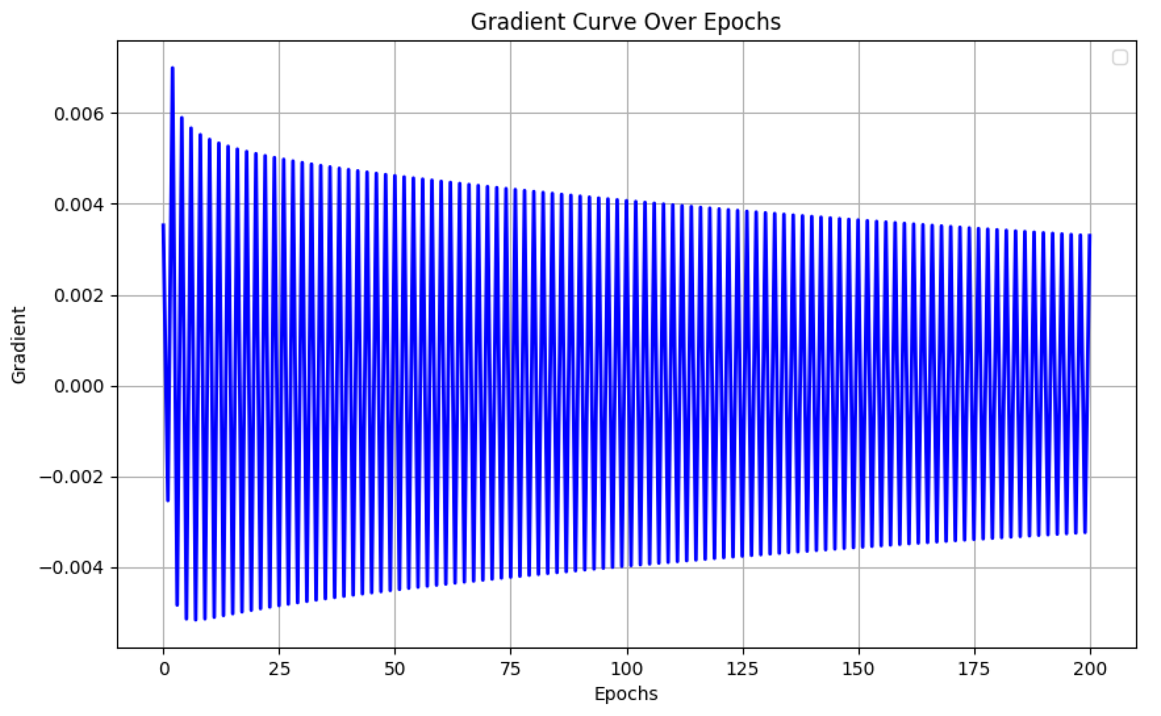
Since our two opposing loss functions alter the gradient of the model’s output image, imbalances may manifest as either exploding gradients or gradients that drop to zero. We prevent this by using opposite loss functions with equal loss weights. We find that this practice is sufficient for guaranteeing stable gradients even after 200 epochs. Empirically, we find that, after 200 epochs, the magnitude of the gradient only has a moderate drop (see Figure 9). This moderate drop can be further mitigated by applying a slightly higher loss weight to the anti-smooth loss component. However, we note that mitigating this moderate drop by sophisticated search on the loss weight yields a very marginal performance boost. Therefore, we stick to using the strategy of equal loss weights for its simplicity and effectiveness.

6. Conclusions

We conducted a pioneering study on using INR for continuous SAR image representation and found that the INR model benefits from previous self-activation before learning the target image. We propose a self-activation method that leverages the model’s initial output of cross-pixel relationships, which does not require any target image-related information as input. The self-activation method utilizes two opposing loss functions (smoothness and anti-smoothness loss) to activate the model, addressing the issue of image information not being input during the activation function stage. We calculate and compare the NTK of the model trained with and without our self-activation method. After applying self-activation, we observe that the NTK exhibits a stronger diagonal structure, indicating an enhanced capacity for learning fine details, including high-frequency components. Overall, our experimental results suggest that our self-activation method can enhance the ability of several state-of-the-art INR models to express signal details, resulting in more competitive outcomes.

References

1. Tewari, A.; Thies, J.; Mildenhall, B.; Srinivasan, P.; Tretschk, E.; Yifan, W.; Lassner, C.; Sitzmann, V.; Martin-Brualla, R.; Lombardi, S.; et al. Advances in neural rendering. Comput. Graph. Forum 2022, 41, 703–735. [Google Scholar] [CrossRef]
2. Sitzmann, V.; Zollhöfer, M.; Wetzstein, G. Scene representation networks: Continuous 3d-structure-aware neural scene representations. In Proceedings of the Advances in Neural Information Processing Systems, Vancouver, BC, Canada, 8–14 December 2019; Volume 32. [Google Scholar]
3. Tancik, M.; Srinivasan, P.; Mildenhall, B.; Fridovich-Keil, S.; Raghavan, N.; Singhal, U.; Ramamoorthi, R.; Barron, J.; Ng, R. Fourier features let networks learn high frequency functions in low dimensional domains. Adv. Neural Inf. Process. Syst. 2020, 33, 7537–7547. [Google Scholar]
4. Fridovich-Keil, S.; Tancik, M.; Mildenhall, B.; Barron, J.; Ramamoorthi, R. Neural Fields for 3D Shape Reconstruction and Representation. In Proceedings of the International Conference on Learning Representations (ICLR), Vienna, Austria, 4 May 2021. [Google Scholar]
5. Verma, S.; Chowdhury, R.; Das, S.K.; Franchetti, M.J.; Liu, G. Sunlight Intensity, Photosynthetically Active Radiation Modelling and Its Application in Algae-Based Wastewater Treatment and Its Cost Estimation. Sustainability 2021, 13, 11937. [Google Scholar] [CrossRef]
6. Reigber, A.; Scheiber, R.; Jager, M. Very-high-resolution airborne synthetic aperture radar imaging: Signal processing and applications. Proc. IEEE 2012, 101, 759–783. [Google Scholar] [CrossRef]
7. Xu, G.; Xing, M.D.; Xia, X.G. High-resolution inverse synthetic aperture radar imaging and scaling with sparse aperture. IEEE J. Sel. Top. Appl. Earth Obs. Remote Sens. 2015, 8, 4010–4027. [Google Scholar] [CrossRef]
8. Bu, X.; Zhang, Z.; Chen, L. Implementation of vortex electromagnetic waves high-resolution synthetic aperture radar imaging. IEEE Antennas Wirel. Propag. Lett. 2018, 17, 764–767. [Google Scholar] [CrossRef]
9. He, Y.; Xu, L.; Huo, J. A Synthetic Aperture Radar Imaging Simulation Method for Sea Surface Scenes Combined with Electromagnetic Scattering Characteristics. Remote Sens. 2024, 16, 3335. [Google Scholar] [CrossRef]
10. Huang, P.; Wu, P.; Guo, Z.; Ye, Z. 3D Light-Direction Sensor Based on Segmented Concentric Nanorings Combined with Deep Learning. Micromachines 2024, 15, 1219. [Google Scholar] [CrossRef]
11. Cheng, K.; Dong, Y. An Image Compensation-Based Range–Doppler Model for SAR High-Precision Positioning. Appl. Sci. 2024, 14, 8829. [Google Scholar] [CrossRef]
12. Ntziachristos, V.; Bremer, C.; Weissleder, R. Fluorescence imaging with near-infrared light: New technological advances that enable in vivo molecular imaging. Eur. Radiol. 2003, 13, 195–208. [Google Scholar] [CrossRef]
13. Zhang, J. Multi-source remote sensing data fusion: Status and trends. Int. J. Image Data Fusion 2010, 1, 5–24. [Google Scholar] [CrossRef]
14. Zheng, S.; Hao, X.; Zhang, C.; Zhou, W.; Duan, L. Towards Lightweight Deep Classification for Low-Resolution Synthetic Aperture Radar (SAR) Images: An Empirical Study. Remote Sens. 2023, 15, 3312. [Google Scholar] [CrossRef]
15. Shin, S.; Kim, Y.; Hwang, I.; Kim, J.; Kim, S. Coupling Denoising to Detection for SAR Imagery. Appl. Sci. 2021, 11, 5569. [Google Scholar] [CrossRef]
16. Liu, S.; Liu, T.; Gao, L.; Li, H.; Hu, Q.; Zhao, J.; Wang, C. Convolutional Neural Network and Guided Filtering for SAR Image Denoising. Remote Sens. 2019, 11, 702. [Google Scholar] [CrossRef]
17. Liu, Z.; Zhu, H.; Zhang, Q.; Fu, J.; Deng, W.; Ma, Z.; Guo, Y.; Cao, X. FINER: Flexible spectral-bias tuning in Implicit NEural Representation by Variable-periodic Activation Functions. In Proceedings of the IEEE/CVF Conference on Computer Vision and Pattern Recognition, Seattle, WA, USA, 16–22 June 2024; pp. 2713–2722. [Google Scholar]
18. Zhang, K.; Zhu, D.; Min, X.; Zhai, G. Implicit neural representation learning for hyperspectral image super-resolution. IEEE Trans. Geosci. Remote Sens. 2022, 61, 1–12. [Google Scholar]
19. Molaei, A.; Aminimehr, A.; Tavakoli, A.; Kazerouni, A.; Azad, B.; Azad, R.; Merhof, D. Implicit neural representation in medical imaging: A comparative survey. In Proceedings of the IEEE/CVF International Conference on Computer Vision, Paris, France, 2–6 October 2023; pp. 2381–2391. [Google Scholar]
20. Sitzmann, V.; Martel, J.; Bergman, A.; Lindell, D.; Wetzstein, G. Implicit neural representations with periodic activation functions. Adv. Neural Inf. Process. Syst. 2020, 33, 7462–7473. [Google Scholar]
21. Saragadam, V.; LeJeune, D.; Tan, J.; Balakrishnan, G.; Veeraraghavan, A.; Baraniuk, R.G. Wire: Wavelet implicit neural representations. In Proceedings of the IEEE/CVF Conference on Computer Vision and Pattern Recognition, Vancouver, BC, Canada, 17–24 June 2023; pp. 18507–18516. [Google Scholar]
22. Saxena, R.; Singh, K. Fractional Fourier transform: A novel tool for signal processing. J. Indian Inst. Sci. 2005, 85, 11. [Google Scholar]
23. Sandryhaila, A.; Moura, J.M. Discrete signal processing on graphs: Graph fourier transform. In Proceedings of the 2013 IEEE International Conference on Acoustics, Speech and Signal Processing, Vancouver, BC, Canada, 26–31 May 2013; pp. 6167–6170. [Google Scholar]
24. Lundén, J.; Koivunen, V. Automatic radar waveform recognition. IEEE J. Sel. Top. Signal Process. 2007, 1, 124–136. [Google Scholar] [CrossRef]
25. Paris, S.; Durand, F. A fast approximation of the bilateral filter using a signal processing approach. In Computer Vision–ECCV 2006: 9th European Conference on Computer Vision, Graz, Austria, May 7–13, 2006, Proceedings, Part IV 9; Springer: Berlin/Heidelberg, Germany, 2006; pp. 568–580. [Google Scholar]
26. Chen, Y.; Liu, S.; Wang, X.; Bao, H.; Liu, Y. Learning continuous image representation with local implicit image function. In Proceedings of the IEEE/CVF Conference on Computer Vision and Pattern Recognition, Nashville, TN, USA, 20–25 June 2021; pp. 8628–8638. [Google Scholar]
27. Tretschk, E.; Tewari, A.; Golyanik, V.; Zollhöfer, M.; Lassner, C.; Theobalt, C. Non-rigid neural radiance fields: Reconstruction and novel view synthesis of a dynamic scene from monocular video. In Proceedings of the IEEE/CVF International Conference on Computer Vision, Montreal, BC, Canada, 11–17 October 2021; pp. 12959–12970. [Google Scholar]
28. Xie, S.; Zhu, H.; Liu, Z.; Zhang, Q.; Zhou, Y.; Cao, X.; Ma, Z. DINER: Disorder-invariant implicit neural representation. In Proceedings of the IEEE/CVF Conference on Computer Vision and Pattern Recognition, Vancouver, BC, Canada, 17–24 June 2023; pp. 6143–6152. [Google Scholar]
29. Chen, Z.; Chen, Y.; Liu, J.; Xu, X.; Goel, V.; Wang, Z.; Shi, H.; Wang, X. Videoinr: Learning video implicit neural representation for continuous space-time super-resolution. In Proceedings of the IEEE/CVF Conference on Computer Vision and Pattern Recognition, New Orleans, LA, USA, 18–24 June 2022; pp. 2047–2057. [Google Scholar]
30. Mildenhall, B.; Srinivasan, P.P.; Tancik, M.; Barron, J.T.; Ramamoorthi, R.; Ng, R. Nerf: Representing scenes as neural radiance fields for view synthesis. Commun. ACM 2021, 65, 99–106. [Google Scholar] [CrossRef]
31. Madsen, S.; Edelstein, W.; DiDomenico, L.D.; LaBrecque, J. A geosynchronous synthetic aperture radar; for tectonic mapping, disaster management and measurements of vegetation and soil moisture. In Proceedings of the IGARSS 2001. Scanning the Present and Resolving the Future. Proceedings. IEEE 2001 International Geoscience and Remote Sensing Symposium (Cat. No. 01CH37217), Sydney, NSW, Australia, 9–13 July 2001; Volume 1, pp. 447–449. [Google Scholar]
32. Koo, V.; Chan, Y.K.; Vetharatnam, G.; Chua, M.Y.; Lim, C.H.; Lim, C.S.; Thum, C.; Lim, T.S.; bin Ahmad, Z.; Mahmood, K.A.; et al. A new unmanned aerial vehicle synthetic aperture radar for environmental monitoring. Prog. Electromagn. Res. 2012, 122, 245–268. [Google Scholar] [CrossRef]
33. Ozden, A.; Faghri, A.; Li, M.; Tabrizi, K. Evaluation of Synthetic Aperture Radar satellite remote sensing for pavement and infrastructure monitoring. Procedia Eng. 2016, 145, 752–759. [Google Scholar] [CrossRef]
34. Fernández, M.G.; López, Y.Á.; Arboleya, A.A.; Valdés, B.G.; Vaqueiro, Y.R.; Andrés, F.L.H.; García, A.P. Synthetic aperture radar imaging system for landmine detection using a ground penetrating radar on board a unmanned aerial vehicle. IEEE Access 2018, 6, 45100–45112. [Google Scholar] [CrossRef]
35. Yang, Y.; Qiu, Y.; Lu, C. Automatic target classification-experiments on the MSTAR SAR images. In Proceedings of the Sixth International Conference on Software Engineering, Artificial Intelligence, Networking and Parallel/Distributed Computing and First ACIS International Workshop on Self-Assembling Wireless Network, Towson, MD, USA, 23–25 May 2005; pp. 2–7. [Google Scholar]
36. Breit, H.; Fritz, T.; Balss, U.; Lachaise, M.; Niedermeier, A.; Vonavka, M. TerraSAR-X SAR processing and products. IEEE Trans. Geosci. Remote Sens. 2009, 48, 727–740. [Google Scholar] [CrossRef]
37. Li, Y.; Peng, C.; Chen, Y.; Jiao, L.; Zhou, L.; Shang, R. A deep learning method for change detection in synthetic aperture radar images. IEEE Trans. Geosci. Remote Sens. 2019, 57, 5751–5763. [Google Scholar] [CrossRef]
38. Kang, M.; Ji, K.; Leng, X.; Xing, X.; Zou, H. Synthetic aperture radar target recognition with feature fusion based on a stacked autoencoder. Sensors 2017, 17, 192. [Google Scholar] [CrossRef] [PubMed]
39. Guo, J.; Lei, B.; Ding, C.; Zhang, Y. Synthetic aperture radar image synthesis by using generative adversarial nets. IEEE Geosci. Remote Sens. Lett. 2017, 14, 1111–1115. [Google Scholar] [CrossRef]
40. Chen, C.; He, C.; Hu, C.; Pei, H.; Jiao, L. A deep neural network based on an attention mechanism for SAR ship detection in multiscale and complex scenarios. IEEE Access 2019, 7, 104848–104863. [Google Scholar] [CrossRef]
41. Zhao, P.; Liu, K.; Zou, H.; Zhen, X. Multi-stream convolutional neural network for SAR automatic target recognition. Remote Sens. 2018, 10, 1473. [Google Scholar] [CrossRef]
42. Zhang, F.; Hu, C.; Yin, Q.; Li, W.; Li, H.C.; Hong, W. Multi-aspect-aware bidirectional LSTM networks for synthetic aperture radar target recognition. IEEE Access 2017, 5, 26880–26891. [Google Scholar] [CrossRef]
43. Kim, J.; Lee, Y.; Hong, S.; Ok, J. Learning continuous representation of audio for arbitrary scale super resolution. In Proceedings of the ICASSP 2022—2022 IEEE International Conference on Acoustics, Speech and Signal Processing (ICASSP), Virtual, 7–13 May 2022; pp. 3703–3707. [Google Scholar]
44. Avidan, S.; Shashua, A. Novel view synthesis in tensor space. In Proceedings of the Proceedings of IEEE Computer Society Conference on Computer Vision and Pattern Recognition, San Juan, PR, USA, 17–19 June 1997; pp. 1034–1040. [Google Scholar]
45. Ma, Z.; Liu, S. A review of 3D reconstruction techniques in civil engineering and their applications. Adv. Eng. Inform. 2018, 37, 163–174. [Google Scholar] [CrossRef]
46. Popescu, M.C.; Balas, V.E.; Perescu-Popescu, L.; Mastorakis, N. Multilayer perceptron and neural networks. WSEAS Trans. Circuits Syst. 2009, 8, 579–588. [Google Scholar]
47. Ramasinghe, S.; Lucey, S. Beyond periodicity: Towards a unifying framework for activations in coordinate-mlps. In European Conference on Computer Vision; Springer: Cham, Switzerland, 2022; pp. 142–158. [Google Scholar]
48. Jacot, A.; Gabriel, F.; Hongler, C. Neural tangent kernel: Convergence and generalization in neural networks. In Proceedings of the Advances in Neural Information Processing Systems, Montréal, QC, Canada, 3–8 December 2018; Volume 31. [Google Scholar]
49. Bai, J.; Liu, G.R.; Gupta, A.; Alzubaidi, L.; Feng, X.Q.; Gu, Y. Physics-informed radial basis network (PIRBN): A local approximating neural network for solving nonlinear partial differential equations. Comput. Methods Appl. Mech. Eng. 2023, 415, 116290. [Google Scholar] [CrossRef]
50. Hore, A.; Ziou, D. Image Quality Metrics: PSNR vs. SSIM. In Proceedings of the 2010 20th International Conference on Pattern Recognition, Istanbul, Turkey, 23–26 August 2010; pp. 2366–2369. [Google Scholar] [CrossRef]
51. Li, Y.; Li, X.; Li, W.; Hou, Q.; Liu, L.; Cheng, M.M.; Yang, J. Sardet-100k: Towards Open-Source Benchmark and Toolkit for Large-Scale SAR Object Detection. arXiv 2024, arXiv:2403.06534. [Google Scholar]
52. Torres, R.; Snoeij, P.; Geudtner, D.; Bibby, D.; Davidson, M.; Attema, E.; Potin, P.; Rommen, B.; Floury, N.; Brown, M.; et al. GMES Sentinel-1 mission. Remote Sens. Environ. 2012, 120, 9–24. [Google Scholar] [CrossRef]
53. Lumsdon, P.; Koppe, W.; Hartley, C.; Janoth, J.; Kahabka, H.; Cerezo, F.; Fernandez, V.D.E.; Pérez, J.I.C. Verification of Operational Applications of New Modes of Terrasar-X PAZ Constellation. In Proceedings of the 2021 IEEE International Geoscience and Remote Sensing Symposium IGARSS, Brussels, Belgium, 11–16 July 2021; pp. 7846–7849. [Google Scholar]
54. Shao, W.; Sheng, Y.; Sun, J. Preliminary assessment of wind and wave retrieval from Chinese Gaofen-3 SAR imagery. Sensors 2017, 17, 1705. [Google Scholar] [CrossRef] [PubMed]
55. Ross, T.D.; Bradley, J.J.; Hudson, L.J.; O’connor, M.P. SAR ATR: So what’s the problem? An MSTAR perspective. In Algorithms for Synthetic Aperture Radar Imagery VI; SPIE: Cardiff, UK, 1999; Volume 3721, pp. 662–672. [Google Scholar]
56. Zhang, T.; Zhang, X.; Li, J.; Xu, X.; Wang, B.; Zhan, X.; Xu, Y.; Ke, X.; Zeng, T.; Su, H.; et al. SAR ship detection dataset (SSDD): Official release and comprehensive data analysis. Remote Sens. 2021, 13, 3690. [Google Scholar] [CrossRef]
57. Kawata, S.; Sun, H.B.; Tanaka, T.; Takada, K. Finer features for functional microdevices. Nature 2001, 412, 697–698. [Google Scholar] [CrossRef] [PubMed]
58. Lundberg, M.; Ulander, L.M.; Pierson, W.E.; Gustavsson, A. A challenge problem for detection of targets in foliage. In Algorithms for Synthetic Aperture Radar Imagery XIII; SPIE: Cardiff, UK, 2006; Volume 6237, pp. 160–171. [Google Scholar]
59. Gómez, L.; Cardona-Mesa, A.A.; Vásquez-Salazar, R.D.; Travieso-González, C.M. Analysis of Despeckling Filters Using Ratio Images and Divergence Measurement. Remote Sens. 2024, 16, 2893. [Google Scholar] [CrossRef]
60. Torres, L.; Sant’Anna, S.J.; da Costa Freitas, C.; Frery, A.C. Speckle reduction in polarimetric SAR imagery with stochastic distances and nonlocal means. Pattern Recognit. 2014, 47, 141–157. [Google Scholar] [CrossRef]
61. Cheng, K.; Lam, E.; Standish, B.; Yang, V. Speckle reduction of endovascular optical coherence tomography using a generalized divergence measure. Opt. Lett. 2012, 37, 2871–2873. [Google Scholar] [CrossRef]
62. Qin, X.; Zhang, Y.; Li, Y.; Cheng, Y.; Yu, W.; Wang, P.; Zou, H. Distance measures of polarimetric SAR image data: A survey. Remote Sens. 2022, 14, 5873. [Google Scholar] [CrossRef]
63. Hu, L.; Wang, C. An Evaluation Method of SAR Images Based on Kullback-Leiber Divergence. In Proceedings of the 2015 IEEE 12th Intl Conf on Ubiquitous Intelligence and Computing and 2015 IEEE 12th Intl Conf on Autonomic and Trusted Computing and 2015 IEEE 15th Intl Conf on Scalable Computing and Communications and Its Associated Workshops (UIC-ATC-ScalCom), Beijing, China, 10–14 August 2015; pp. 1611–1616. [Google Scholar]
Figure 1. Overview of the learning INR for the image signal. MLP receives pixel coordinates as input and outputs corresponding pixel values, with weight training guided by MSE loss function.
Remotesensing 16 04473 g001
Figure 2. Pipeline of the proposed method, comprising two stages: the self-activation stage and the training stage. The self-activation stage is performed before the training stage without using any information related to the target. Instead, it leverages smoothness and anti-smoothness losses to exploit the cross-pixel relationships within the model’s own output, thereby pre-activating the model.
Remotesensing 16 04473 g002
Figure 3. Visualization of the INR model SIREN’s initial output (left) and their corresponding gradient maps (right). We observe that the initial output image of SIREN, which has not been trained, is not flattened but possesses a very complex texture.
Remotesensing 16 04473 g003
Figure 4. Visualization of the NTK for the INR model SIREN with and without self-activation. After our self-activation stage, the enhanced diagonal characteristics of the model’s NTK indicate that the model is better at capturing high-frequency components.
Remotesensing 16 04473 g004
Figure 5. Qualitative evaluation of SAR image reconstruction. The first column displays the ground-truth image. Our self-activation method demonstrates enhanced capability in capturing high-frequency details.
Remotesensing 16 04473 g005
Figure 6. Qualitative evaluation of high-resolution SAR image reconstruction. The first column displays the ground-truth image, and we use a red box to highlight and zoom in on the image reconstruction details for better observation. Our self-activation method demonstrates enhanced capability in capturing high-frequency details.
Remotesensing 16 04473 g006
Figure 7. Exhibition of model performance trained with different loss functions during the training stage. Each subfigure illustrates the evolution of PSNR and SSIM metrics throughout the training stage.
Remotesensing 16 04473 g007
Figure 8. Exhibition of model performance with different numbers of self-activation stage epochs. Each subfigure illustrates the evolution of PSNR and SSIM metrics throughout the training stage.
Remotesensing 16 04473 g008
Figure 9. The model output image gradient curve over epochs during our self-activation stage. The directions denote whether the loss component is anti-smoothness or smoothness.
Remotesensing 16 04473 g009