Abstract
The China Seismo-Electromagnetic Satellite (CSES-01) is the first satellite of the space-based observational platform for the earthquake (EQ) monitoring system in China. It aims to monitor the ionospheric disturbances related to EQ activities by acquiring global electromagnetic fields, ionospheric plasma, energy particles, etc., opening a new path for innovative explorations of EQ prediction. This study analyzed 47 shallow strong EQ cases (Ms ≥ 7 and depth ≤ 100 km) recorded by CSES-01 from its launch in February 2018 to February 2023. The results show that: (1) For the majority (90%) of shallow strong EQs, at least one payload onboard CSES-01 recorded discernible abnormal signals before the mainshocks, and for over 65% of EQs, two or three payloads simultaneously recorded ionospheric disturbances; (2) the majority of anomalies recorded by different payloads onboard CSES-01 predominantly manifest within one week before or on the mainshock day, or occasionally about 11–15 days or 20–25 days before the mainshock; (3) typically, the abnormal signal detected by CSES-01 does not directly appear overhead the epicenter, but rather hundreds of kilometers away from the epicenter, and more preferably toward the equatorward direction; (4) the anomaly recognition rate of each payload differs, with the highest rate reaching more than 70% for the Electric Field Detector (EFD), Search-Coil Magnetometer (SCM), and Langmuir Probe (LAP); (5) for the different parameters analyzed in this study, the plasma density from LAP, and electromagnetic field in the ULF band recorded by EFD and SCM, and energetic electrons from the High-Energy Particle Package (HEPP) show a relatively high occurrence of abnormal phenomena during the EQ time. Although CSES-01 has recorded prominent ionospheric anomalies for a significant portion of EQ cases, it is still challenging to accurately extract and confirm the real seismic precursor signals by relying solely on a single satellite. The combination of seismology, electromagnetism, geodesy, geochemistry, and other multidisciplinary means is needed in the future’s exploration to get infinitely closer to addressing the global challenge of EQ prediction.
1. Introduction
Strong earthquakes (EQs) are one of the greatest destructive natural disasters faced by human beings, posing significant threats to human life and property safety. Every year, more than 5 million EQs occur worldwide, including about 100 EQs with a magnitude over 6 (M ≥ 6), around 18 EQs with M ≥ 7, and one or two strong EQs with M ≥ 8 [1]. Therefore, it is important to perform sufficient research on EQs and to attempt early warning and forecasting for strong EQs.
With the development of space technology, anomalies associated with EQs are increasingly observed in the atmosphere and ionosphere, in addition to the lithosphere [2], especially when more short-impending anomalies are observed in the ionosphere. More and more seismologists have explored the seismic abnormality of ionospheric parameters through case studies [3,4] and statistical research [5,6,7]. A large number of studies have confirmed the relationship between EQs and ionospheric anomalies [8], and reported that seismic anomalies can manifest anywhere from a few minutes to 30 days prior to a significant earthquake. For instance, Heki [9] observed anomalies in ionospheric TEC approximately 40 min before the earthquake in NE Japan. Sharma et al. [10] documented anomalies two days prior to the Cucapah earthquake. Nayak et al. [11] identified anomalies six to seven days prior to the Morocco earthquake in September 2023. Additionally, Yadav et al. [12] reported anomalies occurring over a period of 1–30 days. Zhu et al. [13] statistically determined that about 94% of earthquake-related TEC anomalies occur approximately seven days prior to the event. Furthermore, ionospheric disturbances within a 1000 km radius from the epicenter have been identified as significant [3,5], and in most cases, Dobrovolsky’s radius remains the critical distance at which anomalies are observed [14,15]. Currently, the ionospheric anomalies related to EQs have been widely studied and discussed by the international scientific community, and electromagnetic satellites are considered one of the most effective methods for studying EQ precursors [16], bringing new opportunities to promote the capacity of EQ prevention and disaster reduction. The Lithosphere–Atmosphere–Ionosphere Coupling (LAIC) mechanism aims to research the processes of seismic signal coupling, providing theoretical support for ionospheric anomaly observation research [17,18].
The launches of several electromagnetic satellites have provided abundant data for researching seismic ionospheric anomalies. Specifically, the DEMETER satellite, which was successfully launched in June 2004 in France [19], opened up a new era of seismic ionospheric observation and has greatly boosted the development of this research field. Following the steps of DEMETER, China successfully launched its first seismic electromagnetic satellite in February 2018, which is called the China Seismo-Electromagnetic Satellite (CSES-01), providing a new platform for near-earth space observation and seismic ionospheric research [20]. Currently, the second satellite (CSES-02) is being prepared and will be launched around the end of 2024 or early 2025 [21]. With two satellites (CSES-01 and CSES-02) in orbit simultaneously, more abundant observational data are expected in future years.
Despite decades of research, including space technology, anomaly extraction, and LAIC mechanism, a series of remarkable results have been achieved, but several problems still require further resolution. For example, the anomalous characteristics of the same parameter from different EQ cases may vary depending on the different processing methods and criteria of recognition; the relationships of anomalies among different parameters are unclear [22]. The LAIC cannot fully explain the abnormal phenomena because of the differences between the observation and the LAIC simulation [23]. At the same time, the existence of uncertainty factors, such as the high dynamics of the ionosphere and the complexity of the EQ preparation process, leads to complex and variable outcomes of seismic ionospheric anomalies [24].
One of the scientific objectives of the CSES mission is to explore the ionosphere’s response to the strong EQ activities in the Lithosphere, as well as the monitoring of potential seismic risk [21]. It is important and meaningful to conduct more research on EQ precursor monitoring based on the observations from the CSES mission. This study primarily conducts a retrospective analysis of global strong shallow EQ cases with Ms ≥ 7 and depth ≤ 100 km based on CSES-01 observation data collected over the five years since its launch. After verifying the abnormal phenomena of each EQ case, a summary and statistical results of seismic ionospheric anomaly characteristics are presented. Section 2 introduces the CSES data and the processing methods. The typical EQ case analysis and retrospective studies are presented in Section 3. The conclusions and discussions are reported in Section 4.
2. Data Introduction and Processing Methods
CSES-01 mainly aims to obtain dynamic information on the geomagnetic field and ionospheric environment to support applications in the fields of geophysical exploration, EQ prediction science, as well as the global geomagnetic field and ionosphere modeling, etc. [20]. A large number of EQ case studies based on CSES-01 observations help understand the EQ preparation and occurrence processes and provide support for exploring the mechanisms of the LAIC [24]. The CSES satellite adopts a three-axis stable sun-synchronous orbit with an altitude of 507 km. The local times of the ascending and descending nodes are 02:00 a.m. (nightside) and 2:00 p.m. (dayside), respectively, and the revisiting period is 5 days. The special altitude and local times provide specific and long-term stable observations for exploring ionospheric characteristics, seismic ionospheric anomalies, and their mechanisms [15].
2.1. Data Introduction
The CSES-01 satellite is equipped with eight types of payloads, including the Search-Coil Magnetometer (SCM), Electric Field Detector (EFD), High-Precision Magnetometer (HPM), Plasma Analyzer Package (PAP), Langmuir Probe (LAP), GNSS Occultation Receiver (GOR), Tri-Band Beacon (TBB), and High-Energy Particle Package (HEPP)/Detector (HEPD), to measure the electromagnetic field, plasma parameters, energy particles, etc. [20]. Figure 1 shows the layout of the payload configuration onboard CSES-01. The details of the payloads can be found in their respective publications [25,26,27,28,29,30].
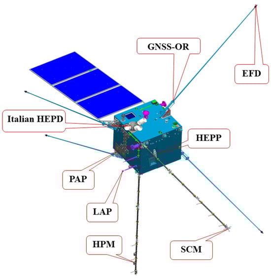
Figure 1.
The layout of the payloads onboard CSES-01.
According to the results of the in-flight commission test, data validation, and data quality assessment through comparison with multisource observations, we confirmed that most of the payloads are working stably in-orbit, providing high-accuracy and reliable data products, except for PAP and TBB [22]. The PAP was contaminated after launch, leading to lower absolute values of Ni and larger Vi than expected at this altitude of the ionosphere. Fortunately, after comprehensive analysis through comparison with other missions, we found that the relative values of Ni and Vi are stable and have the capability of describing the ionospheric variation features similar to those observed from other missions. It is recommended that the relative values of PAP be carefully used for scientific applications [31]. The middle band (400 MHz) of TBB malfunctioned after launch, and the data products of TBB have not yet been completely assessed [32]; thus, it was not included in this study. The status of each scientific payload onboard CSES-01 is summarized in Table 1.

Table 1.
The status of the payloads onboard CSES-01.
The standard data products of CSES-01 are classified into five levels, see Zhima et al. [21] for details. Among these, the Level-2 standard products are the calibrated physical parameters with the necessary information, including geographic and geomagnetic coordinates, time, altitude, etc., which can be directly applied to scientific applications and shared with the international scientific community through the website (https://www.leos.ac.cn/, accessed on 1 August 2024).
2.2. Data Processing Methods
Based on reliable observations from CSES-01, data processing methods were developed to extract abnormal information related to EQs as objectively as possible. The data preprocessing is performed as follows:
- (1)
- In most cases, only nightside data (ascending orbit) were selected to avoid the significant impact of solar radiation on the ionosphere [33].
- (2)
- Data under disturbed space weather conditions (i.e., |Dst| > 30 nT and Kp > 3) were excluded to eliminate interference caused by space weather [34].
- (3)
- Any artificial interference was minimized by carefully selecting and applying appropriate filtering techniques. For example, the total geomagnetic field data from HPM can be interfered with by TBB signals with at most 30 nT; thus, we developed an algorithm to remove the overlapped disturbances induced by TBB [35].
- (4)
- Data were further extracted within a spatial range of ±10° around the epicenter (latitude/longitude), defined as “the EQ influential zone” according to the empirical equation put forward by Dobrovolsky et al. [14], and within a time window of 25 days before and 5 days after the mainshock based on previous research results [36,37].
After the above data preprocessing steps, the data were applied for further analysis to extract possible anomaly information. Considering the different payloads with different working principles, the different parameters from different payloads have different backgrounds and anomaly features; therefore, different methods were applied and tested to extract seismic anomalies as objectively as possible from each payload for the same EQ case. Then, based on years of data processing and research results, we selected appropriate and effective processing methods for different parameters according to their characteristics and different manifestations [22]. For example, the running quartile method is mainly used for physical values provided by payloads such as LAP, PAP, GOR, and HPM; the difference map is mainly used for payloads including SCM, and EFD in this work. In addition, for the CSES HEPP payload, we mainly used the electron flux comparison method which is a common and effective processing method for energetic particles [38]. Figure 2 shows the flow of data processing.
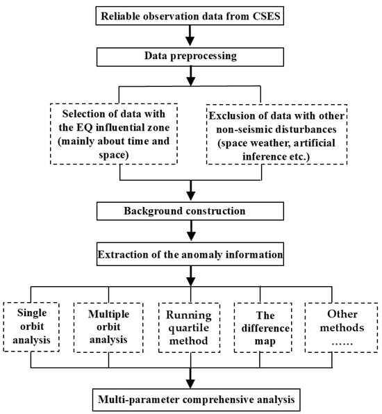
Figure 2.
The flowchart of data processing.
Here, we introduce the three most commonly used methods.
- (1)
- Running quartile method
Firstly, for each EQ event, the current orbits within 25 days before and 5 days after the main shock passing through the EQ influential zone were selected; thus, for each current orbit, we obtained six revisiting orbits within 30 days to build the background trend. Secondly, the running medians (Mb) and interquartile ranges (i.e., IQR, the difference between the third and first quartiles) were computed using the six revisiting orbits. Then, the upper and lower thresholds were computed by the Mb ± n × IQR values, where n is set as values from 1 to 5 depending on the regular features of different physical quantities. Thirdly, the values Mb and Mb ± n × IQR were rebuilt as time sequences and regarded as the background trend. Fourthly, the disturbance amplitude was extracted by comparing the current orbit (Mc) with the background trend values, using the following equation: Mc − (Mb ± n × IQR). Lastly, we normalized the disturbance amplitude as percentages: When the current observation values fall within the upper and lower thresholds, the disturbance amplitude is then set to zero; otherwise, it is set as Mc − (Mb ± n × IQR)/(Mb ± n × IQR).
- (2)
- The difference map
The long-term observations (monthly or yearly data) under quiet space weather conditions were selected to build a global background map with a resolution of 2° (lat) × 2° (lon) grid, which helps depict large-scale ionospheric structure variations [39]. The current global map can be built using the median or mean values for specific parameters routinely every five days (i.e., the revisiting period of the satellite). Then, the regional background map over the EQ influential zone can be extracted from the global background map. After that, the difference map was built by calculating the difference values in each grid between the current map and the background map over the EQ influential area (every five days within 25 days before and 5 days after the mainshock) to depict the abnormal variations during seismic activity.
- (3)
- The particle integration comparison
The HEPP observations within the appropriate time window and inside the EQ influential zone were selected. The electrons were categorized into two energy ranges: 0.1–0.3 MeV and 0.3–3.0 MeV. Then, the electron flux was calculated by integrating it over scattering angles. According to previous research, the variation of electron flux greater than 0.5 orders of magnitude is regarded as anomalous flux relative to the “no-anomalous” period in the same region, which is rated as highly significant [38]. It is noted that only seismic events that occurred away from the South Atlantic Anomaly (SAA) region or the outer radiation belts can be analyzed using the electron flux comparison method.
3. Results
To the observations from different payloads onboard CSES-01, we conducted a comprehensive and retrospective examination for the abnormal phenomena during the global strong shallow EQs. Since its launch in February 2018, by the end of February 2023, CSES-01 completed its five-year lifespan design and is still stably operating in orbit. During its 5-year operation, CSES-01 collected observations, including 66 global strong EQs with a magnitude of Ms ≥ 7 (https://news.ceic.ac.cn/speedsearch.html, accessed on 1 August 2024). According to previous pioneering studies [6,15,36,37], the propagation capability of seismic anomalies from the lithosphere to the ionosphere depends on the magnitude and depth of the EQ. Given that there are rare reports of seismic ionospheric disturbance induced by EQs with a depth ≥ 100 km, this study only focuses on the shallow and strong EQs with a depth ≤ 100 km and Ms ≥ 7 that occurred during CSES-01’s 5-year operation. Figure 3 shows the distribution of the 47 EQs involved in this study.
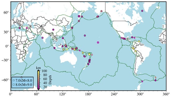
Figure 3.
The distribution of global shallow, strong EQs with a depth ≤ 100 km and Ms ≥ 7 occurred from February 2018 to February 2023.
3.1. An Example of EQ Case Analysis
Here, we take a very significant earthquake event that occurred in Türkiye on February 6 as an example to introduce the process of analyzing seismic ionospheric anomalies.
This strong earthquake included double shocks that occurred consecutively within a day. The first one, with a magnitude of 7.8, occurred at the local time of 4:17 a.m. (1:17 UTC), centered about 70 km from Gaziantep, in Şekeroba (37.15°N, 36.95°E, with a focal depth of 20 km); the second one, with a magnitude of 7.8 occurred 100 km north of the first epicenter, in Ekinözü (38°N, 37.15°E, focal depth 20 km) at the local time of 1:24 pm [40]. This sequence of earthquakes caused widespread damage and resulted in tens of thousands of casualties in Türkiye and Syria. The bilateral rupture propagation of both mainshocks across multiple fault segments was observed [40].
Figure 4 displays the epicenters of the double EQs in Türkiye (red stars) and the EQ influential zone (magenta dashed range), which covers around a 10° (latitude) × 10° (longitude) area, computed using the equation of Dobrovolsky [14]. The orbit trajectories of CSES-01 (blue curves) within this influential zone, spanning from 25 days before to 5 days after the mainshocks, are shown in the enlarged image (the black sector boundary), where the red stars represent the epicenters, and the magenta dashed range shows the influential zone (10° × 10°). The blue curves illustrate the ascending orbit (nightside) trajectories of the CSES-01 satellite.
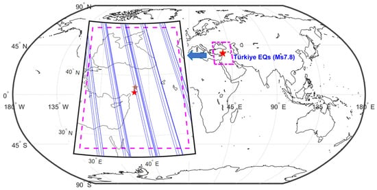
Figure 4.
The orbit trajectories of CSES-01 data selected for the Türkiye EQs on 6 February 2023. The red stars represent the epicenters, and the magenta dashed range shows the potential influential zone (10° × 10°). The blue curves illustrate the ascending orbit (nightside) trajectories of the CSES-01 satellite. The black sector boundary is the boundary of an enlarged image.
By using the running quartile method based on the selected data presented in Figure 4, the variation in electron density (Ne) and oxygen ion density (NO+) from 11 January to 9 February over the EQ influential zone are illustrated in Figure 5. From top to bottom, the panels display the space weather indexes (Kp and Dst), Ne, the variation amplitude (%) of Ne, NO+, and the variation amplitude (%) of NO+. The red vertical lines in all panels mark the mainshock time of the EQ. In the first panel, the blue bars represent the Dst index, and the green curves correspond to the Kp index, while the red horizontal dashed lines represent the value of Kp = 3. In the second and fourth panels, the current variation trend of Ne and NO+ is depicted as blue curves, while the background trends (i.e., median values) are represented by black curves; the upper and lower boundaries are shown as pink curves. In the third and fifth panels, the blue lines represent the change amplitude (%) of Ne and NO+, and the red horizontal dashed lines represent the variation amplitude of 50% and -50% respectively, which are the criteria for identifying possible seismic anomalies of plasma density based on previous research experience [15]. It is observed that an unusual synchronous increase in Ne and NO+ occurred on 27 January (marked by red ellipses, 10 days before the EQ) under quiet space weather conditions, indicating a possible link to the EQ. The other two sets of abnormal increases before the EQ and one increase after the EQ (marked by green rectangles) were primarily associated with space weather conditions, as evidenced by the space weather index presented in the first panel of Figure 5.
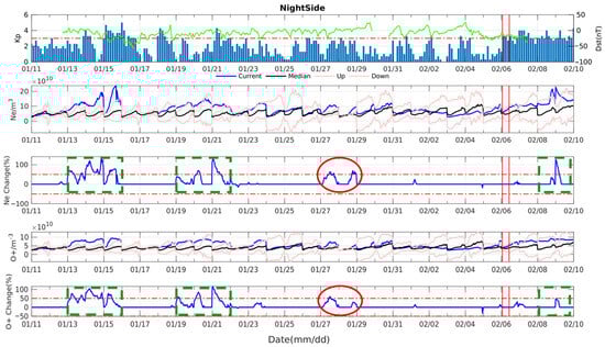
Figure 5.
The disturbances in Ne and NO+ over the influential area of the Türkiye EQ from 11 January to 9 February. From the top panel to the bottom panel: The space weather indexes (Kp and Dst), Ne, the change amplitude (%) of Ne, NO+, and the change amplitude (%) of NO+. The red vertical lines in all panels mark the time of the EQ. In the first panel, the blue bars represent the Dst index, and the green curves correspond to the Kp index, while the red horizontal dashed lines represent the value of Kp = 3. In the second and fourth panels, the current variation trend of Ne and NO+ is depicted as blue curves, while the background trends (i.e., median values) are represented by black curves; the upper and lower boundaries are shown as pink curves. In the third and fifth panels, the blue lines represent the change amplitude (%) of Ne and NO+, and the red horizontal dashed lines represent the disturbance amplitude of 50% and −50% respectively.
We calculated difference maps of the magnetic field above the EQ influential zone every 5 days (matching the recursive period of CSES-01) to extract the magnetic field fluctuations before and after the EQ. Figure 6 displays the difference maps of the magnetic field at the 70 Hz frequency from 11 January to 9 February 2023 around the Türkiye EQs. Panels (a) to (f) represent six revisiting orbit periods, spanning 25 days before and 5 days after the EQ, specifically 11–15 January, 16–20 January, 21–25 January, 26–30 January, 31 January–4 February, and 5–9 February. From the difference maps, it is evident that the Power Spectral Density (PSD) values of the magnetic field exhibited significant enhancement throughout the region during the period from 11 to 15 January (Figure 6a, 20 to 25 days prior to the mainshock) and from 5 to 9 February (Figure 6f, after the mainshock). Given that Kp indexes exceeded 3 during these two periods, the obvious large-scale enhancements are more likely attributed to space weather, which did not appear during other time windows. Apart from these difference maps, a slight enhancement in the southwest of the epicenter (marked by a black arrow) under quiet space weather conditions could be observed in Figure 6e (31 January–4 February), potentially linked to the Türkiye EQ activity. It must be noted that the difference map often appears disturbed, making it challenging to derive reliable seismic information solely based on this method [22].
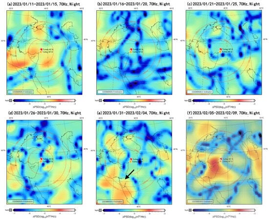
Figure 6.
The difference maps of the magnetic field at the 70 Hz frequency from 11 January to 9 February 2023 around the Türkiye EQ influential area. The epicenters are marked with stars. Figures (a–f) correspond to the periods of 11–15 January, 16–20 January, 21–25 January, 26–30 January, 31 January–4 February, and 5–9 February, respectively. The black arrow in (e) indicates anomalies that may be related to earthquakes.
Figure 7 displays a comparison analysis of the energetic electron flux integration around the Türkiye EQ. Similar to Figure 6, panels (a)–(f) represent six revisiting orbit periods, encompassing 25 days before and 5 days after the EQ. Around 10 days before the EQ, an anomalous electron flux integration increase was observed roughly 700 km north of the epicenter (indicated by the red arrow in Figure 7d). Furthermore, five days before the EQ, another pronounced anomaly appeared around 400 km north of the epicenter (marked by the red arrow in Figure 7e). This seems to indicate that the anomaly appeared 10 days before the EQ, intensified as the EQ approached, and subsequently vanished after the EQ.
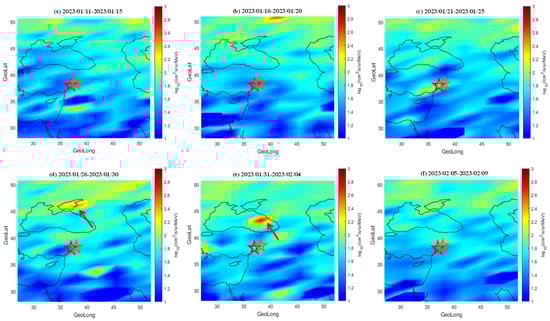
Figure 7.
The comparison maps of integrated energetic electron flux within the 0.1–0.3 MeV during the nightside, centered around Türkiye EQ. The stars denote the epicenters, while the arrows highlight the anomalies. (a–f) correspond to periods of 11–15 January, 16–20 January, 21–25 January, 26–30 January, 31 January–4 February, and 5–9 February, respectively. The red arrows indicate anomalies that may be related to earthquakes.
Based on the examination results of all payloads, we confirmed that anomalies associated with the Türkiye earthquakes were observed by four separate payloads (i.e., LAP, PAP, SCM, and HEPP), all of which emerged within ten days before the mainshock. Compared with other published studies on this Türkiye EQ case, we found that the anomalies indicated by arrows in Figure 6e and Figure 7e coincide with those identified in Figure 6 by Sarlis et al. [41]. These anomalies, with similar timing and position observed in other studies using multiple parameters, could confirm the reliability of the anomaly observed by CSES to a certain extent. Nonetheless, further synchronous evidence from ground-based observations or other observation equipment is imperative to conclusively establish their correlation with seismic precursors.
3.2. Summative Analysis
The summative analysis was conducted based on the results of each EQ case analyzed in the same manner as in Section 3.1. In this work, all 47 shallow EQs with M ≥ 7 and depth ≤ 100 km that occurred from February 2018 to February 2023 were analyzed. It is noted that not all payloads can completely collect observations during all 47 EQs. One reason is that most payloads turn off over latitudes of ±65° [21], so EQs that occurred higher than this latitude will be missed for recording. Only HPM, which operates over the whole latitude range, has the opportunity to collect observations for all 47 EQs. Another reason is that the payload might malfunction or be under experiment coincidentally during the EQ. For example, the recordings of EFD around the equatorial region interfered with the artificial signals from the satellite platform; thus, the recordings from EFD were not qualified for EQs that occurred in this region [22]. As a result, the number of EQs analyzed based on EFD is less than 47. The third reason is that for some payloads, such as GOR, data acquisition depends on the location of the occultation events, so it has less chance to recode EQs.
After careful data selection and examination, we finally collected reliable data for 38 EQ cases from payloads including SCM, LAP, PAP, and HEPP, for 32 EQ cases from GOR and EFD, and for 47 EQs from HPM, as summarized in Table 2 and Figure 8. Table 2 highlights the number of EQs showing certain ionospheric anomalies recorded by at least one payload.
Table 2.
The number of EQs with anomalies compared to all EQ cases analyzed by seven payloads onboard CSES-01.
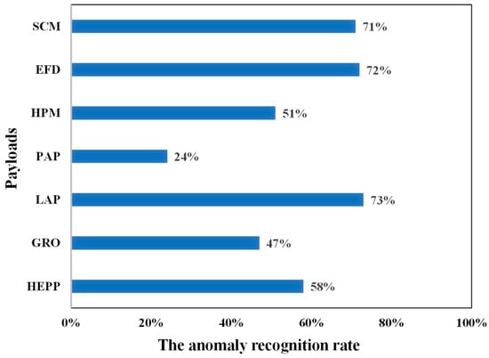
Figure 8.
The anomaly recognition rate to global shallow strong EQs (Ms ≥ 7 and depth ≤ 100 km) of each payload onboard CSES-01.
Based on the results presented in Table 2, the anomaly recognition rates for these analyzed global shallow strong EQs for each payload have been calculated and are depicted in Figure 8. Here, the anomaly recognition rate for each payload is defined as the ratio of the number of EQs with ionospheric anomalies observed to the number of EQs for which that payload has reliable observations. Take the example of SCM: a total of 38 EQs were analyzed, and SCM observations during 27 EQs showed potential seismic-related phenomena; thus, the anomaly recognition rate for SCM is 71% (27/38).
It is evident that LAP, EFD, and SCM exhibit anomaly recognition rates for global shallow strong EQs exceeding 70%, indicating their good detection capability during these seismic events. HEPP, HPM, and GOR register approximately 50% anomaly recognition rates. PAP has a low anomaly recognition rate of 24% due to less qualified data after it became contaminated. It is noteworthy that, despite the detection rate of HPM not being the highest, the anomalies identified by HPM have been deemed more reliable than those from other payloads, according to a predictive experiment we carried out by using space–ground comparative observations in southwest China (unpublished).
Additionally, for each EQ case, we assessed the number of payloads that simultaneously captured the anomalous phenomena, followed by a summative analysis encompassing all 47 strong shallow earthquakes, as shown in Figure 9, where the horizontal axis represents the groups of payloads (set as 1, 2, 3, 4, 5+ payloads) that simultaneously recorded anomalies for the same EQ event, and the vertical axis represents the number of EQs with certain anomalies recorded by different payload groups. The red percentage marks the proportion of the number of earthquakes observed. We conclude the following:
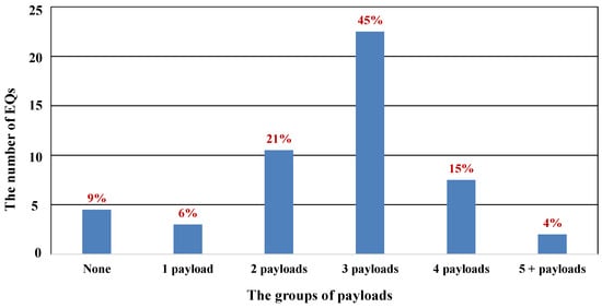
Figure 9.
The proportional distribution of synchronization anomalies from multiple payloads for each earthquake (EQ) case.
- For over 90% of these 47 strong shallow EQs, certain anomalies were captured by at least one payload onboard CSES-01;
- For more than 65% of these 47 strong shallow EQs, two or three payloads onboard CSES-01 could simultaneously record the ionospheric anomalies before the mainshock. Among them, 45% of these EQs exhibited anomalies that were concurrently recorded by three payloads, while about 21% of these EQs displayed anomalies detected simultaneously by two payloads;
- For about 4% of these EQs, five or more payloads recorded disturbances related to the EQs.
In addition, we summarized the most sensitive parameters to EQs of each payload and their respective spatiotemporal distribution characteristics of anomalies, as presented in Table 3.
Table 3.
Seismic-ionospheric anomalies and their spatiotemporal distribution observed by CSES-01.
- (1)
- Regarding electromagnetic fields, anomalies mainly manifest in the ULF and ELF bands. For ionospheric plasma parameters, fluctuations in plasma density are more frequently observed, whereas changes in plasma temperature are less common. The anomalies observed by EFD and SCM are often synchronized in time and position; the anomalies of ionospheric plasma parameters usually appear later than those in the electromagnetic field, while energy particles are closer to the time of EQ occurrence.
- (2)
- The majority of the abnormal variations detected by payloads exhibit positive anomalies, or, in other words, show enhancement phenomena.
- (3)
- The occurrence times of anomalies are predominantly concentrated in three periods: the mainshock day, within 7 days, or 11 to 15 days before the mainshock. Additionally, anomalies in the electromagnetic field are often detected as early as 20–25 days before the EQ.
- (4)
- The spatial distribution of anomalies exhibits an overall tendency to shift toward the equator, but nearly all of the anomalies fall within Dobrovolsky’s radius. Specifically, for EQs occurring in the Northern Hemisphere, anomalies tend to appear in the south of the epicenter, and vice versa in the Southern Hemisphere, though they are not as obvious as those for EQs in the Northern Hemisphere.
4. Conclusions and Discussion
This retrospective study of the CSES-01’s observations during strong shallow EQs shows that the CSES-01 has the capability to detect ionospheric disturbances during seismic activity under quiet space weather, providing a valuable reference for earthquake monitoring from space. The main conclusions are summarized as follows:
- (1)
- The observations from CSES-01 under quiet space weather conditions show that during the majority (over 90%) of the 47 shallow strong EQs (Ms ≥ 7 and depth ≤ 100 km), at least one payload captured certain abnormal signals; during more than 65% of these 47 EQ cases, two or three payloads onboard CSES-01 simultaneously recorded the ionospheric anomalies in multiple physical values; and during about 4% of these EQs, five or more payloads could simultaneously record multiple ionospheric disturbances. Additionally, the larger the magnitude, the more abnormal signals appear across multiple physical values;
- (2)
- The majority of anomalies recorded by different payloads onboard CSES-01 predominantly manifest within one week before or on the mainshock day, or occasionally appear about 11–15 days or 20–25 days before the mainshock;
- (3)
- Typically, the abnormal signals detected by the CSES-01 do not appear directly overhead the epicenter, but rather hundreds of kilometers away from the epicenter, and more preferably toward the equatorward direction;
- (4)
- For the different parameters analyzed in this study, the plasma density from LAP, the electromagnetic field in the ULF band recorded by EFD and SCM, and the energetic electron in the lower energy band from HEPP show a relatively high occurrence of abnormal phenomena during the seismic activity period;
- (5)
- The anomaly recognition rates of seismic-related signals of payloads onboard CSES-01 vary: LAP, EFD, and SCM have the highest anomaly recognition rates, exceeding 70%; HEPP, HPM, and GOR have anomaly recognition rates of approximately 50%; and PAP has a low anomaly recognition rate of 24% due to contamination.
In this study, the time window during which anomalies tend to be observed is relatively regular and consistent with previous studies (e.g., [3,5,6,18]), based on the previous missions (e.g., the DEMETER satellite). However, the precise quantitative spatial locations of the anomalies are difficult to summarize, in most cases, they still fall in Dobrovolsky’s radius (or the magnetic conjugate points), which has been confirmed as the maximum distance from the earthquake epicenter [14,16,17]. The anomalies during the EQ period detected by CSES-01 are not located exactly over the epicenter but mostly away from the epicenter. Many previous studies also confirm that the disturbance does not occur directly above the epicenter but often shifts toward the equatorial direction and may also occur in the magnetic conjugate region [34,42]. According to the LAIC, there are several coupling channels (e.g., [8,16,17,18,43,44]). For example, in terms of the electric field, it is believed that the electric field caused by earthquakes will deviate toward the equatorial direction when it reaches the ionosphere along the magnetic field lines [16,43]. For the plasma parameters, the vertical ExB drift velocity will also push the anomalies westward due to the overall addition of spatial and seismogenic electric fields in the western area of the conductivity anomaly. For the electromagnetic emissions, the propagation direction is impacted by the variations in conductivity and the ambient magnetic field [16,17,44]. These features indicate that different physical parameters with different propagation mechanisms may cause anomalies to appear in different directions. Thus, it is challenging for this retrospective study to compare multiple types of physical parameters in a standard way.
It should be noted that the anomaly recognition rates of all payloads in this work are preliminary. There are several reasons leading to the different recognition rates of the payloads. Firstly, the sample size of EQs for each payload is different and also not sufficient to make a quantitative analysis. Secondly, the working performance of payloads varies. For example, the inherent issues within the PAP itself result in inaccurate observations and, thus, a low anomaly recognition rate. Thirdly, due to the different working principles (or working mechanisms) of payloads for detecting different physical values, we need to adopt different data processing methods for different types of physical values to extract abnormal signals. This leads to differences in the anomaly extraction results. Lastly, the correlation between different parameters and earthquakes varies. For example, some parameters are more easily affected by seismogenic processes. As our knowledge accumulates through increasing observations and experience in the future, it is anticipated that data processing methods will evolve, and the accuracy and objectivity of the anomaly detection rates from the payloads will improve.
Although CSES-01 can record abundant ionospheric anomalies during strong and shallow EQs, and the common characteristics of these anomalies have been summarized and confirmed by numerous previous studies [3,8,19,45], there is still a significant gap between seismic monitoring and effective forecasting at present due to high rates of missed detections and false alarms. This situation can be attributed to several reasons.
- (1)
- The lack of high-resolution observation capability
The recursive period of CSES-01 is 5 days, meaning it passes over a fixed location once every 5 days, and the minimum distance between two orbits is approximately 5° in the longitude direction (i.e., 500 km at the equator). However, both the time resolution of 5 days and the spatial resolution of 5° are inadequate for capturing all the seismic anomalies in the ionosphere. There is a possibility that the satellite may completely miss flying over the areas where seismic anomalies appear, or just fly past the edge of the disturbance area [23]. After the launch of CSES-02 in the future, which will operate concurrently with CSES-01, the revisiting orbit period will be reduced to 2–3 days, which effectively improves the spatiotemporal resolution of CSES observations. However, it is still not enough for the accurate real-time acquisition of seismic anomaly signals. Therefore, by combining the long-term observation data from the ground-based equipment and similar satellites in orbit at the same time, stereoscopic observation could be constructed, and more data from the lithosphere–atmosphere–ionosphere can be obtained to compensate for the lack of spatial and temporal resolution of existing satellite observations.
- (2)
- The challenges due to the different data processing methods lead to different anomaly extraction criteria
As mentioned in Section 2, we employed efficient processing methods according to the data characteristics for different parameters; therefore, the magnitude of abnormal changes in different parameters may vary significantly, making it challenging to establish a quantitative relationship among different parameters. It is difficult to accurately identify disturbances related to EQ from numerous disturbances present in satellite observations, relying solely on variations of a single parameter. Methods and criteria that consider the coupling relationships among different parameters are crucial for capturing the EQ-related disturbances from various parameters. In the future, incorporating AI and big data technologies could delve deeper into the data for information and further enhance our ability to obtain these relationships.
- (3)
- The limitation of extracting weak seismic signals under a strong and varying space background
With the advent of strong solar activity years in the 25th solar cycle, solar flares, magnetic storms, and other events are on the rise, leading to frequent disturbances in ionospheric observation data, thus forming a complex and continuously dynamic ionospheric background environment. The ionospheric anomalies caused by the EQ preparation process are notably weak and localized when compared to this complex changing background, making it extremely challenging to effectively identify seismic anomalies from those caused by space weather disturbances. In this way, we need to obtain more observational data on the lithosphere, atmosphere, and ionosphere. The evolution process of different events can be mastered with the help of observational data from different spheres, to understand the relationship between different variations of ionospheric parameters throughout the whole evolution process, and to better distinguish the changes in observational data caused by different events.
- (4)
- The shortcomings and complexity of the LAIC mechanism
The lithosphere–atmosphere–ionosphere Coupling (LAIC) mechanism provides a potential theoretical explanation for the ionospheric disturbance during the EQ preparation process [17,18]. However, in most cases, models may fail to provide quantitative support for seismic anomalies because the simulation results often differ by several orders of magnitude when compared to actual observations or ground experiment results [43,46]. Consequently, given the complexity of seismic genesis, further understanding and research on LAIC are necessary until the process of LAIC is well understood. Therefore, more data are needed for practice and testing, thus leading to a better understanding of the coupling mechanism.
So far, estimating the risk of potential EQs is still a challenge, particularly in accurately predicting the three key elements of impending EQs (i.e., time, location, and magnitude). Satellite-based observation offers advantages such as all-weather, global coverage, short periods, high efficiency, and strong dynamics, which play an important role in the study of EQ occurrence mechanisms, EQ monitoring and prediction, EQ disaster prevention, and emergency rescue operations [1]. Through satellite observation, the monitoring range can be expanded globally, so that more EQ cases as well as more abundant data can be obtained. Earthquake monitoring and prediction extend beyond the field of geophysics; it is necessary to enhance the spatiotemporal resolution of satellite data through the subsequent series of CSES satellites and constellation plans, integrate the ground-based electromagnetic, deformation, fluid, and gravity observational data, and combine disciplines such as seismology, geodesy, and geochemistry, etc. By adopting a comprehensive approach to “hunt” for EQ precursors, we can overcome the scientific challenge of EQ prediction. Further detailed research in this field is needed in the future.
Author Contributions
Conceptualization, R.Y., Z.Z. (Zeren Zhima), J.H. and J.L.; Methodology, R.Y., Y.Y., Q.W., J.H., D.L., Z.Z. (Zhenxia Zhang), W.C., S.X. and H.L.; Software, R.Y., Y.Y., Q.W., J.H., D.L., Z.Z. (Zhenxia Zhang), W.C., S.X., H.L., W.P. and L.W.; Investigation, R.Y., Z.Z. (Zeren Zhima), Y.Y., Q.W., J.H., D.L., Z.Z. (Zhenxia Zhang), W.C., S.X., H.L. and J.L.; Data Curation, N.Z., W.L. and Q.T.; Writing—Original Draft, R.Y. and W.P.; Writing—Review and Editing, Z.Z. (Zeren Zhima) and R.Y.; Writing—Formatting modification, W.P.; Resources, Z.Z. (Zeren Zhima); Supervision, Z.Z. (Zeren Zhima), J.H. and J.L. All authors have read and agreed to the published version of the manuscript.
Funding
This work was supported by the National Key R&D Program of China (Grant No. 2023YFE0117300), ISSI/ISSI-BJ (Grant No. 23-583/57), and Dragon 6 cooperation (Grant No. 95437). The CSES data is funded by the China National Space Administration (CNSA) and China Earthquake Administration (CEA).
Data Availability Statement
The data from CSES can be downloaded from the website (https://www.leos.ac.cn/, accessed on 1 August 2024). The solar wind parameters and geomagnetic Kp and Dst indices are provided by the World Data Center for Geomagnetism, Kyoto (https://wdc.kugi.kyoto-u.ac.jp/, accessed on 1 August 2024). The earthquake catalog is provided by the China Earthquake Networks Center (https://news.ceic.ac.cn/speedsearch.html, accessed on 1 August 2024).
Acknowledgments
The successful operation of the CSES is attributed to numerous colleagues both domestically and internationally, who are appreciated by authors for their dedication and intelligence devoted to the CSES mission.
Conflicts of Interest
The authors declare no conflicts of interest.
References
- Zhang, X.; Wang, Y.; He, X. Earthquake Disasters and Seismic Risk Reduction. China Insur. 2022, 2, 35–39. (In Chinese) [Google Scholar]
- Gokhberg, M.; Morgounov, V.; Yoshino, T.; Tomizawa, I. Experimental measurement of electromagnetic emissions possibly related to earthquakes in Japan. J. Geophys. Res. Solid Earth 1982, 87, 7824–7828. [Google Scholar] [CrossRef]
- Kon, S.; Nishihashi, M.; Hattori, K. Ionospheric anomalies possibly associated with M ≥ 6.0 earthquakes in the Japan area during 1998–2010: Case studies and statistical study. J. Asian Earth Sci. 2011, 41, 410–420. [Google Scholar] [CrossRef]
- Sarkar, S.; Choudhary, S.; Sonakia, A.; Vishwakarma, A.; Gwal, A. Ionospheric anomalies associated with the Haiti earthquake of 12 January 2010 observed by DEMETER satellite. Nat. Hazards Earth Syst. Sci. 2012, 12, 671–678. [Google Scholar] [CrossRef]
- De Santis, A.; Marchetti, D.; Pavón-Carrasco, F.J.; Cianchini, G.; Perrone, L.; Abbattista, C.; Alfonsi, L.; Amoruso, L.; Campuzano, S.A.; Carbone, M. Precursory worldwide signatures of earthquake occurrences on Swarm satellite data. Sci. Rep. 2019, 9, 20287. [Google Scholar] [CrossRef] [PubMed]
- He, Y.; Yang, D.; Qian, J.; Parrot, M. Response of the ionospheric electron density to different types of seismic events. Nat. Hazards Earth Syst. Sci. 2011, 11, 2173–2180. [Google Scholar] [CrossRef]
- Yan, R.; Shen, X.; Huang, J.; Wang, Q.; Chu, W.; Liu, D.; Yang, Y.; Lu, H.; Xu, S. Examples of unusual ionospheric observations by the CSES prior to earthquakes. Earth Planet. Phys. 2018, 2, 515–526. [Google Scholar] [CrossRef]
- Pulinets, S.; Boyarchuk, K. Ionospheric Precursors of Earthquakes; Springer: Berlin/Heidelberg, Germany, 2004; p. 288. [Google Scholar]
- Heki, K. Ionospheric electron enhancement preceding the 2011 Tohoku-Oki earthquake. Geophys. Res. Lett. 2011, 38, L17312. [Google Scholar] [CrossRef]
- Sharma, G.; Nayak, K.; Romero-Andrade, R.; Aslam, M.M.; Sarma, K.; Aggarwal, S. low ionosphere density above the earthquake epicentre region of Mw 7.2, El Mayor–Cucapah earthquake evident from dense CORS data. J. Indian Soc. Remote Sens. 2024, 52, 543–555. [Google Scholar] [CrossRef]
- Nayak, K.; López-Urías, C.; Romero-Andrade, R.; Sharma, G.; Guzmán-Acevedo, G.M.; Trejo-Soto, M.E. Ionospheric Total Electron Content (TEC) anomalies as earthquake precursors: Unveiling the geophysical connection leading to the 2023 Moroccan 6.8 Mw earthquake. Geosciences 2023, 13, 319. [Google Scholar] [CrossRef]
- Yadav, K.S.; Vadnathani, R.B.; Goswami, K.R.; Patel, P.M. Anomalous Variations in Ionosphere TEC Before the Earthquakes of 2021 in the Different Parts of the Globe. Trends Sci. 2023, 20, 5169. [Google Scholar] [CrossRef]
- Zhu, F.; Wu, Y.; Zhou, Y.; Lin, J. A statistical investigation of pre-earthquake ionospheric TEC anomalies. Geod. Geodyn. 2011, 2, 61–65. [Google Scholar]
- Dobrovolsky, I.; Zubkov, S.; Miachkin, V. Estimation of the size of earthquake preparation zones. Pure Appl. Geophys. 1979, 117, 1025–1044. [Google Scholar] [CrossRef]
- Han, C.; Yan, R.; Marchetti, D.; Pu, W.; Zhima, Z.; Liu, D.; Xu, S.; Lu, H.; Zhou, N. Study on electron density anomalies possibly related to earthquakes based on CSES observations. Remote Sens. 2023, 15, 3354. [Google Scholar] [CrossRef]
- Hayakawa, M.; Izutsu, J.; Schekotov, A.; Yang, S.-S.; Solovieva, M.; Budilova, E. Lithosphere–atmosphere–ionosphere coupling effects based on multiparameter precursor observations for February–March 2021 earthquakes (M~7) in the offshore of Tohoku area of Japan. Geosciences 2021, 11, 481. [Google Scholar] [CrossRef]
- Pulinets, S.; Ouzounov, D.; Karelin, A.; Davidenko, D. Lithosphere–atmosphere–ionosphere–magnetosphere coupling—A concept for pre-earthquake signals generation. In Pre-Earthquake Processes: A Multidisciplinary Approach to Earthquake Prediction Studies; John Wiley & Sons: Hoboken, NJ, USA, 2018; pp. 77–98. [Google Scholar]
- Sorokin, V.; Hayakawa, M. Generation of seismic-related DC electric fields and lithosphere-atmosphere-ionosphere coupling. Mod. Appl. Sci. 2013, 7, 1–25. [Google Scholar] [CrossRef]
- Parrot, M.; Berthelier, J.-J.; Lebreton, J.-P.; Sauvaud, J.-A.; Santolík, O.; Blecki, J. Examples of unusual ionospheric observations made by the DEMETER satellite over seismic regions. Phys. Chem. Earth Parts A/B/C 2006, 31, 486–495. [Google Scholar] [CrossRef]
- Shen, X.; Zhang, X.; Yuan, S.; Wang, L.; Cao, J.; Huang, J.; Zhu, X.; Piergiorgio, P.; Dai, J. The state-of-the-art of the China Seismo-Electromagnetic Satellite mission. Sci. China Technol. Sci. 2018, 61, 634–642. [Google Scholar] [CrossRef]
- Zhima, Z.; Dapeng, L.; Xiaoying, S.; Yanyan, Y.; Shufan, Z.; Rui, Y.; Zhenxia, Z.; He, H.; Dehe, Y.; Jie, W. Current status and scientific progress of the Zhangheng-1 satellite mission. Rev. Geophys. Planet. Phys. 2022, 54, 455–465. [Google Scholar]
- Zhima, Z.; Yan, R.; Lin, J.; Wang, Q.; Yang, Y.; Lv, F.; Huang, J.; Cui, J.; Liu, Q.; Zhao, S. The possible seismo-ionospheric perturbations recorded by the China-Seismo-Electromagnetic Satellite. Remote Sens. 2022, 14, 905. [Google Scholar] [CrossRef]
- Zheng, L.; Yan, R.; Parrot, M.; Zhu, K.; Zhima, Z.; Liu, D.; Xu, S.; Lv, F.; Shen, X. Statistical research on seismo-ionospheric ion density Enhancements observed via DEMETER. Atmosphere 2022, 13, 1252. [Google Scholar] [CrossRef]
- Shen, X.; Zhang, X. The development in seismo-ionospheric coupling mechanism. Prog. Earthq. Sci 2022, 52, 193–202. [Google Scholar]
- Cao, J.; Zeng, L.; Zhan, F.; Wang, Z.; Wang, Y.; Chen, Y.; Meng, Q.; Ji, Z.; Wang, P.; Liu, Z. The electromagnetic wave experiment for CSES mission: Search coil magnetometer. Sci. China Technol. Sci. 2018, 61, 653–658. [Google Scholar] [CrossRef]
- Huang, J.; Lei, J.; Li, S.; Zeren, Z.; Li, C.; Zhu, X.; Yu, W. The Electric Field Detector (EFD) onboard the ZH-1 satellite and first observational results. Earth Planet. Phys. 2018, 2, 469–478. [Google Scholar] [CrossRef]
- Li, X.; Xu, Y.; An, Z.; Liang, X.; Wang, P.; Zhao, X.; Wang, H.; Lu, H.; Ma, Y.; Shen, X. The high-energy particle package onboard CSES. Radiat. Detect. Technol. Methods 2019, 3, 45–55. [Google Scholar] [CrossRef]
- Lin, J.; Shen, X.; Hu, L.; Wang, L.; Zhu, F. CSES GNSS ionospheric inversion technique, validation and error analysis. Sci. China Technol. Sci. 2018, 61, 669–677. [Google Scholar] [CrossRef]
- Liu, C.; Guan, Y.; Zheng, X.; Zhang, A.; Piero, D.; Sun, Y. The technology of space plasma in-situ measurement on the China Seismo-Electromagnetic Satellite. Sci. China Technol. Sci. 2019, 62, 829–838. [Google Scholar] [CrossRef]
- Zhou, B.; Yang, Y.; Zhang, Y.; Gou, X.; Cheng, B.; Wang, J.; Li, L. Magnetic field data processing methods of the China Seismo-Electromagnetic Satellite. Earth Planet. Phys. 2018, 2, 455–461. [Google Scholar] [CrossRef]
- Liu, D.; Zeren, Z.; Huang, H.; Yang, D.; Yan, R.; Wang, Q.; Shen, X.; Liu, C.; Guan, Y. The ionospheric plasma perturbations before a sequence of strong earthquakes in Southeast Asia and Northern Oceania in 2018. Remote Sens. 2023, 15, 5735. [Google Scholar] [CrossRef]
- Shen, X.; Zong, Q.-G.; Zhang, X. Introduction to special section on the China Seismo-Electromagnetic Satellite and initial results. Earth Planet. Phys. 2018, 2, 439–443. [Google Scholar] [CrossRef]
- Cao, J.; Yang, J.; Yuan, S.; Shen, X.; Liu, Y.; Yan, C.; Li, W.; Chen, T. In-flight observations of electromagnetic interferences emitted by satellite. Sci. China Ser. E Technol. Sci. 2009, 52, 2112–2118. [Google Scholar] [CrossRef]
- Liu, J.; Huang, J.; Zhang, X. Ionospheric perturbations in plasma parameters before global strong earthquakes. Adv. Space Res. 2014, 53, 776–787. [Google Scholar] [CrossRef]
- Yang, Y.; Zhou, B.; Hulot, G.; Olsen, N.; Wu, Y.; Xiong, C.; Stolle, C.; Zhima, Z.; Huang, J.; Zhu, X. CSES high precision magnetometer data products and example study of an intense geomagnetic storm. J. Geophys. Res. Space Phys. 2021, 126, e2020JA028026. [Google Scholar] [CrossRef]
- Marchetti, D.; Zhu, K.; Yan, R.; Zhima, Z.; Shen, X.; Chen, W.; Cheng, Y.; Fan, M.; Wang, T.; Wen, J. Ionospheric Effects of Natural Hazards in Geophysics: From Single Examples to Statistical Studies Applied to M5. 5+ Earthquakes. Proceedings 2023, 87, 34. [Google Scholar]
- Němec, F.; Santolík, O.; Parrot, M. Decrease of intensity of ELF/VLF waves observed in the upper ionosphere close to earthquakes: A statistical study. J. Geophys. Res. Space Phys. 2009, 114, A04303. [Google Scholar] [CrossRef]
- Wang, L.; Zhang, Z.; Zhima, Z.; Shen, X.; Chu, W.; Yan, R.; Guo, F.; Zhou, N.; Chen, H.; Wei, D. Statistical Analysis of High–Energy Particle Perturbations in the Radiation Belts Related to Strong Earthquakes Based on the CSES Observations. Remote Sens. 2023, 15, 5030. [Google Scholar] [CrossRef]
- Zhima, Z.; Hu, Y.; Piersanti, M.; Shen, X.; De Santis, A.; Yan, R.; Yang, Y.; Zhao, S.; Zhang, Z.; Wang, Q. The seismic electromagnetic emissions during the 2010 Mw 7.8 Northern Sumatra Earthquake revealed by DEMETER satellite. Front. Earth Sci. 2020, 8, 572393. [Google Scholar] [CrossRef]
- Petersen, G.M.; Büyükakpinar, P.; Vera Sanhueza, F.O.; Metz, M.; Cesca, S.; Akbayram, K.; Saul, J.; Dahm, T. The 2023 Southeast Türkiye seismic sequence: Rupture of a complex fault network. Seism. Rec. 2023, 3, 134–143. [Google Scholar] [CrossRef]
- Sarlis, N.V.; Skordas, E.S.; Christopoulos, S.-R.G.; Varotsos, P.K. Identifying the Occurrence Time of the Destructive Kahramanmaraş-Gazientep Earthquake of Magnitude M 7.8 in Turkey on 6 February 2023. Appl. Sci. 2024, 14, 1215. [Google Scholar] [CrossRef]
- Li, M.; Parrot, M. Statistical analysis of the ionospheric ion density recorded by DEMETER in the epicenter areas of earthquakes as well as in their magnetically conjugate point areas. Adv. Space Res. 2018, 61, 974–984. [Google Scholar] [CrossRef]
- Hegai, V.; Kim, V.; Liu, J. On a possible seismomagnetic effect in the topside ionosphere. Adv. Space Res. 2015, 56, 1707–1713. [Google Scholar] [CrossRef]
- Kuo, C.; Huba, J.; Joyce, G.; Lee, L. Ionosphere plasma bubbles and density variations induced by pre-earthquake rock currents and associated surface charges. J. Geophys. Res. Space Phys. 2011, 116, A10317. [Google Scholar] [CrossRef]
- Liu, J.-Y.; Chen, Y.; Chuo, Y.; Chen, C.-S. A statistical investigation of preearthquake ionospheric anomaly. J. Geophys. Res. Space Phys. 2006, 111, A05304. [Google Scholar] [CrossRef]
- Denisenko, V. Estimate for the strength of the electric field penetrating from the Earth’s surface to the ionosphere. Russ. J. Phys. Chem. B 2015, 9, 789–795. [Google Scholar] [CrossRef]
Disclaimer/Publisher’s Note: The statements, opinions and data contained in all publications are solely those of the individual author(s) and contributor(s) and not of MDPI and/or the editor(s). MDPI and/or the editor(s) disclaim responsibility for any injury to people or property resulting from any ideas, methods, instructions or products referred to in the content. |
© 2024 by the authors. Licensee MDPI, Basel, Switzerland. This article is an open access article distributed under the terms and conditions of the Creative Commons Attribution (CC BY) license (https://creativecommons.org/licenses/by/4.0/).