Abstract
Unmanned aerial vehicles (UAVs) have become essential tools with diverse applications across multiple sectors, including remote sensing. This paper presents a trajectory planning method for a team of UAVs aimed at enhancing covert video sensing in uneven terrains and urban environments. The approach establishes a feasible flight zone, which dynamically adjusts to accommodate line of sight (LoS) occlusions caused by elevated terrains and structures between the UAVs’ sensors and the target. By avoiding ‘shadows’—projections of realistic shapes on the UAVs’ operational plane that represent buildings and other obstacles—the method ensures continuous target visibility. This strategy optimizes UAV trajectories, maintaining covertness while adapting to the changing environment, thereby improving overall video sensing performance. The method’s effectiveness is validated through comprehensive MATLAB simulations at both single and multiple UAV levels, demonstrating its ability to prevent LoS occlusions while preserving a high level of camouflage.
1. Introduction
Unmanned aerial vehicles (UAVs) have emerged as indispensable tools with extensive applications spanning various sectors [1,2,3,4]. Among these applications, covert video sensing stands out as a notable example. This application involves the secret tracking and recording of single or multiple targets over vast and dispersed regions using UAVs [1,2,5]. Such covert sensing holds significant value in real-world scenarios, particularly in situations where law enforcement agencies seek to secretly sense or record suspect vehicles or other relevant targets, aiding in the collection of evidence pertaining to suspicious activities [1].
The UAVs must adopt visual camouflage behavior to achieve effective covert video sensing and avoid detection [1,6]. This requires meticulous trajectory planning to conceal the UAVs’ sensing intentions [1,6]. One approach involves operating the UAVs within a carefully designed region that maintains an optimal distance from the target. This region is known as the feasible flight zone, and it allows the UAVs to remain undetected while maintaining a continuous view of the target of interest and capturing it with high-quality video [1]. The zone is continuously adjusted based on the target’s movements, requiring the UAVs to operate within it at all times. To further conceal their sensing intent, the UAVs must execute random flight maneuvers within this zone, avoiding fixed angles and distances relative to the target [1]. This method complicates the target’s ability to detect or recognize the UAVs, ultimately ensuring the success of the covert video sensing mission [1].
However, uneven environments pose significant challenges when planning flight paths using such a method [7,8]. In such scenarios, tall structures or terrains like buildings, hills, and mountains can occlude the line of sight (LoS) between the UAVs’ sensors or cameras and the target, resulting in interruptions in the continuous target observation and complicating effective sensing [8,9,10,11]. This occlusion also could potentially lead to the loss of the target of interest [11]. Hence, for the successful and highly efficient execution of a covert video sensing mission, the employed UAVs must consistently maintain an unobstructed view of the target while evading visual detection [1,2].
In light of this challenge, this paper aims to tackle the issue of LoS occlusion encountered during covert video sensing missions on a single target using multiple UAVs. The primary objective is to devise an effective approach for planning LoS-occlusion-free flight trajectories for multiple UAVs, thereby enabling the highly efficient covert recording of a ground-moving target.
1.1. Contribution
As discussed previously, one approach to planning covert and visually camouflaged trajectories for UAVs is to deploy them within a defined area called the feasible flight zone. Within this zone, the UAVs employ random flying behavior towards the target to achieve the covertness objective of the sensing task [1]. The feasible flight zone encompasses the state space comprising all possible feasible positions for the UAVs, from which waypoints and trajectories can be chosen at each time step to accomplish the sensing objectives. However, in uneven terrain, this approach can encounter challenges. Certain areas within the feasible flight zone might have a blocked LoS between the UAV and the target. Therefore, it is necessary to adjust the feasible flight zone to address these occlusions.
The proposed trajectory planning method in this paper incorporates realistic shapes within the operational plane of the UAVs, representing high and tall structures, as well as terrains such as buildings, hills, and other features commonly found in uneven environments [12]. These shapes determine areas where the target may be occluded from the UAV’s view, referred to as shadows [see Figure 1] [12]. Avoiding these shadows is crucial to preventing LoS occlusions and maintaining the uninterrupted observation of the target over extended periods [12]. Similar considerations regarding shadow design have been made in [12].
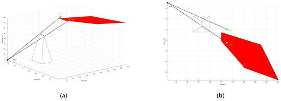
Figure 1.
An illustration of the shadow region (in red) showing how it can occlude the LoS between the UAV sensor and the target. (a) 3D view; (b) 2D view.
In the design of shadows, it should be noted that as the target moves, its position relative to the surrounding terrain shifts. This results in changing shadows that evolve with the target’s movements [12]. Therefore, this paper proposes an approach that adjusts the feasible flight zone online at each time instant, removing parts of the emerging shadows that intersect with it. This creates a new feasible flight zone with a revised state space, ensuring a clear LoS to the target and positioning it outside the shadows.
This paper introduces a novel approach to planning trajectories for multiple UAVs to conduct covert video sensing in urban and uneven terrain environments. The primary contributions of the paper are as follows:
- Construct a specific operational area for UAVs, termed a ‘feasible flight zone’, designed to ensure covert behavior and visual camouflage while sensing the target of interest.
- Propose an approach to adaptively adjust this feasible flight zone in response to intersected shadow regions, representing areas with an occluded LoS due to terrain and structures.
- Update the feasible flight zone at every time step as the target moves.
- Plan collision-free and LoS occlusion-free trajectories for multiple UAVs operating within this feasible flight zone to conduct covert video sensing in uneven environments.
1.2. Related Work
Recent studies have explored the difficulties of using UAVs for the covert video sensing and surveillance of ground targets. The main objective is to explore methods for achieving visual camouflage, enabling UAVs to secretly monitor targets [6]. Various strategies have been developed to achieve this disguise. For example, in studies [1,2], visual camouflage requires consistently altering the UAV’s position to deceive the target [6]. Study [1] alters both the angle and distance between the UAV and the target, while [2] adjusts the UAV’s heading while keeping a constant distance and varying altitude [13].
Other research, such as in [14], explores relative stationarity for visual camouflage, using motion camouflage guidance described by Srinivasan and Davey in [15]. In a related study [16], researchers apply motion camouflage with the additional requirement of maintaining a fixed distance from the target. Motion camouflage has also been applied in other covert monitoring scenarios. For instance, ref. [17] introduces a method using optimal control to create motion camouflage trajectories for UAVs using unicycle motion models [13].
Most prior studies have concentrated on utilizing a single UAV for covert sensing and monitoring, neglecting investigations into visual camouflage with multiple UAVs [13]. Additionally, challenges such as LoS occlusion in uneven terrain for covert sensing missions have yet to be explored.
Numerous attempts have been made to address the issue of LoS occlusion in uneven terrains. Most of them have primarily addressed scenarios where targets are aware of video sensing. Several studies have introduced various methods to avoid these occlusions and ensure the continuous sensing and coverage of targets. For instance, authors in [18] developed a path planning algorithm using model predictive control for multiple UAVs tracking ground vehicles across rugged terrain. Their approach effectively mitigates LoS obstructions caused by uneven terrain, thereby ensuring uninterrupted video surveillance [18].
In addition to this, studies such as [19,20] have also investigated the collaborative use of UAVs with unmanned ground vehicles (UGVs) to overcome visual obstructions posed by tall obstacles in uneven terrains. Dynamic occupancy grids and Bayesian filtering are utilized in these studies to model the state of the target and continuously update its location probability [19]. Path planning algorithms are then utilized to compute optimal trajectories that maximize the sum of probability of detection within a specified time frame [19].
Moreover, in [12], the authors delineate regions within the UAV’s operational plane, where the UAV loses the LoS with the target as shadows. These shadows exhibit intricate shapes and shift with changes in the target’s position relative to buildings [12]. By avoiding these shadows, the observation duration during target tracking can be extended [12]. They have developed a scalable feedback control strategy for tracking the target, which includes shadow avoidance, utilizing a stochastic optimal feedback control framework [12]. Additionally, several other studies, referenced in [9,21,22], have made significant contributions to addressing LoS occlusion in target tracking, further enriching the body of research in this domain.
1.3. Article Organization
This article is organized into several sections. Section 2 details the system model and essential definitions, setting the stage for the problem under investigation. In Section 3, the proposed solution is discussed. Section 4 shows the simulation results, providing an assessment and validation of the proposed approach. The final section discusses conclusions and suggests directions for future research.
2. Materials and Methods
This section outlines the system model and key definitions, introducing the problem addressed in this paper, along with the proposed solution and essential methods used.
2.1. System Model
The investigated system consists of a team comprising communicating UAVs, denoted as . Each UAV is outfitted with a camera and assigned the task of tracking and sensing a single target covertly as it moves along a known route over uneven terrains [13,23]. All UAVs maintain a fixed altitude, denoted as , within the permissible deployment range, and operate within a plane parallel to the ground plane . The horizontal coordinates for any UAV at any given time within the time frame are denoted as . Here, the interval encompasses the entire duration of the UAVs’ covert video sensing mission [13,23]. The dynamics of any UAV are modeled using the kinematic model, neglecting wind disturbances, as follows [24]:
In (1), the variable indicates the orientation of UAV relative to the x-axis, with values ranging between 0 and 2π, measured counterclockwise [1,13,23]. We use to represent the linear speed of UAV , restricted to the range , and for its angular speed, which falls within . These speed variables are limited by constants and , reflecting the maximum achievable linear and angular speeds based on the UAVs’ mobility characteristics in practice [1,13,23]. During maneuvers involving a non-zero angular velocity , the turning radius of UAV is computed by the formula [1,13,23].
To prevent collisions between any two UAVs, it is crucial to adhere to the following constraint at any time:
where a consistent minimum safe separation distance, denoted as between any pair of UAVs and (where ), which move according to the kinematic model described in (1), must be satisfied. Failure to meet the condition in (2) during movement requires implementing measures to avoid potential collisions, such as those described in [13,23]. Note that and other safety constraints must be carefully chosen to align with the specifications and design requirements of the UAVs, as detailed in [25,26].
All UAVs share a common mission, which is conducting covert video sensing on a single moving target in uneven terrains. These complex terrains are particularly prevalent in urban environments, characterized by numerous tall buildings, walls, and narrow roads [27,28]. Such obstacles can occlude the LoS between the UAV and the target, impeding effective monitoring or recording [9,10,11].
The monitored target travels along a specified road within an urban environment. The target’s position at any time is denoted by [1,13,23]. The angle of the target’s movement, measured counterclockwise from the x-axis, is denoted as [1,13,23]. Estimation and prediction algorithms can be employed to assess and predict target positions [29]. For practical considerations, it is assumed that when a target is recorded and seen by a UAV, its position and velocity can be determined using image processing techniques through its camera [29]. Whenever the target is not viewed, its current position can be predicted from previously available measurements [29]. Here, the stability of the UAVs’ cameras is assumed to be guaranteed through the use of a gimbal [1,13,23].
Consequently, by continuously tracking the target’s movement along a specified path, it becomes possible to predict its trajectory into the future for a designated duration, denoted as [1,13,23]. Thus, starting from any initial time , a prediction of the target’s position, , is assumed to be available for the time interval within [1,13,23]. With the known information of the route and the current target position, determining its movement direction at any given moment becomes straightforward [1,13,23].
Let us construct an approximated model of the uneven terrain region and its elevated structures, which collectively form the operational environment of our target. This study is specifically focused on a category of highly uneven terrains, as detailed in [10]. Let us define the subset as a polygon with vertices, serving as our bounded area of interest for target monitoring [10]. Within , there exist smaller, non-overlapping, and distinct polygons denoted as , where , each defined by its unique vertices [10]. Additionally, within each of these polygons, there are corresponding polygons denoted as , possessing an equivalent number of vertices to their respective counterparts [10]. We assume that all these polygons are convex in shape. Every and its corresponding together form a polytope [10]. In this configuration, each forms the foundational base of its associated polytope, while represents its upper surface [10]. Furthermore, each polytope is presumed to consist of side faces, denoted as , where . Each of these side faces forms a convex quadrilateral with one side originating from and the opposite side from [see Figure 2] [10]. It is worth mentioning that may not necessarily align parallel to the ground plane , as depicted in Figure 2. Additionally, we assume they are not perpendicular to it [10].
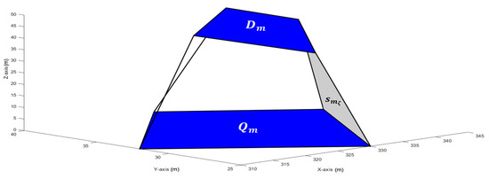
Figure 2.
An illustration of the design of polytope , demonstrating the base face , the top face , and the side [10].
Any and and their corresponding collectively constitute , referring to polytope , representing a distinct tall terrain or structure from a diverse array such as buildings or walls [10]. The 3D coordinates of the edges and corners of each are available and provided as , where denotes a distinct index for each point in the sequence. It is important to note that, in order to prevent UAVs from colliding with the terrain, a safety constraint must be adhered to. This constraint is defined as follows:
where denotes the minimum distance between UAV and the highest point of the terrain, , and is a given positive constant [10]. Furthermore, it is presumed that the remaining areas of polygon , excluding the regions , maintain a relatively flat terrain [10].
This paper assumes that comprehensive environmental data, including ground terrain positions, structures configurations, and altitude variations, are readily available [22]. This assumption is regarded as reasonable, as databases typically include data on significant regional terrains within operational areas [22].
The core of the mission involves covert video sensing, requiring all UAVs to operate within a designated area, known as the feasible flight zone at any given time , as depicted in Figure 3. The design of this feasible zone was initially proposed in [1]. This zone is crucial for ensuring UAVs can maneuver in an undetected way by the target while keeping the target within the UAVs’ field of view [1]. Positioned directly behind the target, it lies between the distances and from the target’s horizontal position in the operational plane at height . indicates the minimum distance UAVs can approach without being detected by the target, while represents the maximum distance from which UAVs can observe the target with satisfactory quality [1]. Moreover, this zone is entirely encompassed within the corresponding annulus specified by an angle , which is then used in conjunction with the target’s heading to derive two additional angles, and . These angles delineate the boundaries of the feasible flight zone, forming arcs that completely enclose it, as illustrated in Figure 3 [1].
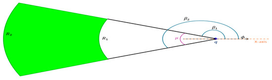
Figure 3.
A demonstration of the feasible flight zone.
Given the predictions of the target position for every and parameters , , , , and , determining the feasible flight zone for any instant is currently straightforward. Hence, for any UAV i, it is required to adhere to the following constraint [1]:
where is the feasible flight zone with the target located at [1].
In various situations, accurately estimating the future location of a target can be challenging, potentially impacting the feasible flight zone for UAVs. We propose the reasonable assumption that prediction uncertainty is bounded at each time slot [1]. This assumption is justified by the realistic limitations on the target’s speed. Consequently, adjusting the design of the feasible flight zone becomes crucial to accommodate uncertainties in target prediction [1].
In (5), the process of determining the feasible flight zone transitions from relying on precise predictions to utilizing approximate ones is completed, employing estimated regions instead of exact coordinates [1]. At any given time , the region is employed to compute the feasible flight zone for any point within it [1]. Consequently, for the effective monitoring of any point within the region, it is essential to calculate the feasible flight zone by intersecting the zones associated with all points within . This revised feasible flight area is denoted as , and each UAV is required to operate within this zone consistently [1,13,23].
Since the mission emphasizes covertness, selecting the right colors for the employed UAVs enhances their visual camouflage. Appropriate colors allow objects to blend into their surroundings, reducing the likelihood of detection [30,31]. By carefully matching the UAVs’ colors to specific environments, their chances of avoiding detection improve, increasing their ability to stay concealed during covert video sensing and boosting overall mission performance. In this paper, the UAVs are equipped with colors that blend seamlessly into uneven terrains, further assessing and improving their camouflage effectiveness.
2.2. Shadow Design and LoS Occlusion Avoidance
As previously explained, the purpose of establishing the feasible flight zone is to maintain an optimal distance between the UAVs and the target, ensuring they are neither too close nor too far [1,13,23]. Within this zone, the UAVs maintain the target within their field of view and can record it with acceptable quality, while remaining concealed [1]. This designated flight zone serves as the state space encompassing all potential UAV positions at any given time [1]. Each UAV can select an optimal position within this feasible flight zone to achieve the main objective of the mission and plan a covert, collision-free trajectory. However, high structures such as buildings, mountains, hills, and other terrain features in uneven environments can block the LoS to the target, potentially resulting in the loss of the target of interest, as illustrated in Figure 1 [9,10,11].
Before we delve into the shadow design, let us examine whether any UAV , at any given instant and any position within the feasible flight zone in (5), maintains an unobstructed LoS to the target in the presence of high structures or terrain. To achieve this, we analyze the straight-line segment connecting any position of the UAV , where , within the feasible flight zone, to the 3D predicted target position at that particular instant [11]. This relationship can be expressed as follows [11]:
where , and is a free number. Assessing whether the UAV and the target maintain an unobstructed LoS at a specific moment involves identifying intersections between the line segment connecting their positions and obstacles that could potentially occlude the LoS, such as tall buildings or mountains [11]. If any intersections are found, it indicates that there is a blocked LoS to the target. Conversely, if no intersections are identified, we can confirm that there is a clear LoS to the target. With the necessary environmental data on hand, confirming a clear LoS between any position within the feasible flight zone and the target is straightforward in real-world applications [11].
Figure 4 illustrates that despite selecting UAVs’ positions within the feasible flight zone in (5) based on an objective function aimed at creating covert paths, all UAVs experience a blocked LoS to the target. This situation could result in losing track of the target, potentially leading to mission failure [9,10,11]. Thus, it is clear that not all states or positions within the feasible flight zone in (5) are viable. While some positions offer better concealment, they may still suffer from an occluded LoS. Addressing this challenge forms the core focus of this paper, aiming to exclude non-viable positions with the occluded LoS from the feasible flight zone. This ensures that the objective function can generate optimal UAV paths from the remaining positions with a clear LoS to the target.
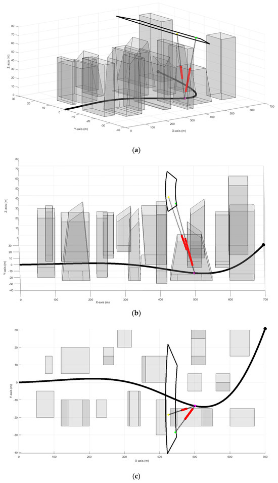
Figure 4.
A demonstration of LoS blockage between UAVs and the target, despite optimal positioning for covert behavior. Red dots indicate blocked LoS. (a,b) are 3D views; (c) is a 2D view.
To exclude non-viable positions with an occluded LoS to the target from the feasible flight zone, adjustments must be made to the calculation process of the feasible flight zone. This involves accounting for regions within the UAVs’ operational plane where the LoS is occluded, thereby excluding them from the feasible flight zone. These regions correspond to realistic projections of tall structures or terrain within the operational region, termed as shadows. Within these areas, UAVs lack a LoS to the target [12]. These shadows constantly change with each time step due to the target’s movement relative to surrounding tall structures and terrain [12]. Consequently, these terrain-induced shadows are dynamic, evolving with the target’s motion (refer to Figure 5). Moreover, these shadows may overlap, forming complex and interconnected shapes [12].
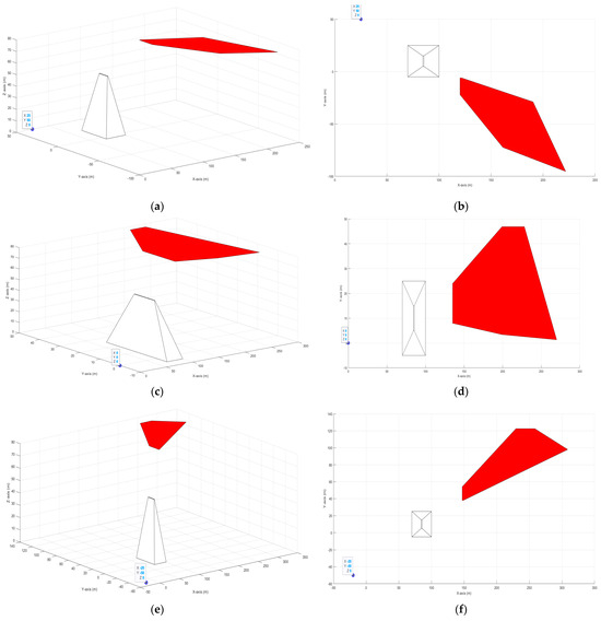
Figure 5.
An illustration shows how the terrain shadow changes with the target’s movement. Each row represents a target position: the first column (a,c,e) shows 3D views of the target (blue circle) and terrain shadow (red area), while the second column (b,d,f) provides corresponding 2D views.
To begin, it is crucial to note that in this paper, the trajectories of the UAVs are periodically planned and computed over multiple time steps within a designated future time frame [1,13,23]. This time frame represents the period in the future when the target position is predictable. It is discretized into intervals with a sampling interval . The time period is segmented into slots of equal duration, where [1]. At each time slot (where ), the continuous-time variables of UAV —, , , and —as well as the target’s variables and , are discretized. They are represented discretely as , , , , , and , respectively [1,13,23]. Subsequently, the system model (1) for UAV is now represented in its discretized form as follows [1,13,23]:
Since we are working in discrete time, we will compute the shadows of all existing terrains and integrate them into the calculation of the new feasible flight zone at the start of each time slot.
Understanding the design of shadows entails recognizing that convex objects, such as those proposed to represent the uneven terrains in this paper, maintain their convexity through perspective projection [12,32]. This approach is practical and can be applied when a 3D map of an uneven area is available [12]. At any time slot , the calculation of the shadow cast by a single structure or terrain onto the operational plane at height , with the target positioned at coordinates [see Figure 6], begins by establishing the vector connecting the target with the points as follows [12]:
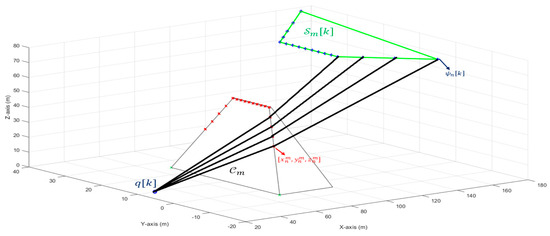
Figure 6.
An illustration showing how the shadow of a terrain is constructed.
Consequently, the vector intersects the plane at the point [12]:
Given that terrain points near the ground correspond to very distant points in the plane, we selectively consider terrain points above a defined minimum height, denoted as , ensuring that for all [12]. This consideration enhances the method’s scalability to the number of terrains and their varying heights. After computing for all pertaining to , we identify the convex hull of the points to depict its shadow, as depicted in Figure 6 [12]. Subsequently, we construct another set comprising subsets , each delineating the shadow of for .
Everything is now in place to modify the feasible flight zone defined in (5) to account for the shadows within the UAVs’ operational plain . These shadows are excluded from the feasible flight zone at each time slot. Let denote the feasible flight zone defined by at time slot . The new feasible flight zone at instant can be represented as the set difference between and the union of all the other shadow regions , . Hence, the new feasible flight zone that any UAV must fly within at any slot is represented as follows:
Equation (10) defines a new feasible flight zone comprising only positions that maintain a clear LoS to the target throughout every time slot.
2.3. Objective Function
The primary issue addressed in this paper involves planning visually camouflaged trajectories for multiple UAVs. The proposed approach employs a method involving random flight patterns within the feasible flight zone to obscure the UAVs’ video sensing intentions towards the target [1,13,23]. Additionally, the energy efficiency of the UAVs’ batteries is crucial, as high energy consumption can significantly reduce their lifespan [1]. Therefore, the objective function formulated for this problem incorporates two key factors: the disguising performance of the UAVs and the energy efficiency of the resulting trajectories.
To achieve the first factor, it is essential to adopt a measure that quantifies the UAV’s concealment or disguising performance effectively. This measure assesses how much the UAV changes its direction and distance from the target over time, combining derivatives of both the UAV-target angle and distance [1]. This quantification is crucial for evaluating the effectiveness of the disguise [1]. Given the involvement of multiple UAVs in this study, the disguising measure for UAV is described as follows [1,13,23]:
Here, is a given positive constant (). represents the angle between UAV and the target (UAV-target angle), measuring the angular difference between the direction of the line connecting UAV and the target and the target’s horizontal direction angle [1,13,23]. Similarly, represents the distance between UAV and the target (UAV-target distance), defined as the Euclidean distance in the horizontal plane between UAV and the target [1,13,23]. The following equations are used for UAV to calculate and [1,13,23]:
Given the positions of the UAVs and the target, measurements for (12) and (13) related to metric (11) can be performed in the field at each time step, ensuring effective observation and validation in practical scenarios. Maximizing the disguising measure described in (11) is crucial for effectively concealing each UAV, such as UAV in this scenario [1,13,23].
This involves each UAV making frequent and significant adjustments to its distance and angle relative to the target at each time step, thereby reducing its exposure to the target view [1].
Having set out to quantify the visual camouflage challenge for each UAV initially, the subsequent objective is to optimize the energy efficiency of their flight paths. In practice, each UAV’s battery capacity is limited, so minimizing energy consumption is crucial to extending their operational lifespan [1]. In this study, the length of each UAV’s trajectory is seen as a measure of its energy consumption [1,13,23]. Therefore, each UAV is responsible for achieving the following objective in planning its flight trajectory [1,13,23]:
By combining these two objectives in (14) and (15), we can form the main objective function to be solved as follows:
where is a weighting factor [1,13,23]. The discretized form of Equation (16) is as follows:
2.4. Problem Statement
Now, with provided parameters , , , , , , , , , , and initial conditions for each UAV, the problem to be addressed is to plan trajectories for UAVs that move according to system (1). These trajectories must minimize the objective function (16) subject to constraints (2), (3), and (10).
2.5. Proposed Solution
The problem is addressed with a decentralized approach, where each UAV independently employs an online trajectory planning method to generate optimal trajectories based on (16). We utilize the Dynamic Programming (DP) method to solve this optimization problem, subject to constraints (1), (2), and (10). DP is chosen for its ability to handle the complexities of the problem, such as nondifferentiability and nonconvexity issues in the second part of the objective function (16). Predicting the target’s motion for the complete video sensing period adds difficulty; hence, we suggest an online DP-based approach that periodically updates each UAV’s trajectory based on short-term predictions over a future time horizon . Each UAV plans its trajectory for the next slots, where [1,13,23].
The process initiates by designating the current time slot as the outset, referred to as stage zero [1,13,23]. At this outset, UAV calculates control inputs, denoted as and , where varies from to . These inputs are selected to minimize Equation (17), ensuring the subsequent position remains within [1,13,23]. Utilizing model (7) and the computed control inputs, in conjunction with the initial position and heading at stage for each UAV, enables the determination of their position and heading throughout each successive time step across the next slots [1,13,23]. This process delineates the optimal flight paths for each UAV throughout the duration .
At stage zero, using the predicted target’s position and heading for the next slots, the feasible flight zones (10) for each slot are established. These zones are determined based on the position and heading of a single target, as well as considering the terrain’s shadow on the operational plane. These values are consistent for all UAVs at each stage; thus, all UAVs share identical feasible flight zones [13,23]. This zone represents the state space of our system, and at stage for all UAVs, it is denoted as , where . This state space is discretized into a grid, and each UAV’s position at any time slot is represented by a grid point within . This discretization ensures that the state space remains finite at each stage [1,13,23].
Now, each UAV has a cost function:
where this function quantifies the cost incurred when transitioning from any state in to any state in [1,13,23]. The values of and are obtained by using and in Equations (12) and (13), respectively, substituting with [1,13,23]. The values of the control inputs and that facilitate this transition and are used in (18) will be explained later in this section.
We rewrite (18) as to represent the cost of transitioning from the th candidate within to the th candidate within [1,13,23]. Here, and are the control inputs and , respectively, required to make this transition [1,13,23]. For simplicity, let . With these definitions in place, we now have all the necessary components to introduce the DP framework that each UAV employs [1,13,23].
Using the DP method, each UAV computes a local path starting from its initial state and spanning subsequent states. It is important to note that not every state in one stage can transition smoothly to every state in the next stage [1,13,23]. This restriction is based on the maximum distance allowed for UAV movement between states within a single time slot [1,13,23]. Consequently, certain combinations of control inputs and may not be achievable, leading to an infinite transition cost indicated by [1,13,23]. Moreover, as finding the final location of each UAV is unnecessary, we introduce a virtual final state at stage with zero cost [1,13,23].
The minimum cost needed for a segment of UAV ’s local path, from initial state to state in stage , is represented as [1,13,23]. The DP method is used in this manner as in [1,13,23]:
Following the computation of , the final optimal cost can be obtained by the following [1,13,23]:
Initially, this DP algorithm computes the cost of transitioning from the starting states to any state in the next stage. At each subsequent stage, the algorithm updates the minimum subtrajectory cost from the previous stage by adding the cost of moving to the next state [1,13,23]. This iterative process continues until all states in the penultimate stage are processed. At the final stage, the cost is set to 0 for all states, thereby simplifying the calculation in (21) [1,13,23]. In this manner, the algorithm identifies the minimum cost of the optimal trajectory. Subsequently, to form the trajectory, an additional backtracking algorithm is necessary [1,13,23].
After obtaining waypoints for their local paths, each UAV shares these data with the others. When conflicts arise between two or more UAVs, such as overlapping waypoints or insufficient separation, the involved UAVs negotiate to determine which UAV will use the conflicted waypoint and which will need to find a new one [13,23]. The UAVs that must find new waypoints resolve these conflicts by eliminating the conflicted waypoints from their state spaces and using the DP algorithm to find alternative waypoints that optimize the main objective [13,23]. This process continues iteratively until all UAVs have final, unconflicted trajectories that are ready for execution. The negotiation process employs methods similar to those described in references [33,34,35].
Now, to move any UAV from its current position to its new position , we must first find and . These parameters are also essential for computing in (18), which is used to implement the DP method [1,13,23]. One approach to determining and involves initiating the UAV’s rotation, if necessary, from its current position at the start of the time slot. The UAV rotates using either or while traveling at a constant linear speed [1,13,23]. This rotation and linear speed continue until the UAV’s heading is directed towards , a position referred to as the tangent point and denoted by [1,13,23]. Once at the tangent point, the UAV stops rotating and travels in a straight line towards with the same constant linear speed [1,13,23]. This design adheres to UAV kinematics by avoiding sudden movements and sharp turns.
To choose between or for any UAV, we need to determine the turn’s orientation at . The UAV decides to turn left or right based on whether is positioned to the left or right of its current heading angle . This decision is made by calculating the angle , which is measured from the x-axis to the vector in the counterclockwise direction [1,13,23]. The UAV then determines the turning direction by evaluating the angle , which represents the angle between the UAV’s current heading and the direction of , measured counterclockwise [1,13,23]. The turning direction is then determined based on this angle as follows [1,13,23]:
The next step is to find the tangent point and the UAV’s linear speed . The linear speed is used to calculate the turning radius (), while the tangent point is where the UAV’s angular speed becomes zero [1,13,23]. The process begins by introducing a unit vector , oriented perpendicular to the UAV’s heading direction . The center of the UAV’s circular turning path, , is then identified. This center is situated away from the UAV’s position , in the direction indicated by [1,13,23]. We now introduce two vectors: one from the center to (denoted as ) and another from the center to the tangent point (denoted as ) [1,11,21]. Let be the angle between these vectors. The method for calculating is outlined as follows [1,13,23]:
It is important to note that the dot product of the tangent line vector and the vector is zero because these vectors are perpendicular [1,11,21]. Since , , , we can derive the following equation as shown in [1] using (23):
In (24), denotes the angle between the vectors and [1]. This angle varies as a function of [1,13,23]. With , you can rotate the unit vector of counterclockwise to find the unit vector of [1,13,23].
Since , for any UAV can be derived using (23) as follows:
Note that, according to (26), is a function of [1,13,23].
For any UAV, the function below is proposed to determine :
Here, represents the arc length between and . Equation (27) requires UAV to reach at speed by the end of the -th time slot [1,13,23]. With being perpendicular to the UAV’s heading, can be written as . Hence, is represented as follows [1,13,23]:
Based on and , (27) can be expressed as follows [1,13,23]:
With all variables depending on , (29) is simplified to solve only for , which gives the linear speed [1,13,23].
After is calculated, is computed. The feasibility of must then be tested. This involves comparing the direction from to with the UAV’s departure direction at . If these directions are similar, is deemed feasible. If they are not similar, should be replaced with to find an alternative tangent point [1,13,23].
3. Results and Discussion
This section evaluates and discusses the performance of the proposed method based on results generated from computer simulations conducted in MATLAB R2022b. We highlight the effectiveness of the proposed approach in planning unobstructed flight paths for the covert video sensing of a single target moving on an uneven terrain. Additionally, we compare the method proposed in this paper to the approach of [1]. This comparison demonstrates the algorithm’s capability to maintain a continuous and clear LoS between the UAVs and the target, ensuring high-quality video sensing in challenging terrains during covert missions. Furthermore, we illustrate how the algorithm dynamically adjusts the feasible flight zone to avoid emerging shadows, ensuring that no candidate position within this zone has an occluded LoS to the target.
The system model presented in this paper is built in MATLAB, and simulation results for scenarios of covert video sensing missions in uneven terrains are implemented. The system’s parameters are defined as follows: , , , , , , , , and . The weighting factor is determined through iterative testing of the simulations in a way that balances disguising performance, energy efficiency, and speed limits of the UAVs, achieving an optimal trade-off for the study’s objectives.
The target of interest travels along a specified road for 70 slots. The road traverses an uneven environment with tall structures and varied terrains scattered along it [see Figure 7]. These structures and terrains are generated using the model proposed in Section 2 [refer to Figure 2]. In the simulation, each building is independently designed offline by assigning it a random height and number of vertices, forming distinct terrains represented by a set of 3D coordinates , where . All terrains or buildings are then combined to create the uneven environment through which the target moves. The UAVs operate within a feasible flight zone characterized by , , and , with adjustments made using (10) if shadows intersect with this zone.
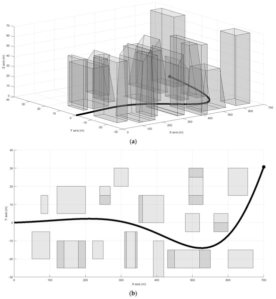
Figure 7.
An illustration of the target movement within the environment: (a) 3D view; (b) 2D view.
In the following subsections, we discuss and analyze the proposed method’s performance from two perspectives: first, using a single UAV, and then, using multiple UAVs.
3.1. Single UAV Performance Analysis
First, we assess the performance of the proposed method using a single UAV. To facilitate this evaluation, we compare it with another method, presented in [1], which adopts a similar approach to covert video sensing but does not account for the challenges posed by LoS occlusion and uneven terrains. The initial position and heading for the UAV are set as and , respectively. Simulation has been executed, and Figure 8 illustrates the trajectories of the UAV engaged in covert video sensing, with the proposed method shown in blue and the method in [1] depicted in red. The figure highlights the effective visual disguising behavior exhibited by the UAV in both methods. Both methods consistently keep the UAV within the feasible flight zone behind the target and enable it to demonstrate random flight patterns through frequent adjustments to the UAV-target angle and distance.
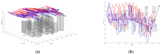
Figure 8.
The UAV trajectories generated by the proposed method (blue) and the method from [1] (red) within the environment: (a) 3D view; (b) 2D view.
To evaluate the video sensing quality of the two methods, we assigned an index, , for each instance where the LoS is either obstructed () or unobstructed (), based on (6). Figure 9 illustrates that the method in [1] encounters numerous occlusions throughout the video sensing mission, in contrast to the proposed method. This increased occlusion can result in a loss of target tracking, leading to lower video sensing quality compared to the proposed method. This outcome is expected, as the method in [1] overlooks the impact of uneven terrains, while the proposed method effectively adjusts to these challenges. This underscores the significance of the proposed method in this paper.
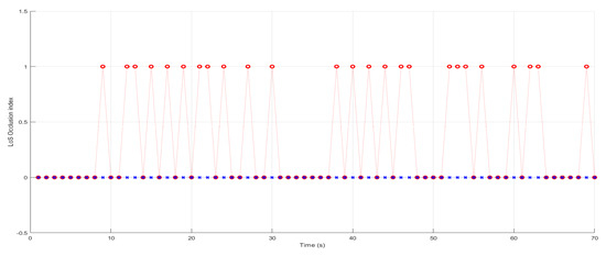
Figure 9.
The LoS occlusion index, where 1 indicates a blocked LoS and 0 indicates a clear LoS. The red circle marks represent the method from [1], while the small blue x-marks represent the proposed method.
Now, to illustrate how the proposed method modifies the feasible flight zone and generates a new zone free from positions that could have blocked the LoS to the target, we will examine one specific time slot, as displaying all 70 slots would be impractical. Figure 10 shows the feasible flight zones for both methods, emphasizing how the proposed method adjusts the zone by accounting for dynamic shadows from tall structures and uneven terrain. In Figure 10a,b, the feasible flight zone of the method in [1] is represented by a solid black line, while the feasible flight zone of the proposed method is indicated by a dotted green line, with shadows shown as light red polygons. It is clear that the feasible flight zone of the proposed method results from eliminating the shadow regions that intersect with the original feasible flight zone generated by the method in [1]. Figure 10c,d demonstrate how the positions within the proposed method’s feasible flight zone ensure an unobstructed LoS to the target, in contrast to the zone generated by the method in [1]. The red dots in Figure 10c,d mark the locations where the LoS is blocked.
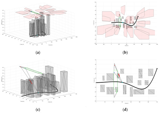
Figure 10.
A demonstration of the feasible flight zone for both methods and how the proposed method accounts for dynamic shadows. Figures (b,d) provide 2D views corresponding to the 3D views shown in figures (a,c).
Figure 11 illustrates the disguising performance of both methods, showing that they maintain comparable levels of performance. Although there are a few instances where the proposed method exhibits a slightly lower level of disguising, these variations are minor and quickly compensated for in the subsequent slot. This temporary decrease in performance is attributed to a narrow and densely packed feasible flight zone caused by the elimination of shadows of a busy, uneven terrain area during that period. Nevertheless, the proposed method consistently avoided LoS occlusion in uneven terrains while maintaining a satisfactory level of disguising performance throughout the mission.
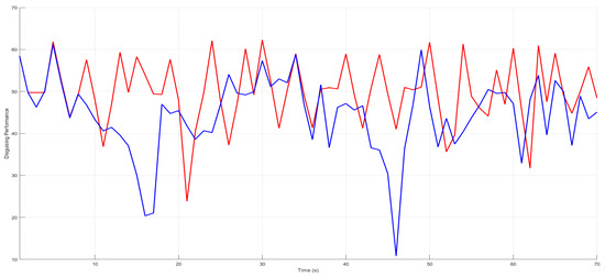
Figure 11.
Disguising performance comparison, with the red line representing the method from [1] and the blue line representing the proposed method.
3.2. Multiple UAVs Performance Analysis
Computer simulations using multiple UAVs are also conducted to assess the performance of the proposed method for the mission. The results are compared from two perspectives: before and after adjusting the feasible flight zone based on the proposed method. Three UAVs were utilized, with the following initial positions and headings: , , , , , and , respectively. The remaining system parameters were consistent with those used in previous simulations. Figure 12 shows the UAV trajectories generated by the proposed method. The UAVs successfully tracked the target while staying within the designated flight area, ensuring a clear LoS. Furthermore, each UAV demonstrated significant camouflage capability, evidenced by notable changes in their positions and orientations relative to the target at each time slot.
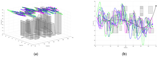
Figure 12.
An illustration depicting the movements of three UAVs (UAV1 in green, UAV2 in magenta, and UAV3 in blue) covertly monitoring a single target (in black): (a) 3D view; (b) 2D view.
Figure 13 demonstrates the LoS occlusion index for each UAV, both before and after accounting for uneven terrains throughout the entire duration of the video sensing mission. Before considering the uneven terrains, all UAVs encountered several blockages in their LoS between their sensors and the target at various times. In contrast, the proposed method effectively maintains a clear LoS for all UAVs throughout the mission, demonstrating improved video sensing quality, as the target was never lost from the LoS of any UAV’s sensor.
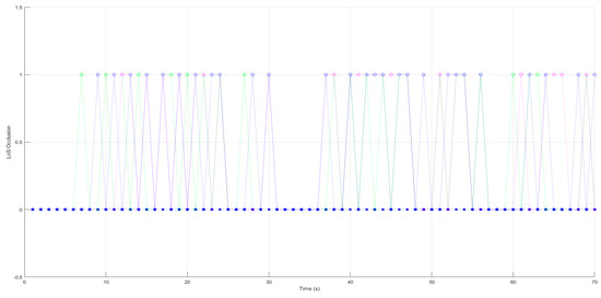
Figure 13.
The LoS occlusion index for multiple UAVs, with 1 indicating a blocked LoS and 0 indicating clear LoS. Circle marks show results before accounting for uneven terrains, while x-marks represent the results of the proposed method.
Figure 14 illustrates the feasible flight zone both before and after accounting for dynamic shadows cast by tall structures and uneven terrain. The figure provides an example from a specific time slot. Figure 14a,b show how the primary feasible flight zone, represented by the black solid line, is modified in the operational plane. The removal of shadows that intersect with the flight zone creates a new feasible flight zone, indicated by the dotted green line. Figure 14c,d demonstrate how the newly generated trajectories within the revised feasible flight zone ensure an unobstructed LoS for each UAV to the target, in contrast to the old feasible flight zone depicted in Figure 14e,f. The red dots in Figure 14e,f mark the locations where the LoS is obstructed.
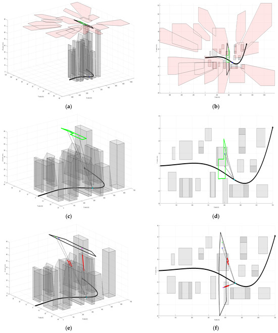
Figure 14.
A demonstration of the feasible flight zone, both before and after accounting for dynamic shadows. Figures (b,d,f) provide 2D views corresponding to the 3D views shown in figures (a,c,e).
Figure 15 displays the disguising performance of each UAV before (represented by dashed lines) and after (represented by solid lines) implementing the proposed method. It demonstrates that the method outlined in this paper does not adversely affect the camouflage performance of multiple UAVs. When compared to a single UAV implementation, there are a few more instances where the disguising performance slightly decreases. This typically occurs when the UAVs traverse areas with a higher density of closely positioned elevated terrain features than previously encountered. Additionally, the need for UAVs to avoid collisions with each other can sometimes compromise their disguising performance, as indicated in [13,23]. However, this reduction does not reach a significant level and is promptly compensated for in subsequent instances. Overall, this underscores the effectiveness of our approach in enabling multiple UAVs to avoid collisions and LoS occlusions, ensuring the creation of safe, covert paths while maintaining an uninterrupted view of the target.
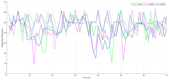
Figure 15.
A comparison of the disguising performance levels of each UAV, with dashed lines representing the performance before the implementation of the proposed method, and solid lines indicating the performance after implementation.
4. Conclusions
In conclusion, this study introduces a novel method for enabling multiple UAVs to conduct covert video sensing in challenging environments such as uneven terrains and urban areas. The method focuses on generating trajectories that maintain a continuous LoS to the target by accounting for the realistic reflection of the obstacles such as buildings, hills, and other terrain features in the operational plane of the UAVs, often referred to as shadows. Avoiding these shadows is crucial to ensure the uninterrupted monitoring of the target. Computer simulations validate the performance of this approach in facilitating UAV collaboration to avoid LoS occlusion, proving effective whether employing a single UAV or multiple UAVs to accomplish the covert sensing mission with continuous visibility of the target of interest. However, there is some disguising performance decrease in extremely uneven terrain parts of the area, which is promptly addressed in subsequent slots. Future research could explore deploying UAVs at varying altitudes rather than a fixed altitude to enhance covertness. Another promising area of study involves investigating the optimal number of UAVs that can be deployed without compromising the secrecy of covert video sensing. Additionally, future studies could focus on developing approaches specifically aimed at enhancing energy efficiency in this context.
Author Contributions
Conceptualization, T.S.A. and A.V.S.; methodology, T.S.A. and A.V.S.; software, T.S.A.; validation, T.S.A.; formal analysis, T.S.A.; investigation, T.S.A.; data curation, T.S.A.; writing—original draft preparation, T.S.A.; writing—review and editing, A.V.S.; visualization, T.S.A.; supervision, A.V.S.; project administration, A.V.S.; funding acquisition, A.V.S. All authors have read and agreed to the published version of the manuscript.
Funding
This work was supported in part by the Australian Research Council. It also received funding from the Australian Government, via grant AUSMURIB000001 associated with ONR MURI grant N00014-19-1-2571.
Data Availability Statement
The data presented in this study are available upon request from the corresponding author, as they are not publicly accessible due to privacy restrictions.
Conflicts of Interest
The authors declare no conflicts of interest.
References
- Huang, H.; Savkin, A.V.; Ni, W. Online UAV Trajectory Planning for Covert Video Surveillance of Mobile Targets. IEEE Trans. Autom. Sci. Eng. 2022, 19, 735–746. [Google Scholar] [CrossRef]
- Hu, S.; Ni, W.; Wang, X.; Jamalipour, A.; Ta, D. Joint Optimization of Trajectory, Propulsion, and Thrust Powers for Covert UAV-on-UAV Video Tracking and Surveillance. IEEE Trans. Inf. Forensics Secur. 2021, 16, 1959–1972. [Google Scholar] [CrossRef]
- Sun, T.; Sun, W.; Sun, C.; He, R. Path Planning of UAV Formations Based on Semantic Maps. Remote Sens. 2024, 16, 3096. [Google Scholar] [CrossRef]
- Tang, G.; Gu, J.; Zhu, W.; Claramunt, C.; Zhou, P. HD Camera-Equipped UAV Trajectory Planning for Gantry Crane Inspection. Remote Sens. 2022, 14, 1658. [Google Scholar] [CrossRef]
- Li, X.; Savkin, A.V. Networked unmanned aerial vehicles for surveillance and monitoring: A survey. Future Internet 2021, 13, 174. [Google Scholar] [CrossRef]
- Hu, S.; Yuan, X.; Ni, W.; Wang, X.; Jamalipour, A. Visual Camouflage and Online Trajectory Planning for Unmanned Aerial Vehicle-Based Disguised Video Surveillance: Recent Advances and a Case Study. IEEE Veh. Technol. Mag. 2023, 18, 48–57. [Google Scholar] [CrossRef]
- Boiteau, S.; Vanegas, F.; Gonzalez, F. Framework for Autonomous UAV Navigation and Target Detection in Global-Navigation-Satellite-System-Denied and Visually Degraded Environments. Remote Sens. 2024, 16, 471. [Google Scholar] [CrossRef]
- Li, Y.; Shi, C.; Yan, M.; Zhou, J. Mission Planning and Trajectory Optimization in UAV Swarm for Track Deception against Radar Network. Remote Sens. 2024, 16, 3490. [Google Scholar] [CrossRef]
- Shaferman, V.; Shima, T. Unmanned aerial vehicles cooperative tracking of moving ground target in urban environments. J. Guid. Control Dyn. 2008, 31, 1360–1371. [Google Scholar] [CrossRef]
- Savkin, A.V.; Huang, H. Proactive deployment of aerial drones for coverage over very uneven terrains: A version of the 3D art gallery problem. Sensors 2019, 19, 1438. [Google Scholar] [CrossRef]
- Huang, H.; Savkin, A.V. Energy-efficient autonomous navigation of solar-powered UAVs for surveillance of mobile ground targets in urban environments. Energies 2020, 13, 5563. [Google Scholar] [CrossRef]
- Munishkin, A.A.; Casbeer, D.W.; Milutinovic, D. Scalable Navigation for Tracking a Cooperative Unpredictably Moving Target in an Urban Environment. In Proceedings of the 2022 IEEE Conference on Control Technology and Applications, CCTA, Trieste, Italy, 23–25 August 2022; Institute of Electrical and Electronics Engineers Inc.: New York, NY, USA, 2022; pp. 484–490. [Google Scholar] [CrossRef]
- Almuzaini, T. Utilizing Multiple UAVs for Covert Aerial Monitoring of a Mobile Target through Decentralized Priority-Based Trajectory Planning. In Proceedings of the 2024 16th International Conference on Computer and Automation Engineering (ICCAE), Melbourne, Australia, 14–16 March 2024; IEEE: New York, NY, USA, 2024; pp. 616–629. [Google Scholar] [CrossRef]
- Savkin, A.V.; Huang, H. Bioinspired Bearing only Motion Camouflage UAV Guidance for Covert Video Surveillance of a Moving Target. IEEE Syst. J. 2021, 15, 5379–5382. [Google Scholar] [CrossRef]
- Srinivasan, M.V.; Davey, M. Strategies for Active Camouflage of Motion. Proc. R. Soc. Lond. Ser. B Biol. Sci. 1995, 259, 19–25. [Google Scholar]
- Strydom, R.; Srinivasan, M.V. UAS stealth: Target pursuit at constant distance using a bio-inspired motion camouflage guidance law. Bioinspir. Biomim. 2017, 12, 055002. [Google Scholar] [CrossRef] [PubMed]
- Rano, I. Direct collocation for two dimensional motion camouflage with non-holonomic, velocity and acceleration constraints. In Proceedings of the IEEE International Conference on Robotics and Biomimetics (ROBIO), Shenzhen, China, 12–14 December 2013; IEEE: New York, NY, USA, 2013; pp. 109–114. [Google Scholar] [CrossRef]
- Savkin, A.V.; Huang, H. Multi-UAV Navigation for Optimized Video Surveillance of Ground Vehicles on Uneven Terrains. IEEE Trans. Intell. Transp. Syst. 2023, 24, 10238–10242. [Google Scholar] [CrossRef]
- Yu, H.; Beard, R.W.; Argyle, M.; Chamerlain, C. Probabilistic Path Planning for Cooperative Target Tracking Using Aerial and Ground Vehicles. In Proceedings of the 2011 American Control Conference, San Francisco, CA, USA, 29 June–1 July 2011; pp. 4673–4678. [Google Scholar]
- Yu, H.; Meier, K.; Argyle, M.; Beard, R.W. Cooperative path planning for target tracking in urban environments using unmanned air and ground vehicles. IEEE/ASME Trans. Mechatron. 2015, 20, 541–552. [Google Scholar] [CrossRef]
- Shaferman, V.; Shima, T. Tracking Multiple Ground Targets in Urban Environments Using Cooperating Unmanned Aerial Vehicles. J. Dyn. Syst. Meas. Control 2015, 137, 051010. [Google Scholar] [CrossRef]
- Kim, J.; Kim, Y. Moving ground target tracking in dense obstacle areas using UAVs. In IFAC Proceedings Volumes; Elsevier: Amsterdam, The Netherlands, 2008; Volume 41, pp. 8552–8557. [Google Scholar] [CrossRef]
- Almuzaini, T. Decentralized Trajectory Planning for Covert Video Surveillance of a Ground-Moving Target Using Multiple UAVs. In Proceedings of the 2024 16th International Conference on Computer and Automation Engineering (ICCAE), Melbourne, Australia, 14–16 March 2024; IEEE: New York, NY, USA, 2024; pp. 653–664. [Google Scholar] [CrossRef]
- Kang, Y.; Hedrick, J.K. Linear tracking for a fixed-wing UAV using nonlinear model predictive control. IEEE Trans. Control Syst. Technol. 2009, 17, 1202–1210. [Google Scholar] [CrossRef]
- Hu, J.; Erzberger, H.; Goebel, K.; Liu, Y. Probabilistic risk-based operational safety bound for rotary-wing unmanned aircraft systems traffic management. J. Aerosp. Inf. Syst. 2020, 17, 171–181. [Google Scholar] [CrossRef]
- Vagal, V.; Markantonakis, K.; Shepherd, C. A new approach to complex dynamic geofencing for unmanned aerial vehicles. In Proceedings of the 2021 IEEE/AIAA 40th Digital Avionics Systems Conference (DASC), San Antonio, TX, USA, 3–7 October 2021; IEEE: New York, NY, USA, 2021; pp. 1–7. [Google Scholar]
- Jakob, M.; Semsch, E.; Pavlíček, D.; Pěchouček, M. Occlusion-aware Multi-UAV Surveillance of Multiple Urban Areas. In Proceedings of the 6th Workshop on Agents in Traffic and Transportation (ATT 2010), 11 May 2010; pp. 59–66. [Google Scholar]
- Uluturk, I.; Uysal, I.; Chen, K.-C. Efficient 3D Placement of Access Points in an Aerial Wireless Network. In Proceedings of the 16th IEEE Annual Consumer Communications & Networking Conference (CCNC), Las Vegas, NV, USA, 11–14 January 2019; pp. 1–7. [Google Scholar]
- Huang, H.; Savkin, A.V.; Li, X. Reactive autonomous navigation of UAVs for dynamic sensing coverage of mobile ground targets. Sensors 2020, 20, 3720. [Google Scholar] [CrossRef]
- Lin, C.J.; Prasetyo, Y.T. A metaheuristic-based approach to optimizing color design for military camouflage using particle swarm optimization. Color Res. Appl. 2019, 44, 740–748. [Google Scholar] [CrossRef]
- Lin, C.J.; Prasetyo, Y.T.; Siswanto, N.D.; Jiang, B.C. Optimization of color design for military camouflage in CIELAB color space. Color Res. Appl. 2019, 44, 367–380. [Google Scholar] [CrossRef]
- Boyd, S.; Vandenberghe, L. Convex Optimization; Cambridge University Press: Cambridge, UK, 2004. [Google Scholar]
- Albaker, B.M.; Rahim, N.A. Unmanned Aircraft Collision Avoidance System Using Cooperative Agent-Based Negotiation Approach. Int. J. Simul. Syst. Sci. Technol. 2010, 11, 1–8. [Google Scholar]
- Vrba, P.; Mařík, V.; Přeučil, L.; Kulich, M.; Šišlák, D. Collision avoidance algorithms: Multi-agent approach. In International Conference on Industrial Applications of Holonic and Multi-Agent Systems; Lecture Notes in Computer Science (including subseries Lecture Notes in Artificial Intelligence and Lecture Notes in Bioinformatics); Springer: Berlin/Heidelberg, Germany, 2007; pp. 348–360. [Google Scholar] [CrossRef]
- Šišlák, D.; Volf, P.; Pěchouček, M. Agent-based cooperative decentralized airplane-collision avoidance. IEEE Trans. Intell. Transp. Syst. 2011, 12, 36–46. [Google Scholar] [CrossRef]
Disclaimer/Publisher’s Note: The statements, opinions and data contained in all publications are solely those of the individual author(s) and contributor(s) and not of MDPI and/or the editor(s). MDPI and/or the editor(s) disclaim responsibility for any injury to people or property resulting from any ideas, methods, instructions or products referred to in the content. |
© 2024 by the authors. Licensee MDPI, Basel, Switzerland. This article is an open access article distributed under the terms and conditions of the Creative Commons Attribution (CC BY) license (https://creativecommons.org/licenses/by/4.0/).