

Satellite-Observed Hydrothermal Conditions Control the Effects of Soil and Atmospheric Drought on Peak Vegetation Growth on the Tibetan Plateau

 , , and
Abstract
1. Introduction
2. Data and Methods
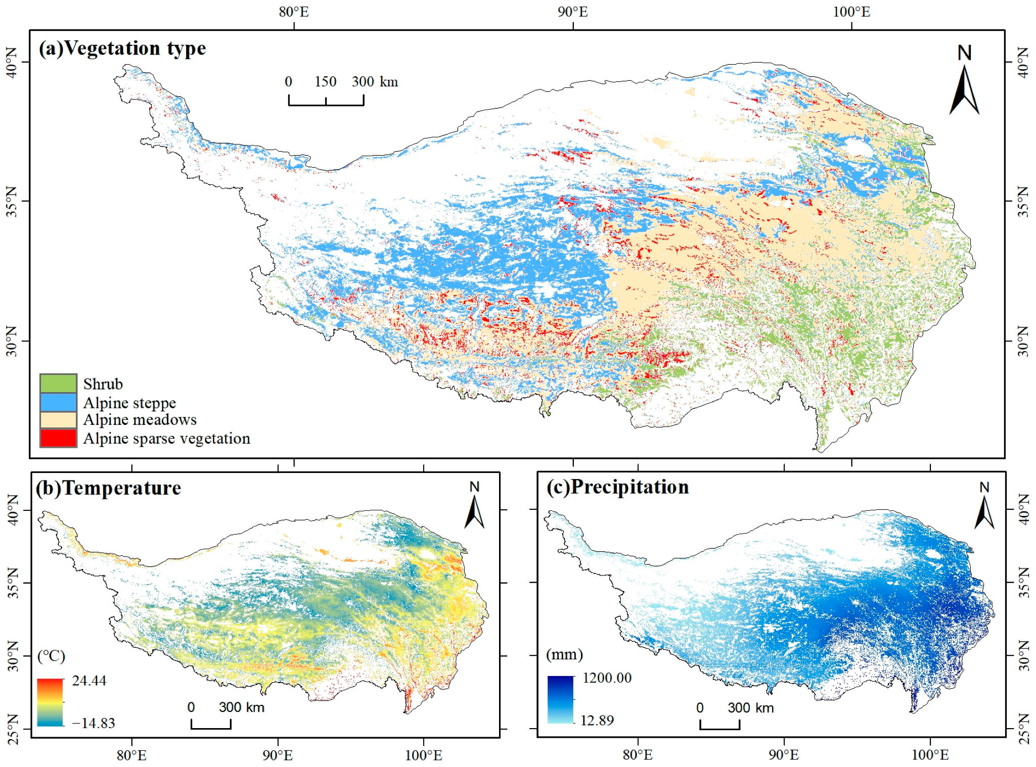
2.1. Study Area
2.2. Data
2.2.1. NDVI Data
2.2.2. GPP Data
2.2.3. Climate Data
2.3. NDVImax and GPPmax Extraction Methods
2.4. Statistical Analysis Strategy
3. Results
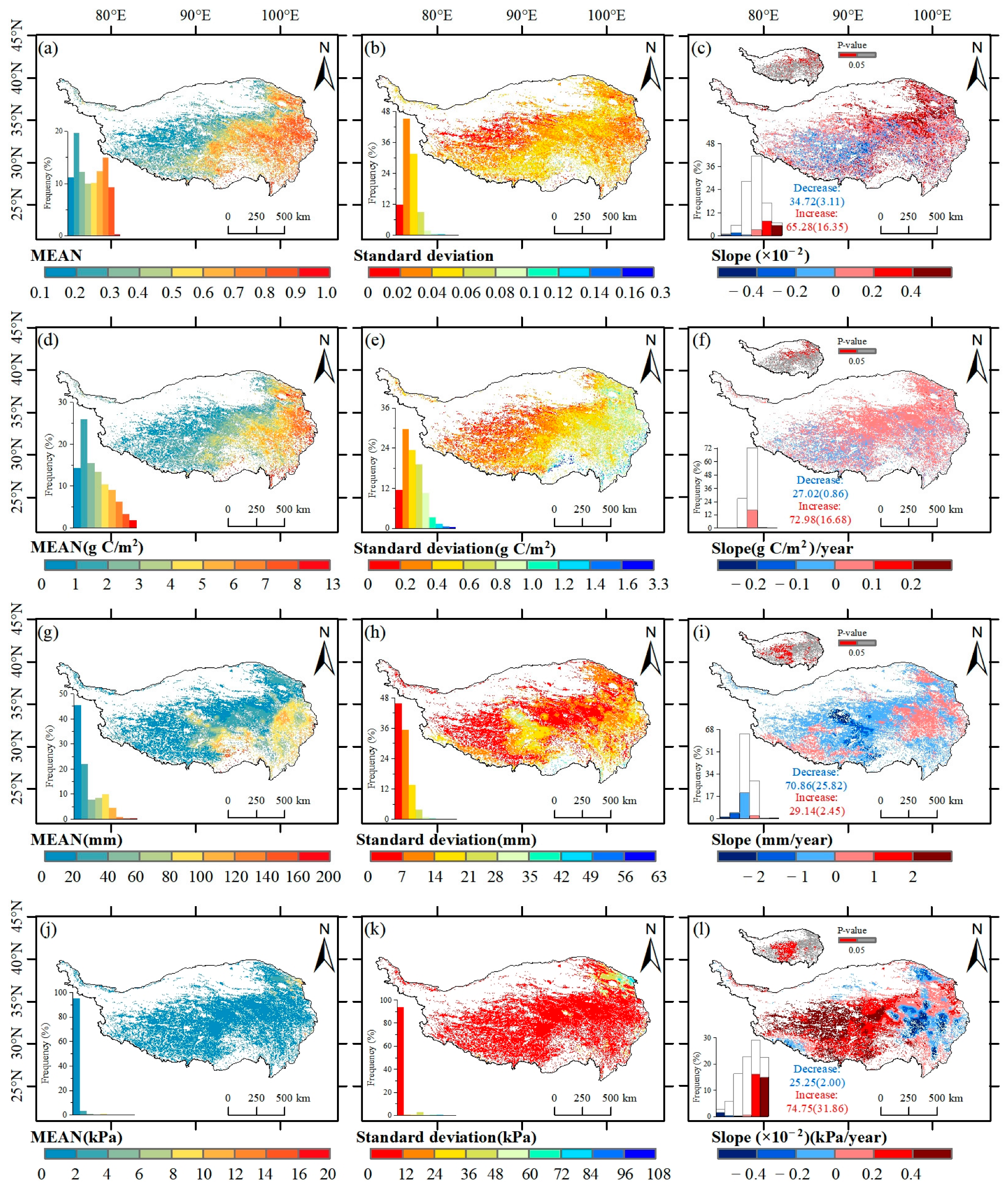
3.1. Spatial and Temporal Patterns of NDVImax and GPPmax
3.2. Spatial and Temporal Patterns of SM and VPD
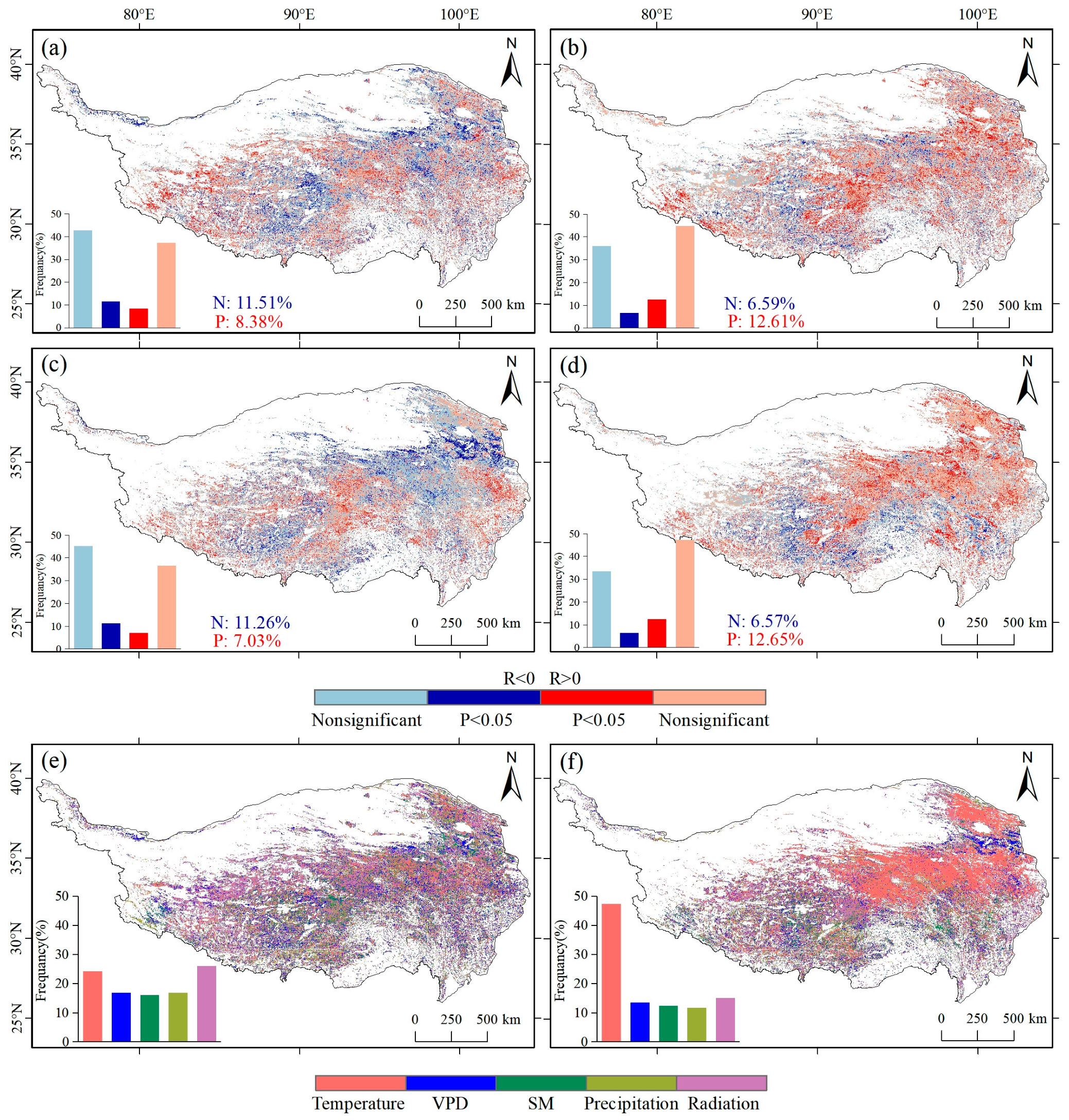
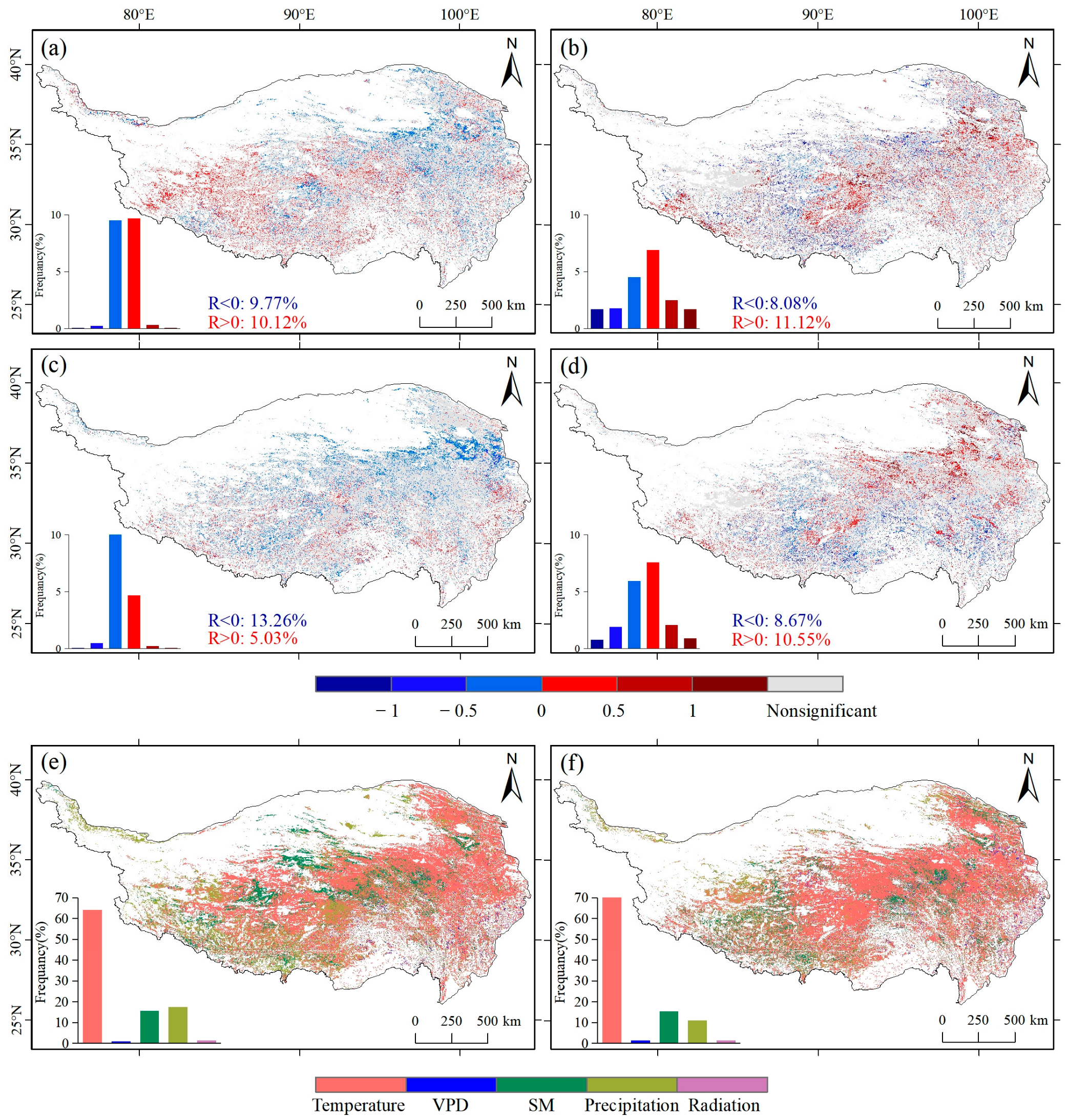
3.3. Response of NDVImax and GPPmax to Climate Data
4. Discussion
4.1. Response of Peak Vegetation Growth to Climate Data
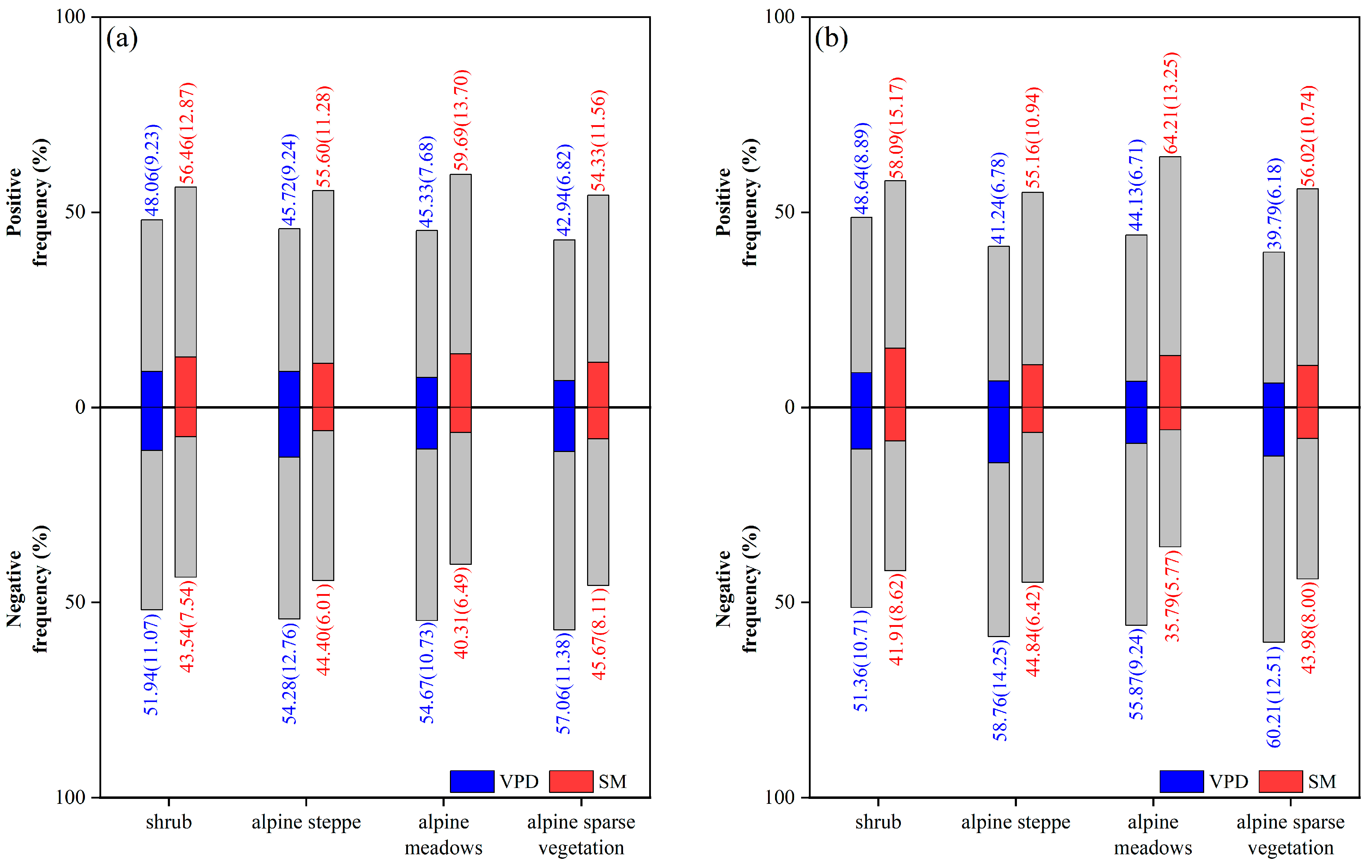
4.2. Performance of Partial Correlation Coefficient on Different Vegetation Types
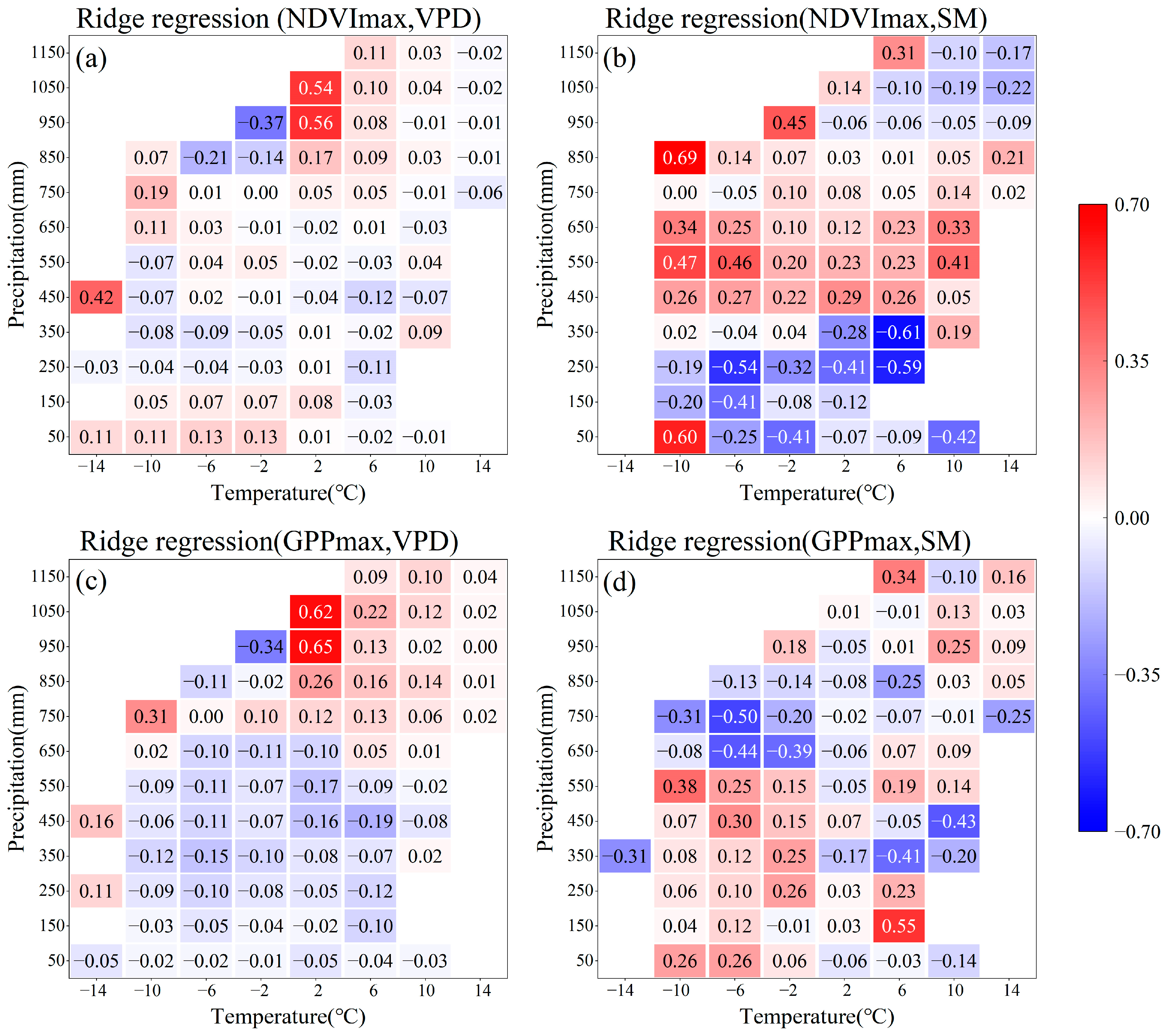
4.3. Response of SM and VPD to Vegetation Growth Peak Under Different Hydrothermal Conditions
4.4. Limitations of the Research
5. Conclusions
Author Contributions
Funding
Data Availability Statement
Conflicts of Interest
References
- Gao, Q.; Guo, Y.; Xu, H.; Ganjurjav, H.; Li, Y.; Wan, Y.; Qin, X.; Ma, X.; Liu, S. Climate change and its impacts on vegetation distribution and net primary productivity of the alpine ecosystem in the Qinghai-Tibetan Plateau. Sci. Total Environ. 2016, 554, 34–41. [Google Scholar] [CrossRef] [PubMed]
- Yao, T.; Bolch, T.; Chen, D.; Gao, J.; Immerzeel, W.; Piao, S.; Su, F.; Thompson, L.; Wada, Y.; Wang, L. The imbalance of the Asian water tower. Nat. Rev. Earth Environ. 2022, 3, 618–632. [Google Scholar] [CrossRef]
- Zhao, D.; Zhu, Y.; Wu, S.; Zheng, D. Projection of vegetation distribution to 1.5 C and 2 C of global warming on the Tibetan Plateau. Glob. Planet. Chang. 2021, 202, 103525. [Google Scholar] [CrossRef]
- Bai, Y.; Guo, C.; Degen, A.A.; Ahmad, A.A.; Wang, W.; Zhang, T.; Li, W.; Ma, L.; Huang, M.; Zeng, H. Climate warming benefits alpine vegetation growth in Three-River Headwater Region, China. Sci. Total Environ. 2020, 742, 140574. [Google Scholar] [CrossRef]
- Wang, Y.; Ma, Y.; Li, H.; Yuan, L. Carbon and water fluxes and their coupling in an alpine meadow ecosystem on the northeastern Tibetan Plateau. Theor. Appl. Climatol. 2020, 142, 1–18. [Google Scholar] [CrossRef]
- Li, H.; Zhu, J.; Zhang, F.; He, H.; Yang, Y.; Li, Y.; Cao, G.; Zhou, H. Growth stage-dependant variability in water vapor and CO2 exchanges over a humid alpine shrubland on the northeastern Qinghai-Tibetan Plateau. Agric. For. Meteorol. 2019, 268, 55–62. [Google Scholar] [CrossRef]
- Saito, M.; Kato, T.; Tang, Y. Temperature controls ecosystem CO2 exchange of an alpine meadow on the northeastern Tibetan Plateau. Glob. Chang. Biol. 2009, 15, 221–228. [Google Scholar] [CrossRef]
- Vanneste, T.; Michelsen, O.; Graae, B.J.; Kyrkjeeide, M.O.; Holien, H.; Hassel, K.; Lindmo, S.; Kapás, R.E.; De Frenne, P. Impact of climate change on alpine vegetation of mountain summits in Norway. Ecol. Res. 2017, 32, 579–593. [Google Scholar] [CrossRef]
- Ahlström, A.; Raupach, M.R.; Schurgers, G.; Smith, B.; Arneth, A.; Jung, M.; Reichstein, M.; Canadell, J.G.; Friedlingstein, P.; Jain, A.K. The dominant role of semi-arid ecosystems in the trend and variability of the land CO2 sink. Science 2015, 348, 895–899. [Google Scholar] [CrossRef]
- Forkel, M.; Carvalhais, N.; Rödenbeck, C.; Keeling, R.; Heimann, M.; Thonicke, K.; Zaehle, S.; Reichstein, M. Enhanced seasonal CO2 exchange caused by amplified plant productivity in northern ecosystems. Science 2016, 351, 696–699. [Google Scholar] [CrossRef]
- Graven, H.; Keeling, R.; Piper, S.; Patra, P.; Stephens, B.; Wofsy, S.; Welp, L.; Sweeney, C.; Tans, P.; Kelley, J. Enhanced seasonal exchange of CO2 by northern ecosystems since 1960. Science 2013, 341, 1085–1089. [Google Scholar] [CrossRef] [PubMed]
- Huang, K.; Xia, J.; Wang, Y.; Ahlström, A.; Chen, J.; Cook, R.B.; Cui, E.; Fang, Y.; Fisher, J.B.; Huntzinger, D.N. Enhanced peak growth of global vegetation and its key mechanisms. Nat. Ecol. Evol. 2018, 2, 1897–1905. [Google Scholar] [CrossRef] [PubMed]
- Xia, J.; Niu, S.; Ciais, P.; Janssens, I.A.; Chen, J.; Ammann, C.; Arain, A.; Blanken, P.D.; Cescatti, A.; Bonal, D. Joint control of terrestrial gross primary productivity by plant phenology and physiology. Proc. Natl. Acad. Sci. USA 2015, 112, 2788–2793. [Google Scholar] [CrossRef] [PubMed]
- Zhu, Z.; Piao, S.; Myneni, R.B.; Huang, M.; Zeng, Z.; Canadell, J.G.; Ciais, P.; Sitch, S.; Friedlingstein, P.; Arneth, A. Greening of the Earth and its drivers. Nat. Clim. Chang. 2016, 6, 791–795. [Google Scholar] [CrossRef]
- Chen, C.; Park, T.; Wang, X.; Piao, S.; Xu, B.; Chaturvedi, R.K.; Fuchs, R.; Brovkin, V.; Ciais, P.; Fensholt, R. China and India lead in greening of the world through land-use management. Nat. Sustain. 2019, 2, 122–129. [Google Scholar] [CrossRef]
- Xu, C.; Liu, H.; Williams, A.P.; Yin, Y.; Wu, X. Trends toward an earlier peak of the growing season in Northern Hemisphere mid-latitudes. Glob. Chang. Biol. 2016, 22, 2852–2860. [Google Scholar] [CrossRef]
- Yang, J.; Dong, J.; Xiao, X.; Dai, J.; Wu, C.; Xia, J.; Zhao, G.; Zhao, M.; Li, Z.; Zhang, Y. Divergent shifts in peak photosynthesis timing of temperate and alpine grasslands in China. Remote Sens. Environ. 2019, 233, 111395. [Google Scholar] [CrossRef]
- Liu, Y.; Wu, C.; Wang, X.; Jassal, R.S.; Gonsamo, A. Impacts of global change on peak vegetation growth and its timing in terrestrial ecosystems of the continental US. Glob. Planet. Chang. 2021, 207, 103657. [Google Scholar] [CrossRef]
- Buermann, W.; Bikash, P.R.; Jung, M.; Burn, D.H.; Reichstein, M. Earlier springs decrease peak summer productivity in North American boreal forests. Environ. Res. Lett. 2013, 8, 024027. [Google Scholar] [CrossRef]
- Gonsamo, A.; Chen, J.M.; Ooi, Y.W. Peak season plant activity shift towards spring is reflected by increasing carbon uptake by extratropical ecosystems. Glob. Chang. Biol. 2018, 24, 2117–2128. [Google Scholar] [CrossRef]
- He, P.; Sun, Z.; Xu, D.; Liu, H.; Yao, R.; Ma, J. Combining gradual and abrupt analysis to detect variation of vegetation greenness on the loess areas of China. Front. Earth Sci. 2021, 16, 368–380. [Google Scholar] [CrossRef]
- Liu, Y.; Wu, C.; Wang, X.; Zhang, Y. Contrasting responses of peak vegetation growth to asymmetric warming: Evidences from FLUXNET and satellite observations. Glob. Chang. Biol. 2023, 29, 2363–2379. [Google Scholar] [CrossRef]
- Du, C.; Chen, J.; Nie, T.; Dai, C. Spatial–temporal changes in meteorological and agricultural droughts in Northeast China: Change patterns, response relationships and causes. Nat. Hazards 2022, 110, 155–173. [Google Scholar] [CrossRef]
- Feng, W.; Lu, H.; Yao, T.; Yu, Q. Drought characteristics and its elevation dependence in the Qinghai–Tibet plateau during the last half-century. Sci. Rep. 2020, 10, 14323. [Google Scholar] [CrossRef] [PubMed]
- Fang, W.; Huang, S.; Huang, Q.; Huang, G.; Wang, H.; Leng, G.; Wang, L.; Guo, Y. Probabilistic assessment of remote sensing-based terrestrial vegetation vulnerability to drought stress of the Loess Plateau in China. Remote Sens. Environ. 2019, 232, 111290. [Google Scholar] [CrossRef]
- Jinsong, W.; Yubi, Y.; Ying, W.; Suping, W.; Xiaoyun, L.; Yue, Z.; Haolin, D.; Yu, Z.; Yulong, R. Meteorological droughts in the Qinghai-Tibet Plateau: Research progress and prospects. Adv. Earth Sci. 2022, 37, 441. [Google Scholar]
- Wu, D.; Hu, Z. Increasing compound drought and hot event over the Tibetan Plateau and its effects on soil water. Ecol. Indic. 2023, 153, 110413. [Google Scholar] [CrossRef]
- Wang, Y.; Fu, B.; Liu, Y.; Li, Y.; Feng, X.; Wang, S. Response of vegetation to drought in the Tibetan Plateau: Elevation differentiation and the dominant factors. Agric. For. Meteorol. 2021, 306, 108468. [Google Scholar] [CrossRef]
- Wu, C.; Peng, J.; Ciais, P.; Peñuelas, J.; Wang, H.; Beguería, S.; Andrew Black, T.; Jassal, R.S.; Zhang, X.; Yuan, W. Increased drought effects on the phenology of autumn leaf senescence. Nat. Clim. Chang. 2022, 12, 943–949. [Google Scholar] [CrossRef]
- Zhao, C.; Brissette, F.; Chen, J. Projection of future extreme meteorological droughts using two large multi-member climate model ensembles. J. Hydrol. 2023, 618, 129155. [Google Scholar] [CrossRef]
- Liu, L.; Gudmundsson, L.; Hauser, M.; Qin, D.; Li, S.; Seneviratne, S.I. Soil moisture dominates dryness stress on ecosystem production globally. Nat. Commun. 2020, 11, 4892. [Google Scholar] [CrossRef] [PubMed]
- Zhou, S.; Williams, A.P.; Berg, A.M.; Cook, B.I.; Zhang, Y.; Hagemann, S.; Lorenz, R.; Seneviratne, S.I.; Gentine, P. Land–atmosphere feedbacks exacerbate concurrent soil drought and atmospheric aridity. Proc. Natl. Acad. Sci. USA 2019, 116, 18848–18853. [Google Scholar] [CrossRef] [PubMed]
- Zhang, W.; Wei, F.; Horion, S.; Fensholt, R.; Forkel, M.; Brandt, M. Global quantification of the bidirectional dependency between soil moisture and vegetation productivity. Agric. For. Meteorol. 2022, 313, 108735. [Google Scholar] [CrossRef]
- Lu, H.; Qin, Z.; Lin, S.; Chen, X.; Chen, B.; He, B.; Wei, J.; Yuan, W. Large influence of atmospheric vapor pressure deficit on ecosystem production efficiency. Nat. Commun. 2022, 13, 1653. [Google Scholar] [CrossRef]
- Zhong, Z.; He, B.; Wang, Y.-P.; Chen, H.W.; Chen, D.; Fu, Y.H.; Chen, Y.; Guo, L.; Deng, Y.; Huang, L. Disentangling the effects of vapor pressure deficit on northern terrestrial vegetation productivity. Sci. Adv. 2023, 9, eadf3166. [Google Scholar] [CrossRef]
- Qi, G.; She, D.; Xia, J.; Song, J.; Jiao, W.; Li, J.; Liu, Z. Soil moisture plays an increasingly important role role in constraining vegetation productivity in China over the past two decades. Agric. For. Meteorol. 2024, 356, 110193. [Google Scholar] [CrossRef]
- Tu, Y.; Wang, X.; Zhou, J.; Wang, X.; Jia, Z.; Ma, J.; Yao, W.; Zhang, X.; Sun, Z.; Luo, P. Atmospheric water demand dominates terrestrial ecosystem productivity in China. Agric. For. Meteorol. 2024, 355, 110151. [Google Scholar] [CrossRef]
- Peng, J.; Wu, C.; Wang, X.; Lu, L. Spring phenology outweighed climate change in determining autumn phenology on the Tibetan Plateau. Int. J. Climatol. 2021, 41, 3725–3742. [Google Scholar] [CrossRef]
- Shen, M.; Zhang, G.; Cong, N.; Wang, S.; Kong, W.; Piao, S. Increasing altitudinal gradient of spring vegetation phenology during the last decade on the Qinghai–Tibetan Plateau. Agric. For. Meteorol. 2014, 189, 71–80. [Google Scholar] [CrossRef]
- Wang, X.; Wu, C.; Liu, Y.; Peñuelas, J.; Peng, J. Earlier leaf senescence dates are constrained by soil moisture. Glob. Chang. Biol. 2023, 29, 1557–1573. [Google Scholar] [CrossRef]
- Abatzoglou, J.T.; Dobrowski, S.Z.; Parks, S.A.; Hegewisch, K.C. TerraClimate, a high-resolution global dataset of monthly climate and climatic water balance from 1958–2015. Sci. Data 2018, 5, 170191. [Google Scholar] [CrossRef] [PubMed]
- Liu, Y.; Wu, C.; Jassal, R.S.; Wang, X.; Shang, R. Satellite observed land surface greening in summer controlled by the precipitation frequency rather than its total over Tibetan Plateau. Earth’s Future 2022, 10, e2022EF002760. [Google Scholar] [CrossRef]
- Shen, M.; Tang, Y.; Chen, J.; Zhu, X.; Zheng, Y. Influences of temperature and precipitation before the growing season on spring phenology in grasslands of the central and eastern Qinghai-Tibetan Plateau. Agric. For. Meteorol. 2011, 151, 1711–1722. [Google Scholar] [CrossRef]
- Yu, F.; Price, K.P.; Ellis, J.; Shi, P. Response of seasonal vegetation development to climatic variations in eastern central Asia. Remote Sens. Environ. 2003, 87, 42–54. [Google Scholar] [CrossRef]
- Liu, W.; Mo, X.; Liu, S.; Lin, Z.; Lv, C. Attributing the changes of grass growth, water consumed and water use efficiency over the Tibetan Plateau. J. Hydrol. 2021, 598, 126464. [Google Scholar] [CrossRef]
- Hoerl, A.E.; Kennard, R.W. Ridge regression: Biased estimation for nonorthogonal problems. Technometrics 1970, 12, 55–67. [Google Scholar] [CrossRef]
- Zhao, Y.; Chen, Y.; Wu, C.; Li, G.; Ma, M.; Fan, L.; Zheng, H.; Song, L.; Tang, X. Exploring the contribution of environmental factors to evapotranspiration dynamics in the Three-River-Source region, China. J. Hydrol. 2023, 626, 130222. [Google Scholar] [CrossRef]
- Golub, G.H.; Heath, M.; Wahba, G. Generalized cross-validation as a method for choosing a good ridge parameter. Technometrics 1979, 21, 215–223. [Google Scholar] [CrossRef]
- Lu, J.; Wang, G.; Li, S.; Feng, A.; Zhan, M.; Jiang, T.; Su, B.; Wang, Y. Projected land evaporation and its response to vegetation greening over China under multiple scenarios in the CMIP6 models. J. Geophys. Res. Biogeosci. 2021, 126, e2021JG006327. [Google Scholar] [CrossRef]
- Piao, S.; Friedlingstein, P.; Ciais, P.; Zhou, L.; Chen, A. Effect of climate and CO2 changes on the greening of the Northern Hemisphere over the past two decades. Geophys. Res. Lett. 2006, 33, L23402. [Google Scholar] [CrossRef]
- Zhao, D.; Zhang, Z.; Zhang, Y. Soil Moisture Dominates the Forest Productivity Decline During the 2022 China Compound Drought-Heatwave Event. Geophys. Res. Lett. 2023, 50, e2023GL104539. [Google Scholar] [CrossRef]
- Liu, L.; Peng, S.; AghaKouchak, A.; Huang, Y.; Li, Y.; Qin, D.; Xie, A.; Li, S. Broad consistency between satellite and vegetation model estimates of net primary productivity across global and regional scales. J. Geophys. Res. Biogeosci. 2018, 123, 3603–3616. [Google Scholar] [CrossRef]
- Oren, R.; Sperry, J.; Katul, G.; Pataki, D.; Ewers, B.; Phillips, N.; Schäfer, K. Survey and synthesis of intra- and interspecific variation in stomatal sensitivity to vapour pressure deficit. Plant Cell Environ. 1999, 22, 1515–1526. [Google Scholar] [CrossRef]
- Stocker, B.D.; Zscheischler, J.; Keenan, T.F.; Prentice, I.C.; Peñuelas, J.; Seneviratne, S.I. Quantifying soil moisture impacts on light use efficiency across biomes. New Phytol. 2018, 218, 1430–1449. [Google Scholar] [CrossRef]
- Williams, A.P.; Allen, C.D.; Millar, C.I.; Swetnam, T.W.; Michaelsen, J.; Still, C.J.; Leavitt, S.W. Forest responses to increasing aridity and warmth in the southwestern United States. Proc. Natl. Acad. Sci. USA 2010, 107, 21289–21294. [Google Scholar] [CrossRef]
- Seneviratne, S.I.; Corti, T.; Davin, E.L.; Hirschi, M.; Jaeger, E.B.; Lehner, I.; Orlowsky, B.; Teuling, A.J. Investigating soil moisture–climate interactions in a changing climate: A review. Earth-Sci. Rev. 2010, 99, 125–161. [Google Scholar] [CrossRef]
- Huber, S.; Fensholt, R.; Rasmussen, K. Water availability as the driver of vegetation dynamics in the African Sahel from 1982 to 2007. Glob. Planet. Chang. 2011, 76, 186–195. [Google Scholar] [CrossRef]
- Grossiord, C.; Buckley, T.N.; Cernusak, L.A.; Novick, K.A.; Poulter, B.; Siegwolf, R.T.; Sperry, J.S.; McDowell, N.G. Plant responses to rising vapor pressure deficit. New Phytol. 2020, 226, 1550–1566. [Google Scholar] [CrossRef]
- Shen, M.; Piao, S.; Dorji, T.; Liu, Q.; Cong, N.; Chen, X.; An, S.; Wang, S.; Wang, T.; Zhang, G. Plant phenological responses to climate change on the Tibetan Plateau: Research status and challenges. Natl. Sci. Rev. 2015, 2, 454–467. [Google Scholar] [CrossRef]
- Li, J.; Wu, C.; Wang, X.; Peng, J.; Dong, D.; Lin, G.; Gonsamo, A. Satellite observed indicators of the maximum plant growth potential and their responses to drought over Tibetan Plateau (1982–2015). Ecol. Indic. 2020, 108, 105732. [Google Scholar] [CrossRef]
- Shen, M.; Piao, S.; Jeong, S.-J.; Zhou, L.; Zeng, Z.; Ciais, P.; Chen, D.; Huang, M.; Jin, C.-S.; Li, L.Z. Evaporative cooling over the Tibetan Plateau induced by vegetation growth. Proc. Natl. Acad. Sci. USA 2015, 112, 9299–9304. [Google Scholar] [CrossRef] [PubMed]
- Yu, H.; Luedeling, E.; Xu, J. Winter and spring warming result in delayed spring phenology on the Tibetan Plateau. Proc. Natl. Acad. Sci. USA 2010, 107, 22151–22156. [Google Scholar] [CrossRef] [PubMed]
- Cong, N.; Shen, M.; Yang, W.; Yang, Z.; Zhang, G.; Piao, S. Varying responses of vegetation activity to climate changes on the Tibetan Plateau grassland. Int. J. Biometeorol. 2017, 61, 1433–1444. [Google Scholar] [CrossRef] [PubMed]
- Wang, X.; Hu, Z.; Zhang, Z.; Tang, J.; Niu, B. Altitude-Shifted Climate Variables Dominate the Drought Effects on Alpine Grasslands over the Qinghai–Tibetan Plateau. Sustainability 2024, 16, 6697. [Google Scholar] [CrossRef]
- Li, X.; Pan, Y. The Impacts of Drought Changes on Alpine Vegetation during the Growing Season over the Tibetan Plateau in 1982–2018. Remote Sens. 2024, 16, 1909. [Google Scholar] [CrossRef]
- Hao, A.; Duan, H.; Wang, X.; Zhao, G.; You, Q.; Peng, F.; Du, H.; Liu, F.; Li, C.; Lai, C. Different response of alpine meadow and alpine steppe to climatic and anthropogenic disturbance on the Qinghai-Tibetan Plateau. Glob. Ecol. Conserv. 2021, 27, e01512. [Google Scholar] [CrossRef]
- Zhang, G.; Zhang, Y.; Dong, J.; Xiao, X. Green-up dates in the Tibetan Plateau have continuously advanced from 1982 to 2011. Proc. Natl. Acad. Sci. USA 2013, 110, 4309–4314. [Google Scholar] [CrossRef]
- Wang, X.; Yi, S.; Wu, Q.; Yang, K.; Ding, Y. The role of permafrost and soil water in distribution of alpine grassland and its NDVI dynamics on the Qinghai-Tibetan Plateau. Glob. Planet. Chang. 2016, 147, 40–53. [Google Scholar] [CrossRef]
- Ganjurjav, H.; Gao, Q.; Gornish, E.S.; Schwartz, M.W.; Liang, Y.; Cao, X.; Zhang, W.; Zhang, Y.; Li, W.; Wan, Y. Differential response of alpine steppe and alpine meadow to climate warming in the central Qinghai–Tibetan Plateau. Agric. For. Meteorol. 2016, 223, 233–240. [Google Scholar] [CrossRef]
- Wang, Y.; Wesche, K. Vegetation and soil responses to livestock grazing in Central Asian grasslands: A review of Chinese literature. Biodivers. Conserv. 2016, 25, 2401–2420. [Google Scholar] [CrossRef]
- Zhang, L.; Guo, H.; Wang, C.; Ji, L.; Li, J.; Wang, K.; Dai, L. The long-term trends (1982–2006) in vegetation greenness of the alpine ecosystem in the Qinghai-Tibetan Plateau. Environ. Earth Sci. 2014, 72, 1827–1841. [Google Scholar] [CrossRef]
- Sun, J.; Qin, X.; Yang, J. The response of vegetation dynamics of the different alpine grassland types to temperature and precipitation on the Tibetan Plateau. Environ. Monit. Assess. 2016, 188, 20. [Google Scholar] [CrossRef] [PubMed]
- Zheng, Z.; Zhu, W.; Zhang, Y. Seasonally and spatially varied controls of climatic factors on net primary productivity in alpine grasslands on the Tibetan Plateau. Glob. Ecol. Conserv. 2020, 21, e00814. [Google Scholar] [CrossRef]
- Liu, Q.; Fu, Y.H.; Zeng, Z.; Huang, M.; Li, X.; Piao, S. Temperature, precipitation, and insolation effects on autumn vegetation phenology in temperate China. Glob. Chang. Biol. 2016, 22, 644–655. [Google Scholar] [CrossRef]
- Shen, M.; Piao, S.; Cong, N.; Zhang, G.; Jassens, I.A. Precipitation impacts on vegetation spring phenology on the Tibetan Plateau. Glob. Chang. Biol. 2015, 21, 3647–3656. [Google Scholar] [CrossRef]
- Wang, X.; Wu, C. Estimating the peak of growing season (POS) of China’s terrestrial ecosystems. Agric. For. Meteorol. 2019, 278, 107639. [Google Scholar] [CrossRef]
- Wu, C.; Chen, J.M.; Desai, A.R.; Lafleur, P.M.; Verma, S.B. Positive impacts of precipitation intensity on monthly CO2 fluxes in North America. Glob. Planet. Chang. 2013, 100, 204–214. [Google Scholar] [CrossRef]
- Fu, Z.; Ciais, P.; Prentice, I.C.; Gentine, P.; Makowski, D.; Bastos, A.; Luo, X.; Green, J.K.; Stoy, P.C.; Yang, H. Atmospheric dryness reduces photosynthesis along a large range of soil water deficits. Nat. Commun. 2022, 13, 989. [Google Scholar] [CrossRef]
- Ma, C.; Wang, X.; Wu, C. Early leaf senescence under drought conditions in the Northern hemisphere. Agric. For. Meteorol. 2024, 358, 110231. [Google Scholar] [CrossRef]

Disclaimer/Publisher’s Note: The statements, opinions and data contained in all publications are solely those of the individual author(s) and contributor(s) and not of MDPI and/or the editor(s). MDPI and/or the editor(s) disclaim responsibility for any injury to people or property resulting from any ideas, methods, instructions or products referred to in the content. |
© 2024 by the authors. Licensee MDPI, Basel, Switzerland. This article is an open access article distributed under the terms and conditions of the Creative Commons Attribution (CC BY) license (https://creativecommons.org/licenses/by/4.0/).
Share and Cite
Qiu, Z.; Tang, L.; Wang, X.; Zhang, Y.; Tan, J.; Yue, J.; Xia, S. Satellite-Observed Hydrothermal Conditions Control the Effects of Soil and Atmospheric Drought on Peak Vegetation Growth on the Tibetan Plateau. Remote Sens. 2024, 16, 4163. https://doi.org/10.3390/rs16224163
Qiu Z, Tang L, Wang X, Zhang Y, Tan J, Yue J, Xia S. Satellite-Observed Hydrothermal Conditions Control the Effects of Soil and Atmospheric Drought on Peak Vegetation Growth on the Tibetan Plateau. Remote Sensing. 2024; 16(22):4163. https://doi.org/10.3390/rs16224163
Chicago/Turabian StyleQiu, Zhengliang, Longxiang Tang, Xiaoyue Wang, Yunfei Zhang, Jianbo Tan, Jun Yue, and Shaobo Xia. 2024. "Satellite-Observed Hydrothermal Conditions Control the Effects of Soil and Atmospheric Drought on Peak Vegetation Growth on the Tibetan Plateau" Remote Sensing 16, no. 22: 4163. https://doi.org/10.3390/rs16224163
APA StyleQiu, Z., Tang, L., Wang, X., Zhang, Y., Tan, J., Yue, J., & Xia, S. (2024). Satellite-Observed Hydrothermal Conditions Control the Effects of Soil and Atmospheric Drought on Peak Vegetation Growth on the Tibetan Plateau. Remote Sensing, 16(22), 4163. https://doi.org/10.3390/rs16224163