Abstract
The spatial resolution (250–1000 m) of the FY-3D MERSI is too coarse for agricultural monitoring at the farmland scale (20–30 m). To achieve the winter wheat yield (WWY) at the farmland scale, based on FY-3D, a method framework is developed in this work. The enhanced deep convolutional spatiotemporal fusion network (EDCSTFN) was used to perform a spatiotemporal fusion on the 10 day interval FY-3D and Sentinel-2 vegetation indices (VIs), which were compared with the enhanced spatial and temporal adaptive reflectance fusion model (ESTARFM). In addition, a BP neural network was built to calculate the farmland-scale WWY based on the fused VIs, and the Aqua MODIS gross primary productivity product was used as ancillary data for WWY estimation. The results reveal that both the EDCSTFN and ESTARFM achieve satisfactory precision in the fusion of the Sentinel-2 and FY-3D VIs; however, when the period of spatiotemporal data fusion is relatively long, the EDCSTFN can achieve greater precision than ESTARFM. Finally, the WWY estimation results based on the fused VIs show remarkable correlations with the WWY data at the county scale and provide abundant spatial distribution details about the WWY, displaying great potential for accurate farmland-scale WWY estimations based on reconstructed fine-spatial-temporal-resolution FY-3D data.
1. Introduction
Winter wheat (WW) is one of the main grain crops in northern China, and the WW growth indices at different growing stages exhibit varying correlations with the final yield (Y). Therefore, continuous time series growth monitoring during the WW growing period (from the regrowth stage to the milk stage) is important for Y estimation [1,2]. Compared with observation data from ground and meteorological stations, remote sensing (RS) technology can detect the continuous spatial distribution of crop growth. A vegetation index (VI), which is calculated based on multispectral reflectance data, is one of the most commonly used methods for estimating crop growth statuses and is characterized by its simplicity and ease of use. Currently, the most commonly employed multispectral VIs for estimating crop growth include the normalized difference vegetation index (NDVI) [3], soil-adjusted vegetation index (SAVI) [4], and enhanced vegetation index (EVI) [5]. The SAVI and EVI were developed based on the NDVI, and they consider soil backgrounds and atmospheric factors, respectively. Relevant studies have shown that the NDVI has a favourable linear or nonlinear relationship with vegetation coverage [6,7], while compared with the NDVI, the SAVI and EVI demonstrate better correlations with the leaf area index [8,9].
Over the past few decades, numerous VI products have been developed using high-temporal-resolution (HTR) satellite sensors, including the NOAA Advanced Very-High-Resolution Radiometer (AVHRR), Terra/Aqua Moderate Resolution Imaging Spectroradiometer (MODIS), and Fengyun-3 (FY-3) Medium Resolution Spectral Imager (MERSI). These products typically exhibit high precision in uniformly distributed farmland areas and can achieve a temporal resolution (TR) as high as 0.5 days. Among them, the FY-3 satellite is a second-generation polar-orbiting solar-synchronous meteorological satellite developed in China. Launched in November 2017, the FY-3 satellite is equipped with a MERSI containing 25 channels, including four visible and near-infrared channels, with a spatial resolution (SR) of 250 m. These channels are essential spectral bands for calculating VI products. The overpass time of FY-3D satellites is approximately 14:00 in the afternoon and the TR of FY-3D can reach 0.5 days. Currently, VIs such as the NDVI and EVI, which are calculated on the basis of satellite sensors such as MODIS, have been widely used in estimating the Y of various crops [10,11]. Johnson et al. [11] estimated the crop Y for barley, spring wheat, and rapeseed on Canadian prairies via the MODIS NDVI and EVI, and the results revealed that in July, the MODIS NDVI can be used to effectively predict the crop Y of the three crops mentioned above and that the combination with the MODIS EVI can further improve the precision of crop Y forecasts. Compared with crop Y estimation models based on VIs during a specific growing period, crop Y estimation models that integrate VIs across multiple growing stages may yield more accurate estimates [12,13,14]. Zhao et al. [12] estimated the winter wheat yield (WWY) in Henan Province based on the MODIS NDVI from March to May, and the results revealed that the multiple linear regression model constructed with the NDVI from multiple months achieved a high Y estimation precision for WW. Besides the application in crop Y estimation, the VI products based on HTR satellite sensors have also been widely used in crop growth monitoring, biomass estimation [15,16], drought monitoring [17,18] and phenology monitoring [19,20]. Compared with the more well-developed RS satellite products in the USA, VI products based on the FY-3 satellites developed relatively late but are now playing an increasingly significant role in agricultural monitoring and meteorological disaster prevention and mitigation in China and other countries in the world, especially the “Belt & Road” [21] countries in Asia, Africa, and South America, etc. [22,23,24,25]. To date, the application of FY-3 satellites in agricultural monitoring has formed a basic operational framework that provides regular services and data support to the relevant departments of countries around the world [26].
However, the SR (250–1000 m) of the above HTR satellite sensors is significantly coarser than the farmland scale (approximately 20 m) in most regions in China, such as the Weihe Plain in Shaanxi Province. Due to the existence of other vegetation and artificial land between farmlands in these regions, there are uncertainties in terms of the crop growth monitoring results based on the above satellite sensor data. In contrast, the SR (10–30 m) of the Landsat-5 Thematic Mapper (TM), the Landsat-8 Operational Land Imager (OLI), and the Sentinel-2 MultiSpectral Instrument (MSI) data are very close to the farmland scale in most regions of China, and croplands and artificial lands can be clearly distinguished in these satellite images. Among these satellites, Sentinel-2a and Sentinel-2b were launched in 2015 and 2017, respectively, and both are equipped with a multispectral instrument (MSI) containing 12 channels, including six visible and six near-infrared channels, with SRs of 10–60 m. The width of the Sentinel-2 imagery can reach 290 km, and the entire area of most provinces in China can be covered by a single orbit of Sentinel-2. Currently, VIs based on Landsat and Sentinel-2 data have been widely used in monitoring at the farmland scale [27,28,29,30]. However, due to the low TR (5–16 days) of the Landsat and Sentinel-2 images, it is difficult to obtain sufficient cloudless data during periods with few sunny days. Therefore, further development of methods for crop growth monitoring at the farmland scale based on high spatiotemporal resolution data are urgently needed.
The spatiotemporal data fusion (STDF) model can combine the advantages of fine-spatial-resolution (FSR) satellite imagery (such as Landsat) and HTR satellite images (such as MODIS), thereby realizing continuous time series monitoring of crop growth at the farmland scale. At present, the existing spatiotemporal fusion methods include weight function-based methods, unmixing-based methods, Bayesian-based methods, machine learning-based methods, deep learning-based methods, and hybrid methods [31,32]. The spatial and temporal adaptive reflectance fusion model (STARFM) [33] and its improved method, i.e., the enhanced STARFM (ESTARFM) [34], are widely employed STDF methods, and both are easy to use and have stable performance [35]. However, these methods exhibit high uncertainties in areas with varying land cover types and complex vegetation phenology variations. Several STDF models based on deep learning have emerged as the field has developed, including the deep convolutional spatiotemporal fusion network (DCSTFN) model, which is based on the convolutional neural network autoencoder [36]. The DCSTFN approach assumes that the variations in ground features in FSR imagery are the same as those in coarse-spatial-resolution (CSR) imagery. Therefore, the DCSTFN model still exhibits uncertainty in areas with complex and diverse land cover types. To improve the fusion precision of the DCSTFN model in areas with complex and diverse land cover types, the enhanced DCSTFN (EDCSTFN) model was proposed by Tan et al. [37]; this model uses a residual encoder to learn the variation in ground features in FSR imagery based on the input FSR and CSR imagery. The results showed that the fusion precision of the EDCSTFN is greater than that of other unmixing-based models, such as STARFM, in areas with complex land cover changes. At present, the STDF models have been widely used in different geographical regions of the world, such as the regions in China, South Asia, and the USA, and the application of the STDF involves many areas, such as agriculture, ecology, and land cover classification [31]. In agriculture, the STDF has been widely used in crop growth monitoring [38,39], crop Y estimation [40,41,42], biomass estimation [43,44], drought monitoring [45,46], and phenology monitoring [47,48], indicating the high application potential of the STDF in improving the precision agriculture monitoring. However, deep learning-based STDF models such as the EDCSTFN currently have relatively few applications in agricultural monitoring, which is important for achieving accurate farmland-scale agriculture monitoring during periods of complex variation in crop phenology.
At present, most existing STDF studies are based on satellite sensors in the USA, such as the Moderate Resolution Imaging Spectroradiometer (MODIS), and most studies involve fusions between satellites that overpass in the morning. Spatiotemporal fusion-based studies for FY-3 series meteorological satellites and FSR satellite data are rare, as are STDF studies for satellites that overpass in the morning and afternoon, such as spatiotemporal fusion between the VIs of the newly launched FY-3D satellite and Sentinel-2 satellite. To extend the application of the FY-3D satellite to farmland-scale precision agricultural monitoring, it is necessary to further construct the STDF model framework for both FY-3D and FSR satellite data, such as Sentinel-2. Among the various satellite data in STDF models, there are differences in the spectral response bands, satellite overpass times, precisions of atmospheric corrections and geometric corrections, all of which affect the precision of the STDF models to varying degrees. The Sentinel-2 satellite passes over at approximately 10:00 a.m. local time, while the FY-3D satellite passes over at approximately 2:00 p.m. In addition, the spectral responses of the corresponding bands between these two sensors are slightly different. Therefore, in terms of the spatiotemporal fusion of VIs (including the NDVI, SAVI and EVI) from Sentinel-2 and FY-3D, it is necessary to assess the consistency of the two indices, properly adjust the parameters of the spatiotemporal fusion models, and retrain the deep-learning-based fusion models to evaluate the performance of each STDF model under fusion periods of different lengths.
The main purpose of this study is to propose a method framework for reconstructing time-series farmland-scale FY-3D-based VI imagery (including the NDVI, SAVI and EVI) over the main WW growing period via fusion with Sentinel-2 data based on the newly deep-learning-based STDF model to achieve farmland-scale WWY estimation by using the reconstructed FY-3D VI imagery. The Weihe Plain in Shaanxi Province, which is a typical WWY planting area in China that has similar climate and farmland characteristics as other WWY planting areas in China, was selected as the study region. Specifically, the objectives of this paper include two steps: (1) constructing STDF models to fuse the 10 day interval VI imagery from Sentinel-2 and FY-3D based on the ESTARFM and EDCSTFN and comparing the precision levels of the two models under fusion periods of different lengths, thereby selecting the STDF model with the optimal precision to reconstruct farmland-scale VI imagery for each 10 day period during the WW main growing period; (2) establishing a linear regression model to estimate WWY imagery at a 500 m SR based on Aqua MODIS gross primary productivity (GPP) data and county-scale WWY data, thereby constructing a back propagation neural network (BPNN) model based on the reconstructed farmland-scale FY-3D-based VI imagery and the 500 m SR Y estimation result to realize farmland-scale WWY estimation.
2. Materials and Methods
2.1. Study Region
The study region is the Weihe Plain (106°22′–110°24′E, 33°57′–35°39′N) in the central part of Shaanxi Province (Figure 1), which has a length of approximately 360 km from east to west, a width of approximately 80 km from north to south, and an average altitude of approximately 500 m [49,50]. The topography is high in the west and low in the east. The water system of the Weihe Plain is well-developed, and the land is fertile. It is one of the main WW planting areas in China. The land-use types on the Weihe Plain include cultivated land, woodlands, water bodies, artificial lands and bare land, of which more than half of the land is farmland. The farmland area is divided into several small fields that are less than 1 km2 in size, by artificial land and other vegetation areas. The cultivated land on the Weihe Plain can be classified into grainland, orchard and vegetable land areas. Before summer, the main crop grown in the grain land areas is WW, which is usually sown in October and harvested in early June of the following year. During this period, early March to mid-March constitutes the regrowth stage of WW on the Weihe Plain, late March to mid-April constitutes the jointing stage, late April to early May constitutes the heading-filling stage, and mid-May to late May constitutes the milk stage. The average annual temperature of the Weihe Plain varies between 6 and 13 °C, and the average annual precipitation varies between 500 and 700 mm [51,52]. The Weihe Plain has the same typical spring and early summer climatic and farmland-scale characteristics as the main WW planting areas in China, and the region’s east–west length is very close to the width of the Sentinel-2 imagery; therefore, it is very suitable for use as a study region for the STDF and farmland-scale WWY estimation in China. The method framework for farmland-scale FY-3D-based VI imagery reconstruction and WWY estimation developed on the Weihe Plain in this study can be easily migrated to other WW planting areas in China in the future.
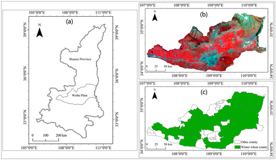
Figure 1.
Overview of the study region: (a) location of the Weihe Plain; (b) FY-3D false colour composite image for 3 May 2020; and (c) locations of the county-scale WWY data points used in the WWY estimation.
2.2. RS Data and Y Data
The RS data used in this study included 20 m SR Sentinel-2 MSI surface reflectance data, 250 m SR FY-3D MERSI surface reflectance data from early March to late May in 2020 to 2022, and 500 m SR Aqua MODIS GPP product (MYD17A2H) data at 8 day intervals from March to May 2014–2022. Among them, the Sentinel-2 data were obtained from the Sentinel Scientific Data Hub, the FY-3D data were obtained from the FY Satellite RS Data Service Network, and the MYD17A2H product was obtained from the Atmospheric Storage and Distribution System (LAADS) Distributed Active Storage Center (DAAC). According to the main WW growing period on the Weihe Plain, only the data from early March to late May were used for the STDF and WWY estimation. Table 1 lists the acquisition dates (AQDs) of the Sentinel-2 and FY-3D data, which were acquired under cloudless conditions. Since more Sentinel-2 data were available in 2020 and were evenly distributed between early March and late May, the EDCSTFN was trained on the 2020 data, and the trained model was subsequently applied to the 2021 and 2022 data. To obtain the geometrically corrected reflectance products, the Sentinel-2 data were processed using the Sentinel Application Platform (SNAP) 9.0, the FY-3D data were processed by using the SMART 3.2 software that can be downloaded from the FY Satellite RS Data Service Network and the MODIS data were processed by using the MODIS Reprojection Tool (MRT). After analyzing the Sentinel-2 and FY-3D imagery, the Sentinel-2 imagery exhibited high geometric correction precision, and no further mutual registration was needed. Moreover, the FY-3D imagery exhibited relatively low geometric correction precision, and geometric bias occurred between the images for different dates. Therefore, the obtained FY-3D images were further registered with the Sentinel-2 imagery. First, the cloudless Sentinel-2 surface reflectance imagery was selected as the reference imagery and resampled to the SR of the FY-3D imagery (approximately 250 m). Then, the ENVI 5.3 software was used to automatically register the FY-3D surface reflectance imagery with the Sentinel-2 imagery. To ensure stable registration, the first-order polynomial was selected for automatic registration. Based on the registered Sentinel-2 and FY-3D surface reflectance data, the NDVI, SAVI and EVI were calculated, and then, maximum value composites were generated to obtain the 10 day interval FY-3D VI. For any 10 day intervals lacking available FY-3D data (e.g., mid-May 2021), the average VI imagery of the first and next 10 day periods were used as the FY-3D VI imagery for these 10 day intervals. Since there was only one Sentinel-2 image for each 10 day interval during the study period, the Sentinel-2 VI imagery was directly used as the 10 day period VI imagery. In this study, the calculated 10 day period FY-3D and Sentinel-2 VI images were used for the STDF, and the obtained MYD17A2H products were used for WWY estimation. In the process of STDF, the FY-3D images were reprojected and resampled to the projection and SR (20 m) of the Sentinel-2 data.

Table 1.
AQDs of the Sentinel-2 and FY-3D data under cloudless conditions.
In addition, to construct and evaluate the precision of the WWY estimation model for the Weihe Plain, the WWY statistical yearbook data from 2020 to 2021 from 24 counties on the Weihe Plain (Figure 1c) covering numerous WW planting areas, most of which are located in the study region, were selected. The statistical yearbook data related to the counties on the Weihe Plain for 2022 were temporarily unavailable. Therefore, the WWY estimation results for 2022 were not verified in this study.
2.3. Methods
The method framework in this study involved two steps (Figure 2): spatiotemporal fusion of the 10 day interval VIs based on Sentinel-2 and FY-3D data and farmland-scale WWY estimation. (1) In the process of spatiotemporal fusion of the VIs, the ESTARFM and EDCSTFN were used to fuse the 10 day interval NDVI, SAVI and EVI images from Sentinel-2 and FY-3D, respectively, thereby reconstructing the 10 day interval VI imagery with a 20 m SR over the WW growing period. The fusion precisions of the two models were compared in this study. (2) In the process of farmland-scale WWY estimation, a BPNN WWY estimation model was constructed to estimate the WWY on the Weihe Plain with a 20 m SR based on spatiotemporally fused VI imagery, and the Aqua MODIS GPP product (MYD17A2H) and the county-scale WWY statistical data were used to construct the WWY estimation model. The key methods are described in this section.
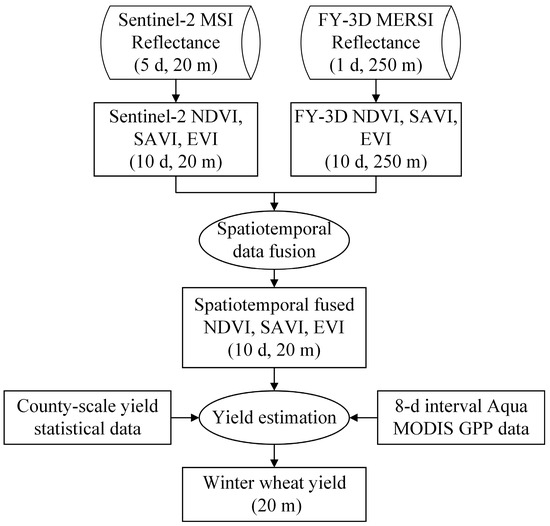
Figure 2.
Flowchart of the 10 day interval VI imagery reconstruction and farmland-scale WWY estimation.
2.3.1. Spatiotemporal Fusion of VIs Based on Sentinel-2 and FY-3D Data
In accordance with the principles and uses of the ESTARFM and EDCSTFN described by Zhu et al. [34] and Tan et al. [37], in this section, the training scheme of the EDCSTFN and the usage and parameter setting scheme of the two models for spatiotemporal fusion of the 10 day interval Sentinel-2 and FY-3D VI imagery are described.
The EDCSTFN is a spatiotemporal fusion model based on convolutional neural network autoencoders with an encoder-feature fusion-decoder architecture. The model consists of two encoders: an encoder for FSR imagery and a residual encoder. The encoder for FSR imagery learns the features of the FSR reference imagery, and the residual encoder learns the feature changes in the FSR reference imagery between the reference and predicted imagery dates based on the input FSR and CSR imagery. The fusion process is performed in the feature space. The feature imagery of the FSR reference imagery is added to the feature imagery output by the residual encoder, and the resulting decoder is subsequently used to restore the fused feature imagery to the original pixel space. To evaluate the feature loss of the fusion results, an hourglass-shaped autoencoder is also built into the EDCSTFN to extract features from both the fusion and validation images. In the date-setting scheme of this study, Sentinel-2 NDVI, SAVI, and EVI images from 28 April 2020, were used to train the autoencoders to evaluate the feature loss of each VI. The main parameters of the EDCSTFN include the initial learning rate of the Adam optimization algorithm, the number of training epochs, the batch size, the size of the training images, and the size of the prediction images. In this study, the initial learning rate was set to 0.001. In addition, the number of training epochs was set to 100, and the training process was stopped when the learning rate decreased to 1 × 10⁻⁵. The training batch size was set to 4 according to our hardware configuration. In addition, the structures of the encoders and decoders in the EDCSTFN and the settings of the hyperparameters and the regularization method of the Adam optimization algorithm are the same as those in the method discussed in Tan et al. [37].
During the EDCSTFN training stage, according to the method described in Zhou et al. [42], two areas of 1500 × 1500 pixels were selected from the cropland areas in the western and central parts of the Weihe Plain, two of which were randomly selected as training images and the other two as validation images. When the data AQD were selected for EDCSTFN training, the AQDs of the Sentinel-2 and FY-3D VI images for early March, early April, late April and mid-May 2020 were combined as reference and predicted imagery dates. In each training area, six sets of data were selected for EDCSTFN training during the main WW growing period on the Weihe Plain (Table 2). The EDCSTFN requires 1–2 pairs of FSR imagery and CSR imagery acquired on similar dates as the reference imagery. During the training process implemented in this study, only one pair of reference images was used, and the EDCSTFN trained on the 2020 data were used to predict the 10 day interval VI imagery during the main WW growing period at the farmland scale in 2021 and 2022.
Table 2.
Data AQD for EDCSTFN training in 2020.
At the EDCSTFN prediction stage, the size of the prediction imagery was set to 7980, and the full imagery of the Weihe Plain was divided into two parts, each containing 7980 × 7980 pixels. To reconstruct the farmland-scale 10 day interval VI imagery during the main WW growing period, evaluate the impact of the STDF period length (i.e., the distance between the AQD of the two reference images) on the prediction precision, and considering the availability of Sentinel-2 data at each WW growing stage on the Weihe Plain from 2020 to 2022, the Sentinel-2 and FY-3D VI images obtained during different 10 day periods were selected as the reference imagery for the fusion model. The specific fusion scheme for each year is as follows: (1) In 2020, the VI imagery obtained in early March and late April and the VI imagery obtained in early April and mid-May were selected as reference imagery for the fusion model (with an interval of approximately 1.5 months) to predict the farmland-scale 10 day interval VI imagery between the AQDs of the two reference images. The prediction results were compared with those when the VI imagery acquired in early March and mid-May was selected as the reference imagery (with an interval of approximately 2.5 months). (2) In 2021, the VI imagery obtained in late March was selected as the reference imagery for predicting the farmland-scale VI imagery for early and mid-March. (3) In 2022, the VI imagery obtained in early and late April was selected as the reference imagery for predicting the farmland-scale VI imagery for early and mid-April, and the VI imagery obtained in early May was selected as reference imagery to predict farmland-scale VI imagery for mid- and late May. (4) In 2022, the VI imagery obtained in early and late April as well as the VI imagery obtained in late April and late May were selected as the reference imagery (with an interval of approximately 1.5 months) to predict the farmland-scale 10 day interval VI imagery between the AQDs of the two reference images. In addition, the prediction results were compared with those when the VI imagery acquired in early March and late May was selected as the reference imagery (with an interval of approximately 2.5 months).
The ESTARFM requires two FSR images as reference images. Thus, the fusion schemes of the ESTARFM from early March to mid-May 2020, from late March to late April 2021, and from early March to late May 2022 were the same as those of the EDCSTFN. In the ESTARFM parameter settings, according to the method from Zhou et al. [41], the number of categories was set to 10 according to the land cover in the study region. In addition, the moving window size was set to 25 Sentinel-2 VI pixels, corresponding to approximately two FY-3D VI pixels.
2.3.2. WWY Estimation Based on the Spatiotemporally Fused VIs
The WWY estimation framework comprises two parts: WWY estimation based on the MODIS cumulative GPP data (Figure 3a) and farmland-scale WWY estimation based on multiple parameters (Figure 3b). First, a linear regression WWY estimation model based on the MODIS cumulative GPP and county-scale WWY data were constructed to generate WWY data for the Weihe Plain with an SR of 500 m, and a BPNN WWY estimation model based on the spatiotemporally fused NDVI, SAVI and EVI data from across multiple growing stages was then constructed. The WWY data with an SR of 500 m were used to train the BPNN WWY estimation model, thereby estimating the farmland-scale WWY on the Weihe Plain. The two parts of the method are described in detail in this section.

Figure 3.
Flowchart of farmland-scale WWY estimation: (a) Y estimation model based on the cumulative GPP; and (b) farmland-scale Y estimation model based on multiple parameters.
In the process of constructing a WWY estimation model based on the cumulative GPP, the MODIS GPP data for the Weihe Plain from March to May were first collected to obtain the cumulative GPP data for the main WW growing period. According to the distribution of the WW planting areas on the Weihe Plain reported by Zhou et al. [45] and the county boundaries of the Weihe Plain, the 500 m SR cumulative GPP data for the overall WW planting area were averaged to the county scale, thereby obtaining the average cumulative GPP of WW for the main growing period of each county on the Weihe Plain. Many studies have shown that WWY data exhibit a favourable linear relationship with the cumulative GPP during the growing period [53,54]. In this study, a linear regression model was established between the average cumulative GPP and WWY statistics for each county on the Weihe Plain from 2014 to 2018. This model was used to estimate WWY data with a 500 m SR for 2020 to 2022. Due to the increase in cloud cover over the Weihe Plain from March to May 2019, the GPP data for 2019 were not used for WWY estimation. The R2 value and the p-value of the hypothesis test were used to assess the correlation between the MODIS cumulative GPP data and WWY statistical data.
In the process of farmland-scale WWY estimation based on multiple parameters, the 10 day interval VI (including the NDVI, SAVI and EVI) images at the farmland scale reconstructed by the STDF model were averaged to obtain farmland-scale VI imagery for the 4 WW growing stages. Then, farmland-scale VI images for the 4 WW growing stages were used as input data, and the WWY data estimated from the MODIS cumulative GPP data were used as the target sample to construct a BPNN Y estimation model based on spatiotemporally fused VI imagery. In the BPNN Y estimation model, a single hidden layer neural network containing 5 neurons was used. The number of neurons in each layer of the model and the activation function are provided in Table 3. The specific steps used to construct a WWY estimation model based on the BPNN were as follows: (1) the farmland-scale VI images for the 4 WW growing stages were aggregated to a 500 m SR; (2) a BPNN Y estimation model based on the spatiotemporally fused VI imagery for the 4 growing stages and the WWY data estimated from the MODIS cumulative GPP data were constructed and trained at a 500 m SR, where the training and validation data accounted for 90% and 10% of the total data, respectively; (3) the farmland-scale VI imagery for each WW growing stage was entered into the BPNN Y estimation model, thereby estimating the WWY at the farmland scale; and (4) the WWY estimation results of the BPNN were evaluated by using the county-scale WWY statistical data for the Weihe Plain.
Table 3.
Structure and parameters of the BPNN WWY estimation model.
2.3.3. Precision Evaluation of the STDF and WWY Estimation Model
The consistency of the FSR imagery and CSR imagery may affect the precision of the spatiotemporal fusion results [39]; therefore, it is necessary to verify the consistency of the 10 day interval VI imagery between Sentinel-2 and FY-3D before spatiotemporal fusion. To test the consistency of the 10 day interval Sentinel-2 and FY-3D VI (including NDVI, SAVI and EVI) imagery, the Sentinel-2 VI imagery during the study period was aggregated to 250 m and compared with the FY-3D VI imagery for the same 10 day period.
In the precision evaluation of the STDF model, the data from 2020 to 2022 were used to evaluate the impact of different reference date distances (at intervals of approximately 1.5 and 2.5 months) on the prediction precision of the ESTARFM and EDCSTFN. The fusion results were evaluated by using Sentinel-2 VI imagery that was not used in the STDF process. Due to the lack of data for the corresponding period in 2021, the data for 2021 were not used in the above test but were only used to reconstruct 10 day interval VI imagery at the farmland scale.
To evaluate the precision of the WWY estimation, the WWY statistical yearbook data from 2020 to 2021 for 24 counties on the Weihe Plain were used to evaluate the precision of the BPNN WWY model based on the spatiotemporally fused VI imagery. The WWY estimate results were averaged to the scales of each county, and the linear regression method was employed to correlate the WWY estimate results with the WWY statistical yearbook data at the county scale.
To quantify these precision evaluations, the coefficient of determination (R2), root mean square error (RMSE), and average deviation (predicted results—validation data) were used to evaluate the precision of the STDF results and the WWY estimation results. These metrics are important indices for evaluating the differences between model estimation results and validation data. In this work, the random and systematic deviations between the fusion results and validation imagery, as well as the random and systematic deviations between the WWY estimation results and validation data, were evaluated by these indices.
3. Results
3.1. Consistency of the VIs Between Sentinel-2 and FY-3D
The consistency of the 10 day interval Sentinel-2 and FY-3D VI (including the NDVI, SAVI and EVI) imagery was tested by using the method described in Section 2.3.2. The consistency validation results for early March, early April, late April, and mid-May 2020 are displayed in Figure 4. The R2 values between the aggregated Sentinel-2 VI imagery and the FY-3D VI imagery varied between 0.22 and 0.35, and the RMSE values of the fitting results varied between 0.09 and 0.14. The R2 values of the NDVI, SAVI and EVI imagery were essentially consistent. These results also revealed large random deviations between the 10 day interval FY-3D VI imagery and the aggregated Sentinel-2 VI imagery, and the random deviations corresponding to the NDVI, SAVI and EVI imagery were basically the same. These random deviations may be related to differences in the satellite overpass time, satellite observation angle, spectral response characteristics of the bands, atmospheric correction and registration precision between Sentinel-2 and FY-3D [39], especially the registration precision of the FY-3D imagery. In this study, the FY-3D imagery still exhibited deviations of 1–2 pixels between the different dates after 1-degree polynomial registration. In addition, the average deviations between the FY-3D VI imagery and aggregated Sentinel-2 VI imagery varied mostly between −0.02 and 0.02, which indicates that the systematic deviations of the 10 day interval VI imagery between Sentinel-2 and FY-3D are small. Therefore, the STDF model could be used to fuse the 10 day interval VI imagery of Sentinel-2 and FY-3D. However, due to the large random deviations of the 10 day interval VI imagery between Sentinel-2 and FY-3D, it is necessary to select an STDF model that is insensitive to random deviations. The ESTARFM employs a sliding window to search for similar pixels and applies a weighted function to reduce the effect of random errors, and the EDCSTFN is an STDF model based on convolutional neural networks in which random errors can be reduced through the convolution operation. Therefore, both the ESTARFM and EDCSTFN can reduce the random deviations of the fusion data. The precision of the ESTARFM and EDCSTFN for the spatiotemporal fusion of the 10 day interval Sentinel-2 and FY-3D VI imagery is evaluated below.
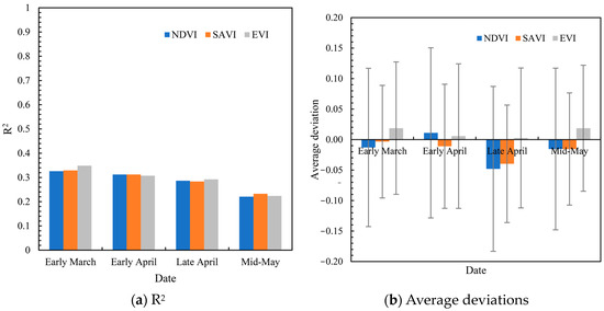
Figure 4.
Results of the consistency analysis of the Sentinel-2 and FY-3D VIs: (a) R2 values between the aggregated Sentinel-2 VI imagery and the FY-3D VI imagery at an SR of 250 m; and (b) average deviations and RMSE values of the fitting results between the aggregated Sentinel-2 VI imagery and FY-3D VI imagery. The error line in (b) denotes the RMSE of the fitting results.
3.2. VI Spatiotemporal Fusion Results
3.2.1. Training of the EDCSTFN
The established EDCSTFN based on the Sentinel-2 and FY-3D VIs (including the NDVI, SAVI and EVI) was trained according to the training data grouping scheme discussed in Section 2.3.1. After approximately 50 training iterations, the model gradually converged; the loss for the model converged at approximately 0.03, and the value of the training loss was very close to that of the validation loss. Table 4 displays the values of the final training and validation losses for training the EDCSTFN with different data grouping schemes. Among them, the values of the training and validation losses obtained by using the training datasets for early April and late April were the smallest among all of the groups, varying between 0.020 and 0.031, followed by the training datasets for early March and early April, with values varying between 0.024 and 0.030. The values of the training and validation losses corresponding to the training datasets for late April and mid-May were the largest, varying between 0.029 and 0.044, and the values of the training and validation losses obtained using all of the datasets for March to May were centred at all the groups, varying between 0.028 and 0.042. The above results are similar to the results based on the Sentinel-2 and Sentinel-3 images published by Zhou et al. [42]. These results indicate that the EDCSTFN provides greater precision for spatiotemporal fusion of the 10 day interval Sentinel-2 and FY-3D VI imagery for April, followed by March, with a lower spatiotemporal fusion precision for May. The model trained by using all of the datasets for March to May achieved high overall precision over the main WW growing period. Therefore, in practical applications, to increase the convenience of the EDCSTFN, the model trained by using all of the datasets for the period from March to May was uniformly employed to predict the 10 day interval VI imagery at the farmland scale during the main WW growing period.
Table 4.
Training and validation losses for EDCSTFN training.
3.2.2. Prediction by the EDCSTFN
The precisions of the EDCSTFN and ESTARFM were evaluated according to the date selection scheme employed during the prediction stage of the spatiotemporal fusion models described in Section 2.3.1, and farmland-scale 10 day interval VIs (including the NDVI, SAVI and EVI) were predicted during the main WW growing periods from 2020 to 2022. To assess the spatiotemporal fusion precision of the EDCSTFN and ESTARFM, at a distance of approximately 1.5 months between the AQDs of the two reference images, the Sentinel-2 and FY-3D VI images acquired in early March and late April 2020, early April and mid-May 2020, early March and late April 2022, and late April and late May 2022 were used as reference images to predict farmland-scale 10 day interval VI images between the AQDs of the reference images (including early April, late April and early May). The R2 values and average deviations between the spatiotemporal fusion results and Sentinel-2 VI imagery used for validation are listed in Table 5. In 2020, the R2 value between the predicted results of the EDCSTFN and ESTARFM and the Sentinel-2 VI data were approximately 0.9, and the absolute value of the average deviation in most 10 day periods did not exceed 0.03. These results are similar to the precision of the fusion results based on other satellite sensors (such as MODIS and Landsat) in previous studies [45,55,56,57], which indicates that both the EDCSTFN and ESTARFM can obtain high precisions when fusing FY-3D and Sentinel-2 VI imagery of the Weihe Plain when the distance between the acquisition and reference imagery dates is approximately 1.5 months. In addition, the R2 values and average deviations corresponding to the predicted results of the EDCSTFN in 2022 are basically the same as those of the ESTARFM and are very close to the prediction precision of the EDCSTFN in 2020, which indicates that the EDCSTFN trained on single-year data still achieves satisfactory spatiotemporal fusion precision in the adjacent years.
Table 5.
Fusion precision evaluation of the EDCSTFN and ESTARFM when the distance between the reference imagery AQD is approximately 1.5 months. RMSEfit represents the RMSE of the fitting results, and AD represents the average deviation.
To further analyze the spatiotemporal fusion precision of the EDCSTFN and ESTARFM when the distance between the AQDs of the two reference images is approximately 2.5 months, Sentinel-2 and FY-3D VI imagery acquired in early March and mid-May 2020 were used as reference imagery to predict the farmland-scale VI imagery for early and late April 2020, and Sentinel-2 and FY-3D VI imagery acquired in early March and late May 2022 were used as reference images to predict the farmland-scale VI imagery for early April and early May 2022. The R2 values and average deviations of the spatiotemporal fusion results are listed in Table 6. Compared with the fusion precisions when the distance between the reference imagery AQD is approximately 1.5 months, the precisions of both the EDCSTFN and ESTARFM significantly decrease for a period of approximately 2.5 months between the reference imagery AQD. The R2 values of the EDCSTFN are above 0.75, and the R2 values of the ESTARFM are above 0.68. These results indicate that the performance of both the EDCSTFN and ESTARFM decreases when the spatiotemporal fusion period of the VIs increases. However, the deep learning-based EDCSTFN could obtain a higher prediction precision. Considering the influence of the distance between the reference imagery AQD and the precision of the spatiotemporal fusion models, the distance between the reference imagery AQD was ultimately maintained at approximately 1.5 months, and the EDCSTFN was employed to reconstruct the farmland-scale 10 day interval VI imagery for the main WW growing period on the Weihe Plain for the 2020–2022 period, thereby achieving WWY estimation at the farmland scale.
Table 6.
Fusion precision evaluation of the EDCSTFN and ESTARFM when the distance between the reference imagery AQD is approximately 2.5 months. RMSEfit represents the RMSE of the fitting results, and AD represents the average deviation.
3.2.3. Farmland-Scale EVI Images of WW During Each Growing Period
Notably, 20 m SR NDVI, SAVI and EVI imagery for the 4 WW growing stages were obtained by averaging the 10 day spatiotemporally fused NDVI, SAVI and EVI imagery for the main WW growing periods from 2020 to 2022. Under the influence of clouds, only one cloudless Sentinel-2 image of the Weihe Plain could be obtained for each WW growing period, and a single image cannot reflect the average crop growth during each growing stage. However, the average treatment of the reconstructed 10 day scale VI imagery for each WW growing stage could better reflect the average crop growth during each growing stage. Figure 5 shows the 20 m SR EVI imagery for the 4 growing stages on the Weihe Plain from 2020 to 2022, which was reconstructed by using the EDCSTFN. Between March and May of each year, the areas with notable changes in EVI values were mainly WW planting areas, and the changes in EVI values in forest areas were relatively small. Among the 4 WW growing stages, the EVI values in the WW planting area were usually the highest at the heading-filling stage, followed by those at the jointing and milk stages, and the EVI values at the regrowth stage were usually the lowest, as was the case for the EVI on the Weihe Plain in 2021 and 2022. However, the maximum EVI values in the WW planting areas in 2020 occurred earlier than those in 2021 and 2022, namely, from late March to mid-April, corresponding to the jointing stage in 2021 and 2022. In the WW planting area on the western Weihe Plain, the EVI values before late March were greater than those from late April to early May in 2020. These results indicate that the actual heading-filling stage of the WW on the western Weihe Plain in 2020 occurred earlier than that in 2021 and 2022, which could be related to the early WW sowing time in 2020. In addition, when comparing the EVI values in the WW planting areas in the different regions of the Weihe Plain from 2020 to 2022, the EVI values of the WW planting areas in the western Weihe Plain were greater than those in the central part of the Weihe Plain during the first three growing stages. Previous studies have indicated that the growth characteristics of WW on the Weihe Plain from late March to late April (including the jointing and heading-filling stages) are important for Y estimation [58]. The growth in the WW planting area in the western Weihe Plain was greater than that in the central part of the Weihe Plain, and the Y in the western Weihe Plain was also greater.
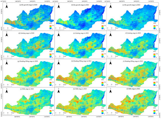
Figure 5.
EVI at each WW growing stage from 2020 to 2022.
3.3. Farmland-Scale WWY Estimation Results and Analysis
3.3.1. WWY Estimation Results Based on the Cumulative GPP
According to the method description of WWY estimation based on the MODIS cumulative GPP data in Section 2.3.2, eight day-scale Aqua MODIS GPP data for the main WW growing period (from March to May of each year) from 2014 to 2018 were collected, and a linear regression model relating the cumulative GPP data for the main WW growing period over the five-year period and the county-scale WWY statistical data were constructed in this study (Figure 6a). The regression results reveal that the cumulative GPP data for the main WW growing period on the Weihe Plain from 2014 to 2018 were strongly correlated with the WWY statistical data at the county scale, with an R2 value of 0.67 (p < 0.01). These results indicate that the WWY on the Weihe Plain with a 500 m SR could be accurately estimated based on the cumulative MODIS GPP data for multiple years. Therefore, the linear regression model for WWY estimation based on the MODIS cumulative GPP data were then used to estimate the WWY at a 500 m SR on the Weihe Plain from 2020 to 2022 (Figure 7). The high-Y areas of WW on the Weihe Plain were distributed mainly in the western and central parts, and the WWY in the western Weihe Plain was slightly higher than that in the central part of the Weihe Plain. These findings are similar to the analysis results of the spatial distribution of Y based on the EVI discussed in Section 3.2.3. Compared with that in 2020, the Y in the main WW planting areas of the Weihe Plain slightly increased in 2021, while the Y decreased in 2022 to values lower than those in 2020 and 2021. The estimation results of the WWY based on the MODIS cumulative GPP data were also verified using the WWY statistical data for the counties on the Weihe Plain from 2020 to 2021. The results reveal that the WWY estimation results were linearly correlated with the WWY statistical data at the county scale, with R2 values reaching 0.65 and 0.63, respectively (p < 0.01) (Figure 6b and 6c, respectively). Therefore, the WWY estimation results at a 500 m SR could be used to train a farmland-scale WWY estimation model with multiple parameters.
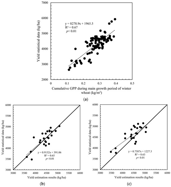
Figure 6.
Y estimation model based on the cumulative GPP for the main WW growing period and the Y estimation precision evaluation results in 2020 and 2021. The dotted lines in the figures denote the fitted linear functions, which are close to the diagonal solid lines, indicating that the systematic deviation in the Y estimation results is small. (a) Linear regression model between the cumulative GPP data for the main WW growing period and the county-scale WWY from 2014 to 2018, (b) linear regression results between the WWY estimation results from 2020 based on the cumulative GPP and county-scale Y statistical data, and (c) linear regression results between the WWY estimation results in 2021 based on the cumulative GPP and county-scale Y statistical data.
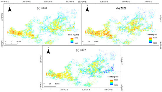
Figure 7.
WWY estimation results for 2020 to 2022 based on the MODIS cumulative GPP data.
3.3.2. Training Results of the Farmland-Scale WWY Estimation Model Based on Multiple Parameters
The NDVI, SAVI and EVI imagery for the four WW growing stages from 2020 to 2022 were aggregated to the 500 m SR, and a BPNN model was constructed between the multiple VIs (including the NDVI, SAVI and EVI) at the four growing stages and the WWY at the 500 m SR. Table 7 lists the training and validation precisions of the BPNN WWY estimation model from 2020 to 2022. The R2 values corresponding to the training and validation precisions of the BPNN model reached 0.67 (p < 0.01), indicating a satisfactory fitting ability. The BPNN Y estimation model constructed by integrating the VIs at the four WW growing stages could provide highly accurate WWY estimates. Compared with that in 2020, the training precision in 2021 and 2022 decreased, which could be related to the Y estimation errors based on the MODIS GPP data. The R2 value between the Y estimates based on the cumulative GPP and county-scale WW statistical data in 2021 was slightly lower than that in 2020, and the systematic deviation was larger than that in 2020 (Figure 6). Over time, crop varieties and technologies will continue to improve [59], which will lead to increasing uncertainty in WWY estimation models based on GPP data from 2014 to 2018. Therefore, to obtain a higher Y estimation precision, a Y estimation model based on cumulative GPP data should be retrained using the latest yearly data in the future.
Table 7.
Training and validation precisions of the multiparameter WWY estimation model based on the BPNN.
3.3.3. Results and Analysis of WWY Estimation at the Farmland Scale
The farmland-scale spatiotemporally fused NDVI, SAVI and EVI imagery for the four WW growing stages from 2020 to 2022 were input into the BPNN WWY estimation model, which was used to estimate the farmland-scale WWY on the Weihe Plain from 2020 to 2022. Figure 8 shows the farmland-scale Y estimation results of the BPNN model based on the NDVI, SAVI and EVI from 2020 to 2022. The spatial distribution of the WWY estimation results and the variation pattern over 3 years were basically consistent with the 500 m SR results estimated based on the MODIS cumulative GPP data (Figure 7). The WWYs in the main planting areas varied mainly between 4000 and 6000 kg/ha, with the highest Y occurring in 2021, followed by 2020, and the lowest Y occurring in 2022. On the Weihe Plain, the WW planting area in Baoji City attained the highest Y, followed by the central part of the Weihe Plain, which is located at the junction of Xi’an City and Weinan City. The distribution of the WW planting areas in the other areas of the Weihe Plain was relatively sparse, and the Y was relatively low. These results are consistent with the corresponding annual statistical yearbook data. The R2 values between the WWY statistical data at the county scale and the Y estimation results based on the BPNN model in 2020 and 2021 reached 0.78 and 0.68, respectively (Figure 9), revealing a favourable correlation between the Y estimation results and the Y statistical data at the county scale. These results indicate that the BPNN model, which is based on spatiotemporally fused VIs across multiple WW growing stages, provided suitable Y estimation precision for WW on the Weihe Plain, and the results were better than the Y estimation results based on the MODIS cumulative GPP data (with R2 values of 0.65 and 0.63 in 2020 and 2021, respectively). In addition, the WWY estimation results at an SR of 20 m clearly reveal the difference in WWY between adjacent farmlands, indicating that the WWY estimation results based on the spatiotemporally fused VIs better reflect the detailed characteristics of the farmland-scale WWY distribution on the Weihe Plain.
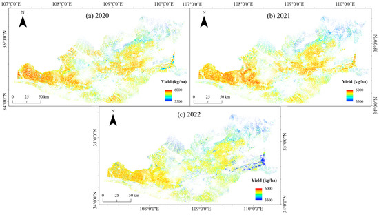
Figure 8.
Farmland-scale WWY estimation results for the Weihe Plain from 2020 to 2022 based on multiple parameters.
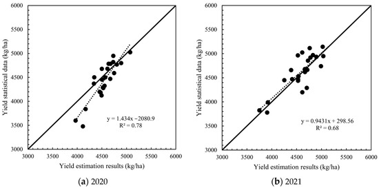
Figure 9.
Linear regression results between the farmland-scale WWY estimation results and the Y statistical data in 2020 and 2021. The dotted lines in the figures denote the fitted linear functions, which are close to the diagonal solid lines, indicating that the systematic deviation of the Y estimation results is small.
4. Discussion
To address the problem of limited research based on the Chinese meteorological satellite FY-3 series (such as FY-3D) in the fields of STDF and farmland-scale WWY estimation, a method framework for 10 day interval VI (NDVI, SAVI and EVI) reconstruction based on the FY-3D MERSI and Sentinel-2 MSI data and farmland-scale WWY estimation based on reconstructed VI imagery was proposed in this paper. The ability of the deep-learning-based EDCSTFN to perform spatiotemporal fusion of 10 day interval VI imagery of the Weihe Plain based on FY-3D MERSI and Sentinel-2 MSI data were assessed in this study by compared with ESTARFM. The results in Section 3 showed that both the EDCSTFN and ESTARFM achieved satisfactory spatiotemporal fusion precision and could effectively provide farmland-scale WWY estimation. The precision evaluation results in this study are similar to the precision of the fusion results based on other satellite sensors (such as MODIS and Landsat) as well as the other study regions in previous studies [45,55,56,57]. In addition, when the date range of the STDF is long, the deep learning-based EDCSTFN achieves higher precision. Therefore, this study is meaningful for accurate farmland-scale growth monitoring and Y estimation of WW based on Chinese FY-3 meteorological satellite data. However, the STDF based on the FY-3D MERSI VIs and farmland-scale WWY estimations should still be investigated. The research prospects of these two components are described in this section.
4.1. Research Prospects of the STDF
4.1.1. Computational Efficiency
The computational efficiency of the STDF model is one of the important factors affecting its application prospects. The traditional weight function-based spatiotemporal fusion model spends much of its time searching for similar pixels by using sliding windows [31]. Approximately 3 h is needed to use the ESTARFM to fuse the Sentinel-2 and FY-3D imagery of the Weihe Plain once (an Intel Core i7-12700h CPU and 2.30 GHz were used in the test). Thus, it is difficult to apply this model in the WW planting areas of the whole country. The deep learning-based spatiotemporal fusion model does not use a sliding window to find similar pixels. After testing, the computational time required by the EDCSTFN at the prediction stage was much shorter than that of the ESTARFM. The EDCSTFN only needed approximately 10 min to fuse the Sentinel-2 and FY-3D images of the Weihe Plain with the same equipment configuration. In addition, the EDCSTFN trained on single-year data could still be used for near-future analysis, and the fusion precision remained basically unchanged. Therefore, the trained EDCSTFN exhibits greater application potential in the STDF of large areas and long time series. In the future, we will further research the method of transferring the EDCSTFN trained on the WW planting area on the Weihe Plain to other WW planting areas in China and assess its spatiotemporal fusion precision.
4.1.2. TR of FSR and CSR Imagery
To obtain high spatiotemporal fusion precision, it is usually necessary to acquire at least one Sentinel-2 image for each WW growing stage, especially the heading-filling and milk stages, when WW grows rapidly. However, due to the effects of clouds, the TR (5 days) of the Sentinel-2 satellite images can sometimes barely meet the above requirements. At present, the Chinese GF series satellites have undergone long-term development. The GF-6 satellites, which were launched in June 2018, can obtain multispectral imagery with an SR of 16 m, exhibiting high band consistency with the GF-1 satellite launched in 2013. With the networking of the GF-1 and GF-6 satellites, 16 m SR multispectral imagery with a TR of 2 days can be obtained [60]. In addition, since the swath widths of GF-1 and GF-6 reach 800 km, they are more suitable when employing the STDF in large areas. In the future, a spatiotemporal fusion method based on GF series data and FY-3 data will be developed.
On the other hand, the TRs of the CSR imagery are also important for time series’ reconstructions of VI imagery at the farmland scale. Considering the effects of clouds, a 10 day interval VI reconstruction method at the farmland scale based on the FY-3D and Sentinel-2 satellite data were proposed in this paper. With the successful launch of the FY-3F satellite in August 2013 and the replacement of the FY-3C satellite, which has been operating for nearly 10 years, the monitoring capability of the FY-3 polar-orbiting meteorological satellites in the morning will continue to increase. In the future, a time series VI reconstruction method at the farmland scale based on the FY-3D/F and Sentinel-2 satellites will be developed, which will improve the TR of time series farmland-scale VI reconstructions (from 10 day intervals to 5 day intervals).
4.1.3. Registration Precision of the Imagery in the STDF
The registration precision of the RS imagery may notably influence the precision of the STDF model [31]. The results in Section 3 show that the STDF based on the Sentinel-2 and FY-3D data in this study yields high precision since the geometric correction precision of Sentinel-2 imagery is high, although there is a large random deviation between the Sentinel-2 and FY-3D VI imagery due to factors such as geometric correction errors in the FY-3D imagery. However, regarding the Chinese FSR satellites such as GF-1, due to the use of instruments and algorithms, the current mutual geometric correction precision cannot reach the level of Sentinel-2 [61]. Therefore, the STDF for the GF-1 satellites may involve high uncertainties. In the future, the fusion precision of Chinese FSR satellites and FY-3 satellites will be further analyzed, and a fusion model with low sensitivity to registration precision will be developed.
4.1.4. Difference in the SR Between the FSR and CSR Imagery
The difference in the SRs between the FSR and CSR imagery significantly affects the precision of the spatiotemporal data fusion models. Compared with FSR imagery, there are fewer spatial details of the ground features in CSR imagery, especially in regions with abrupt changes in land cover, such as regions with newly harvested WW and areas affected by floods [31]. To address the conversion relationship between the land surface features in FSR and CSR imagery at different scales, the ESTARFM and EDCSTFN build linear models and deep convolutional neural network models, respectively, to fit and learn the conversion relationship of the land surface features between the FSR and CSR imagery [34,37]. However, there are still uncertainties in areas with irregular abrupt changes in land cover type. Therefore, the reliability of the STDF has a negative correlation with the differences in the SRs between FSR and CSR imagery. Compared with the STDF, super-resolution technology can improve the SR of remote sensing imagery with fewer requirements, such as a sufficient amount of reference imagery [62]. Although the precision of super-resolution models may be lower than that of STDF models in terms of the reference imagery when the difference in the SR between the input image and target image is large, the super-resolution models can be used to appropriately improve the SR of CSR images, thereby providing a novel way to improve the precision of STDF models. In recent years, researchers have developed many super-resolution models, such as super-resolution generative adversarial networks (SRGANs) [63], enhanced SRGANs (ESRGANs) [64], the real-ESRGAN [65], and the improved SRGAN (ISRGAN) [62], which have been successfully applied to the spatial downscaling of satellite imagery, such as MODIS [62,66]. In the future, a super-resolution model will be introduced to the current FY-3D-based farmland-scale WWY estimation method framework, and improvements in the precision of the STDF model and WWY estimation model will be tested further.
4.2. Research Prospects of the WWY Estimation Model
There is a complex nonlinear relationship between the WWY and the various VIs, including the NDVI, SAVI, and EVI. Therefore, the construction of a WWY estimation model requires a large amount of training data. However, the amount of WWY data currently available cannot satisfy the training requirements of complex WWY estimation models. In addition, meteorological and soil factors such as temperature, precipitation and soil moisture also greatly impact the WWY [67]. Therefore, the impacts of meteorological and soil factors must be considered in multiyear WWY estimation. The WW time series GPP data consider the influence of meteorological factors on the growth of WW, and there was a high correlation between the cumulative GPP data for the main growing period and the WWY [53,54]. Therefore, the MODIS cumulative GPP and multiyear WWY data at the county scale were used to establish a linear regression model in this study. The model was subsequently used to estimate the multiyear WWY with an SR of 500 m and then employed to train the annual WWY estimation model based on the BPNN. The above method framework is often sub-optimal for WWY estimation compared to the WWY estimation model based directly on VI imagery and meteorological parameters. In the future, many ground-based measuring plots for the WWY will be constructed in the WW planting regions in China, which will provide support for the construction of complex machine learning models based on many feature parameters. In addition, sensitivity analyses will be performed to explore the impact of different parameters on the WWY, thereby selecting the effective parameters to construct the WWY estimation model.
In addition, continuous time series VI data provide a large amount of information related to the WWY on different dates during the growing period. Thus, traditional machine learning models may not fully utilize the effective information contained in continuous time series data and may even lead to overfitting. To reduce overfitting, the VI data from 10 day intervals were aggregated into 4 WW growing stages in this work, thereby greatly reducing the number of input parameters for the Y estimation model. However, much of the effective information related to the WWY was lost. Compared with traditional machine learning models, long short-term memory (LSTM) neural networks [68,69] provide greater learning abilities when using time series data; therefore, they are more suitable for crop Y estimation based on time series data. In the future, LSTM WWY estimation models based on continuous time series farmland-scale VI data will be developed to conduct more accurate WWY estimations at the farmland scale.
5. Conclusions
To reconstruct farmland-scale FY-3D-based 10 day interval VI (NDVI, SAVI and EVI) imagery over the main WW growing periods and achieve farmland-scale WWY estimation, a method framework for the STDF of VIs derived from FY-3D and Sentinel-2 based on the EDCSTFN and a farmland-scale WWY estimation method based on the BPNN model were proposed in this paper by using cumulative MODIS GPP data over the main WW growing periods as ancillary data.
(1) Similar to the ESTARFM, the EDCSTFN exhibited a satisfactory precision for the spatiotemporal fusion of Sentinel-2 and FY-3D VI imagery on the Weihe Plain, and the R2 values of the fusion results reached over 0.9. (2) When the whole period of the STDF was close to 2.5 months, the EDCSTFN attained a higher fusion precision for VI imagery than the ESTARFM. (3) The cumulative MODIS GPP data over the main WW growing periods in multiple years were strongly correlated (R2 = 0.67) with the county-scale WWY on the Weihe Plain. (4) Compared with the WWY estimation results with a 500 m SR based on the cumulative MODIS GPP data from 2020 to 2021 (R2 = 0.65 and 0.63, respectively), the farmland-scale WWY estimation results based on the spatiotemporally fused VI imagery were better correlated with the county-scale WWY data (R2 = 0.78 and 0.68, respectively) and provided rich and detailed farmland-scale Y distribution features for WW.
This study revealed that the proposed method can be employed to downscale FY-3D VI imagery to the farmland scale via fusion with Sentinel-2 data, thereby achieving farmland-scale WWY estimation on the Weihe Plain. Therefore, it has considerable significance in terms of accurate WWY estimation based on Chinese FY-3 meteorological satellites.
Author Contributions
X.Z.: Conceptualization, Methodology, Data curation, Writing—Original draft, Funding acquisition. T.W.: Data curation, Writing-Reviewing and Editing. W.Z.: Writing-Reviewing and Editing. M.Z.: Resources, Funding acquisition. Y.W.: Resources, Funding acquisition. All authors have read and agreed to the published version of the manuscript.
Funding
This work was funded by the Advanced Research on Civil Space Technology during China’s 14th Five-Year Plan period (Grant No. D040405), the National Key R&D Program of China (Grant No. 2022YFC3002801), and the 2022 Youth Fund of the National Satellite Meteorological Center.
Data Availability Statement
The data that support the findings of this study are available from the corresponding author upon reasonable request.
Conflicts of Interest
The authors declare no conflicts of interest.
References
- Huang, J.; Tian, L.; Liang, S.; Ma, H.; Becker-Reshef, I.; Huang, Y.; Su, W.; Zhang, X.; Zhu, D.; Wu, W. Improving winter wheat yield estimation by assimilation of the leaf area index from Landsat TM and MODIS data into the WOFOST model. Agric. For. Meteorol. 2015, 204, 106–121. [Google Scholar] [CrossRef]
- Tian, H.; Wang, P.; Tansey, K.; Zhang, S.; Zhang, J.; Li, H. An IPSO-BP neural network for estimating wheat yield using two remotely sensed variables in the Guanzhong Plain, PR China. Comput. Electron. Agric. 2020, 169, 105180. [Google Scholar] [CrossRef]
- Rouse, J.W.; Haas, R.H.; Schell, J.A.; Deering, D.W. Monitoring vegetation systems in the great plains with ERTS. NASA Spec. Publ. 1974, 351, 309. [Google Scholar]
- Huete, A.R. A soil-adjusted vegetation index (SAVI). Remote Sens. Environ. 1988, 25, 295–309. [Google Scholar] [CrossRef]
- Huete, A.; Didan, K.; Miura, T.; Rodriguez, E.P.; Gao, X.; Ferreira, L.G. Overview of the radiometric and biophysical performance of the MODIS vegetation indices. Remote Sens. Environ. 2002, 83, 195–213. [Google Scholar] [CrossRef]
- Carlson, T.N.; Ripley, D.A. On the relation between NDVI, fractional vegetation cover, and leaf area index. Remote Sens. Environ. 1997, 62, 241–252. [Google Scholar] [CrossRef]
- Xiao, J.; Moody, A. A comparison of methods for estimating fractional green vegetation cover within a desert-to-upland transition zone in central New Mexico, USA. Remote Sens. Environ. 2005, 98, 237–250. [Google Scholar] [CrossRef]
- Baret, F.; Guyot, G. Potentials and limits of vegetation indices for LAI and APAR assessment. Remote Sens. Environ. 1991, 35, 161–173. [Google Scholar] [CrossRef]
- Houborg, R.; Soegaard, H.; Boegh, E. Combining vegetation index and model inversion methods for the extraction of key vegetation biophysical parameters using terra and Aqua MODIS reflectance data. Remote Sens. Environ. 2007, 106, 39–58. [Google Scholar] [CrossRef]
- Bolton, D.K.; Friedl, M.A. Forecasting crop yield using remotely sensed vegetation indices and crop phenology metrics. Agric. For. Meteorol. 2013, 173, 74–84. [Google Scholar] [CrossRef]
- Johnson, M.D.; Hsieh, W.W.; Cannon, A.J.; Davidson, A.; Bédard, F. Crop yield forecasting on the Canadian prairies by remotely sensed vegetation indices and machine learning methods. Agric. For. Meteorol. 2016, 218–219, 74–84. [Google Scholar] [CrossRef]
- Zhao, W.; He, Z.; He, J.; Zhu, L. Remote sensing estimation for winter wheat yield in Henan based on the MODIS-NDVI data. Geogr. Res. 2012, 31, 2310–2320. [Google Scholar] [CrossRef]
- Son, N.T.; Chen, C.F.; Chen, C.R.; Minh, V.Q.; Trung, N.H. A comparative analysis of multitemporal MODIS EVI and NDVI data for large-scale rice yield estimation. Agric. For. Meteorol. 2014, 197, 52–64. [Google Scholar] [CrossRef]
- Barriguinha, A.; Jardim, B.; Neto, M.D.; Gil, A. Using NDVI, climate data and machine learning to estimate yield in the Douro wine region. Int. J. Appl. Earth Obs. Geoinf. 2022, 114, 103069. [Google Scholar] [CrossRef]
- Liying, G.; Tao, C.; Mingguo, M.; Junlei, T.; Haibo, W. Corn Biomass Estimation by Integrating Remote Sensing and Long-Term Observation Data Based on Machine Learning Techniques. Remote Sens. 2021, 13, 2352. [Google Scholar] [CrossRef]
- Perry, E.M.; Morse-McNabb, E.M.; Nuttall, J.G.; O Leary, G.J.; Clark, R. Managing Wheat From Space: Linking MODIS NDVI and Crop Models for Predicting Australian Dryland Wheat Biomass. IEEE J-STARS. 2014, 7, 3724–3731. [Google Scholar] [CrossRef]
- Zhu, X.; Li, Q.; Guo, C. Evaluation of the monitoring capability of various vegetation indices and mainstream satellite band settings for grassland drought. Ecol. Inform. 2024, 82, 102717. [Google Scholar] [CrossRef]
- Sandeep, P.; Obi Reddy, G.P.; Jegankumar, R.; Arun Kumar, K.C. Monitoring of agricultural drought in semi-arid ecosystem of Peninsular India through indices derived from time-series CHIRPS and MODIS datasets. Ecol. Indic. 2021, 121, 107033. [Google Scholar] [CrossRef]
- Gong, Z.; Ge, W.; Guo, J.; Liu, J. Satellite remote sensing of vegetation phenology: Progress, challenges, and opportunities. Isprs. J. Photogramm. 2024, 217, 149–164. [Google Scholar] [CrossRef]
- Gan, L.; Cao, X.; Chen, X.; Dong, Q.; Cui, X.; Chen, J. Comparison of MODIS-based vegetation indices and methods for winter wheat green-up date detection in Huanghuai region of China. Agric. For. Meteorol. 2020, 288–289, 108019. [Google Scholar] [CrossRef]
- Huang, Y. Understanding China’s Belt & Road Initiative: Motivation, framework and assessment. China Econ. Rev. 2016, 40, 314–321. [Google Scholar] [CrossRef]
- Hao, G.; Shihao, T.; Xiuzhen, H. China’s Fengyun (FY) meteorological satellites, development and applications. Sci. Technol. Rev. 2021, 39, 9–22. [Google Scholar] [CrossRef]
- Zhang, Z.; Lu, L.; Zhao, Y.; Wang, Y.; Wei, D.; Wu, X.; Ma, X. Recent advances in using Chinese Earth observation satellites for remote sensing of vegetation. ISPRS J. Photogramm. 2023, 195, 393–407. [Google Scholar] [CrossRef]
- Zhao, J.; Li, J.; Liu, Q.; Xu, B.; Yu, W.; Lin, S.; Hu, Z. Estimating fractional vegetation cover from leaf area index and clumping index based on the gap probability theory. Int. J. Appl. Earth Obs. 2020, 90, 102112. [Google Scholar] [CrossRef]
- Zhao, J.; Li, J.; Liu, Q.; Xu, B.; Chen, C.; Li, L. A Integrated Inversion Method for Estimating Global Leaf Area Index from Chinese FY-3A Mersi Data. In Proceedings of the IGARSS 2018, Valencia, Spain, 22–27 July 2018; pp. 1152–1155. [Google Scholar] [CrossRef]
- Zhang, Y.; Zhang, M.; Sun, R.; Zhang, Y.; Zhang, L. Agricultural application using FY meteorological satellite. Sci. Technol. Rev. 2021, 39, 39–45. [Google Scholar] [CrossRef]
- Boori, M.; Choudhary, K.; Kupriyanov, A. Crop growth monitoring through sentinel and landsat data based NDVI time-series. Comput. Opt. 2020, 44, 409–419. [Google Scholar] [CrossRef]
- Son, N.T.; Chen, C.F.; Chen, C.R.; Guo, H.Y. Classification of multitemporal Sentinel-2 data for field-level monitoring of rice cropping practices in Taiwan. Adv. Space Res. 2020, 65, 1910–1921. [Google Scholar] [CrossRef]
- Chen, Y.P.; Hu, J.; Cai, Z.W.; Yang, J.Y.; Zhou, W.; Hu, Q.; Wang, C.; You, L.Z.; Xu, B.D. A phenology-based vegetation index for improving ratoon rice mapping using harmonized landsat and sentinel-2 data. J. Integr. Agric. 2023, 23, 1164–1178. [Google Scholar] [CrossRef]
- Gao, F.; Jennewein, J.; Hively, W.D.; Soroka, A.; Thieme, A.; Bradley, D.; Keppler, J.; Mirsky, S.; Akumaga, U. Near real-time detection of winter cover crop termination using harmonized landsat and sentinel-2 (HLS) to support ecosystem assessment. Sci. Remote Sens. 2023, 7, 100073. [Google Scholar] [CrossRef]
- Zhu, X.; Cai, F.; Tian, J.; Williams, T.K.A. Spatiotemporal fusion of multisource remote sensing data: Literature survey, taxonomy, principles, applications, and future directions. Remote Sens. 2018, 10, 527. [Google Scholar] [CrossRef]
- Chen, G.; Lu, H.; Zou, W.; Li, L.; Emam, M.; Chen, X.; Jing, W.; Wang, J.; Li, C. Spatiotemporal fusion for spectral remote sensing: A statistical analysis and review. J. King Saud Univ. Comput. Inf. Sci. 2023, 35, 259–273. [Google Scholar] [CrossRef]
- Gao, F.; Masek, J.; Schwaller, M.; Hall, F. On the blending of the Landsat and MODIS surface reflectance: Predicting daily landsat surface reflectance. IEEE Trans. Geosci. Remote Sens. 2006, 44, 2207–2218. [Google Scholar] [CrossRef]
- Zhu, X.; Chen, J.; Gao, F.; Chen, X.; Masek, J.G. An enhanced spatial and temporal adaptive reflectance fusion model for complex heterogeneous regions. Remote Sens. Environ. 2010, 114, 2610–2623. [Google Scholar] [CrossRef]
- Chen, B.; Huang, B.; Xu, B. Comparison of spatiotemporal fusion models: A review. Remote Sens. 2015, 7, 1798–1835. [Google Scholar] [CrossRef]
- Tan, Z.; Yue, P.; Di, L.; Tang, J. Deriving high spatiotemporal remote sensing images using deep convolutional network. Remote Sens. 2018, 10, 1066. [Google Scholar] [CrossRef]
- Tan, Z.; Di, L.; Zhang, M.; Guo, L.; Gao, M. An enhanced deep convolutional model for spatiotemporal image fusion. Remote Sens. 2019, 11, 2898. [Google Scholar] [CrossRef]
- Wu, M.; Wu, C.; Huang, W.; Niu, Z.; Wang, C. High-resolution leaf area index estimation from synthetic Landsat data generated by a spatial and temporal data fusion model. Comput. Electron. Agric. 2015, 115, 1–11. [Google Scholar] [CrossRef]
- Gao, F.; Anderson, M.C.; Zhang, X.; Yang, Z.; Alfieri, J.G.; Kustas, W.P.; Mueller, R.; Johnson, D.M.; Prueger, J.H. Toward mapping crop progress at field scales through fusion of landsat and MODIS imagery. Remote Sens. Environ. 2017, 188, 9–25. [Google Scholar] [CrossRef]
- Meng, L.; Liu, H.; Zhang, X.; Ren, C.; Ustin, S.; Qiu, Z.; Xu, M.; Guo, D. Assessment of the effectiveness of spatiotemporal fusion of multi-source satellite images for cotton yield estimation. Comput. Electron. Agric. 2019, 162, 44–52. [Google Scholar] [CrossRef]
- Zhou, X.; Wang, P.; Tansey, K.; Zhang, S.; Li, H.; Tian, H. Reconstruction of time series leaf area index for improving wheat yield estimates at field scales by fusion of sentinel-2,-3 and MODIS imagery. Comput. Electron. Agric. 2020, 177, 105692. [Google Scholar] [CrossRef]
- Zhou, X.; Zhang, Y.; Wang, P.; Zhang, S.; Li, H.; Tian, H. Reconstruction of time series LAI and winter wheat yield estimation at field scales based on sentinel satellites. Trans. Chin. Soc. Agric. Mach. 2022, 53, 173–185. [Google Scholar] [CrossRef]
- Yajun, Z.; Tingxi, L.; Okke, B.; Limin, D.; Yixuan, W.; Xia, L.; Mingyang, L. Spatiotemporal fusion of multi-source remote sensing data for estimating aboveground biomass of grassland. Ecol. Indic. 2023, 146, 109892. [Google Scholar] [CrossRef]
- Na, Z.; Honglin, H.; Xiaoli, R.; Li, Z.; Yuan, Z.; Jiangwen, F.; Yuzhe, L.; Zhongen, N.; Xiaobo, Z.; Qingqing, C. The utility of fusing multi-sensor data spatio-temporally in estimating grassland aboveground biomass in the three-river headwaters region of China. Int. J. Remote Sens. 2020, 41, 7068–7089. [Google Scholar] [CrossRef]
- Zhou, X.; Wang, P.; Tansey, K.; Zhang, S.; Li, H.; Wang, L. Developing a fused vegetation temperature condition index for drought monitoring at field scales using sentinel-2 and MODIS imagery. Comput. Electron. Agric. 2020, 168, 105144. [Google Scholar] [CrossRef]
- Xin, L.; Hongli, Z.; Yanyan, H.; Shuangmei, L.; Zelong, M.; Yunzhong, J.; Wei, Z.; Chuan, Z. Generating Daily Soil Moisture at 16 m Spatial Resolution Using a Spatiotemporal Fusion Model and Modified Perpendicular Drought Index. Sensors 2022, 22, 5366. [Google Scholar] [CrossRef] [PubMed]
- Zheng, Y.; Wu, B.; Zhang, M.; Zeng, H. Crop Phenology Detection Using High Spatio-Temporal Resolution Data Fused from SPOT5 and MODIS Products. Sensors 2016, 16, 2099. [Google Scholar] [CrossRef] [PubMed]
- Wu, M.; Huang, W.; Niu, Z.; Wang, C.; Li, W.; Yu, B. Validation of synthetic daily Landsat NDVI time series data generated by the improved spatial and temporal data fusion approach. Inform. Fusion 2018, 40, 34–44. [Google Scholar] [CrossRef]
- Xue, L.; Ren, Z. Ecological security of Guanzhong region based on gridding GIS. Geogr. Sin. 2011, 31, 123–128. [Google Scholar] [CrossRef]
- Chang, Y.; Liu, J.; Li, Y.; Sun, B.; Zhang, S.; Yang, X. Investigation and evaluation of fertilization under winter wheat and summer maize rotation system in Guanzhong Plain, Shaanxi Province. J. Northwest Univ. Nat. Sci. Ed. 2014, 42, 51–61. [Google Scholar] [CrossRef]
- Sun, W.; Wang, P.X.; Zhang, S.Y.; Zhu, D.H.; Liu, J.M.; Chen, J.H.; Yang, H.S. Using the vegetation temperature condition index for time series drought occurrence monitoring in the Guanzhong Plain, PR China. Int. J. Remote Sens. 2008, 29, 5133–5144. [Google Scholar] [CrossRef]
- Xie, Y.; Wang, P.; Bai, X.; Khan, J.; Zhang, S.; Li, L.; Wang, L. Assimilation of the leaf area index and vegetation temperature condition index for winter wheat yield estimation using Landsat imagery and the CERES-Wheat model. Agric. For. Meteorol. 2017, 246, 194–206. [Google Scholar] [CrossRef]
- Prince, S.D.; Haskett, J.; Steininger, M.; Strand, H.; Wright, R. Net primary production of U.S. midwest croplands from agricultural harvest yield data. Ecol. Appl. 2001, 11, 1194–1205. [Google Scholar] [CrossRef]
- Marshall, M.; Tu, K.; Brown, J. Optimizing a remote sensing production efficiency model for macro-scale GPP and yield estimation in agroecosystems. Remote Sens. Environ. 2018, 217, 258–271. [Google Scholar] [CrossRef]
- Wang, S.; Cui, D.; Wang, L.; Peng, J. Applying deep-learning enhanced fusion methods for improved NDVI reconstruction and long-term vegetation cover study: A case of the Danjiang River Basin. Ecol. Indic. 2023, 155, 111088. [Google Scholar] [CrossRef]
- Yuean, Q.; Junxiong, Z.; Jin, C.; Xuehong, C. Spatiotemporal fusion method to simultaneously generate full-length normalized difference vegetation index time series (SSFIT). Int. J. Appl. Earth Obs. 2021, 100, 102333. [Google Scholar] [CrossRef]
- Zhang, K.; Zhu, C.; Li, J.; Shi, K.; Zhang, X. Reconstruction of dense time series high spatial resolution NDVI data using a spatiotemporal optimal weighted combination estimation model based on Sentinel-2 and MODIS. Ecol. Inform. 2024, 82, 102725. [Google Scholar] [CrossRef]
- Wang, J.; Wang, P.; Tian, H.; Tansey, K.; Liu, J.; Quan, W. A deep learning framework combining CNN and GRU for improving wheat yield estimates using time series remotely sensed multi-variables. Comput. Electron. Agric. 2023, 206, 107705. [Google Scholar] [CrossRef]
- Wu, B.; Zhang, M.; Zeng, H. Twenty years of cropwatch: Progress and prospect. Natl. Remote Sens. Bull. 2019, 23, 1053–1063. [Google Scholar] [CrossRef]
- Guo, L.; Liu, Y.; He, H.; Lin, H.; Qiu, G.; Yang, W. Consistency analysis of GF-1 and GF-6 satellite wide field view multi-spectral band reflectance. Optik 2021, 231, 166414. [Google Scholar] [CrossRef]
- Han, J.; Xie, Y. Study on the geo-positioning stability of GF-1 WFV Images. Bull. Surv. Mapp. 2018, 2, 50–54. [Google Scholar] [CrossRef]
- Jin, H.; Qiao, Y.; Liu, T.; Xie, X.; Fang, H.; Guo, Q.; Zhao, W. A hierarchical downscaling scheme for generating fine-resolution leaf area index with multisource and multiscale observations via deep learning. Int. J. Appl. Earth Obs. 2024, 133, 104152. [Google Scholar] [CrossRef]
- Ledig, C.; Theis, L.; Huszár, F.; Caballero, J.; Cunningham, A.; Acosta, A.; Aitken, A.; Tejani, A.; Totz, J.; Wang, Z.; et al. Photo-Realistic Single Image Super-Resolution Using a Generative Adversarial Network. In Proceedings of the IEEE Conference on Computer Vision and Pattern Recognition, Honolulu, HI, USA, 21–26 July 2017; pp. 105–114. [Google Scholar]
- Wang, X.; Yu, K.; Wu, S.; Gu, J.; Liu, Y.; Dong, C.; Qiao, Y.; Loy, C.C. ESRGAN: Enhanced Super-Resolution Generative Adversarial Networks. In Proceedings of the European Conference on Computer Vision (ECCV) Workshops, Munich, Germany, 8–14 September 2019; Springer International Publishing: Cham, Switzerland, 2019; pp. 63–79. [Google Scholar] [CrossRef]
- Wang, X.; Xie, L.; Dong, C.; Shan, Y. Real-ESRGAN: Training Real-World Blind Super-Resolution with Pure Synthetic Data. In Proceedings of the IEEE/CVF International Conference on Computer Vision, Montreal, BC, Canada, 11–17 October 2021; pp. 1905–1914. [Google Scholar] [CrossRef]
- Hong, Y.; Que, X.; Wang, Z.; Ma, X.; Wang, H.; Salati, S.; Liu, J. Mangrove extraction from super-resolution images generated by deep learning models. Ecol. Indic. 2024, 159, 111714. [Google Scholar] [CrossRef]
- Bocca, F.F.; Rodrigues, L.H.A. The effect of tuning, feature engineering, and feature selection in data mining applied to rainfed sugarcane yield modelling. Comput. Electron. Agric. 2016, 128, 67–76. [Google Scholar] [CrossRef]
- Jiang, H.; Hu, H.; Zhong, R.; Xu, J.; Xu, J.; Huang, J.; Wang, S.; Ying, Y.; Lin, T. A deep learning approach to conflating heterogeneous geospatial data for corn yield estimation: A case study of the US Corn Belt at the county level. Glob. Change Biol. 2020, 26, 1754–1766. [Google Scholar] [CrossRef]
- Tian, H.; Wang, P.; Tansey, K.; Zhang, J.; Zhang, S.; Li, H. An LSTM neural network for improving wheat yield estimates by integrating remote sensing data and meteorological data in the Guanzhong Plain, PR China. Agric. For. Meteorol. 2021, 310, 108629. [Google Scholar] [CrossRef]

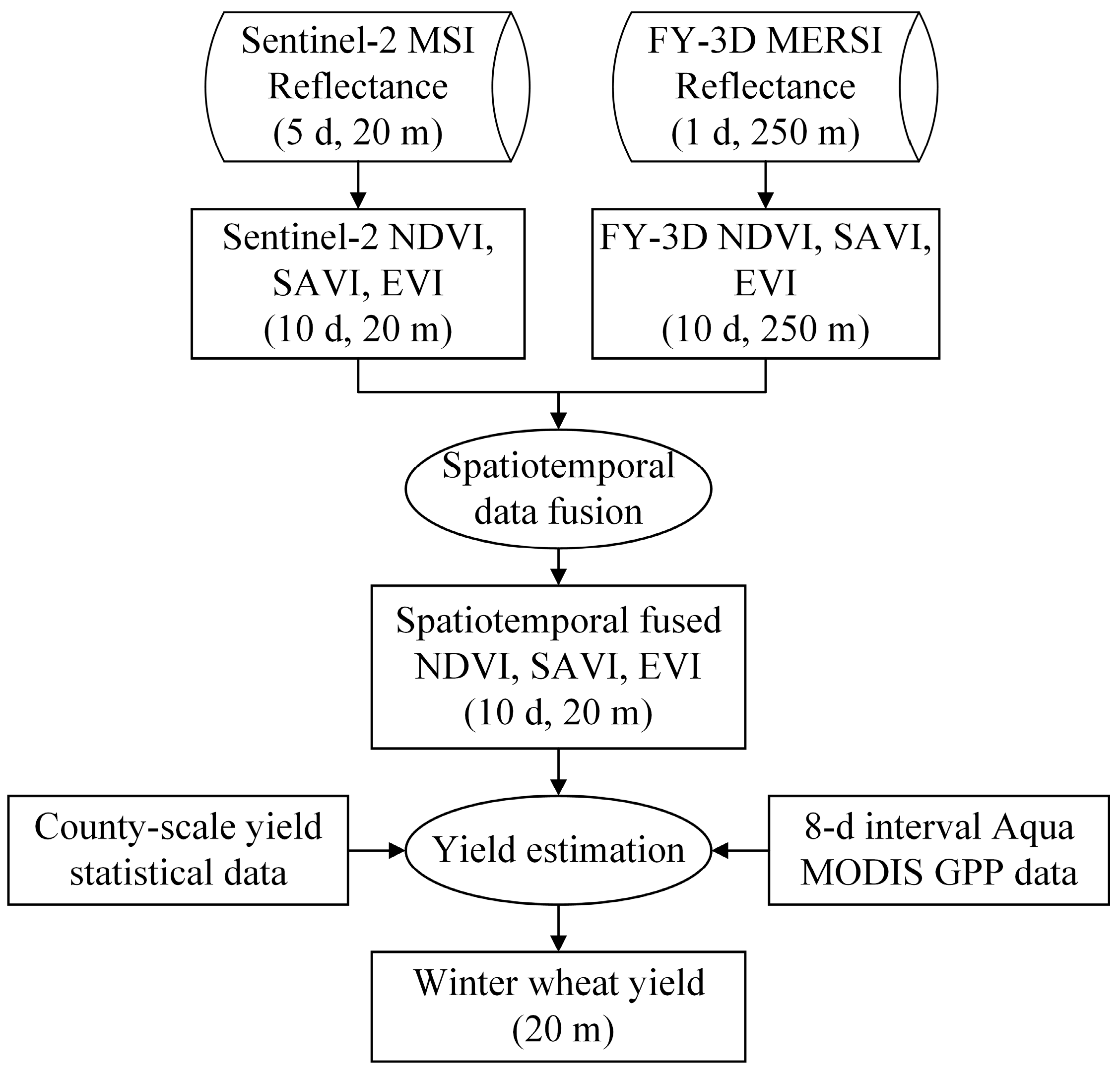
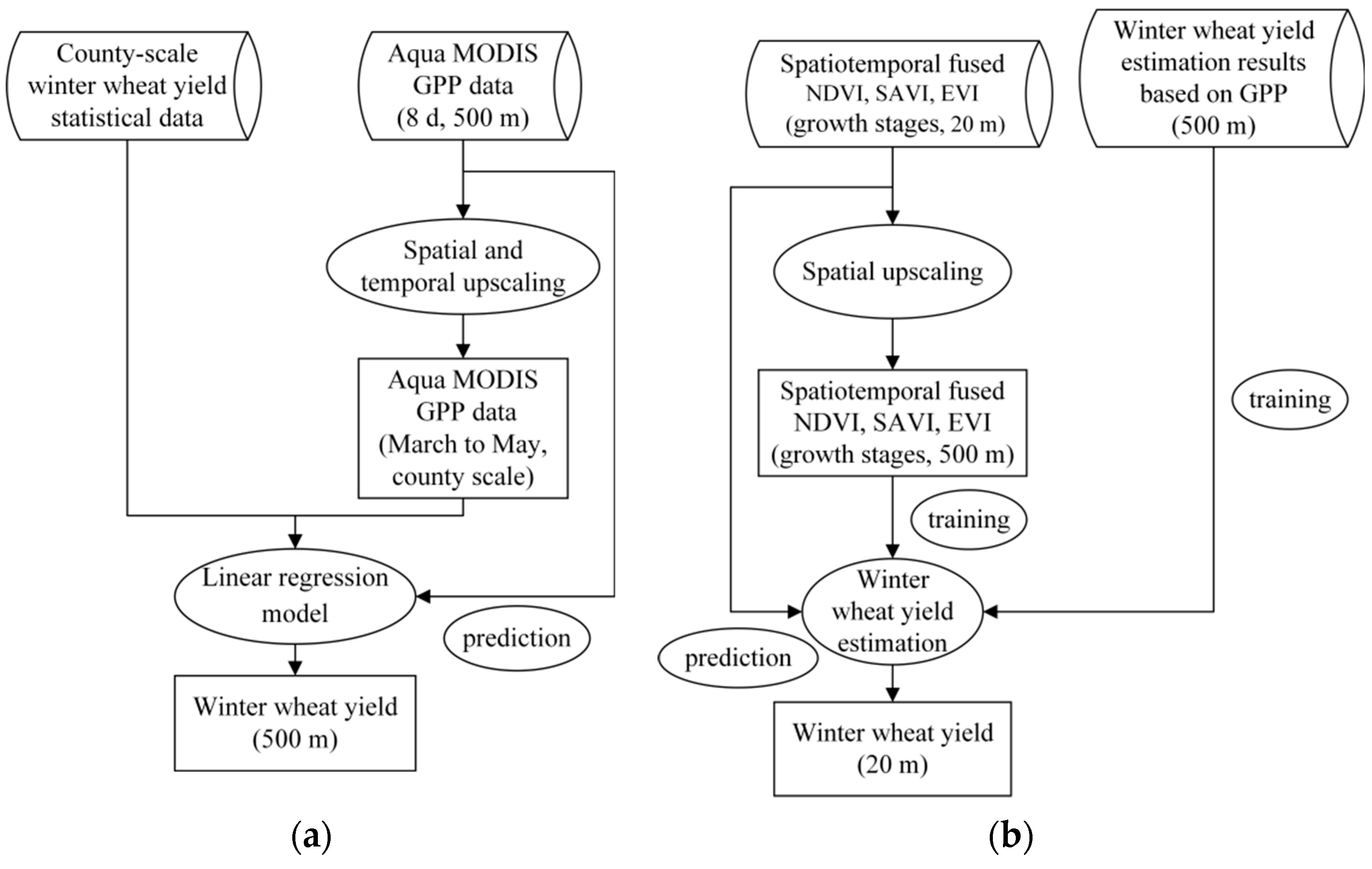

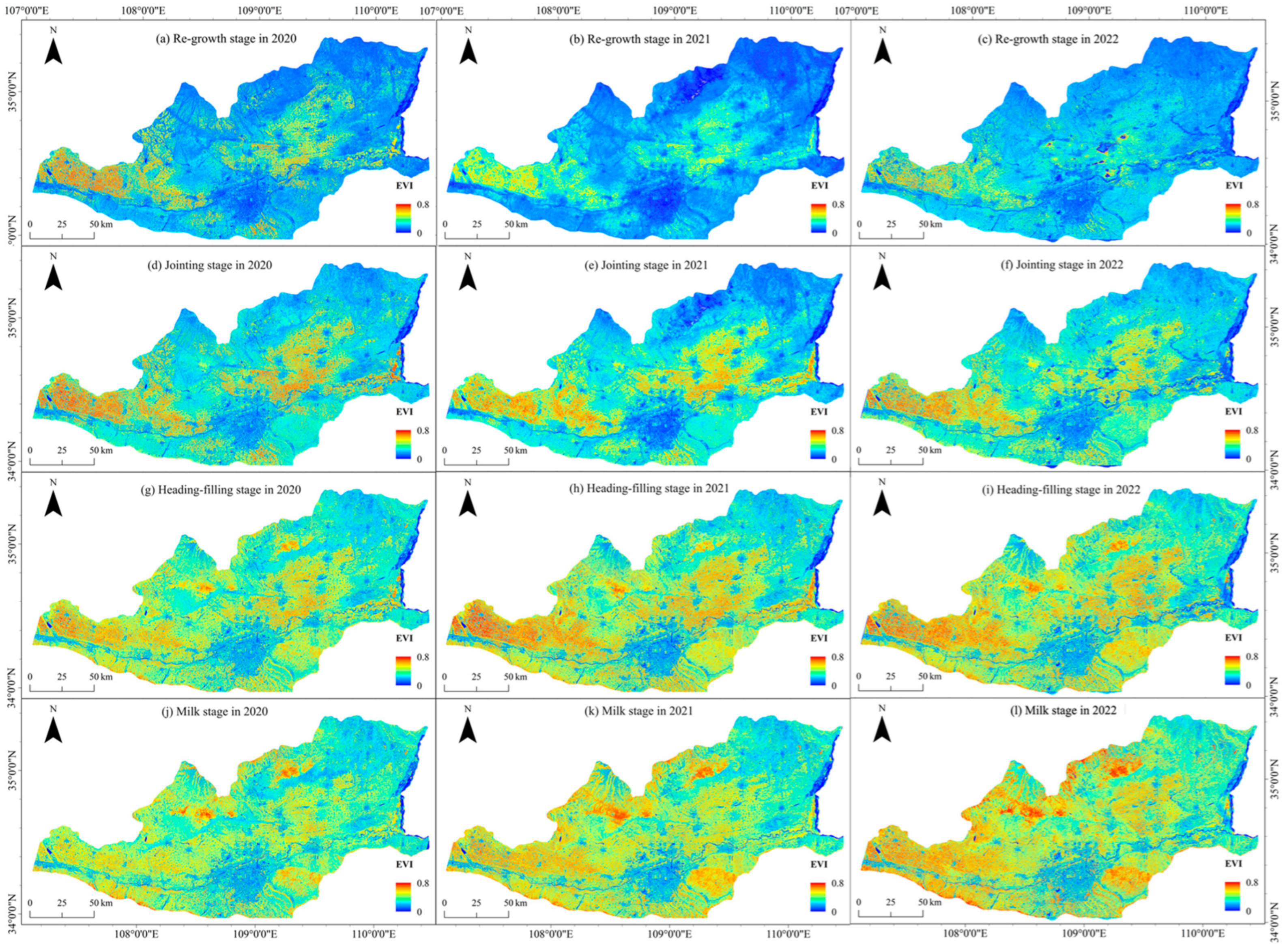
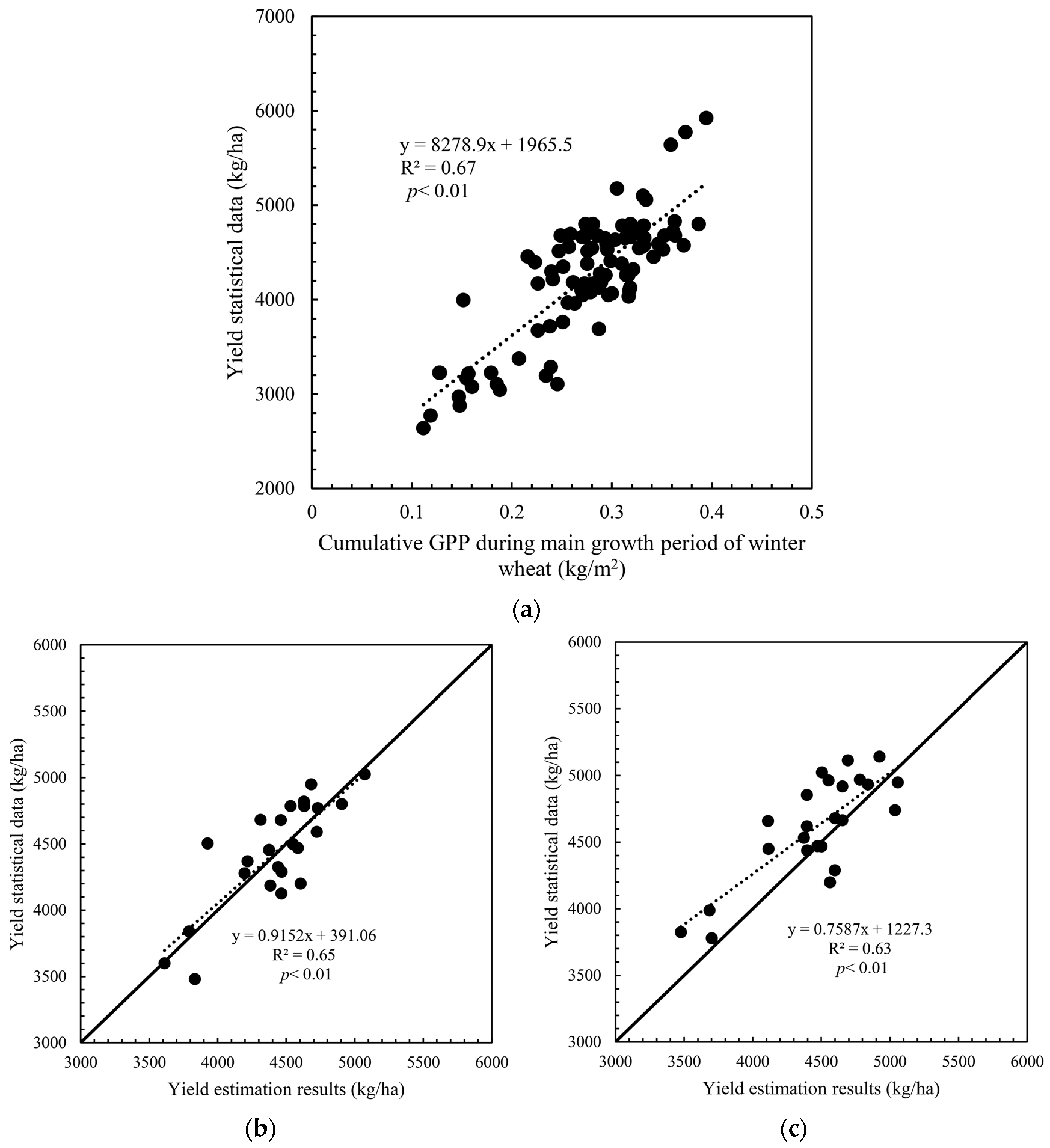
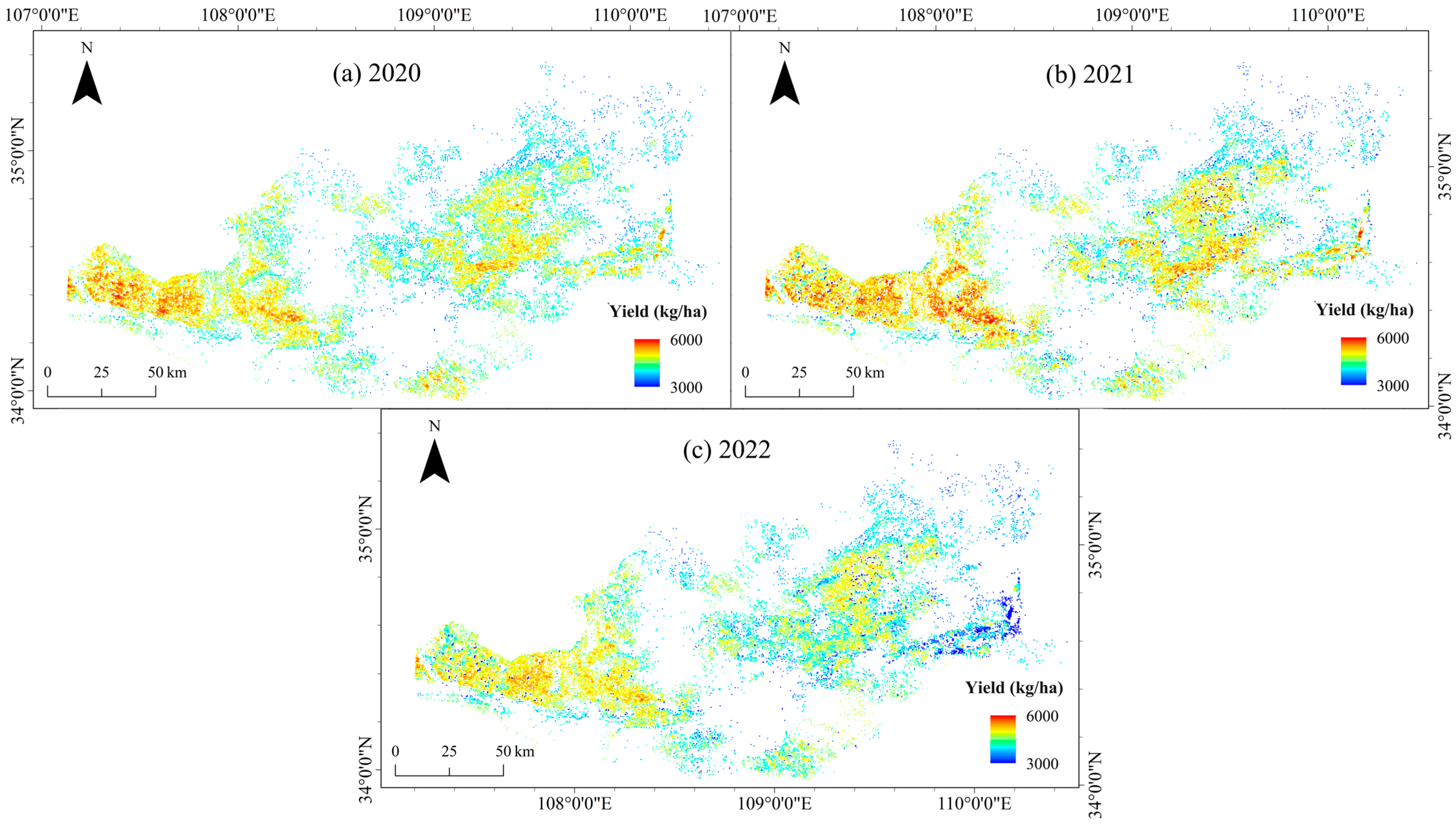
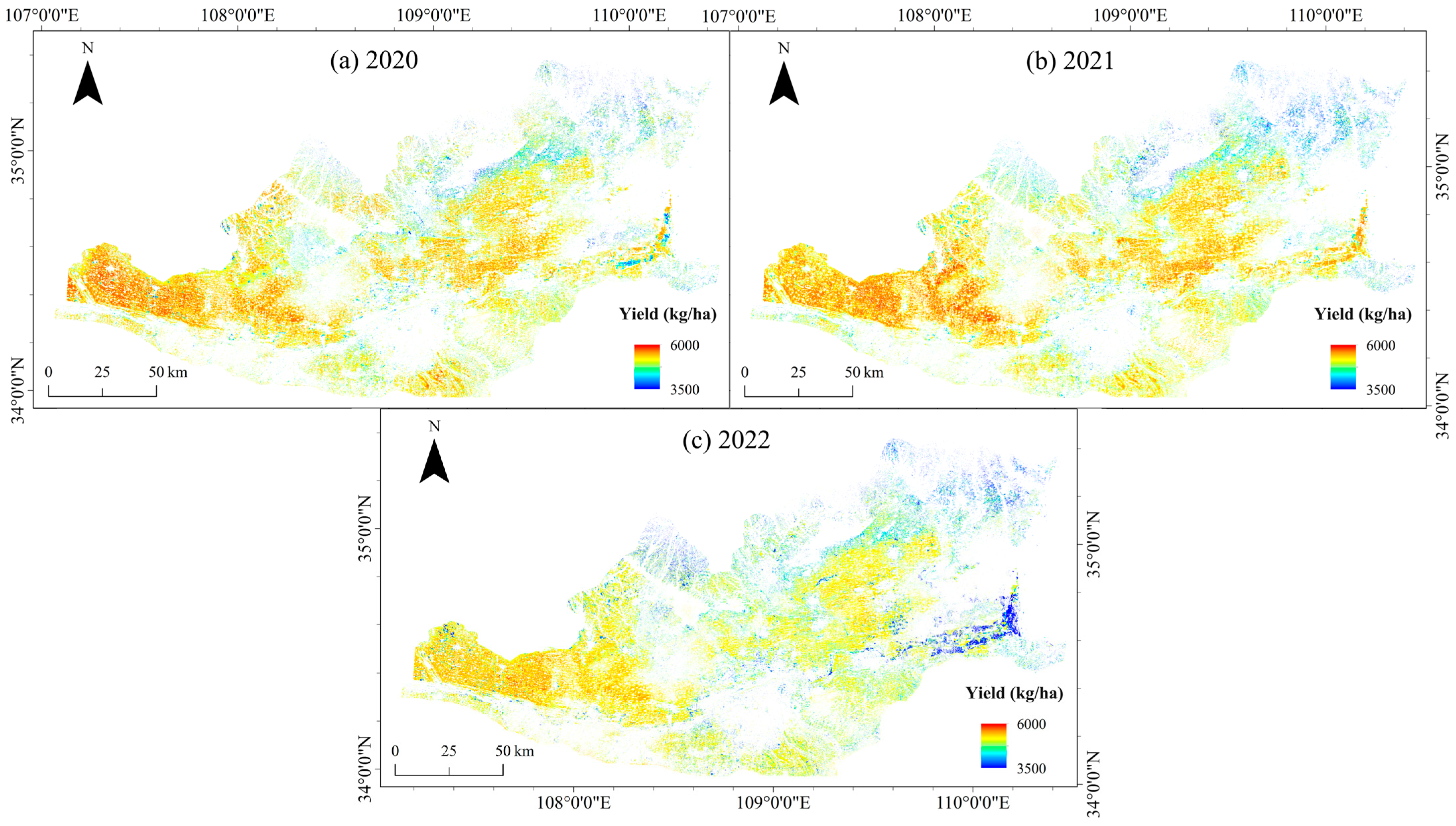
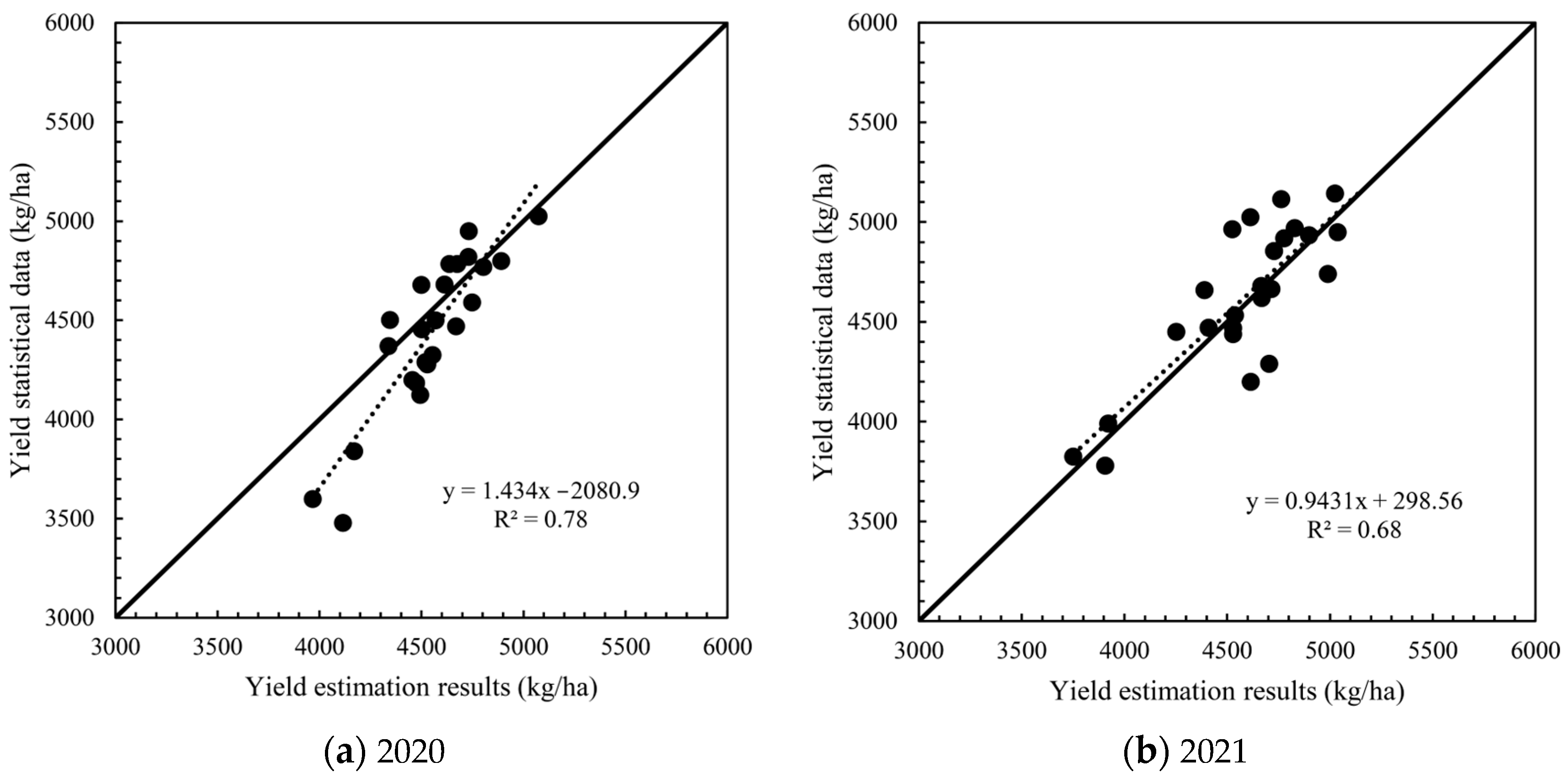
Disclaimer/Publisher’s Note: The statements, opinions and data contained in all publications are solely those of the individual author(s) and contributor(s) and not of MDPI and/or the editor(s). MDPI and/or the editor(s) disclaim responsibility for any injury to people or property resulting from any ideas, methods, instructions or products referred to in the content. |
© 2024 by the authors. Licensee MDPI, Basel, Switzerland. This article is an open access article distributed under the terms and conditions of the Creative Commons Attribution (CC BY) license (https://creativecommons.org/licenses/by/4.0/).