Abstract
Change detection (CD) identifies surface changes by analyzing bi-temporal remote sensing (RS) images of the same region and is essential for effective urban planning, ensuring the optimal allocation of resources, and supporting disaster management efforts. However, deep-learning-based CD methods struggle with background noise and pseudo-changes due to local receptive field limitations or computing resource constraints, which limits long-range dependency capture and feature integration, normally resulting in fragmented detections and high false positive rates. To address these challenges, we propose a tree topology Mamba-guided network (TTMGNet) based on Mamba architecture, which combines the Mamba architecture for effectively capturing global features, a unique tree topology structure for retaining fine local details, and a hierarchical feature fusion mechanism that enhances multi-scale feature integration and robustness against noise. Specifically, the a Tree Topology Mamba Feature Extractor (TTMFE) leverages the similarity of pixels to generate minimum spanning tree (MST) topology sequences, guiding information aggregation and transmission. This approach utilizes a Tree Topology State Space Model (TTSSM) to embed spatial and positional information while preserving the global feature extraction capability, thereby retaining local features. Subsequently, the Hierarchical Incremental Aggregation Module is utilized to gradually align and merge features from deep to shallow layers to facilitate hierarchical feature integration. Through residual connections and cross-channel attention (CCA), HIAM enhances the interaction between neighboring feature maps, ensuring that critical features are retained and effectively utilized during the fusion process, thereby enabling more accurate detection results in CD. The proposed TTMGNet achieved F1 scores of 92.31% on LEVIR-CD, 90.94% on WHU-CD, and 77.25% on CL-CD, outperforming current mainstream methods in suppressing the impact of background noise and pseudo-change and more accurately identifying change regions.
1. Introduction
Change detection (CD) is an essential research topic within the field of remote sensing (RS) and involves identifying building changes in surface structures by comparing bi-temporal remote sensing images of the same area. It is widely applied in land use monitoring [1], urban planning [2], and environmental change detection [3]. With the ongoing advancements in remote sensing technology, dual-temporal remote sensing imagery facilitates high-frequency, large-scale, and flexible-temporal-scale CD, but the imaging process is typically affected by environmental, atmospheric, and imaging conditions, leading to noise and distortions. This poses significant challenges for accurately extracting and analyzing building change information from the images. Therefore, advancing the accuracy and robustness of CD methods becomes a pressing need, especially considering the challenges introduced by various image distortions and noise.
Traditional CD methods predominantly depend on directly comparing original bi-temporal RS images or manual extraction of spectral, texture, shape, and geometric features through feature transformation from images, followed by comparing these features to identify change [4,5,6]. Due to the reliance on manual feature extraction, traditional CD methods have limited ability to perceive interference in RS imagery, which greatly influences the precision of the results. In addition, inadequate capability for high-level feature extraction further limits the accuracy of the results.
Over the past decade, Convolutional Neural Networks (CNNs) have been extensively utilized in semantic segmentation tasks [7], owing to their exceptional abilities to automatically extract high-level features and capture local spatial structures in images. CNN-based CD methods are commonly built upon Siamese structure alongside skip connections for multi-scale feature extraction and fusion, providing the capability to capture both coarse features and fine features [8,9,10]. Nevertheless, the restricted receptive field poses a limitation on global feature extraction, which remains a critical drawback for CNN-based CD methods. This shortcoming can substantially affect the detection accuracy and robustness of models [11]. Considering this limitation, Transformer [12] models have emerged as a powerful alternative, benefiting from the ability of a self-attention mechanism to capture both long-range dependencies and global contextual information. Building upon the success of the Transformer architecture in computer vision tasks [13], researchers in remote sensing have developed Transformer-based models specifically tailored to the challenges of CD. The global perspective of these models proves particularly beneficial in scenarios with extensive and intricate changes, enhancing their ability to distinguish and reduce background noise [14,15,16,17]. Nevertheless, Transformer-based models also bring certain challenges, including high computational costs and a need for large datasets to train effectively, which restrict their utility in data-limited settings [18,19]. Fortunately, the recent advent of the Mamba [20] architecture provides researchers with the promise to address the inherent limitations of Transformer-based methods. Mamba architecture builds upon the Selective State Space Model (SSM), eliminating the attention mechanism in the Transformer, thereby achieving linear time complexity. A distinguishing feature of Mamba is the selection mechanism, enabling the model to selectively retain or discard information at each time step. This strategy allows Mamba to effectively handle dense or sporadic information by preserving key data and filtering out unnecessary details. Currently, the Mamba architecture has also been transferred to the visual domain including RS tasks [21,22,23], demonstrating strong competitiveness against Transformer-based models.
Although the methods mentioned present promising results, there remains significant room for exploration in how to accurately extract feature information from remote sensing images and reduce the interference of background noise and pseudo-changes. In CD, data imbalances are a common issue, which leads to higher false predictive rates. Meanwhile, the variations in imaging angles and environments at different time points in bi-temporal images, along with the diversity of ground objects in remote sensing imagery, result in notable intraclass variations and strong interclass similarities [24], severely interfering with the identification of change areas. Currently, mainstream CD methods detect change areas by extracting and fusing multi-scale feature information. Apart from the intrinsic capabilities of models to extract features, which fundamentally affect predictive performance, the fusion of these features also plays a decisive role. Aligning and complementing features of different scale features can effectively detect key edge details of changed regions while capturing the geometric shape of the regions and providing spatial location information.
This article proposes a CD method based on Mamba architecture, composed of a Tree Topology Mamba Feature Extractor (TTMFE) and Hierarchical Incremental Aggregation Module (HIAM). In contrast to the existing Mamba method, TTMFE replaces the original SSM module with Tree Topology SSM (TTSSM), breaking the limitation of traditional Mamba that can only rely on fixed sequences for information transmission, which enhances the model’s ability to capture the long-range dependency relationships, while maintaining the advantages of global context information extraction ability of the Mamba structure, further enhancing the capability to extract local spatial and structural features. In addition, to better adapt to CD tasks, the HIAM is employed to align and fuse the multi-scale features extracted by TTM. The HIAM has effective interaction with information at different scales, ensuring that important scale features are fully utilized. The main contributions of this study are listed as follows:
- (1)
- We construct a Tree Topology Mamba Feature Extractor (TTMFE), which generates the minimum spanning tree through the similarity between pixels by a Tree Topology State Space Model (TTSSM), allowing information to be transmitted and aggregated on a tree structure to fully capture multi-scale spatial–temporal features.
- (2)
- We devise a HIAM to establish a bridge for information communication between adjacent scales, which facilitates effective multi-scale feature aggregation by enhancing the interactions between neighboring features from deeper to shallower layers.
- (3)
- We conduct an evaluation of our method across three publicly accessible change detection datasets. The experimental results demonstrate this method is very competitive and has even more state-of-the-art performance than other mainstream methods.
2. Related Works
2.1. CNN-Based CD
CNNs have shown significant effectiveness in change detection (CD) applications by harnessing their capability to extract hierarchical features and capture local spatial patterns. Over the years, various CNN-based models have been proposed to boost CD accuracy through strategies that mitigate noise, sharpen boundaries, and enhance feature fusion. As a classic illustration, Chen et al. mentioned Siamese_AUNet [25], which uses a dual-branch U-Net architecture and multi-scale pooling to capture features from input images, effectively enhancing detection accuracy by preserving fine details and mitigating background noise. In CD, combining CNN networks with attention mechanisms and feature fusion has been widely adopted, as it features representation by highlighting information in regions where changes have occurred while suppressing areas with no changes. [26]. Such an approach can successfully identify subtle variations and enhance detection performance. Hewarathna et al. incorporated an attention mechanism into the Siamese U-Net architecture to direct the model’s focus toward regions with significant changes and suppress irrelevant areas, thereby enhancing its capacity for global feature extraction and improving detection accuracy [27]. Notwithstanding that Siamese architecture, multi-scale feature fusion, and attention mechanisms enhance the global feature extraction of CNN-based methods to some extent, the inherent limitation of receptive fields hampers effective long-range dependency capture, often posing difficulties in identifying spatially distributed changes and distinguishing actual changes from background noise [28].
2.2. Transformer-Based CD
Transformer-based models have gained traction in CD tasks for their ability to capture long-range dependencies and incorporate global contextual information. These models are especially effective in identifying complex, large-scale changes and reducing background interference [29,30]. To leverage both local and global feature extraction, recent work has explored hybrid models that combine the strengths of CNNs for capturing detailed local features with the global modeling capabilities of Transformer [31]. Such architectures improve feature integration and enhance precision for high-resolution, multi-scale CD applications [32]. For example, Han et al. [33] introduced a self-attention mechanism block into the traditional U-net structure to guide the fusion of extracted multi-scale features. The experimental results of the study indicate that this method can effectively reduce edge fragmentation and internal holes. Jiang et al. [34] introduced an end-to-end model that employed a CNN–Transformer hybrid structure to refine the feature pyramid extracted by the traditional CNN network. Subsequently, a gated attention module was utilized to fuse the original and refined features, enhancing the feature integration. Ding et al. [35] proposed a joint approach for semantic CD, integrating a new Transformer-based module, SCanFormer, with CNNs to capture temporal dependencies and spatial features. Despite these advances, the attention mechanisms central to Transformers cause the computational cost to increase quadratically with input size. The high resolution of remote sensing images in CD tasks further amplifies the computational resource and memory demands [36]. Additionally, the limited availability of data in change detection datasets, coupled with the substantial data requirements of Transformer models, hinders their ability to achieve optimal performance.
2.3. Mamba-Based CD
Mamba-based models, due to their ability to overcome the high computational and memory demands of transformers while achieving strong performance in image classification and semantic segmentation tasks, have also been applied to CD [37]. To date, researchers have proposed several frameworks based on the Mamba architecture specifically adapted for CD tasks. For example, Liu et al. designed the Iterative Mamba Diffusion Change Detection model [38], which integrates a Mamba-based feature extractor with Variable State Space Change Detection to iteratively enhance feature fusion and suppress noise. Zhao et al. [39] introduced the Remote Sensing Mamba, which utilizes an Omnidirectional Selective Scan Module to improve the global context extraction capability of the model in dense prediction by scanning inputs across multiple directions. Chen et al. introduced the MambaBCD model [40], featuring a Mamba-based Siamese encoder and a Spatio-Temporal State Space (STSS) module to effectively capture spatial–temporal relationships. The STSS module uses sequential, cross, and parallel modeling to enhance feature interaction, enabling superior performance across benchmark datasets while maintaining efficiency. The results from these studies demonstrate the feasibility and significant promise of the Mamba architecture in CD. However, many methods apply fixed scanning templates in SSM or the combination of certain fixed scanning methods, which limits the ability to preserve spatial structural information, leading to discontinuities and loss of critical local features, thereby hindering the effective identification of subtle pseudo-changes caused by environmental variations [41].
3. Methods
This section describes the overview framework and introduces each subnetwork, including the feature extraction module, feature fusion module, and loss function.
3.1. Overview
In CD tasks, the comprehensive extraction of boundary position features is essential for accurately identifying areas of change. However, existing Mamba-based models typically rely on simplistic directional or fixed-template scanning methods such as General Raster Scan [42], Continuous Scan [43], and Diagonal Scan. This limitation impedes the model’s ability to effectively extract position relationships, resulting in poor generalization capabilities and challenges when processing complex and dynamic remote sensing images. Additionally, insufficient information interaction between features at different scales may result in the loss of important feature information during the feature fusion process, thereby impeding the further capture of feature details and contextual relationships.
To overcome these challenges, we propose TTMGNet for CD tasks. The TTMGNet consists of two components, TTMFE and HIAM, as illustrated in Figure 1. TTMFE is a multi-stage structure based on Mamba architecture, featuring two branch networks with shared weights, designed for feature extraction from input bi-temporal images of the same pattern: Ipre and Ipost, where Ipre represents the earlier time-series image and Ipost denotes the subsequent time-series image of the same area. TTMFE includes a stem module followed by four feature extraction stages containing 3, 4, 18, and 5 TTM blocks, respectively. Each TTM block is a Mamba-based architecture with TTSSM, specifically designed to enhance feature extraction for CD tasks. This configuration enables the generation of multi-scale feature maps that progressively capture both global and local contexts. Initially, the input image passes through the stem module for preliminary feature extraction and downsampling. The generated feature map is then sent to the first feature extraction stage, undergoing further feature extraction, followed by downsampling to halve the spatial dimensions and double the channel count. The subsequent three feature extraction stages follow the same process. After the final stage, feature maps from each branch are concatenated at the same scale, yielding four multi-scale feature maps as input for HIAM. The HIAM is constructed to efficiently merge the multi-scale feature maps produced by TTMFE, focusing on enhancing significant features, suppressing redundant information, and preventing critical feature loss during fusion. HIAM performs fusion hierarchically, progressively combining feature maps at different scales to form a rich representation tailored for change detection. The key components of HIAM are cross-channel attention (CCA) and residual connections. The CCA module aligns features across adjacent levels, moving from deeper layers, which capture broader contextual information, to shallower layers containing finer details, enhancing the capacity of the model to identify subtle changes. Residual connections are integrated throughout HIAM, maintaining original features during fusion while helping preserve complex global dependencies alongside local details.
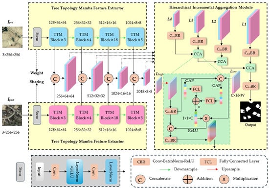
Figure 1.
The overview flow diagram of TTMGNet, where σ represents the sigmoid activation function and GAP denotes the Global Average Pooling operation. The data flow begins with the bi-temporal images, Ipre and Ipost, which are fed into the stem module. Subsequently, the extracted features undergo further extraction through four stages within the TTMFE, each consisting of a different number of TTM blocks. Finally, the outputs from all four stages are then fed into the HIAM for feature alignment and fusion, ultimately generating the final output image.
3.2. Tree Topology Mamba Feature Extractor
The Tree Topology Mamba Feature Extractor is a Siamese network comprising four distinct stages, utilizing two RGB remote sensing images as input, which represent images of the same area captured at different times.
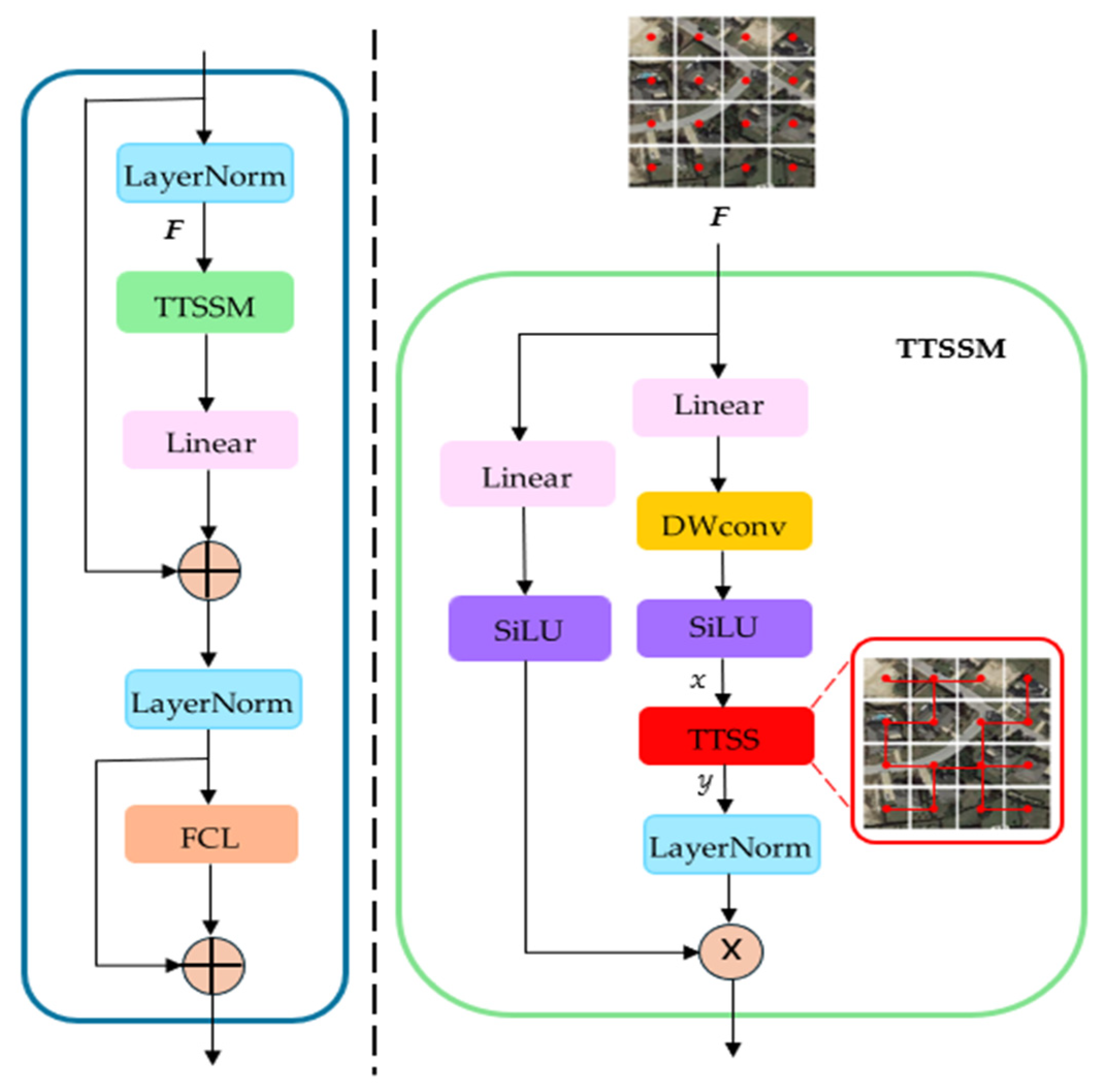
In Figure 1, the input images are first processed through a stem module composed of 2D Convolution layers for preliminary feature extraction, followed by further extraction using the TTM block. In different stages, the input is initially processed by convolution to reduce its size while increasing the number of channels, and then various TTM blocks are employed for feature extraction. The structure of the TTM is like the original Mamba structure, which is demonstrated in Figure 2, encompassing linear layers, a depth-wise convolution layer, and a Tree Topology State Space Model (TTSSM) block. Additionally, skip connections serve to stabilize training and improve performance, with an FCL at the end for further feature refinement. Given that the Mamba structure extracts feature information solely through scanning the sequences obtained from the inputs, the scanning method significantly influences the feature extraction capabilities. We employ the TTSSM to replace the original SSM, enabling a variable scanning mode to accommodate different inputs, thereby enhancing the model’s generalization ability and improving its capacity for global information extraction. Based on the architecture described, the entire process can be formulated as follows:
where denotes the input feature i-th stage, C, H, and W represent channel number, height, and width, respectively, donates the output of the i-th stage, Down means doubling the number of input channels and reducing the size by a factor of two, and means the number of TTM blocks in the i-th stage; the TTM can be formulated as follows:
where means the input of the current TTM block, Linear denotes linear layer, LN is layer normalization, represents the element-wise multiplication of matrix, and indicate intermediate results, SiLU is the activation function, DWconv is a depth-wise convolution layer, MLP means Multilayer Perceptron, and FCL denotes a fully connected layer.

Figure 2.
The inner structure of the TTM block, where F is the input feature of the TTSSM module, the red points in F indicate pixels, MST denotes the minimum spanning tree composed of pixels, and x and y mean the input and output of the TTSS block. Details of TTSS are shown in Figure 3.
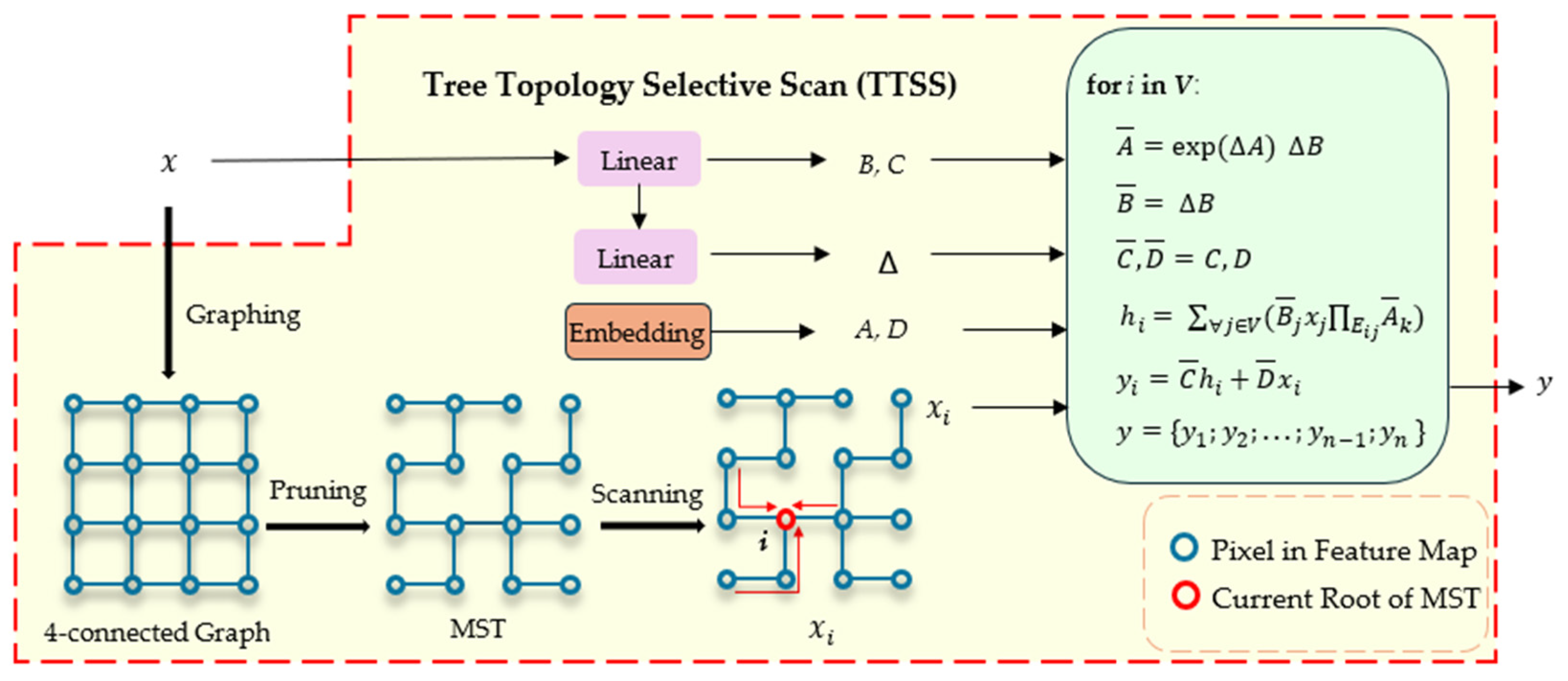
Tree Topology Selective Scan is the core component of the TTSSM. The workflow of TTSS is shown in Figure 3. In TTSS, each pixel of the input feature map is treated as a vertex, and a 4-connected graph is constructed by connecting each vertex to its four directly adjacent vertices. The edge weights in the graph are computed based on the feature similarity between the two connected vertices, where the similarity is measured using cosine similarity. Subsequently, pruning is applied to remove edges with larger weights until a minimum spanning tree (MST) is formed, which is the MST in Figure 3. Then, we apply the BFS algorithm on the MST to generate a sequence and sequentially set each node as the root node of the tree according to this order. Through the MST, the state transition function [44] is used to propagate and aggregate information between all nodes, eventually updating the feature values of each vertex. This approach maximizes the capture of global contextual information, while the tree structure, by establishing connections between pixels with high similarity, effectively preserves local detailed features. This is an advantage that traditional fixed scanning methods in SSM do not possess. For the state transition function, A is the state transition parameter, B is the input mapping parameter, C is the output mapping parameter, and D is the direct input–output mapping parameter. is used to transform the continuous parameters into discrete equivalents, enabling the discretization of continuous State Space Models to handle the discrete input data typically found in tasks such as visual processing.
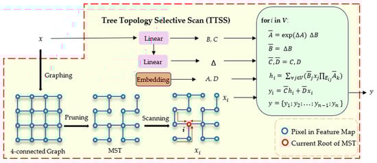
Figure 3.
The illustration of TTSS. A, B, C, and D are the parameters of the TTSSM, means the transform parameters used to discrete the continuous parameters of A and B. Set V means all vertices in MST, denotes all edges from vertex to vertex j. means the transition parameters of vertex k. is the hidden state of the input.
3.3. Hierarchical Incremental Aggregation Module
Multi-scale feature extraction is widely used in CD tasks, as this structure can more comprehensively capture detailed information in images. Therefore, effectively integrating features from different scales has become a critical challenge in CD. Insufficient interaction between features at different scales can result in the loss of critical details, significantly reducing the model’s ability to identify areas of change. To address this, we propose the Hierarchical Incremental Aggregation Module (HIAM) to facilitate feature fusion. The overview of the HIAM is displayed in Figure 1. The HIAM progressively fuses adjacent feature levels from deep to shallow layers, employing multiple skip connections to enhance information interaction between different layers. Additionally, cross-channel attention [45] is utilized to further strengthen the complementary nature of the information across layers, while emphasizing important features. This ensures that these key features are more effectively utilized, thereby improving the overall efficacy of multi-scale feature integration. As shown in Figure 1, L1, L2, L3, and L4 represent the extracted feature from deep to low separately; we first adopt a convolution layer with stride = 1 and padding = 1 to refine the local features, followed by a Batch Normalization layer and a ReLU activation layer.
where indicates the input feature map, denotes convolution operation, BN refers to Batch Normalization, and ReLU represents the activation function, referring to CBR in Figure 1. Next, the CCA module is incorporated to perform feature fusion between two neighboring layer features. The CCA module has two inputs, and , where means the high-level feature map and means the low-level feature map:
where CCA denotes the CCA module. According to Figure 1, the CCA module can be formulated as follows:
where UP represents an upsampling operation, Concat means a concatenation operation, illustrates the weight of the different channels, GAP refers to Global Average Pooling, and indicates a sigmoid activation function. We apply a CRB block where C is to both and and then perform concatenation across the channel axis. We apply cross-channel attention to derive the weights for the features across different channels and obtain the new feature map by multiplying and . Finally, we use a skip connection between and to mitigate the information loss caused by feature fusion and obtain the final fused features through a CBR block. The entire process can be formulated as follows:
3.4. Loss Function
The datasets used for CD tasks typically exhibit a significant imbalance between foreground and background pixel quantities. Dice Loss is suitable for binary image segmentation tasks. In the context of CD tasks, it optimizes the similarity between the model’s predicted change regions and the actual change regions, thereby improving detection accuracy. For binary classification tasks, Dice Loss can be calculated as follows:
where H and W represent the height and width of the input images, respectively, means the predicted value of the pixel at coordinates , indicates the true value of the pixel located at position .
Binary Cross-Entropy (BCE) Loss is a widely adopted loss function for binary classification problems; it optimizes the performance of models by minimizing the cross-entropy between the predicted values and the true labels. BCE Loss can be calculated using the following formula:
where the meanings of H, W, , and are the same as in . For our method, we employ a combination of Dice Loss and BCE Loss, which is
4. Experiments and Result Discussion
This section introduces the parameter settings, datasets, and evaluation metrics used in the experiments. In addition, this section presents the results of our method on different datasets and provides a comparison and analysis of the performance with other methods.
4.1. Dataset
To verify the feasibility of our method, we conducted experiments on three different CD datasets, as detailed in the following:
- (1)
- The LEVIR-CD [46] dataset has 637 pairs of ultra-high-resolution RS images, each measuring 1024 × 1024 pixels with a spatial resolution of 0.5 m per pixel. This dataset was proposed by Bei-hang University from Google Earth, capturing land use changes over a duration ranging from 5 to 14 years, primarily focusing on land use change, which includes residential villas, high-rise apartments, garages, and warehouses. To facilitate model training, the original images were divided into segments of 256 × 256 pixels. After the removal of duplicate portions, the dataset contains 4449 pairs of 256 × 256 dual-temporal images, with the number of images designated for training, validation, and testing being 3096, 432, and 921, respectively.
- (2)
- The WHU-CD [47] dataset consists of a pair of high-resolution images measuring 0.75 m, with dimensions of 15,354 × 32,507 pixels, covering an area of 450 square kilometers in Christchurch, New Zealand. The dataset was obtained through aerial photography in 2012 and documents land use changes in Christchurch following the 2011 earthquake. The full image was divided into 7432 image pairs, each with a resolution of 256 × 256 pixels, with a training, validation, and testing set ratio of 7:1:2, resulting in 5201, 744, and 1487 images, respectively.
- (3)
- The CL-CD [48] dataset consists of 600 pairs of bi-temporal images with a resolution of 512 × 512 pixels and a spatial resolution ranging from 0.5 to 2 m. The images were collected in 2017 and 2019 by satellite over cropland areas in Guangdong Province for cropland CD. We divided this dataset into 360, 120, and 120 pairs of images for training, validation, and testing.
4.2. Implementation Details
We used the PyTorch deep learning framework to implement all the models in our experiments, and all training work was conducted on a single NVIDIA Tesla A100 GPU. For the specific parameter settings in our model, the batch size was configured to 32, and the training process was run for 500 epochs. The AdamW optimizer was employed with an initial learning rate of 0.00035 and a weight decay set to 0.001. Additionally, a cyclic cosine annealing learning rate schedule was used to accelerate the convergence and enhance the model’s stability. For the training period, we applied several augmentation techniques to increase dataset diversity and improve model robustness, including random flips, rotations, translations, cutouts, and HSV adjustments. Additionally, histogram equalization and Gaussian blurring were used. During inference, only normalization, resizing, and histogram matching were used. The source code is available at https://github.com/COMPHZ/TTMGNet. We also employed a validation set and early stopping to prevent the overfitting of the model. For performance evaluation, we selected six metrics: Precision, Recall, F1 score, Overall Accuracy (OA), mean Intersection Over Union (mIOU), and Kappa coefficient, which are calculated by the following formulas:
where TP denotes correct positive class prediction, FP indicates incorrect positive class prediction, TN refers to correct negative class prediction, and FN is incorrect negative class prediction. is the proportion of correctly classified samples out of the total samples, with a calculation identical to that of OA. is the expected accuracy.
To showcase the effectiveness of the proposed method, we performed comparative experiments using eight models on the LEVIR-CD, WHU-CD, and CL-CD datasets, based on the metrics mentioned above and visualization results. The compared models include FC-EF [46], BITNet [49], HFANet [50], MSCANet [48], DMINet [51], SARASNet [52], Went [53], and CSINet [54].
4.3. Results and Visualization on LEVIR-CD
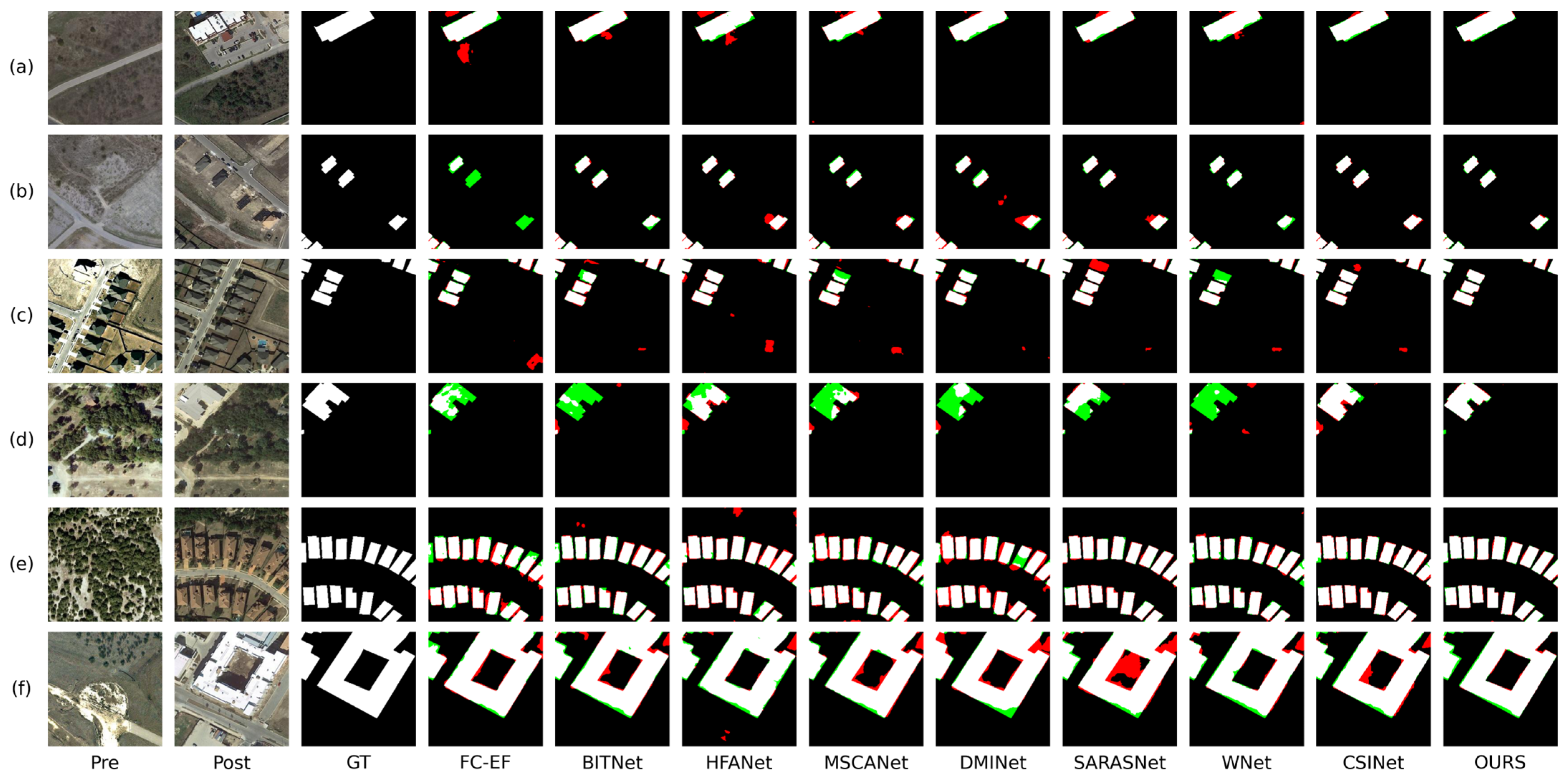
The LEVIR-CD dataset is widely used in building CD; we perform a visual comparison of the proposed method against other approaches across six specific scenarios from the LEVIR-CD dataset, as illustrated in Figure 4. As shown in Figure 4a, due to the high similarity between the surface material in the upper-left corner and the building surface, most methods mistakenly detect this area as a change region. In addition, due to the significant color difference between the building’s edges and its main body, most models regard this area as a non-change region. Our approach handles these two cases more effectively, achieving the lowest probabilities of missing detections and false detections. As shown in Figure 4b, due to the high similarity between the building color and the surface color, HFANet, WNet, and BITNet exhibit large-scale missed detections. Furthermore, HFANet, DMINet, and SARASNet are significantly affected by shadows, mistakenly detecting shadowed areas as building change regions. In comparison, our method achieves more accurate localization of building change regions. As shown in Figure 4c, the significant intraclass differences caused by variations in lighting intensity and shooting angle have caused significant interference with most methods. All methods except for our method have experienced a certain degree of missed and false detections. As shown in Figure 4d, apart from CSINet and our method, all methods exhibit significant missed detections. This issue arises from the high similarity between the background color and the building color. As shown in Figure 4e, FC-EF, HAFNet, MSCANet, and MDINet are heavily affected by the interference of building shadows, mistakenly detecting the shadowed parts at the edges of the change region as change areas. Although SARAS-Net and MAMI correctly identified the main body of the change region, there were still significant false detections and missed detections at the edges. In contrast, our model accurately identified the edges of the change region and precisely distinguished the subtle differences between adjacent pixels. As shown in Figure 4f, because of the significant difference in color between the surface in the upper right corner and the surrounding shadows and other ground surfaces, all comparison methods consider this area as a building, and only our method correctly identifies this region. The above results indicate that our method has stronger resistance to environmental noise and pseudo-change compared to other methods.
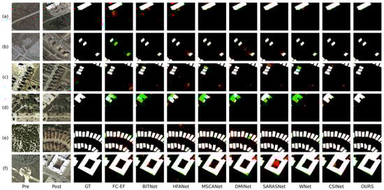
Figure 4.
Visual comparison results on the LEVIR-CD dataset. The red indicates false positives; the green indicates false negatives. (a–f) are six representative scenarios in LEVIR-CD.
To validate the outstanding performance of the proposed TTMGNet, we perform a comprehensive quantitative evaluation in comparison with the mainstream CNNs and Transformer-based networks on the LEVIR-CD dataset. Based on the results in Table 1, our method outperforms other methods across all metrics except for the Recall metric. The Recall metric is an indicator of the sensitivity of the model to identifying change areas. CSINet and SARASNet have the highest and second-highest Recall values, indicating the strong sensitivity to change regions, but both exhibit significantly lower Precision measured against TTMGNet, which suggests that the two models have a high false positive rate. Our method achieved an F1 score of 92.31%, which is considerably higher than the 91.04% achieved by CSINet, the second-best method. This indicates that our method strikes an excellent balance between Precision and Recall, effectively detecting change regions while maintaining a low false detection rate. This can be attributed to the joint use of TTMFE and HIAM, which effectively overcomes the challenge of distinguishing between natural environment changes and subtle building changes in the LEVIR-CD dataset.

Table 1.
Quantitative evaluation metrics on the LEVIR-CD against the comparison methods.
4.4. Results and Visualization on WHU-CD
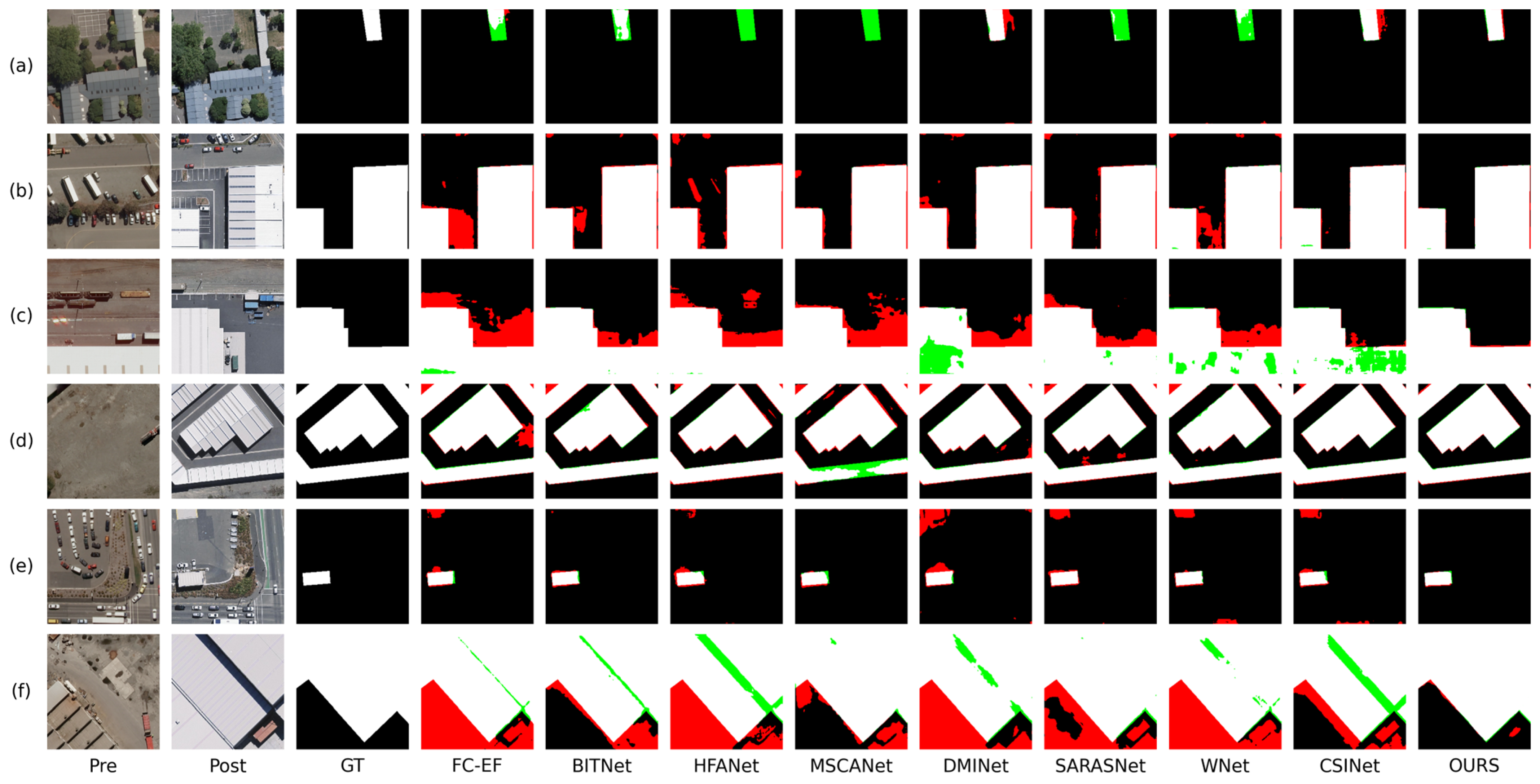
WHU-CD aims at building CD. We conduct a visual comparison between the proposed method and other methods in six specific scenarios from the WHU-CD dataset, as shown in Figure 5. As shown in Figure 5a, except for DMINet, CSINet, and our method, the methods considered are almost unable to identify the changed area due to the high similarity between the ground surface after demolishing the building and the original building roof caused by changes in lighting. However, DMINet and CSINet have large areas of false positives at the edges of the change region. Only our method can best identify the correct areas of change. As shown in Figure 5b, except for CSINet and our method, all methods exhibit varying degrees of false detections, caused by vehicle movement and surface material changes. For CSINet, the different materials on the building roofs result in color variations, leading to partially missed detections. Our model more accurately identifies the edges of building change regions, with only minimal missed and false detections. As shown in Figure 5c, the movement of ground objects and changes in roads introduce interference for most methods, with these pseudo-changes being misclassified as building changes. Furthermore, due to the minimal differences in material and texture between new and old buildings, CSINet, WNet, and DMINet exhibit large-scale missed detections. In contrast, our method only shows minimal missed and false detection areas along the edges. As shown in Figure 5d, all methods, excluding ours, misclassify non-building structures with high similarity to building surfaces as new buildings, indicating that these methods fail to overcome the challenge of small interclass differences. In contrast, our method accurately identified the changing areas and displayed fine-grained boundaries. This demonstrates that our approach possesses strong robustness against environmental interference and can precisely classify highly similar objects. As shown in Figure 5e, only BITNet, MSCANet, and our method correctly avoid misjudging the bright white surface structure in the top-left area of the image. However, BITNet and MSCANet make numerous misjudgments in the shadowed areas surrounding the buildings, failing to accurately capture the boundaries of the change regions. As shown in Figure 5f, on account of the lighting angle, a strip-shaped shadow appears in the center of the change region, creating a clear contrast with the rest of the change area and causing the loss of its original texture features. Many models are severely misled by this interference, resulting in the strip-shaped area being missed as a non-change region. Although MSCANet and SARASNet are less affected by this, they fail to overcome the influence of false changes in the lower part of the image, leading to large-scale false detections. Our model effectively avoids these two types of interference and accurately identifies the change region.
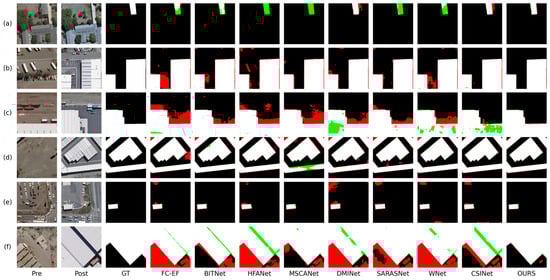
Figure 5.
Visual comparison results on the WHU-CD dataset. The red indicates false positives; the green indicates false negatives. (a–f) are six representative scenarios in WHU-CD.
We conducted a quantitative comparison of our method against the current state-of-the-art CD methods on the WHU-CD dataset. Furthermore, we performed a detailed analysis of the comparative results to demonstrate the effectiveness of our proposed method. The F1 score, which is the harmonic mean of Precision and Recall, is the most critical metric for binary CD tasks. As shown in Table 2, our method reaches an F1 score of 90.91%, surpassing the second-best method, CSINet, which has an F1 score of 88.81%. Although the Recall of our method is 1.76% lower by contrast with CSINet, the Precision is 5.9% higher, leading to the highest F1 score. Additionally, our method also obtains the highest scores in OA, mIoU, and Kappa metrics, which implies that the proposed method has the best overall classification ability, enabling it to better address the issue caused by minimal interclass differences and maximal intraclass differences. Although WNet achieved the highest Recall score of 94.98%, its performance in other metrics is significantly lower than that of our method, with the Precision metric showing the most noticeable gap, trailing our method by 20.67%.
Table 2.
Quantitative evaluation metrics on the WHU-CD against the comparison methods.
4.5. Results and Visualization on CL-CD
CL-CD focuses on cropland CD and includes complex and subtle types of changes; cropland is more susceptible to environmental variations such as seasonal and weather changes, leading to poorer performance of various methods in comparison with building CD datasets. In Figure 6, we display the visual outcomes of the proposed method and various popular CD networks.
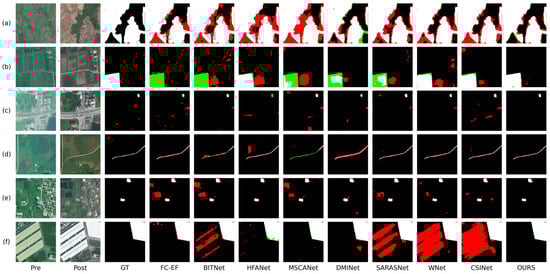
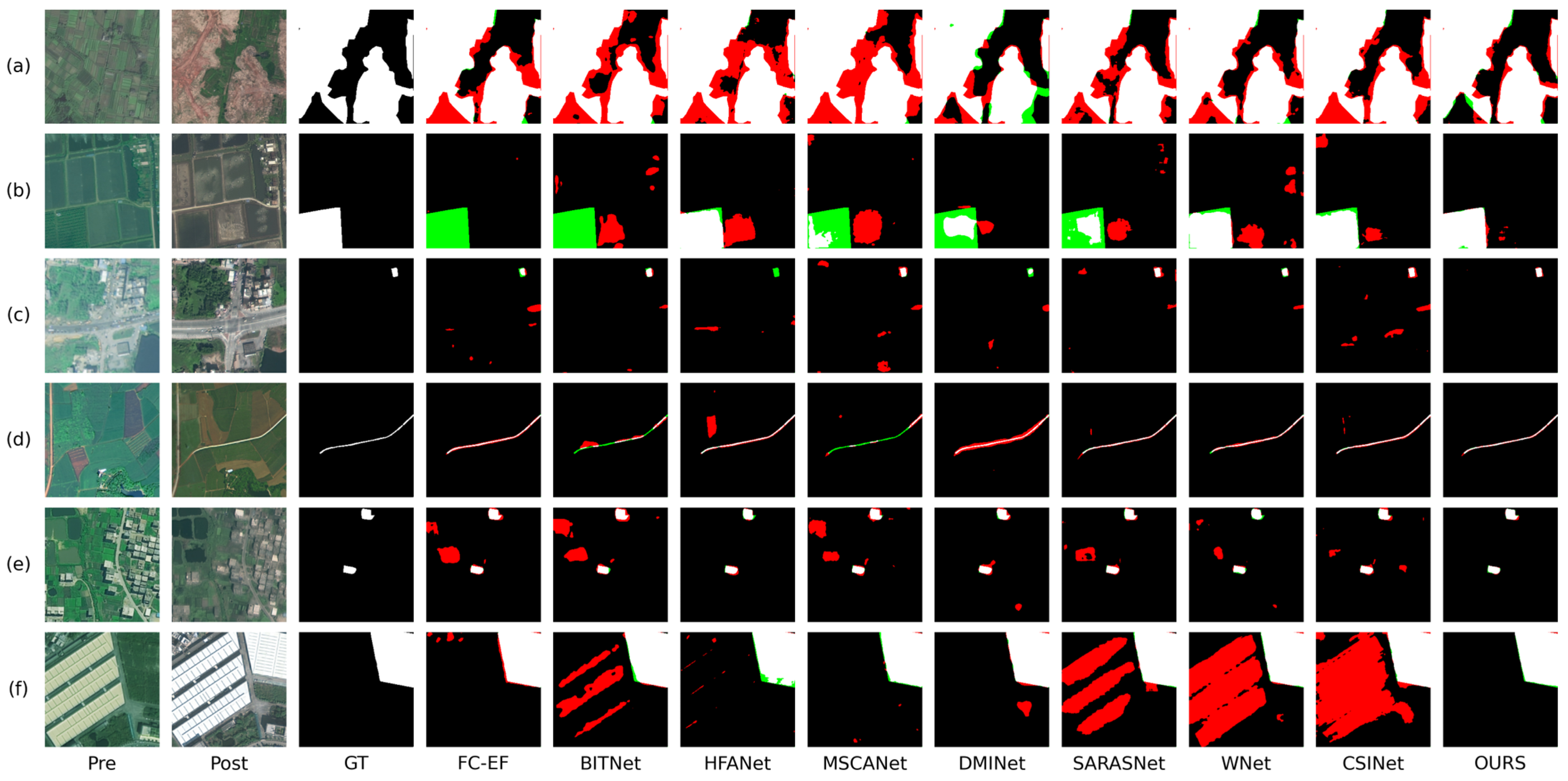
Figure 6.
Visual comparison results on the CL-CD dataset. The red indicates false positives; the green indicates false negatives. (a–f) are six representative scenarios in CL-CD.
Figure 6 presents six representative CD scenarios from the CL-CD dataset. As shown in Figure 6a, due to the high similarity between the boundaries of the change region and the background, most methods fail to accurately detect the boundaries of the change regions. Additionally, the exposed soil and vegetation loss create significant confusion with the changed regions, leading to false detections in most methods. For example, in the bottom-left corner of the image, the vegetation loss is incorrectly detected as a cropland change by most methods. Although TTMGNet also exhibits some false detections and missed detections, it performs significantly better than other methods in accurately identifying the correct CD boundaries. It is worth noting that TTMGNet effectively avoids false detections of non-cropland change regions with high similarity to the actual change regions due to environmental factors. As shown in Figure 6b, most models experience significant missed detections in the change regions because of the high similarity between crop pixels in the changed cropland areas and the original vegetation. Although WNet and CSINet can identify the contours of the changed regions to some extent, they still suffer from numerous false detections along the boundaries. Our method further sharpens the edges, resulting in fewer false and missed detections in the boundary areas. As shown in Figure 6c, the change and non-change regions are highly imbalanced. Additionally, variations in viewing angles cause the size and direction of shadows in the same forest area to change. All methods, except ours, misclassify the shadowed areas as cropland change. As shown in Figure 6d, the change region consists of elongated roads widened between multiple farmlands, posing a significant challenge to a network’s ability to extract fine-grained details. FC-EF, DMINet, and WNet exhibit numerous false detections along the road edges. Additionally, HAFNet, SARASNet, and CSINet are affected by vegetation changes within the crops, leading to misjudgments. Only our method effectively extracts the boundary information of the roads. As shown in Figure 6e, vegetation changes in the paddy fields lead to false detections in most models. Only HAFNet, DMINet, and our method successfully detect these changes; however, HAFNet and DMINet perform poorly in boundary handling, exhibiting numerous missed and false detections. As shown in Figure 6f, owing to the interference of imaging discrepancies, BITNet, SARASNet, WNet, and CSINet completely regard the large building on the left as a cropland change region. Compared with other methods, the proposed method identifies boundaries with greater sharpness, while also reducing the occurrence of false and missed detections.
The proposed method is validated through a comprehensive comparative quantitative assessment against eight mainstream methods in the field of CD utilizing the CL-CD dataset; the outcomes are presented in Table 3. CL-CD focuses on cropland CD, which is more susceptible to environmental variations, leading to poorer performance of various methods compared to building CD. According to the results, the proposed method achieves the highest scores in all metrics except for Recall, with the most significant improvements observed in Precision and F1 score, exceeding the second-best method by 4.66% and 3.52%, respectively. This is attributed to the method’s exceptional capability for contextual relationship extraction and deep detail capture. Although CSINet and HFANet have high Recall scores, their overall performance is substantially inferior to TTMGNet.
Table 3.
Quantitative evaluation metrics on the CL-CD against the comparison methods.
4.6. Stability and Ablation Analysis
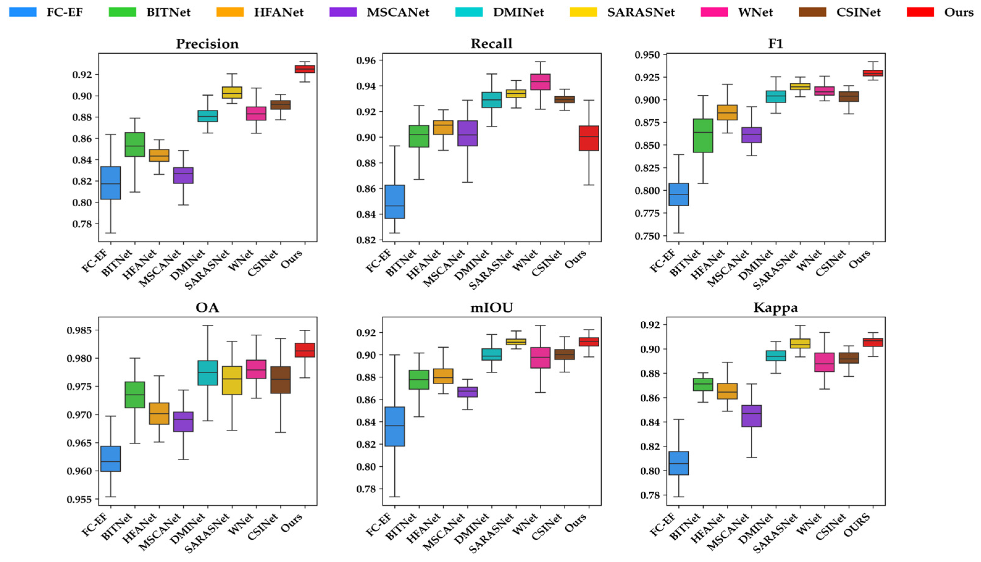
To more intuitively demonstrate the distribution of data across different metrics for various methods, we conducted a deeper quantitative analysis on the test set of the LEV-IR-CD dataset, which consists of 921 images. Six evaluation metrics were calculated individually for each image, and a more transparent comparison of the methods’ performance was provided through box plots. As illustrated in Figure 7, while our Recall metric is marginally lower as compared with SARASNet, DMINet, WNet, and CSINet, our method significantly outperforms the other eight methods compared across the remaining metrics, with Precision and F1 scores standing out, surpassing the second-best by nearly 2%. Moreover, the more compact distribution of the various metrics in our method further highlights its robustness, demonstrating the superior performance of our approach in CD tasks.
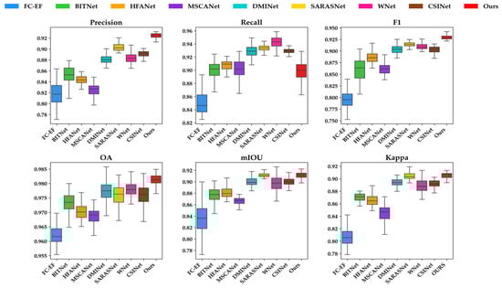
Figure 7.
Box plots of the six metrics on LEVIR-CD for the proposed method and comparison methods.
To verify the effectiveness of TTMGNet and its modules, ablation experiments were conducted on the LEVIR-CD dataset. We first replaced the TTM blocks in the TTMFE and HIAM with two modules entirely composed of CNNs and set the modified network as our baseline for testing. Subsequently, we replaced the TTM block and HIAM in sequence for testing. The results of the experiment are shown in Table 4. It is clear from Table 4 that both modules significantly improved the baseline performance across all metrics. Specifically, the TTM module and HIAM improved the baseline by 1.34% and 0.80%, reaching 92.14% and 91.60% for F1 score, respectively. In addition, the combination of both modules resulted in an F1 score of 92.31%. This significant improvement can be attributed to the superior capability of the TTM in extracting comprehensive features and contextual information as opposed to a traditional CNN. In addition, the F1 scores in the second and fourth rows of the table are 92.11 and 92.31, respectively, indicating that the HIAM enhances the information exchange between feature maps of different levels, effectively reducing the potential loss of important information in the feature fusion process, and fully utilizes the key information in the feature maps.
Table 4.
Results of quantitative analysis of modular ablation studies on the LEVIR-CD dataset.
5. Conclusions
In this article, we propose an innovative TTMGNet for CD composed of TTMFE and HIAM. Firstly, TTMFE leverages TTSSM to construct a minimum spanning tree, establishing global connectivity across pixels. Through the tree structure, information from each node diffuses and aggregates with other nodes, enabling the model to capture global context and long-range dependencies while significantly enhancing the extraction of local details, thus improving resilience to background noise. Subsequently, the HIAM progressively fuses the multi-scale feature map fed from TTMFE. By incorporating skip connections to prevent feature loss and utilizing cross-channel attention for adaptive feature fusion across scales, the module enhances accuracy in detecting change boundaries and subtle variations. Visual and quantitative evaluations on the LEVIR-CD, WHU-CD, and CL-CD datasets confirm the model’s robustness and effectiveness in change detection, with F1 scores of 92.31%, 90.94%, and 77.25%, respectively. In terms of future research directions, we aim to shift from binary CD to multi-class CD, enhancing the generalization ability of the designed model to better meet the practical demands of CD tasks. Additionally, we will investigate the broader applicability of the TTMFE and HIAM, as the architecture of these modules demonstrates the potential for various fields, including medical imaging, where accurate feature extraction and integration are essential.
Author Contributions
Conceptualization, H.W. and L.M.; methodology, H.W.; software, H.W. and Z.Y.; validation, H.W., Z.Y. and C.X.; formal analysis, H.W. and Z.Y.; investigation, C.X.; resources, L.M.; data curation, Z.Y.; writing—original draft preparation, H.W.; writing—review and editing, L.M. and C.X.; visualization, H.W.; supervision, L.M.; project administration, L.M.; funding acquisition, L.M., C.L. and D.W. All authors have read and agreed to the published version of the manuscript.
Funding
This research was funded by the National Natural Science Foundation of China (62475198), Fundamental Research Funds for The Central Universities (2042024kf0003, 2042024kf1010), Jiangsu Science and Technology Program (BK20221257), Shenzhen Science and Technology Program (JCYJ20220530140601003, JCYJ20230807090207014), Translational Medicine and Multidisciplinary Research Project of Zhongnan Hospital of Wuhan University (ZNJC202217, ZNJC202232), The Interdisciplinary Innovative Talents Foundation from Renmin Hospital of Wuhan University (JCRCYR-2022-006), Hubei Province Young Science and Technology Talent Morning Hight Lift Project (202319), The Open Fund of National Engineering Research Center of Geographic Information System, China University of Geosciences (2023KFJJ08), and Doctoral Starting Up Foundation of Hubei University of Technology (XJ2023007301).
Data Availability Statement
The original contributions presented in this study are included in the article; further inquiries can be directed to the corresponding author.
Conflicts of Interest
The authors declare no conflicts of interest.
References
- Lv, Z.; Zhang, M.; Sun, W.; Benediktsson, J.A.; Lei, T.; Falco, N. Spatial-contextual information utilization framework for land cover change detection with hyperspectral remote sensed images. IEEE Trans. Geosci. Remote Sens. 2023, 61, 1–11. [Google Scholar] [CrossRef]
- Stilla, U.; Xu, Y. Change detection of urban objects using 3D point clouds: A review. ISPRS J. Photogramm. Remote Sens. 2023, 197, 228–255. [Google Scholar] [CrossRef]
- Zhu, Q.; Guo, X.; Li, Z.; Li, D. A review of multi-class change detection for satellite remote sensing imagery. Geo-Spat. Inf. Sci. 2024, 27, 1–15. [Google Scholar] [CrossRef]
- Pelletier, F.; Cardille, J.A.; Wulder, M.A.; White, J.C.; Hermosilla, T. Inter-and intra-year forest change detection and monitoring of aboveground biomass dynamics using Sentinel-2 and Landsat. Remote Sens. Environ. 2024, 301, 113931. [Google Scholar] [CrossRef]
- Zhu, L.; Zhang, J.; Sun, Y. Remote sensing image change detection using superpixel cosegmentation. Information 2021, 12, 94. [Google Scholar] [CrossRef]
- Kondmann, L.; Toker, A.; Saha, S.; Schölkopf, B.; Leal-Taixé, L.; Zhu, X.X. Spatial context awareness for unsupervised change detection in optical satellite images. IEEE Trans. Geosci. Remote Sens. 2021, 60, 1–15. [Google Scholar] [CrossRef]
- He, X.; Zhang, S.; Xue, B.; Zhao, T.; Wu, T. Cross-modal change detection flood extraction based on convolutional neural network. Int. J. Appl. Earth Obs. Geoinf. 2023, 117, 103197. [Google Scholar] [CrossRef]
- Xu, C.; Ye, Z.; Mei, L.; Yu, H.; Liu, J.; Yalikun, Y.; Jin, S.; Liu, S.; Yang, W.; Lei, C. Hybrid attention-aware transformer network collaborative multiscale feature alignment for building change detection. IEEE Trans. Instrum. Meas. 2024, 73, 1–14. [Google Scholar] [CrossRef]
- Zhang, M.; Shi, W. A feature difference convolutional neural network-based change detection method. IEEE Trans. Geosci. Remote Sens. 2020, 58, 7232–7246. [Google Scholar] [CrossRef]
- Papadomanolaki, M.; Vakalopoulou, M.; Karantzalos, K. A deep multitask learning framework coupling semantic segmentation and fully convolutional LSTM networks for urban change detection. IEEE Trans. Geosci. Remote Sens. 2021, 59, 7651–7668. [Google Scholar] [CrossRef]
- Li, W.; Xue, L.; Wang, X.; Li, G. ConvTransNet: A CNN–transformer network for change detection with multiscale global–local representations. IEEE Trans. Geosci. Remote Sens. 2023, 61, 1–15. [Google Scholar] [CrossRef]
- Vaswani, A.; Shazeer, N.; Parmar, N.; Uszkoreit, J.; Jones, L.; Gomez, A.N.; Kaiser, Ł.; Polosukhin, I.A. Attention is all you need. In Proceedings of the Advances in Neural Information Processing Systems 30 (NeurIPS 2017), Long Beach, CA, USA, 4–9 December 2017. [Google Scholar]
- Han, K.; Wang, Y.; Chen, H.; Chen, X.; Guo, J.; Liu, Z.; Tang, Y.; Xiao, A.; Xu, C.; Xu, Y. A survey on vision transformer. IEEE Trans. Pattern Anal. Mach. Intell. 2022, 45, 87–110. [Google Scholar] [CrossRef] [PubMed]
- Zhang, M.; Liu, Z.; Feng, J.; Liu, L.; Jiao, L. Remote sensing image change detection based on deep multi-scale multi-attention Siamese transformer network. Remote Sens. 2023, 15, 842. [Google Scholar] [CrossRef]
- Xu, X.; Li, J.; Chen, Z. TCIANet: Transformer-based context information aggregation network for remote sensing image change detection. IEEE J. Sel. Top. Appl. Earth Obs. Remote Sens. 2023, 16, 1951–1971. [Google Scholar] [CrossRef]
- Noman, M.; Fiaz, M.; Cholakkal, H.; Narayan, S.; Anwer, R.M.; Khan, S.; Khan, F.S. Remote sensing change detection with transformers trained from scratch. IEEE Trans. Geosci. Remote Sens. 2024, 62, 1–14. [Google Scholar] [CrossRef]
- Zhu, P.; Xu, H.; Luo, X. MDAFormer: Multi-level difference aggregation transformer for change detection of VHR optical imagery. Int. J. Appl. Earth Obs. Geoinf. 2023, 118, 103256. [Google Scholar] [CrossRef]
- Li, Y.; Miao, N.; Ma, L.; Shuang, F.; Huang, X. Transformer for object detection: Review and benchmark. Eng. Appl. Artif. Intell. 2023, 126, 107021. [Google Scholar] [CrossRef]
- Shafique, A.; Seydi, S.T.; Alipour-Fard, T.; Cao, G.; Yang, D. SSViT-HCD: A spatial–spectral convolutional vision transformer for hyperspectral change detection. IEEE J. Sel. Top. Appl. Earth Obs. Remote Sens. 2023, 16, 6487–6504. [Google Scholar] [CrossRef]
- Gu, A.; Dao, T. Mamba: Linear-time sequence modeling with selective state spaces. arXiv 2023, arXiv:2312.00752. [Google Scholar]
- Ma, X.; Zhang, X.; Pun, M.-O. RS3Mamba: Visual State Space Model for Remote Sensing Image Semantic Segmentation. IEEE Geosci. Remote Sens. Lett. 2024, 21, 1–5. [Google Scholar] [CrossRef]
- Chen, K.; Chen, B.; Liu, C.; Li, W.; Zou, Z.; Shi, Z. Rsmamba: Remote sensing image classification with state space model. IEEE Geosci. Remote Sens. Lett. 2024, 21, 1–5. [Google Scholar] [CrossRef]
- Li, Y.; Luo, Y.; Zhang, L.; Wang, Z.; Du, B. Mambahsi: Spatial-spectral mamba for hyperspectral image classification. IEEE Trans. Geosci. Remote Sens. 2024, 62, 1–16. [Google Scholar] [CrossRef]
- Mei, L.; Ye, Z.; Xu, C.; Wang, H.; Wang, Y.; Lei, C.; Yang, W.; Li, Y. SCD-SAM: Adapting Segment Anything Model for Semantic Change Detection in Remote Sensing Imagery. IEEE Trans. Geosci. Remote Sens. 2024, 62, 1–13. [Google Scholar] [CrossRef]
- Chen, T.; Lu, Z.; Yang, Y.; Zhang, Y.; Du, B.; Plaza, A. A Siamese network based U-Net for change detection in high resolution remote sensing images. IEEE J. Sel. Top. Appl. Earth Obs. Remote Sens. 2022, 15, 2357–2369. [Google Scholar] [CrossRef]
- Liu, W.; Lin, Y.; Liu, W.; Yu, Y.; Li, J. An attention-based multiscale transformer network for remote sensing image change detection. ISPRS J. Photogramm. Remote Sens. 2023, 202, 599–609. [Google Scholar] [CrossRef]
- Hewarathna, A.I.; Hamlin, L.; Charles, J.; Vigneshwaran, P.; George, R.; Thuseethan, S.; Wimalasooriya, C.; Shanmugam, B. Change Detection for Forest Ecosystems Using Remote Sensing Images with Siamese Attention U-Net. Technologies 2024, 12, 160. [Google Scholar] [CrossRef]
- Zhang, M.; Zheng, H.; Gong, M.; Wu, Y.; Li, H.; Jiang, X. Self-structured pyramid network with parallel spatial-channel attention for change detection in VHR remote sensed imagery. Pattern Recognit. 2023, 138, 109354. [Google Scholar] [CrossRef]
- Jiang, B.; Wang, Z.; Wang, X.; Zhang, Z.; Chen, L.; Wang, X.; Luo, B. VcT: Visual change transformer for remote sensing image change detection. IEEE Trans. Geosci. Remote Sens. 2023, 61, 1–14. [Google Scholar] [CrossRef]
- Zhang, K.; Zhao, X.; Zhang, F.; Ding, L.; Sun, J.; Bruzzone, L. Relation changes matter: Cross-temporal difference transformer for change detection in remote sensing images. IEEE Trans. Geosci. Remote Sens. 2023, 61, 1–15. [Google Scholar] [CrossRef]
- Xu, C.; Ye, Z.; Mei, L.; Yang, W.; Hou, Y.; Shen, S.; Ouyang, W.; Ye, Z. Progressive context-aware aggregation network combining multi-scale and multi-level dense reconstruction for building change detection. Remote Sens. 2023, 15, 1958. [Google Scholar] [CrossRef]
- Wang, Y.; Qiu, Y.; Cheng, P.; Zhang, J. Hybrid CNN-transformer features for visual place recognition. IEEE Trans. Circuits Syst. Video Technol. 2022, 33, 1109–1122. [Google Scholar] [CrossRef]
- Han, C.; Wu, C.; Guo, H.; Hu, M.; Li, J.; Chen, H. Change guiding network: Incorporating change prior to guide change detection in remote sensing imagery. IEEE J. Sel. Top. Appl. Earth Obs. Remote Sens. 2023, 16, 8395–8407. [Google Scholar] [CrossRef]
- Jiang, M.; Chen, Y.; Dong, Z.; Liu, X.; Zhang, X.; Zhang, H. Multi-Scale Fusion CNN-Transformer Network for High-Resolution Remote Sensing Image Change Detection. IEEE J. Sel. Top. Appl. Earth Obs. Remote Sens. 2024, 17, 5280–5293. [Google Scholar] [CrossRef]
- Ding, L.; Zhang, J.; Guo, H.; Zhang, K.; Liu, B.; Bruzzone, L. Joint spatio-temporal modeling for semantic change detection in remote sensing images. IEEE Trans. Geosci. Remote Sens. 2024, 62, 1–14. [Google Scholar] [CrossRef]
- Xu, C.; Yu, H.; Mei, L.; Wang, Y.; Huang, J.; Du, W.; Jin, S.; Li, X.; Yu, M.; Yang, W. Rethinking Building Change Detection: Dual-Frequency Learnable Visual Encoder with Multi-Scale Integration Network. IEEE J. Sel. Top. Appl. Earth Obs. Remote Sens. 2024, 17, 6174–6188. [Google Scholar] [CrossRef]
- Cheng, G.; Huang, Y.; Li, X.; Lyu, S.; Xu, Z.; Zhao, H.; Zhao, Q.; Xiang, S. Change detection methods for remote sensing in the last decade: A comprehensive review. Remote Sens. 2024, 16, 2355. [Google Scholar] [CrossRef]
- Liu, F.; Wen, Y.; Sun, J.; Zhu, P.; Mao, L.; Niu, G.; Li, J. Iterative Mamba Diffusion Change-Detection Model for Remote Sensing. Remote Sens. 2024, 16, 3651. [Google Scholar] [CrossRef]
- Zhao, S.; Chen, H.; Zhang, X.; Xiao, P.; Bai, L.; Ouyang, W. Rs-mamba for large remote sensing image dense prediction. arXiv 2024, arXiv:2404.02668. [Google Scholar] [CrossRef]
- Chen, H.; Song, J.; Han, C.; Xia, J.; Yokoya, N. Changemamba: Remote sensing change detection with spatio-temporal state space model. arXiv 2024, arXiv:2404.03425. [Google Scholar]
- Xu, R.; Yang, S.; Wang, Y.; Du, B.; Chen, H. A survey on vision mamba: Models, applications and challenges. arXiv 2024, arXiv:2404.18861. [Google Scholar]
- Yang, S.; Wang, Y.; Chen, H. Mambamil: Enhancing long sequence modeling with sequence reordering in computational pathology. arXiv 2024, arXiv:2403.06800. [Google Scholar]
- Zhou, W.; Kamata, S.-I.; Wang, H.; Wong, M.-S. Mamba-in-Mamba: Centralized Mamba-Cross-Scan in Tokenized Mamba Model for Hyperspectral Image Classification. arXiv 2024, arXiv:2405.12003. [Google Scholar] [CrossRef]
- Zhang, H.; Zhu, Y.; Wang, D.; Zhang, L.; Chen, T.; Wang, Z.; Ye, Z. A survey on visual mamba. Appl. Sci. 2024, 14, 5683. [Google Scholar] [CrossRef]
- Bahaduri, B.; Ming, Z.; Feng, F.; Mokraoui, A. Multimodal Transformer Using Cross-Channel Attention for Object Detection in Remote Sensing Images. In Proceedings of the 2024 IEEE International Conference on Image Processing (ICIP), Abu Dhabi, United Arab Emirates, 27–30 October 2024; pp. 2620–2626. [Google Scholar]
- Daudt, R.C.; Le Saux, B.; Boulch, A. Fully convolutional siamese networks for change detection. In Proceedings of the 2018 25th IEEE International Conference on Image Processing (ICIP), Athens, Greece, 7–10 October 2018; pp. 4063–4067. [Google Scholar]
- Ji, S.; Wei, S.; Lu, M. Fully convolutional networks for multisource building extraction from an open aerial and satellite imagery data set. IEEE Trans. Geosci. Remote Sens. 2018, 57, 574–586. [Google Scholar] [CrossRef]
- Liu, M.; Chai, Z.; Deng, H.; Liu, R. A CNN-transformer network with multiscale context aggregation for fine-grained cropland change detection. IEEE J. Sel. Top. Appl. Earth Obs. Remote Sens. 2022, 15, 4297–4306. [Google Scholar] [CrossRef]
- Chen, H.; Qi, Z.; Shi, Z. Remote sensing image change detection with transformers. IEEE Trans. Geosci. Remote Sens. 2021, 60, 1–14. [Google Scholar] [CrossRef]
- Zheng, H.; Gong, M.; Liu, T.; Jiang, F.; Zhan, T.; Lu, D.; Zhang, M. HFA-Net: High frequency attention siamese network for building change detection in VHR remote sensing images. Pattern Recognit. 2022, 129, 108717. [Google Scholar] [CrossRef]
- Feng, Y.; Jiang, J.; Xu, H.; Zheng, J. Change detection on remote sensing images using dual-branch multilevel intertemporal network. IEEE Trans. Geosci. Remote Sens. 2023, 61, 1–15. [Google Scholar] [CrossRef]
- Chen, C.; Hsieh, J.; Chen, P.; Hsieh, Y.; Wang, B. SARAS-net: Scale and relation aware siamese network for change detection. In Proceedings of the AAAI Conference on Artificial Intelligence, Washington, DC, USA, 7–14 February 2023; pp. 14187–14195. [Google Scholar]
- Tang, X.; Zhang, T.; Ma, J.; Zhang, X.; Liu, F.; Jiao, L. Wnet: W-shaped hierarchical network for remote sensing image change detection. IEEE Trans. Geosci. Remote Sens. 2023, 61, 1–14. [Google Scholar] [CrossRef]
- Liu, Y.; Zhang, F.; Zhang, S.; Zhang, K.; Sun, J.; Bruzzone, L. Content-Guided Spatial-Spectral Integration Network for Change Detection in HR Remote Sensing Images. IEEE Trans. Geosci. Remote Sens. 2024, 62, 1–16. [Google Scholar] [CrossRef]

Disclaimer/Publisher’s Note: The statements, opinions and data contained in all publications are solely those of the individual author(s) and contributor(s) and not of MDPI and/or the editor(s). MDPI and/or the editor(s) disclaim responsibility for any injury to people or property resulting from any ideas, methods, instructions or products referred to in the content. |
© 2024 by the authors. Licensee MDPI, Basel, Switzerland. This article is an open access article distributed under the terms and conditions of the Creative Commons Attribution (CC BY) license (https://creativecommons.org/licenses/by/4.0/).