Characterizing Chromophoric Dissolved Organic Matter Spatio-Temporal Variability in North Andean Patagonian Lakes Using Remote Sensing Information and Environmental Analysis

Abstract

Chromophoric dissolved organic matter (CDOM) is crucial in aquatic ecosystems, influencing light penetration and biogeochemical processes. This study investigates the CDOM variability in seven oligotrophic lakes of North Andean Patagonia using Landsat 8 imagery. An empirical band ratio model was calibrated and validated for the estimation of CDOM concentrations in surface lake water as the absorption coefficient at 440 nm ($a_{cdom}^{440}$, m⁻¹). Of the five atmospheric corrections evaluated, the QUAC (Quick Atmospheric Correction) method demonstrated the highest accuracy for the remote estimation of CDOM. The application of separate models for deep and shallow lakes yielded superior results compared to a combined model, with R² values of 0.76 and 0.82 and mean absolute percentage errors (MAPEs) of 14% and 22% for deep and shallow lakes, respectively. The spatio-temporal variability of CDOM was characterized over a five-year period using satellite-derived $a_{cdom}^{440}$ values. CDOM concentrations varied widely, with very low values in deep lakes and moderate values in shallow lakes. Additionally, significant seasonal fluctuations were evident. Lower CDOM concentrations were observed during the summer to early autumn period, while higher concentrations were observed in the winter to spring period. A gradient boosting regression tree analysis revealed that inter-lake differences were primarily influenced by the lake perimeter to lake area ratio, mean lake depth, and watershed area to lake volume ratio. However, seasonal CDOM variation was largely influenced by Lake Nahuel Huapi water storage (a proxy for water level variability at a regional scale), followed by precipitation, air temperature, and wind. This research presents a robust method for estimating low to moderate CDOM concentrations, improving environmental monitoring of North Andean Patagonian Lake ecosystems. The results deepen the understanding of CDOM dynamics in low-impact lakes and its main environmental drivers, enhance the ability to estimate lacustrine carbon stocks on a regional scale, and help to predict the effects of climate change on this important variable.

1. Introduction

Inland waters worldwide are exposed to the effects of numerous interacting stressors that threaten their ecological functioning. Lakes are valuable for their ecosystem services and play an important role in various biogeochemical cycles. In particular, the role of lakes in the carbon cycle has gained significant importance in the context of current global warming [1,2,3,4]. In addition, they serve as vital natural resources for humanity, providing drinking water, irrigation, food, transportation, energy, and various aesthetic and cultural services [5,6,7]. Furthermore, freshwater ecosystems are hotspots for biodiversity conservation because they support an extremely rich and sensitive biota [8,9].

Besides these characteristics, lakes have been described as ‘sentinels’ of environmental change [10,11]. They respond rapidly, integrate information on processes within the lake and at the catchment scale, and are sensitive to a range of stressors operating at different scales [12,13]. In this sense, the monitoring of water quality in inland waters has become an overriding priority for several governments and international institutions around the world in recent decades.

Dissolved organic carbon (DOC) and its coloured fraction, chromophoric dissolved organic matter (CDOM), are important aquatic variables for assessing water quality and the impacts of environmental change [12,14,15]. Dissolved organic matter (DOM) facilitates the transfer of carbon from terrestrial to aquatic ecosystems, establishing a close link between these environmental compartments. CDOM is often the most prevalent fraction of DOM in natural waters and regulates numerous physical, chemical, and biological ecosystem processes. It affects light penetration, which influences thermal regimes and primary production [16,17]. At the same time, CDOM protects aquatic organisms from harmful UV radiation exposure [18]. CDOM influences the mobilization and toxicity of metals as well as the availability of nutrients in aquatic environments [19]. Additionally, CDOM has negative effects on the production cost of drinking water treatment processes, which can impact human consumption [20]. On the other hand, CDOM has been widely used as a low-cost proxy for DOC concentration due to the strong CDOM–DOC relationship observed in different aquatic environments [21,22]. Therefore, even though lakes cover a small portion of the Earth’s surface, it is globally relevant to comprehend the spatio-temporal variability of lacustrine CDOM and its key environmental drivers.

Satellite remote sensing is a promising tool for monitoring inland waters on a large scale. Satellite information has the potential to overcome the limitations of traditional field sampling methods and improve their temporal and geographical coverage. However, remote sensing of inland waters has been limited by coarse spatial resolution, limited sensor quantization, low signal-to-noise ratio, and infrequent imagery. Since the launch of Landsat 8, this situation has changed considerably. The availability of freely accessible imagery with improved radiometric precision (12 bits), 30 m spatial resolution, and an additional coastal/aerosol band has significantly increased the capacity to potentially determine water quality characteristics in more than 90% of global lakes [23].

CDOM is an optically active water quality parameter and can be estimated from its absorption signature, a negative exponential absorption with increasing wavelength, which has a higher effect on water leaving reflectance at short wavelengths. Among other qualitative parameters of water, CDOM has been described as one of the most difficult parameters to determine using remote sensing methods in inland waters [24]. This is because CDOM absorbs light but does not scatter, and its absorption spectrum has no peaks or troughs that can be associated with the amount of CDOM. Especially in complex inland waters with lower to moderate levels of CDOM and a significant proportion of inorganic and organic particles dominating the reflectance spectrum, CDOM may be particularly difficult to detect. Despite these difficulties, several studies of inland and estuarine waters have reported good results in estimating CDOM values using remote sensing imagery and different models, including empirical, semi-analytical/quasi-analytical, matrix inversion, and optimization methods [25,26,27]. Empirical algorithms using bands and band ratio combinations have demonstrated moderate to high accuracy (R² = 0.63–0.95) in retrieving CDOM absorption coefficients (a_λ, m⁻¹) at different wavelengths (between 350 to 440 nm) using Landsat 8 [28,29,30] or Sentinel-2 imagery [28,31,32]. Although these models may have limitations when it comes to parameterization at larger temporal or spatial scales, they still provide robust results, model simplicity, and minimal computational cost [33]. Additionally, they have been shown to be as good as, or better than, other more complex approaches such as bio-optical models, spectral shape algorithms, and matrix inversion methods [25,34].

Based on the results briefly described above, it seems that there is potential for describing CDOM dynamics in optically complex inland waters using new generation satellites. However, there are still several unanswered questions, as highlighted by [24,30]. One issue of particular interest that motivates the present research is to evaluate whether empirical algorithms that use only reflectance wavelengths greater than 500 nm are adequate for accurately retrieving CDOM in the range of existing water quality conditions of the North Andean Patagonian lakes. Various studies have shown that algorithms using the green-to-red reflectance ratio work well for CDOM values ranging from moderate to high (e.g., $a_{cdom}^{440}$ = ~0.2−32.5 m⁻¹) [28,30,31,32,35,36,37]. However, these algorithms tend to overestimate low CDOM values [38,39] or show moderate results [40]. In contrast, the blue/red algorithms demonstrated superior performance in inland waters with low CDOM levels ($a_{cdom}^{440}$ = 0.07–1.24 m⁻¹) [40]. This could be attributed to the fact that in certain water bodies, low CDOM is accompanied by low concentrations of both chlorophyll a and non-algal particles. Consequently, absorption by these optically active substances may not significantly interfere with the inherent CDOM sensitivity of the satellites’ blue bands.

The North Andean Patagonia region (Argentina) is delineated by a profuse hydrological network that encompasses remote, low-impacted, and unproductive rivers; large deep lakes; and small shallow lakes spotted in the mountain landscape. These aquatic systems have been characterized to present very low to moderate CDOM values ($a_{cdom}^{440}$ = 0.03−2.2 m⁻¹) and a marked variability modulated by climatic seasonality, heterogenic hydrogeomorphic characteristics, and strong environmental gradients [41,42,43]. This variability offers a compelling setting for evaluating the applicability of remote sensing algorithms for estimating low CDOM values in a range that has not been broadly assessed and for characterizing environmental forcings of this important water quality variable.

In this work, we aimed to (i) calibrate and validate band ratio models for CDOM estimation in seven oligotrophic and remote North Andean Patagonian lakes using Landsat 8 imagery and different atmospheric correction algorithms; (ii) apply the best obtained empirical model to Landsat 8 images over a five-year period to describe the natural spatio-temporal variation in CDOM in the study lakes; and (iii) identify driving environmental factors that shape CDOM dynamics in these low-impacted waters using a machine learning technique (gradient boosting regression trees).

2. Materials and Methods

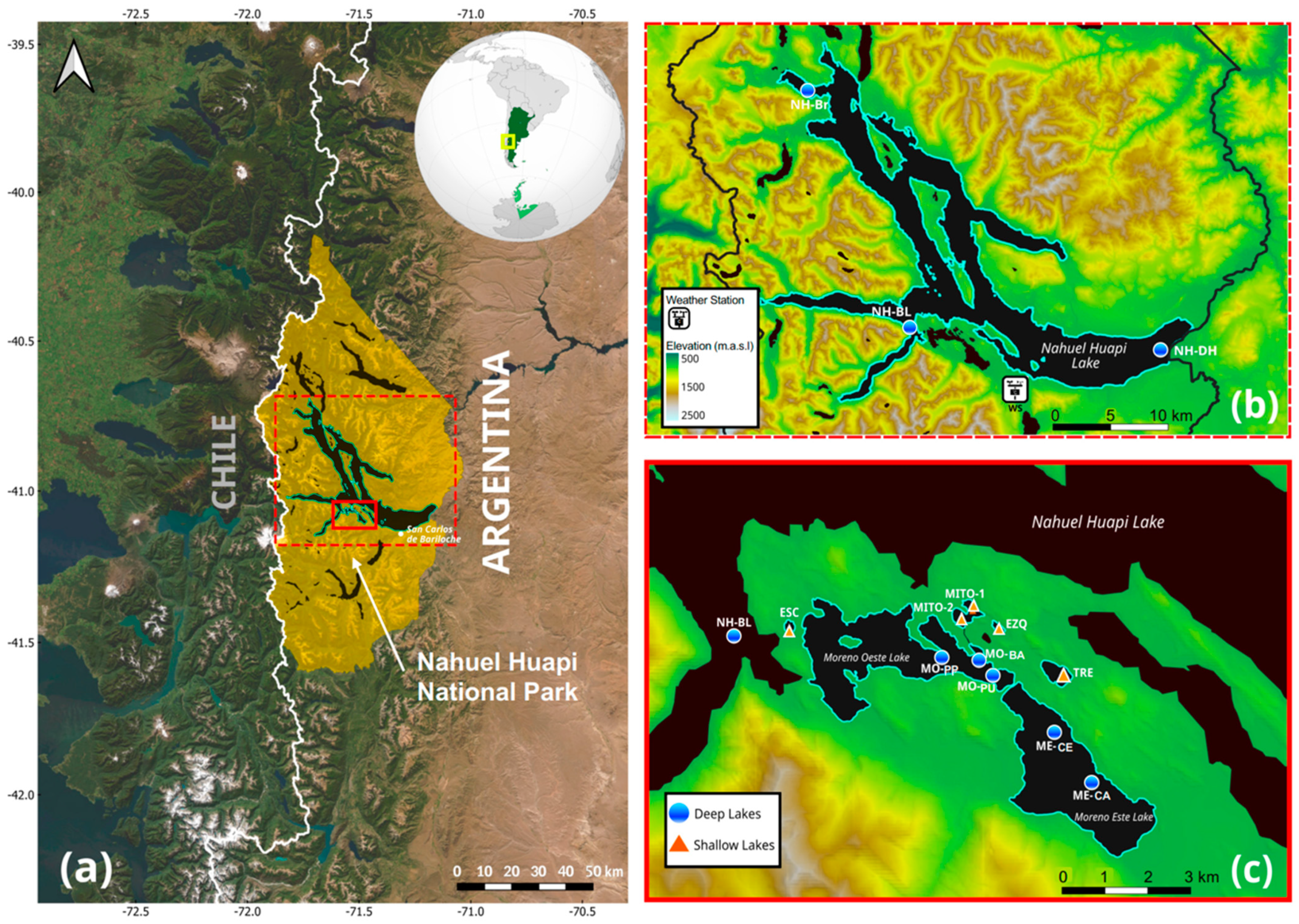
2.1. Study Area, Lakes, and Region Characteristics

This study focused on seven piedmont lakes (768–785 m.a.s.l.) within the Lake Nahuel Huapi basin located in North Andean Patagonia, Argentina (40.145–41.592S; 71.028–71.966W) (Figure 1). The region belongs to the Glacial Lakes District of the Southern Andes, being the largest lacustrine district of Argentina [44]. The Nahuel Huapi National Park features an extensive hydrographic system characterized by a large landscape heterogeneity that includes large, deep mountain lakes (area > 5 km²; Z_MAX > 90 m) with a warm monomictic thermal regime as well as small, shallow polymictic lakes (area < 1 km²; Z_MAX < 20 m) that can freeze during severe winters. North Andean Patagonian lakes and streams are oligotrophic or ultra-oligotrophic and rank among the world’s most unproductive systems. They are characterized by limiting nutrient levels [45,46], very low chlorophyll a concentration [47,48], very low to moderate DOC concentrations [42,43], and elevated water transparency [49,50].

The North Andean sector of Patagonia experiences a transitional oceanic-continental cold temperate climate with dry summers dominated by prevailing westerly winds from the South Pacific subtropical anticyclone. The precipitation regime in the region is highly seasonal due to the southward movement of the anticyclone in summer and its opposite movement in winter [51]. This seasonal climate creates two contrasting scenarios, the dry season (from October to April) that coincides with the peak of solar radiation and moderate to high air temperatures and the wet season (from the end of March to September) that aligns with the cold period and accounts for 73% of the annual precipitation with a mean value of ~1800 mm year⁻¹ [52,53]. The study lakes are primarily surrounded by temperate evergreen forests, featuring mixed forests of Nothofagus dombeyi (Mirb.) Blume and Austrocedrus chilensis (D.Don) Florin et Boutleje.

2.2. Water Collection and Processing

In this work, we pooled data collected during different campaigns carried out from 2013 to 2021 in seven North Andean Patagonian lakes (13 sampling sites, Figure 1). The study included three deep lakes, Lake Nahuel Huapi (NH), Lake Moreno Oeste (MO), and Lake Moreno Este (ME), and four shallow lakes, Lake Trébol (TRE), Lake Escondido (ESC), Lake Morenito (MITO), and Lake Ezquerra (EZQ) (Figure 1,

Table 1. Descriptive statistics of the in situ CDOM absorption coefficients at 440 nm [$a_{cdom}^{440}$] and main characteristics of the seven study lakes.

Lakes		Geographic Location	ZMAX [m]	${\mathit{a}}_{\mathit{c}\mathit{d}\mathit{o}\mathit{m}}^{\mathbf{440}}$ [m−1]			N
				Average ± 1SD	Min	Max
Lake Ezquerra	EZQ	41°03′S; 71°30′W	3.6	1.83 ± 0.17	1.52	2.08	9
Lake Escondido	ESC	41°03′S; 71°34′W	8.0	1.05 ± 0.41	0.61	1.79	11
Lake Morenito	MITO	41°03′S; 71°31′W	12.0	0.47 ± 0.12	0.34	0.75	23
Lake Trébol	TRE	41°04′S; 71°29′W	12.0	0.30 ± 0.05	0.20	0.35	8
Lake Moreno Oeste	MO	41°04′S; 71°31′W	90.0	0.063 ± 0.018	0.033	0.098	27
Lake Moreno Este	ME	41°05′S; 71°29′W	106.0	0.053 ± 0.019	0.027	0.095	21
Lake Nahuel Huapi	NH	41°02′S; 71°27′W	454.0	0.060 ± 0.034	0.033	0.106	8

). Sampling sites were geographically recorded with GPS and revisited during different campaigns. Water samples were carried out during both the dry and wet seasons to include the previously reported natural spatio-temporal variability of DOM in the North Andean Patagonian lakes [42,54,55,56]. Surface discrete water samples (at 0.5–5 m depth) were collected from a boat with a Kemmerer bottle (4.2 L) at deep, offshore points of each lake. Samples were poured into acid-cleaned polycarbonate carboys and stored in darkness. Overall, 107 water samples were obtained during the complete study period (Table 1).

Within 5 h from sampling, water samples were filtered in the laboratory through prerinsed 0.22 μm PVDF membranes (Millipore) to assess DOM characterization through absorbance spectroscopy. Absorbance of CDOM was determined from the filtered samples with a dual beam spectrophotometer (Shimadzu UV-1800) using 10 cm quartz cuvettes. Absorbance spectra were recorded between 200 and 800 nm at 1 nm intervals against a blank of ultrapure grade water (Milli-Q). The average absorbance from 700 to 800 nm was subtracted from each spectrum to correct for offsets due to several instrument baseline effects [57,58]. Absorbance units were converted to absorption coefficients (a_λ in units m⁻¹) as an indicator of CDOM quantity following [16]:

a_λ = 2.303·A_λ/l

(1)

where a_λ (m⁻¹) is the Napierian CDOM absorption coefficient at wavelength _λ (nm), A_λ is the spectrophotometric measured absorbance of the filtered lake water sample (dimensionless), and l is the optical pathway of the quartz cuvette in metres [59]. CDOM absorption was characterized by absorption coefficients at the reference wavelength of 440 nm ($a_{cdom}^{440}$, m⁻¹), a value commonly used in limnological studies.

Furthermore, on several occasions, particulate absorption was also quantified to characterize the absorption budget of the study lakes. Water samples (1–2 L) were filtered using 25 mm diameter GF/F filters. After filtration, absorbance scans of total particulate matter were measured by a dual beam spectrophotometer (Shimadzu UV-1800) from 300 to 750 nm at 1 nm intervals against a blank clean filter wetted with Milli-Q water using the quantitative filter technique (QFT) and the simple transmittance method (T-Mode). The QFT method was applied according to NASA protocols for absorption coefficient measurements [59]. Absorption coefficients of non-algal particles were determined with the methanol extraction method [60]. Absorption coefficients of total particulate matter $a_p^{\lambda }$ (first measurement) and absorption by non-algal particles $a_{nap}^{\lambda }$ (measurement after extraction) were estimated according to the equation:

$$a_p^{\lambda },a_{nap}^{\lambda }={\displaystyle \frac{2.303 ·{Af}_{\lambda } ·S}{V·{\beta }_{\lambda }}}$$

(2)

where Af_λ is the measured absorbance with QFT (before and after methanol pigments extraction), S is the clearance area of the filter, V is the volume of filtered water, and β_λ is the amplification factor vector [61]. The β_λ factor was calculated following [62]. Phytoplankton absorption was determined as $a_p^{\lambda }$ − $a_{nap}^{\lambda },$and the tabulated absorption coefficient for pure water was taken from [63].

2.3. Satellite Imagery Processing

In this study, the satellite Landsat 8-OLI was used for retrieving the CDOM absorption coefficient. Landsat Collection 2, Level 1 terrain-corrected (L1TP), and Level 2 surface reflectance (L2SP) imageries at path/row (232/088) were freely downloaded from the USGS website (https://earthexplorer.usgs.gov/) (accessed on 17 February 2022). Landsat 8-OLI is a multispectral sensor that take measurements in the visible, near infrared, and shortwave infrared portions of the electromagnetic spectrum with a 30 m spatial resolution and a return interval of 16 days. Considering that lacustrine CDOM concentration has been shown to be stable on a short-term basis (days to weeks), Landsat imagery within 30 days of field sample collection was used for calibration/validation modelling. This time window is within the previously reported interval used by several authors in CDOM remote sensing of inland waters [24,32,37,38,39]. On average, field samples were collected within 9 days of satellites overpass, ranging from the same day to 26 days (the latter only on two occasions). The Landsat L1TP images were evaluated as top-of-atmosphere (TOA) and bottom-of-atmosphere (BOA) reflectance. Atmospherically uncorrected images were evaluated using calibration/validation models since several authors have found good results using TOA for monitoring of water quality [36,64]. Images were converted from digital number to TOA reflectance using the band-specific rescaling factors provided in the metadata files associated with each image. See the method described in Chapter 4 of Landsat 8 Science data user handbook (https://www.usgs.gov/media/files/landsat-8-data-users-handbook) (accessed on 17 February 2022).

To get BOA reflectance images, four different atmospheric correction algorithms were assessed: Dark Object Subtraction (DOS1), Quick Atmospheric Correction (QUAC), and the iterative two-band bio-optical-based algorithm (L2gen). Additionally, L2SP surface reflectance images (processed with the Land Surface Reflectance Code, LaSRC) are ready-made standard Landsat 8 products from the NASA Goddard Flight Center for terrestrial applications. In brief, the DOS method is based on image information and considers only the correction of atmospheric additive scattering [65]. The main idea is to identify the darkest pixel in a spectral band in TOA reflectance and subtract this value from every pixel within the respective band. This procedure was performed using the Semi-automatic Classification Plugin (SCP) [66] in the open-source GIS software QGIS 3.28 Firenze [67]. QUAC is also an in-scene technique and performs the variance equalization of an image based on selected endmembers that can be characterized by a unique spectrum from an available library collection [68]. QUAC requires only the radiometric calibration and centre wavelength information of each band from the multispectral sensor. This procedure was applied to the Landsat 8 images using the ENVI 5.3 imaging processing software package. In contrast, L2gen 9.6.0 V2023.1 (Level 2 Generator) is a software tool developed by NASA, which is primarily used for processing ocean colour satellite data. However, it has also been adapted for atmospheric correction of Landsat images. The tool is part of the SeaDAS (SeaWiFS Data Analysis System) freely available software suite. L2gen employs a combination of radiative transfer models to simulate the interaction of light with the atmosphere. It accounts for scattering and absorption by gases, aerosols, and clouds and is used to produce remote sensing reflectance products for Landsat 8 [69]. The four atmospheric corrections described above have been successfully used either for estimating the in situ remote sensing reflectance or for remote monitoring of water quality properties in inland and coastal waters [70,71,72,73,74].

Finally, from TOA and BOA reflectance images, a 3 × 3 pixel window was defined as the water area of interest at each lake sampling point and used to extract average reflectance from visible and near-infrared bands. Only nearly cloud-free scenes were used in the calibration/validation process. Furthermore, a visual inspection of the obtained multi-spectral reflectance images was used to remove scenes with anomalous spectra, generally associated with strong wind days, high-altitude cloud contamination, and, particularly for shallow lakes, the presence of ice or macrophytes. The abundant cloudiness of the study area and the time window selected between satellite visit date and sampling yielded 64 calibration measurements corresponding to 20 clear image paths of Landsat 8 from September 2013 to October 2021.

2.4. Model Calibration

Given the lack of in situ radiometric measurements, Landsat 8 TOA or BOA reflectance obtained using different atmospheric corrections was used to develop a model to retrieve $a_{cdom}^{440}$. The potential of all visible bands [B1 (deep blue), B2 (blue), B3 (green), and B4 (red)] and near-infrared band (B5, NIR) of the Operational Land Imager (OLI) instrument in Landsat 8 was explored as well as all possible band ratios to predict CDOM. To create an empirically based algorithm using satellite imagery, forward stepwise regressions were performed. The CDOM absorption coefficient ($a_{cdom}^{440}),$as well as its log-transformed value (${Ln a}_{cdom}^{440})$, were the dependent variables, and single bands and all band ratio permutations (in their original and log-transformed forms) were the independent variables. From the forward stepwise results, the two independent variables that contributed most to the regression fit were selected and applied in a multiple linear regression procedure (MLR) following the general form:

$$a_{cdom}^{440} or Ln \left(a_{cdom}^{440}\right)=b1·(band or band\text{-}ratio)+b2·(band or band\text{-}ratio)+b3$$

(3)

where $a_{cdom}^{440}$ or ln ($a_{cdom}^{440}$) are the CDOM absorption coefficient at 440 nm (in its untransformed and log-transformed forms), b1–b3 are the regression coefficients of calibration data, and band or band ratio combination is derived from the average reflectance obtained for each evaluated 3 × 3 pixel window. The forward stepwise regression and multiple linear regression steps were repeated for each of the five evaluated datasets (TOA, DOS1, QUAC, L2gen, and LaSRC). In all the regression procedures, data were tested to verify normality (Shapiro–Wilk test) and homoscedasticity (Spearman’s rank correlation). In multiple linear regressions, to prevent collinearity between the two evaluated independent terms, the variable inflation factor (VIF) was calculated, and only models with VIF < 3 were selected [75]. In our dataset, the log-transformed value of $a_{cdom}^{440}$ presented better correlation with both Landsat bands and band ratios than the untransformed absorption coefficient; therefore, MLRs were performed with ln $a_{cdom}^{440}$ as the dependent variable.

2.5. Model Validation

The best fitting model obtained for each TOA and BOA reflectance product was validated using the leave-one-out cross-validation (LOOCV) technique. This method, proposed by [76], is a rigorous cross-validation method that is considered an unbiased estimator of model validation [77], being a valuable tool to validate algorithms in studies with limited data, such as this study. To validate the best fitting model, one sample was excluded as a validation datum, while the remaining 63 samples were used as training data to fit a regression model with the same form as the best fitting model using the least-squares technique. The resulting regression model was then used to estimate the ln $a_{cdom}^{440}$ value for the excluded sample. This process was repeated 64 times to estimate the CDOM values of each water sample with extracted remote sensed information. The calibrated models’ performance was evaluated using four statistical indicators. The coefficient of determination (R²), the root mean square error (RMSE), the mean absolute percentage error (MAPE), and the systematic error (bias). For better interpretability, measured and estimated CDOM values were converted back from the natural logarithmic scale before computing the evaluation metrics. With a resulting unit of m⁻¹, these metrics were defined as:

$$RMSE=\sqrt{{\displaystyle \frac{\sum _{i=1}^N{\left(x_i-y_i\right)}^2}{N}}}$$

(4)

$$MAPE=100.{\displaystyle \frac{1}{N}}\sum _{i=1}^N{\displaystyle \frac{\left|x_i-y_i\right|}{y_i}}$$

(5)

$$Bias=\sum _{i=1}^N{\displaystyle \frac{\left(x_i-y_i\right)}{N}}$$

(6)

where x_i and y_i represent the satellite-estimated and the in situ observed value of the parameter of interest (i.e, $a_{cdom}^{440}$ values), respectively. N is the number of samples in the dataset.

2.6. CDOM Time Series

To evaluate spatio-temporal variability of the CDOM absorption coefficient in the study lakes, all available images of Landsat 8 (Collection 2, Level 1 terrain-corrected, and Level 2 surface reflectance) were freely obtained from the USGS website. Images covering the area of interest were downloaded from January 2016 to December 2020 (a total of 40 images were selected). The best performing band and band ratio empirical model obtained was used to atmospherically correct the images and retrieve ln $a_{cdom}^{440}$ values. Then, a cloud-free 3 × 3 pixel window at each lake was extracted from images and used for time series analyses following the same methodology described in Section 2.3. Satellite-estimated ln $a_{cdom}^{440}$values were converted from multiplicative (logarithmic) to linear space (i.e., obtaining a satellite-derived $a_{cdom}^{440}$value). On the other hand, monthly mean climatological $a_{cdom}^{440}$maps were also calculated for the study lakes from the five-year study period. Lake polygons were downloaded from the Instituto Geográfico Nacional (IGN) [78] and used to extract satellite-derived $a_{cdom}^{440}$values for each entire lake. Only images with less than 10% cloud cover over each lake studied were considered for mapping.

2.7. Meteorological Variables and Lake Hydrogeomorphic and Watershed Characteristics

A suite of environmental variables was evaluated to investigate the factors influencing CDOM dynamics in North Andean Patagonian lakes. These included meteorological time series data and lake hydrogeomorphic and watershed characteristics. Air temperature (°C), rain precipitation (mm), wind speed (km h⁻¹), solar radiation (W m²), and UV index (dimensionless) were collected daily for the five-year study period from a meteorological monitoring station (Davis Ventage Pro^®) located at GESAP laboratory (INIBIOMA, Bariloche, Argentina) (Figure 1a). The meteorological records from this station reliably characterize the general meteorological conditions of the study area, with most of the sampling sites located within a 15 km radius, with the exception of the NH-BR and NH-DH sites, which were located at the northwestern and northeastern ends of Lake NH, respectively (Figure 1b). Meteorological variables were assessed as monthly mean values for each of the 5 study years, except for rain precipitation. Previous studies have indicated that cumulative rainfall is a key variable in explaining the seasonality of CDOM in Patagonian lakes [55,56,79]. Consequently, we analyzed the rain precipitation as an accumulative monthly value during the five-year study period and at different time windows (7, 14, 21, 30, 60, 90 days) prior to the satellite visit over target lakes.

Regarding the lakes’ hydrogeomorphic and watershed characteristics, data for each of the seven studied lakes were either obtained from previous works [56,78,79,80,81,82,83,84,85,86], or from HydroLAKES v. 1.0 [87] when lake parameters were not covered by earlier local studies. The HydroLAKES is a global database that includes all lakes and reservoirs with a surface area > 0.1 km² and contains an important information about different water and catchment characteristics. The following lake and watershed characteristics were evaluated: lake area (Km²), lake perimeter (Km), lake volume (Km³), lake perimeter to lake area ratio (lake peri./lake area, Km⁻¹), lake depth maxima (Z_MAX, m), lake depth average (Z_AVG, m), water resident time (WRT, years), watershed area (Km²), and watershed area to lake volume ratio (wshd. area/lake volume, Km⁻¹). These features were evaluated for each of the seven study lakes as static variables, and therefore, seasonal changes were not considered. In contrast, the water storage of Lake Nahuel Huapi (hm³) was obtained as monthly records from published hydrometeorological reports by the Autoridad Interjurisdiccional de Cuencas (AIC) [88]. North Andean Patagonian lakes have shown a clear synchrony of water levels between dry and wet periods [79], and the water storage of Lake Nahuel Huapi has been previously considered as a good proxy of water level at the basin scale [56].

Overall, a total of 21 environmental variables were evaluated to explain the spatio-temporal variability of the satellite-derived $a_{cdom}^{440}$ values throughout the five-year study period (see Table S1 for a statistical description of the evaluated environmental variables).

2.8. Gradient Boosting Regression

Gradient boosting regression tree (GBRT) is a highly prevalent machine learning algorithm that has demonstrated efficacy across a multitude of domains, including ecology and environmental studies [89,90,91]. GBRT employs the strengths of two powerful algorithms: regression trees, which model the relationship between a response variable and its predictors through recursive binary splits, and boosting, an adaptive technique that enhances predictive performance by combining numerous simple models. GBRT enables the analysis of the relative importance of different types of explanatory variables as well as the investigation of the manner in which distinct parameters influence the prediction of a response variable. This approach has the potential to elucidate underlying environmental processes [92,93]. GBRT offers significant improvements because it does not require the prior transformation or elimination of outliers, which results in enhanced performance across a wide range of tasks. One of the primary strengths of GBRT is its ability to model complex interactions and non-linearities, which makes it less sensitive to the problems caused by collinear features [94]. In this work, GBRT was implemented to investigate the relationship between satellite-derived${ a}_{cdom}^{440}$ values (in a linear space) and the 21 environmental variables assessed (meteorological, lake hydrogeomorphic, and watershed characteristics). Satellite-derived mean${ a}_{cdom}^{440}$ values obtained from each of the 3 × 3 pixel windows at each lake for the five-year study period were used as dependent variables. On the other hand, environmental variables were implemented as independent, explanatory variables. Although collinearity is not a critical issue in GBRT, it is beneficial to address it to achieve more interpretable results. In order to reduce the number of explanatory variables in the final GBRT setup, all the environmental variables were cross-correlated using the corrplot package in R software 4.4.1. If several variables exhibited a significant correlation with one another (R > 0.5), the variable exhibiting the highest correlation with satellite-derived${ a}_{cdom}^{440}$ was retained. To validate the GBRT model, the dataset was randomly divided into training (70%) and testing subgroups (30%). Furthermore, a k-fold cross-validation (k = 10) was performed on the training dataset, providing a more reliable estimate of model performance. The resulting model was then subjected to evaluation using the test dataset.

2.9. Statistical Processing

For analyzing differences in mean values of the CDOM absorption coefficient (in situ and satellite-derived) among lakes, seasons, and months, a one-way ANOVA test followed by the Holm–Sidak pairwise comparisons method was used to determine significance. When the normality test failed (Shapiro–Wilk), the non-parametric Kruskal–Wallis test was applied followed by Dunn’s method for all pairwise comparisons. Multiple linear regressions (MLRs) were performed in R free software, version 4.3.1 [95]. For stepwise (backward direction), the step function was implemented, and the degree of multicollinearity was evaluated to determine the variance inflation factor (VIF) using the car package and the vif function. Validation of empirical band and band ratio models were performed using the LOOCV method in R software using base code and the TrainControl function from the caret library. Gradient boosting regression tree (GBRT) was implemented in R using the gbm package.

3. Results

3.1. In Situ CDOM Absorption and Water Quality Measurements

Sampled surface waters of the study lakes presented very low to moderate values of CDOM, with absorption coefficients at 440 nm ranging widely from 0.012 to 2.12 m⁻¹ (mean $a_{cdom}^{440}$ = 0.41 ± 0.54 m⁻¹). Deep lakes presented significantly lower mean CDOM values ($a_{cdom}^{440}$ = 0.06 ± 0.02 m⁻¹) than shallow lakes ($a_{cdom}^{440}$ = 0.80 ± 0.58 m⁻¹) (KW-ANOVA, p < 0.001). The lowest mean $a_{cdom}^{440}$ value was registered in ME (0.053 ± 0.019 m⁻¹) and highest value in EZQ (mean $a_{cdom}^{440}$ = 1.83 ± 0.17 m⁻¹). Further information of in situ CDOM values and main lake properties are shown in Table 1.

Even if an uneven distribution of water samples through years and month was obtained, a clear seasonality in in situ $a_{cdom}^{440}$ values could be elucidated irrespective of the lake’s type. Overall, shallow lakes presented with around 39% lower mean $a_{cdom}^{440}$ values (0.42 ± 0.13 m⁻¹) during the austral summer and early autumn period than during the late winter and spring period (0.69 ± 0.43 m⁻¹). Deep lakes also showed lower mean CDOM values (around 23%) during the summer and early autumn period ($a_{cdom}^{440}$ = 0.052 ± 0.017 m⁻¹) than the winter and spring period ($a_{cdom}^{440}$ = 0.063 ± 0.021 m⁻¹).

Regarding the underwater light climate in the study lakes, the total absorption budget showed the importance of CDOM in the light absorption process at lower wavelengths (Figure S1). CDOM dominated the total absorption coefficient between 380 and ~510 nm in deep lakes (e.g., ME, Figure S1a) and up to ~580 nm in shallow lakes (e.g., ESC, Figure S1b), except for TRE. In this lake, the total absorption in the blue and green wavelengths was co-dominated by both CDOM and suspended particles (mainly non-algae and detritus) (Figure S1c). In all lakes, irradiances > 600 nm were mainly absorbed by the water molecules themselves.

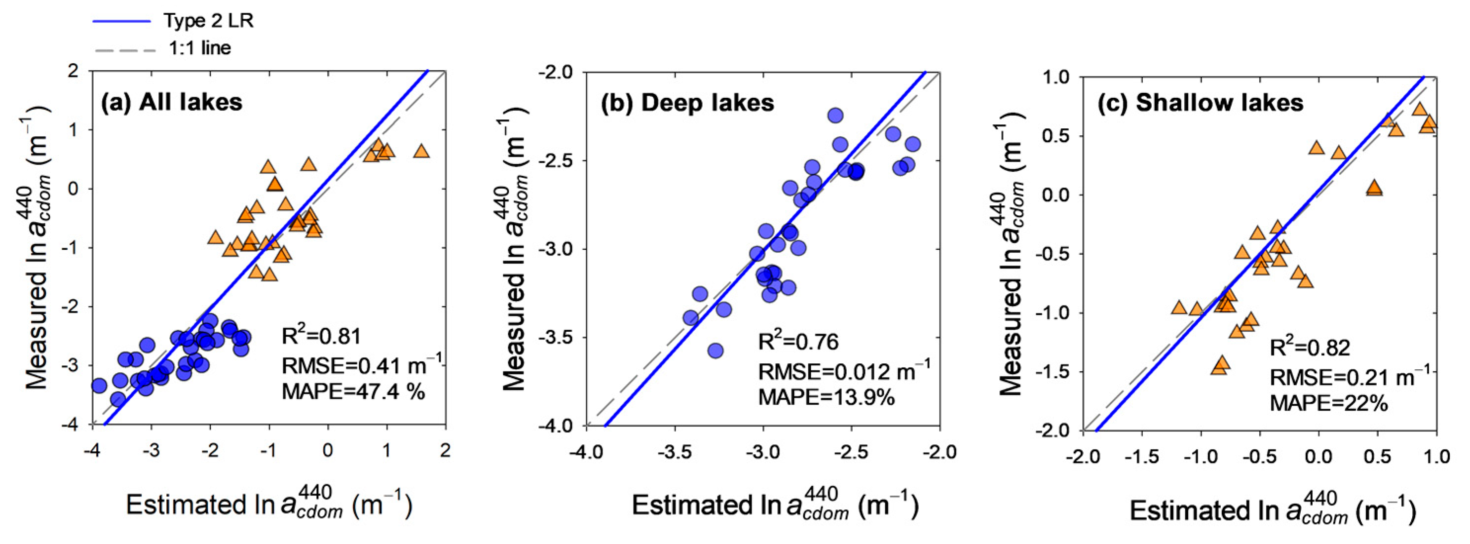
3.2. CDOM Absorption Retrieval Algorithms

Table 2. Coefficients and goodness of fit parameters from multiple linear regression-based algorithms for retrieving ln $a_{cdom}^{440}$values from calibration datasets with different atmospheric correction routines and data groups evaluated.

Data Levels	Independent Variables [x1, x2] #	Equation Coefficients			R2	RMSE [m−1]	p Value
		$\mathbf{ln} {\mathit{a}}_{\mathit{c}\mathit{d}\mathit{o}\mathit{m}}^{\mathbf{440}}$ = b0 + b1.x1 +b2.x2
		b0	b1	b2
All lakes [N = 63]
TOA	B3/B4, B1/B2	−35.62	−11.03	40.60	0.79	0.34	<0.001
DOS 1	B2/B4, B3/B1	10.67	−6.35	−3.74	0.84	0.40	<0.001
QUAC	Ln (B2/B4), Ln (B1/B2)	0.63	−2.80	3.96	0.83	0.36	<0.001
L2gen	B2/B4, B1/B2	−3.11	−1.71	5.40	0.74	0.38	<0.001
Deep lakes [N = 32]
TOA	B3/B4	5.03	−4.30		0.57	0.012	<0.001
DOS 1	B2/B4, B2	−0.823	−2.57	104.72	0.67	0.012	<0.001
QUAC	B2/B4, B2/B5	−1.67	−0.18	−0.18	0.81	0.010	<0.001
L2gen	B4	−3.53	97.36		0.43	0.014	<0.001
Shallow lakes [N = 32]
TOA	B4/B3, B1/B2	−46.86	20.12	26.17	0.83	0.23	<0.001
DOS 1	Ln (B3/B4), Ln B5	2.77	−4.96	0.61	0.82	0.24	<0.001
QUAC	Ln (B3/B4), Ln (B4/B5)	0.15	−1.8	−0.48	0.85	0.22	<0.001
L2gen	B4/B3, B2/B4	−7.63	8.91	0.88	0.76	0.26	<0.001

# are the bands and/or band combinations [in normal or logarithmic form] used as independent variables in two-term multiple linear regression models.

shows the calibration results of retrieving ln $a_{cdom}^{440}$ with different satellite data levels (i.e., TOA, DOS1, QUAC, and L2Gen). The standard USGS land surface reflectance product (LaSRC) rendered unreal results (Rs values < 0) for B4 and B5 bands in a high proportion of target pixels in the study scenes, and consequently were not taken into account in the model calibration/validation process. MLR models were run with the entire dataset (general model) as well as shallow and deep lakes separately (lake type-specific models) (Table 2).

Considering the entire dataset, the calibration results showed a good performance with DOS1 and QUAC routines presenting higher determination coefficients (R² = 0.84 and 0.83, respectively) than the other two evaluated routines (Table 2). These two models used the band ratio B2/B4 (blue/red) or ln (B2/B4) as one of the model terms. A validation step using the LOOCV method corroborated these results, with QUAC atmospheric correction showing the best performance for the entire dataset (R² = 0.81, RMSE = 0.41 m⁻¹, and MAPE = 47.4%) (

Table 3. LOOCV validation results and assessment of model performance for different atmospheric correction routines and data groups. The best results in the analysis of model performance for retrieving ln $a_{cdom}^{440}$values are shown in bold.

Data Levels	R2	RMSE [m−1]	MAPE [m−1]	Bias [m−1]	Slope
All lakes [N = 64]
TOA	0.77	0.39	61.8	−0.003	1.11
DOS 1	0.79	0.59	47.6	0.005	1.10
QUAC	0.81	0.41	47.4	−0.005	1.09
L2gen	0.71	0.39	63.8	−0.106	1.15
Deep lakes [N = 32]
TOA	0.51	0.013	19.5	−0.0011	1.29
DOS 1	0.57	0.014	17.9	−0.0008	1.19
QUAC	0.76	0.012	13.9	−0.0006	1.10
L2gen	0.36	0.015	24.3	−0.0016	1.51
Shallow lakes [N = 32]
TOA	0.80	0.27	23.0	−0.005	1.07
DOS 1	0.78	0.32	25.5	−0.004	1.07
QUAC	0.82	0.21	22.0	−0.018	1.08
L2gen	0.71	0.29	25.5	−0.055	1.15

, Figure 2a). This general model, however, presented a poor predictive performance for $a_{cdom}^{440}$ values < 0.11 m⁻¹ (typical values fond in the analyzed deep lakes), with a clear overestimation for values between 0.05 and 0.11 m⁻¹ and an underestimation for values < 0.05 m⁻¹. Better results were obtained when the models were calibrated for deep and shallow lakes separately. Calibrated results for deep lakes showed that QUAC and DOS1 outperformed TOA and L2Gen (Table 2). QUAC showed the best results with a model using B2/B4 (blue/red) and B2/B5 (blue/NIR) band ratios (R² = 0.81, RSME = 0.010) (Table 2). In this model, the band ratio B2/B4 explained, by itself, the highest proportion of observed variation in ln $a_{cdom}^{440}$ (R² = 0.72) (Table S2).

Validated models showed QUAC routine to render the more accurate performance for deep, low-coloured lakes (R² = 0.76, RMSE = 0.012 m⁻¹ and MAPE = 13.9% m⁻¹) (Table 3, Figure 2b). Regarding shallow lakes, the lake type-specific model showed better results with QUAC and TOA routines. A slightly better fit was observed with QUAC that included the ln (B3/B4) (green/red) and ln (B4/B5) (red/NIR) band ratios (R² = 0.85, RMSE = 0.22) (Table 2).

The single band ratio ln (B3/B4) explained much of the observed variation in ln $a_{cdom}^{440}$ (R² = 0.78) (Table S2). The validation procedure showed that the QUAC model rendered the best performance for retrieving ln $a_{cdom}^{440}$ in shallow lakes (R² = 0.82, RMSE = 0.21 m⁻¹, and MAPE = 22%), closely followed by the model using TOA reflectance (Table 3, Figure 2c).

We compared our results with two previously published models for estimating CDOM in inland waters, both using BOA reflectance from the QUAC routine. Kutser and coauthors [39] found good results with a power model using the green/red band ratio. Similarly, Alcântara and coauthors [96] achieved accurate estimations using a second-degree polynomial function with a red/blue band combination. In general, these two models showed lower predictive performance with our in situ data compared to the best models presented here (Figure S3, Table 2). Calibration results for the entire dataset showed that both models (power and polynomial) presented relatively high errors (RMSE > 0.29) and low coefficients of determination (R² < 0.72). Both models notably overestimated the low CDOM values observed in deep lakes (Figure S3a,d). However, when deep and shallow lakes were considered separately, the power model showed slightly lower performance for shallow lakes (RMSE = 0.25 and R² = 0.79) compared to our specific model (Figure S3c, Table 2). Similarly, the polynomial model yielded comparable calibration results for deep lakes (RMSE = 0.013 and R² = 0.75) when contrasted with our best model (Figure S3e, Table 2).

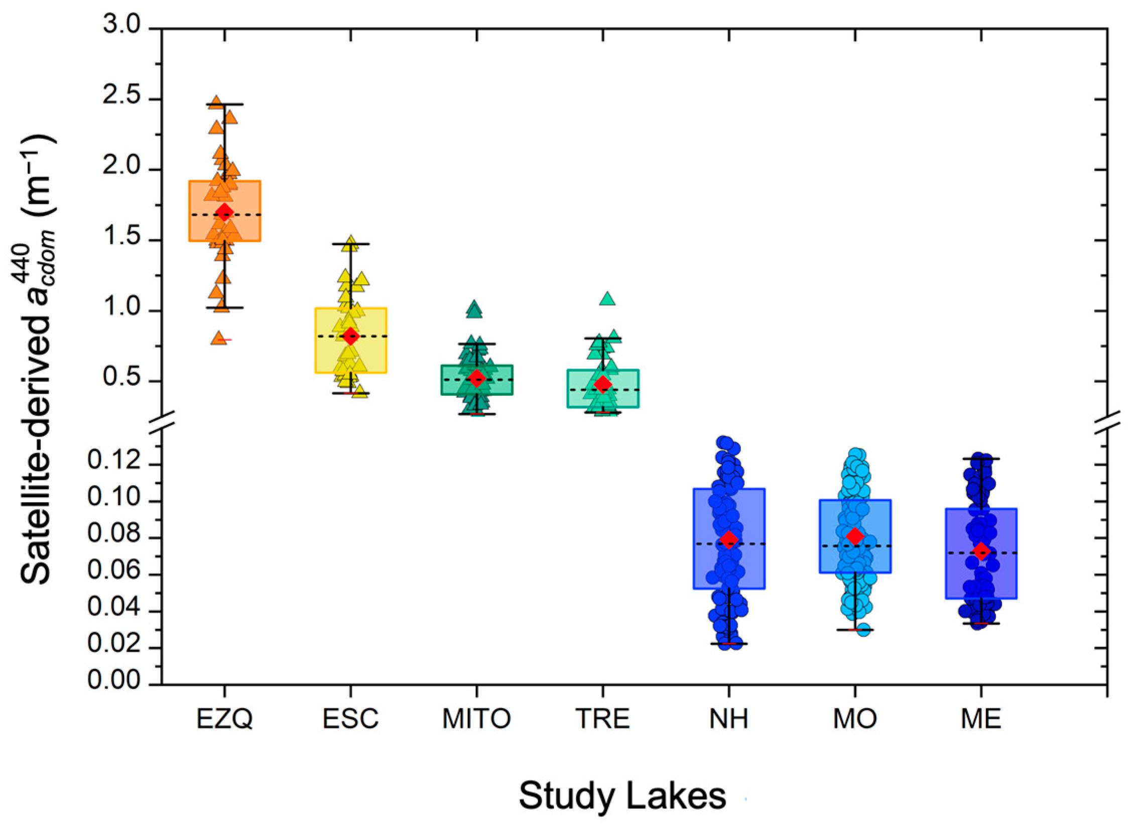
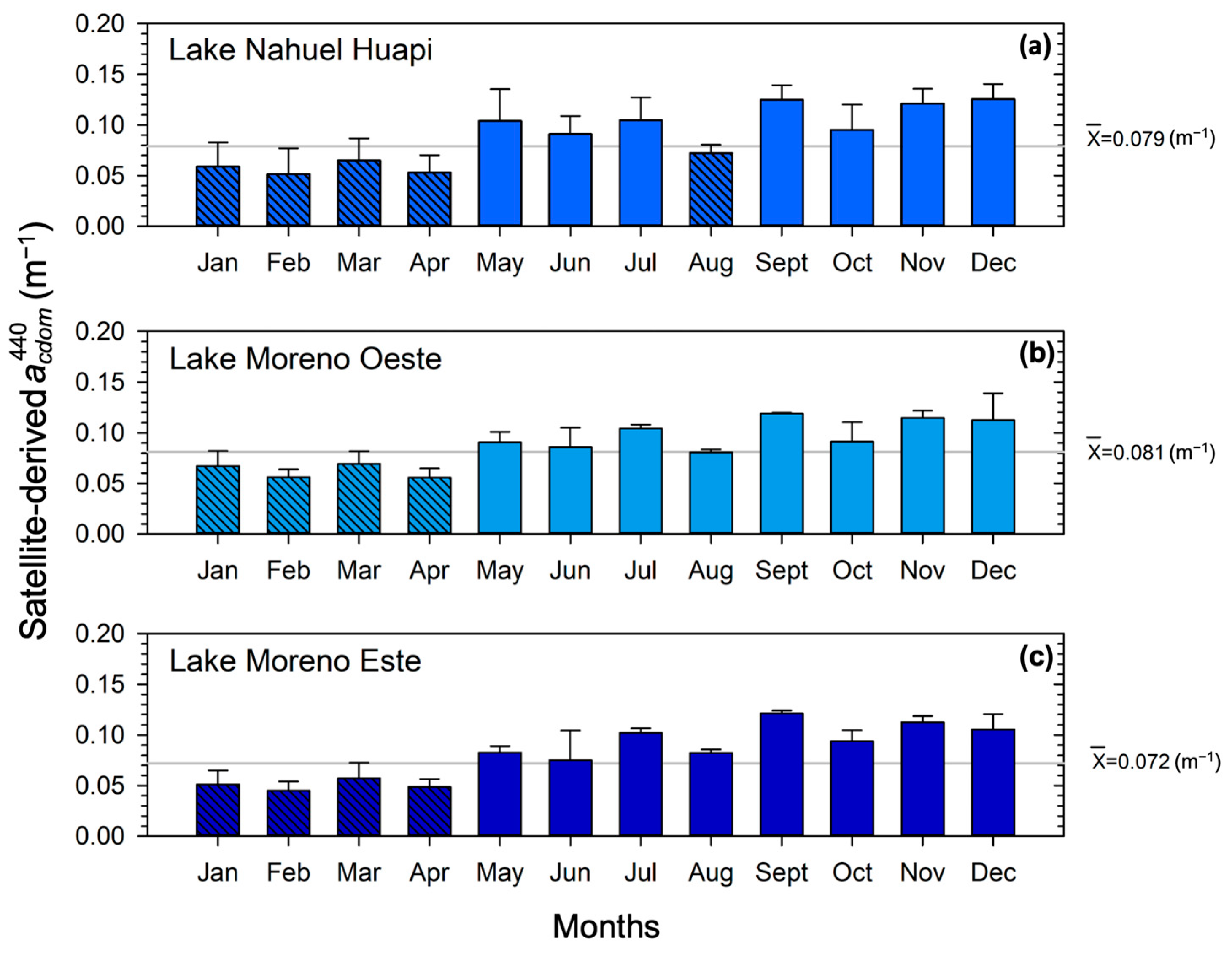
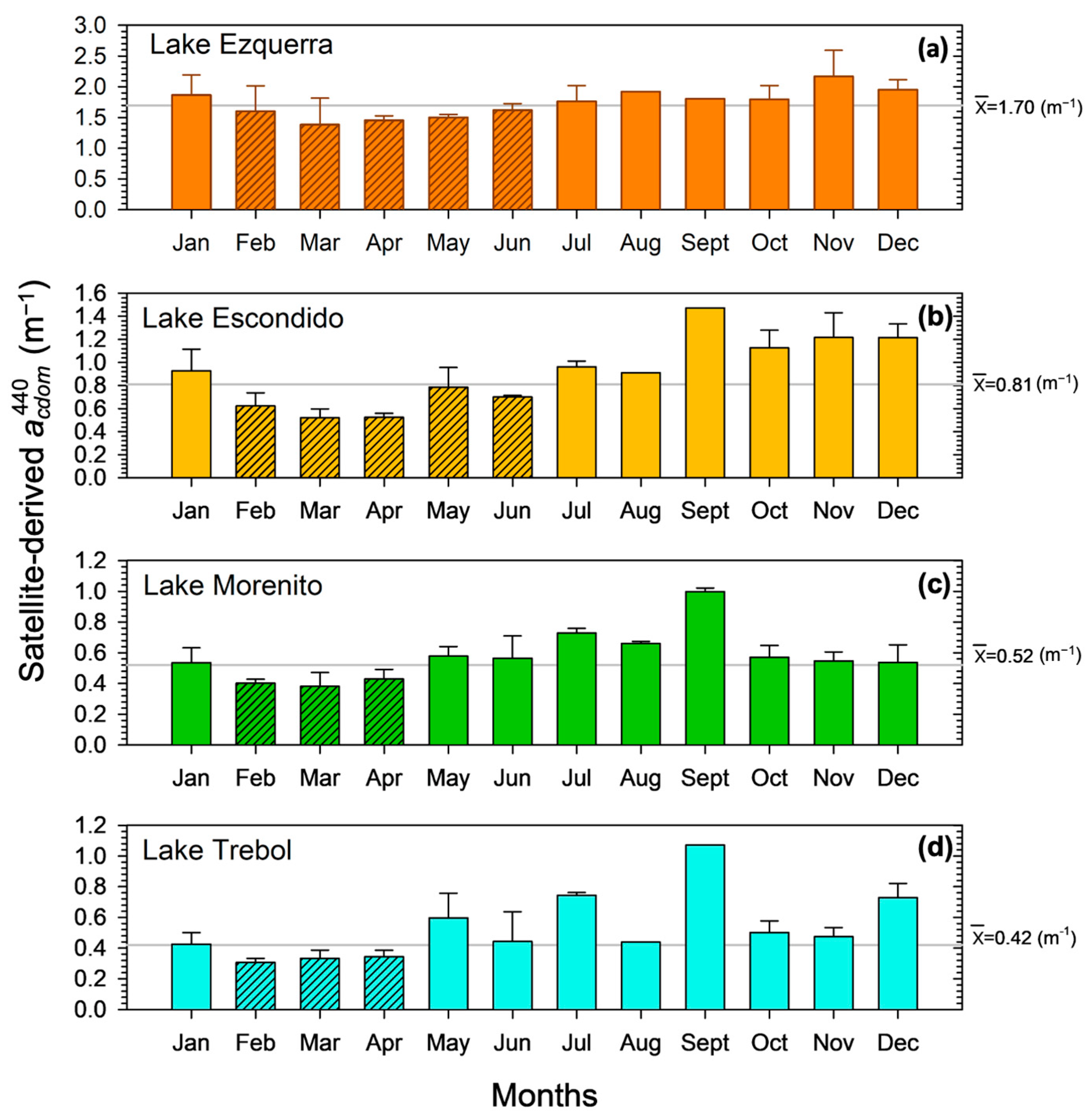
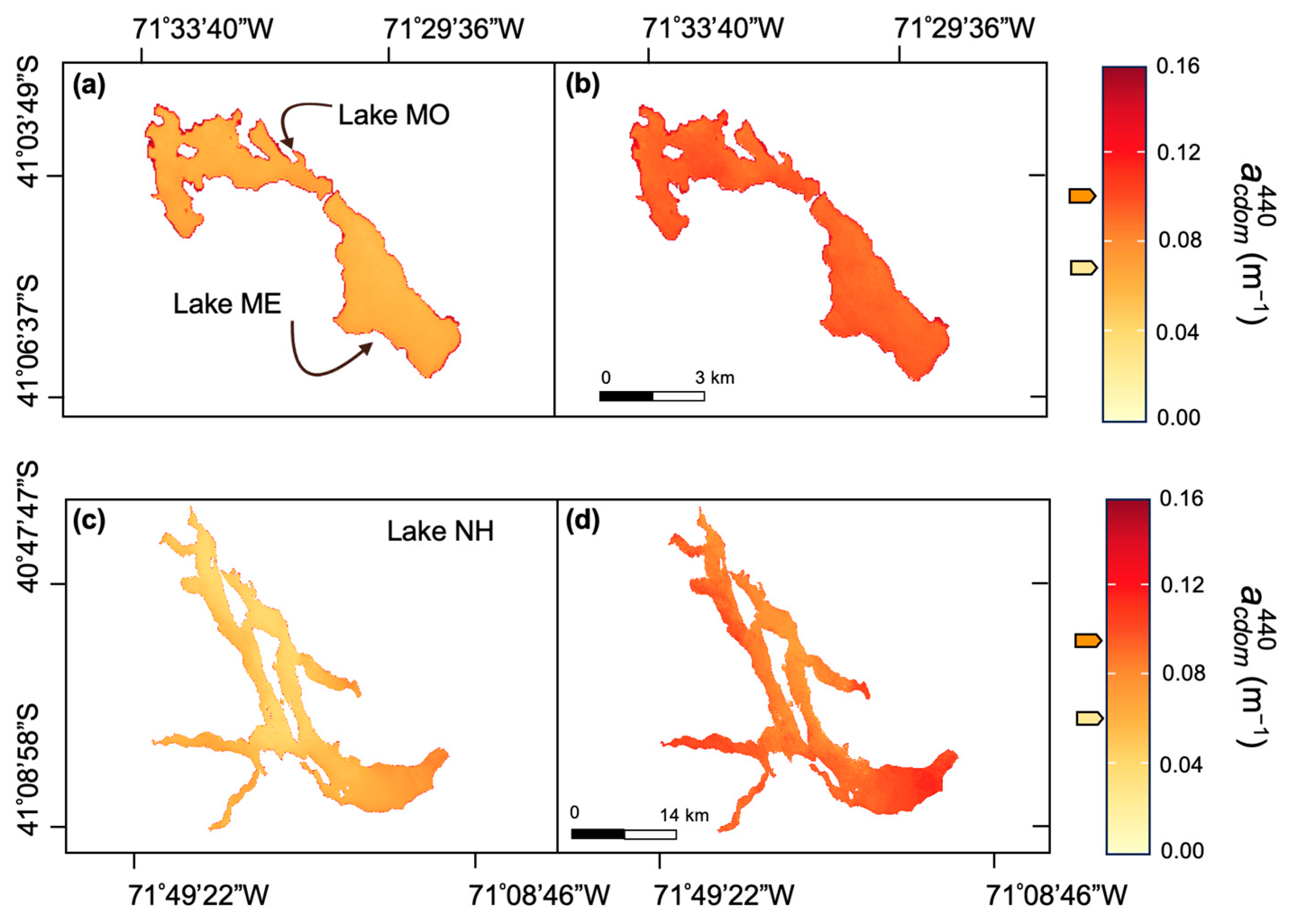
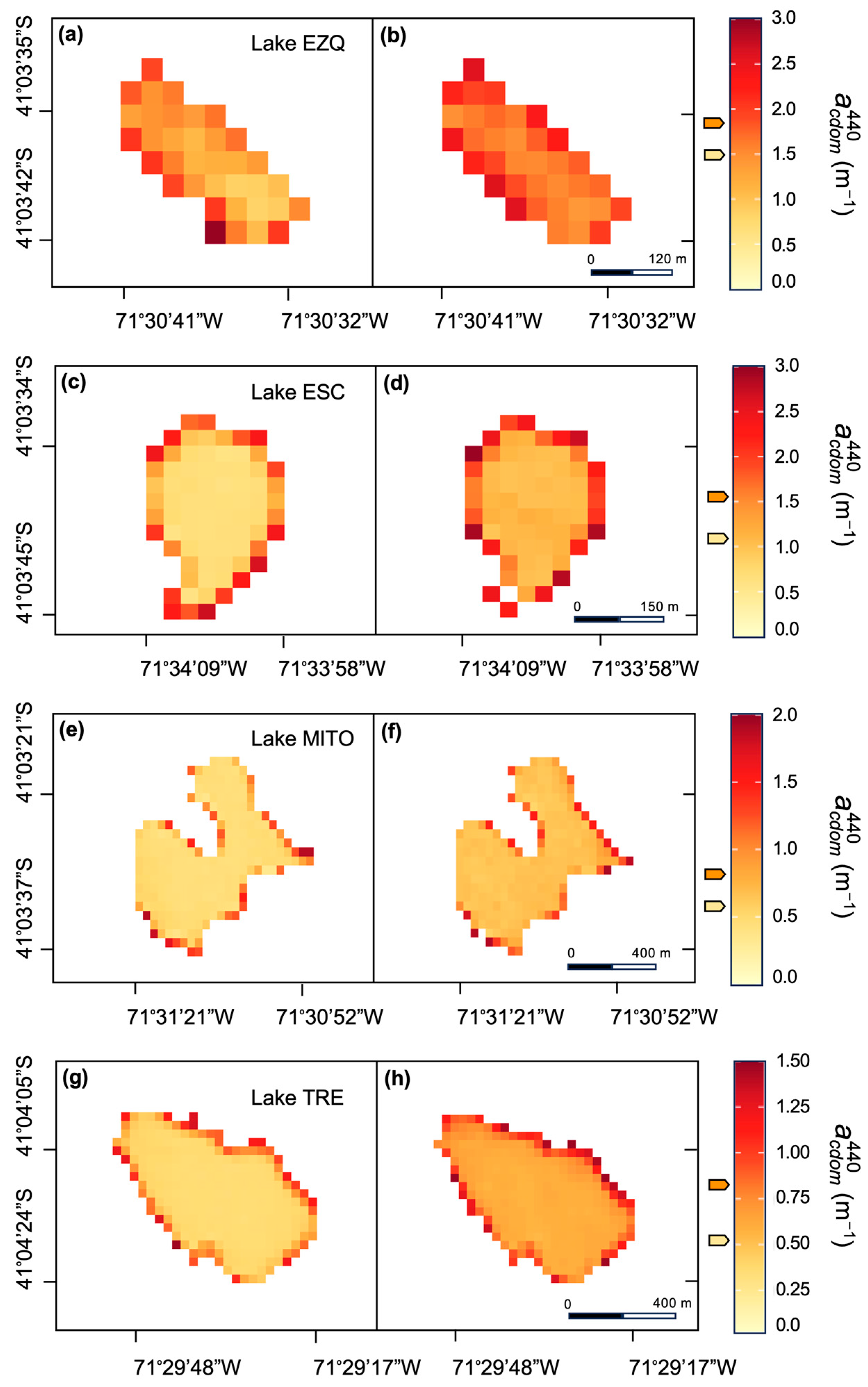
3.3. Spatio-Temporal Variability of CDOM in Study North Andean Patagonian Lakes

Lake type-specific models of QUAC routine were applied to 40 nearly cloud-free Landsat 8 images acquired during the 2016–2020 period. From the processed images, a total of 531 records of satellite-derived $a_{cdom}^{440}$ values from 3 × 3 pixel window scenes were used to analyze the spatio-temporal variability of CDOM in the study lakes. Since the northwestern Patagonian region commonly presented very abundant cloudiness and strong winds, it was not possible to obtain clear scenes for each month during the five-years study period (for a more detailed explanation of image and scene processing, refer to Section 2.6). Therefore, we focussed the analysis of CDOM seasonality on calculating the monthly mean CDOM concentrations for a 12-month interval (from January to December) using obtained satellite-derived $a_{cdom}^{440}$ values from 3 × 3 pixel window scenes for the 2016–2020 period. On average, three images per month were obtained (eight per year), except for September and October, where only one cloud-free image for each month was acquired. The limitation in the frequency of Landsat imagery did not allow for a reliable evaluation of inter-annual variability of CDOM during the evaluated period in this study.

In Figure 3, boxplots show the satellite-derived $a_{cdom}^{440}$ values at each sampled site per lake ordered from higher to lower mean values, closely reproducing the observed in situ inter-lake variation in CDOM (see Table 1).

Satellite-derived $a_{cdom}^{440}$ values ranged widely from 0.022 m⁻¹ in NH to 2.46 m⁻¹ in EZQ, representing a coefficient of variation of 138%. On average, satellite-derived ${a }_{cdom}^{440}$ values of deep lakes were 18% higher than in situ observations and 10% lower in shallow lakes (except for TRE). In this lake, the satellite-derived $a_{cdom }^{440}$ values were on average 37% higher than those observed in situ. The performance of our empirical algorithm in TRE and the relationship with the observed underwater light climate in this lake is discussed later in Section 4.1.

Besides differences in the retrieved CDOM among lakes, a clear intra-lake variation was observed in each of the study lakes (Figure 3). This variation represents seasonal and interannual differences in CDOM concentration during the 2016–2020 period. Even if temporal variability in each of the study lakes was lower that the observed differences among lakes, satellite-derived CDOM values showed a clear seasonal pattern. In deep lakes, lower monthly mean $a_{cdom}^{440}$ values, relative to the average value for the 12-month period, were observed from January to April (Figure 4). In contrast, equal to or higher monthly means were observed between May and December, apart from August in NH (Figure 4a).

Similarly, shallow lakes EZQ and ESC presented lower monthly mean values in a slightly longer time, between February to June, and equal to or higher during the July–January period (Figure 5a,b). Regarding lakes MITO and TRE, lower monthly mean values were observed between February to April and mean values equal to or higher during the May–January interval (Figure 5c,d). From the above-described temporal variation in retrieved values of $a_{cdom}^{440}$, two periods of low and high CDOM levels can be clearly established for the deep and shallow study lakes. Deep lakes presented significantly lower mean $a_{cdom}^{440}$ values during the January–April period than the May–December one (KW-ANOVA, p < 0.05; Figure S2). Similarly, shallow lakes EZQ and ESC showed significant lower mean values during February–June than during the July–January period (KW-ANOVA, p < 0.05; Figure S2). Particularly, lakes MITO and TRE presented a shorter period of low CDOM levels, with significantly lower mean $a_{cdom}^{440}$ values during the February–April period than the May–January one (KW-ANOVA, p < 0.05, Figure S2).

The previously outlined spatio-temporal variation of CDOM on a monthly scale, observed for 3 × 3 pixel scenes in each study lake, was also noticeable for the entire lake extent. CDOM algorithms were applied to Landsat 8 images, obtaining a good quality mapping of lacustrine $a_{cdom}^{440}$ values at a 30 m spatial resolution. A synoptic view of CDOM seasonality was achieved by separately mapping the low and high CDOM periods by lake, showing clear differences between seasons at the lake level (Figure 6 and Figure 7). In general, lakes showed an even distribution of CDOM concentration in their surface waters. Particularly, the generated maps were observed to perform poorly at the lakes’ edges. This issue was likely due to adjacency effects and the influence of shallow waters in the margin areas that interfered with the reflectance values.

3.4. Relationships Between Environmental Variables and CDOM Dynamics in North Andean Patagonian Lakes

3.4.1. Meteorological Features and Water Storage

Throughout the five-year study period, variations in air temperature, precipitation, and water storage revealed the marked weather seasonality characteristic of the North Andean Patagonian region (Figure 8). Mean daily air temperature was 8.41 ± 5.03 °C, showing a clear pattern with higher values during the December–February period (13.98 ± 1.15 °C) and lower values during the June–August period (3.07 ± 0.90 °C). In contrast, rain precipitation presented an opposite seasonality. Mean cumulative rain precipitation was 80.92 ± 68.29 mm, with 5-fold higher mean values during cold months (160.20 ± 75.82 mm) than during warm months (30.43 ± 22.24 mm). Mean daily wind speed was high (12.19 ± 6.27 Km h⁻¹), with a Northwest-predominant direction. Higher wind speed was observed during the October–February period (14.74 ± 1.70 Km h⁻¹) and lower during the April–July period (8.89 ± 1.64 Km h⁻¹).

Water storage of Lake Nahuel Huapi showed a clear seasonality (Figure 8). Regardless of the interannual variation, the lowest values for water storage were observed before the beginning of rainy months (between March and April), followed by a first maxima during or after the highest rain precipitation events (between July and September). A second and commonly higher water storage maxima was observed during the October–November period produced by the spring snow melting (Figure 8). Concerning solar irradiation and UV index, the study site also presented, as expected, a clear seasonality similar to that observed for air temperature. Mean irradiation value during the study period was 136.78 ± 69.04 KW m⁻², ranging between 37.69 KW m⁻² in June and 242.69 KW m⁻² in January. The UV index (dimensionless) showed a mean daily value of 0.98 ± 0.68, ranging from 0.056 in July to 2.63 in January.

Differences in some evaluated meteorological variables were observed between years. Annual cumulative rain precipitation showed the lowest value in 2016 (672.6 mm) and highest value in 2017 (1340 mm). The lowest annual water storage was registered in 2016 (5170 hm³), but the highest annual value was observed in 2018 (9159 hm³). On a monthly scale, the maximum water storage values were observed in November of 2017 (1001 hm³) and 2018 (1127 hm³), while a minimum monthly value was recorded in June of 2016 (178.9 hm³).

3.4.2. Lake Hydrogeomorphic and Watershed Features

A noteworthy difference in lake hydrogeomorphic features and catchment characteristics were observed among the study lakes, representative of the important variability in lacustrine environments present in Nahuel Huapi National Park. Lake area of shallow lakes ranged from 0.042 km² in EZQ to 0.33 km² in MITO (

Table 4. Description of the hydrogeomorphic and catchment characteristics, assessed as static variables, of the six study lakes. These parameters were evaluated as explanatory variables for the spatio-temporal variability of the satellite-derived $a_{cdom}^{440} \mathrm{v}\mathrm{a}\mathrm{l}\mathrm{u}\mathrm{e}\mathrm{s}$. References to the source of information are also provided.

Hydrogeomorphic and Catchment Characteristics	Lake Escondido	Lake Trébol	Lake Ezquerra	Lake Morenito	Lake Moreno E.	Lake Moreno O.	Lake Nahuel Huapi
Lake perimeter [Km]	1.46 [54]	2.27 [76]	0.88 [77]	3.98 [54]	13.30 [81]	19.30 [81]	357.40 [78]
Lake area [Km2]	0.09 [54]	0.31 [76]	0.42 × 10−1 [77]	0.33 [54]	6.14 [81]	6.10 [81]	557.00 [78]
Lake peri./lake area [Km−1]	16.13	7.32	20.70	12.09	2.16	3.16	0.64
Lake volume [Km3]	0.50 × 10−3 [54]	0.14 × 10−2 [85]	0.79 × 10−4 [77]	1.55 × 10−3 [54]	0.41 [81]	0.20 [81]	87.46 [82]
ZMAX [m]	8.05 [54]	12.00 [79]	3.60 [77]	12.00 [79]	106.00 [81]	90.00 [81]	454.00 [78]
ZAVG [m]	5.10 [54]	6.20 [85]	1.84 [77]	5.10 [54]	67.00 [81]	33.50 [81]	156.10 [85]
WRT [years]	0.56 [54]	1.23 [84]	0.09 [77,83]	0.50 [54]	2.29 [81]	0.98 [81]	16.56 [85]
Watershed area [Km2]	0.42 [54]	1.85 [80]	0.06 [83]	1.49 [54]	116.93 [81]	23.77 [81]	4260.00 [78]
Wshd. area/lake volume [Km−1]	838.00	1321.43	769.62	961.29	285.19	118.85	48.71

). In deep lakes, lake area varied more widely, with MO presenting an area of 6.1 km² and NH an area of 557 km². Similarly, lake perimeter and lake volume of shallow lakes varied from 0.88 km and 0.79 × 10⁻⁴ Km³ in EZQ to 3.98 km and 1.55 × 10⁻³ Km³ in MITO. In deep lakes, perimeter and volume ranged from 13.3 km and 0.2 km³ in lakes ME and MO, respectively, to 357.4 km and 87.46 km³ in NH. The lake perimeter to lake area ratio of shallow lakes varied between 7.32 km⁻¹ in TRE to 20.7 km⁻¹ in EZQ. In deep lakes, this ratio ranged from 0.64 km⁻¹ in NH to 3.16 km⁻¹ in MO. Regarding lake depth maxima (Z_MAX) and lake depth average (Z_AVG), in shallow lakes these features ranged from 3.6 m and 1.84 m in EZQ to 12 m and 6.20 m in TRE. In deep lakes, Z_MAX and Z_AVG varied from 90 m and 33.5 m in MO to 454 m and 156 m in NH. Water residence time (WRT) was minimum in EZQ (0.09 years) and maximum in NH (16.59 years) (Table 4). Concerning catchment characteristics, watershed area of shallow lakes varied between 0.06 Km² in EZQ to 1.85 Km² in TRE. In deep, large lakes, watershed area ranged from 23.8 Km² in MO to 4260 Km² in NH. The ratio between watershed area and lake volume ranged from 48.7 km⁻¹ in NH to 1321.3 km⁻¹ in TRE.

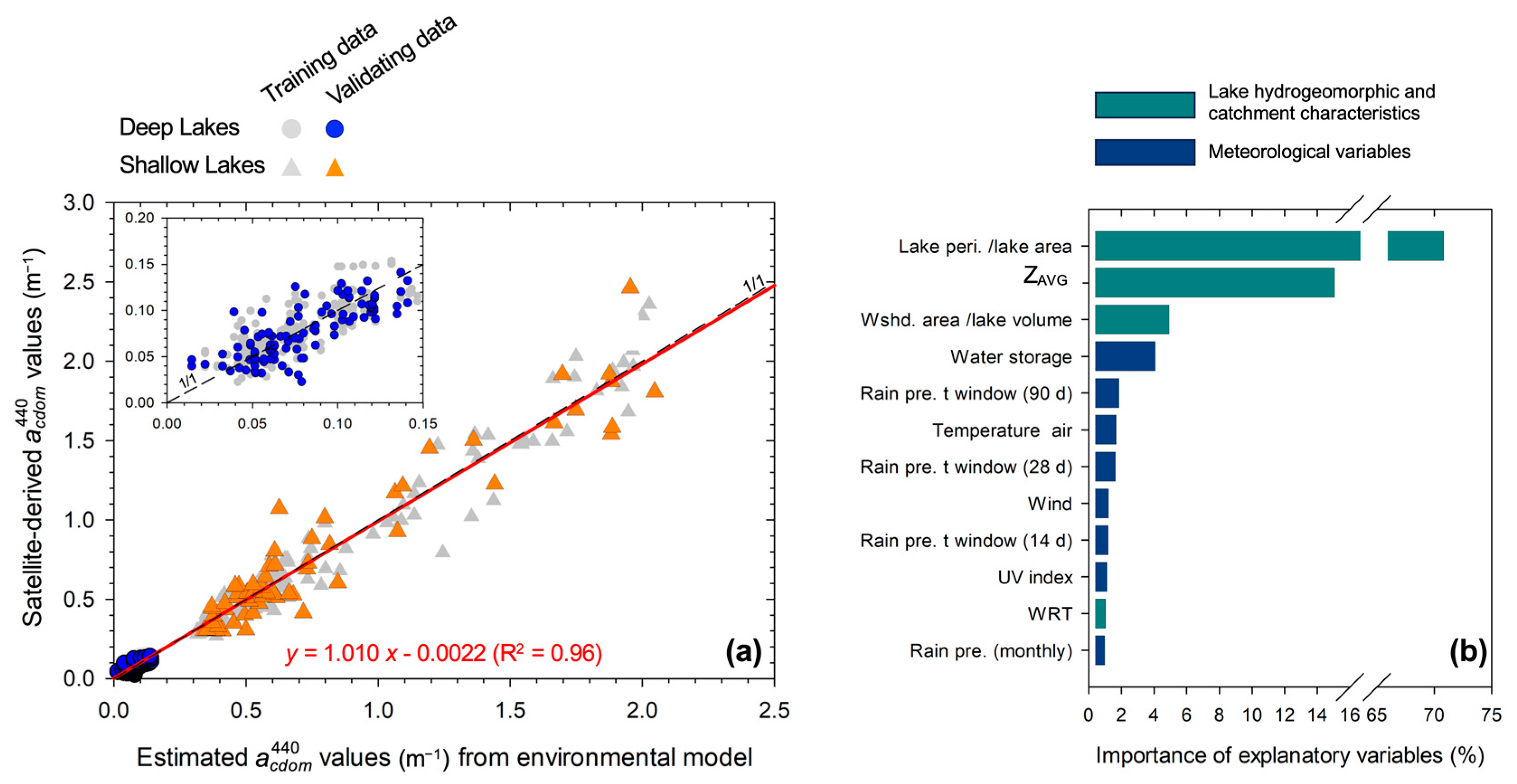
3.4.3. Drivers of CDOM Spatio-Temporal Variability

We investigated the influence of various environmental factors on the spatio-temporal variability of satellite-derived CDOM concentration in the lakes under study. These factors included hydrogeomorphic lake features (such as area, perimeter, volume, depth, water storage, and WRT), catchment features (such as watershed area and watershed area to lake volume ratio), and time series of meteorological features (such as air temperature, precipitation, wind speed, irradiation, and UV index). A total of 12 out of 21 environmental variables were used in the assessed machine learning technique, gradient boosted regression machine (GBRT). GBRT is generally robust to collinearity, which refers to the high correlation between predictor variables in a regression problem. However, to ensure easy model interpretation, we excluded variables with high correlation. For example, lake area, lake perimeter, and lake volume were highly correlated with each other (r > |0.80|) as well as with the lake perimeter to lake area ratio. The latter demonstrated a stronger correlation with satellite-derived $a_{cdom}^{440}$ values than the other three lake features and therefore was included in the analysis. In terms of meteorological variables, cumulative rain precipitation within 7-, 21-, and 60-day time windows showed lower correlation than rain precipitation within 14-, 30-, and 90-day time windows (r > 0.6). Therefore, the former three rain time windows were excluded. Similarly, the UV index and solar radiation were highly correlated (r > 0.93), though UV index presented a stronger correlation with the independent variable and was kept in the analysis.

The GBRT model explained a significant portion of the variation in satellite-derived $a_{cdom}^{440}$ values (R² = 0.96), with moderate errors (RMSE = 0.095 m⁻¹, MAPE = 22%) for the validation dataset (Figure 9a). This environmental model was designed for the deep and shallow lakes together, covering a wide range of CDOM concentrations. However, GBRT also produced good results when focusing on low $a_{cdom}^{440}$ values (deep lakes), with a lower regression coefficient (R² = 0.61) but still moderate errors (RMSE = 0.020 m⁻¹, MAPE = 26%) for the validation dataset. For shallow lakes only, the GBRT model demonstrated accurate performance with an R² value of 0.92 and low errors (RMSE = 0.155 m⁻¹, MAPE = 16%) for the validation dataset.

The hydrogeomorphic lake and watershed features, including the lake perimeter to lake area ratio, Z_AVG, watershed area to lake volume ratio, and lake water storage, were found to be the most significant environmental variables in explaining the observed spatio-temporal variability of surface waters CDOM in this study (with a relative importance of around 90%, as shown in Figure 9b). In contrast, time series of meteorological variables, including rain precipitation in a time window of 90, 28, and 14 days; air temperature; wind speed; and UV index, played a comparatively lower role (relative importance ~10%) (Figure 9b). It is worth noting that the lake perimeter to lake area ratio was the most important explanatory variable, showing a strong positive relationship with satellite-derived $a_{cdom}^{440}$ values (R² = 0.79). However, with the exception of the lake water storage, the lake perimeter to lake area ratio, together with other specific lake and catchment characteristics (Z_AVG and wshd. area/lake volume), were assessed as static variables. This means that they varied among lakes but not over time. Therefore, these characteristics strongly explain differences in CDOM concentration between the study lakes (inter-lake differences). On the other hand, water storage, together with cumulative rain precipitation (within a 90-day window) and air temperature, as well as other dynamic meteorological variables, effectively explained the temporal variability of CDOM in each lake (intra-lake differences).

Insights into the type of relationship between the target variable (satellite-derived $a_{cdom}^{440}$ values) and one or more input features (environmental drivers) can be interpreted from the partial dependence plots, which control the effects of other features (see Figure 10). These plots suggest that the lake perimeter to lake area ratio, watershed area to lake volume ratio, water storage, and rain precipitation in a 90-day window (Figure 10a, Figure 10c, Figure 10d and Figure 10e, respectively) had a positive effect on CDOM. Conversely, Z_AVG and air temperature had a negative effect on CDOM (Figure 10b and Figure 10f, respectively). Other variables, such as wind speed and WRT, had a non-linear relationship with CDOM, although the UV index and rain precipitation in 28- and 14-day windows had a positive effect (Figure S4).

4. Discussion

4.1. Remote Sensing of CDOM in Inland Waters: From Clear to Brown Lakes

The remote sensing of CDOM in inland waters has been significantly advanced by the growing demand for accurate estimates of the aquatic carbon budget at appropriate spatio-temporal scales. This arises in relation to the current consensus on the crucial role of inland waters in the global carbon cycle [1,4,97]. Despite the motivation behind this research topic, the goal of achieving a global estimate of CDOM using remote sensing, and indirectly of DOC concentration at continental or global scales, remains elusive. Among various difficulties that have hampered remote sensing of water quality in inland waters and particularly of CDOM [23,24,33], one that stands out is the fact that there are currently no satellites specifically designed to observe inland waters. Consequently, data from sensors designed for terrestrial or marine applications are employed to investigate water quality, with the specific characteristics of these sensors adapted to the complex aquatic environment [73,98,99,100,101].

Notwithstanding the peculiarities affecting remote sensing estimation of CDOM, several studies in inland waters have reported moderate to good results using empirical band ratio models [29,102,103]. However, these investigations showed a significant heterogeneity in the key issues for the development of remote sensing algorithms, making it difficult to draw clear generalizations and conclusions. For example, several studies implemented a single band ratio to retrieve CDOM absorption [28,30,31,35], although others used a two-term model of band and band ratio [37,38,104]. More complex models implementing machine learning methods have also been reported with promising results [105,106,107]. Furthermore, different data inputs (TOA, BOA, surface reflectance, remote sensing reflectance) and atmospheric corrections have been commonly used [40,108,109].

In addition to the methodological variability described above, it is important to note that there is still a lack of research analyzing remote sensing of CDOM in lakes with very low to low CDOM concentrations. Various investigations have compiled in situ measurements of CDOM in inland waters on a global scale [110,111,112]. However, these databases are not yet representative of the majority of continental water bodies. For example, lakes in Argentine and Chilean Andean Patagonia are seldom represented, as these waters are characterized by very low to moderate CDOM concentrations [49,113]. To the best of our knowledge, only a few papers have focused on the remote sensing of low CDOM concentrations in inland waters [40]. These authors conducted a study on waters from the Sacramento River and Lake Erie and found that the blue/red band ratio of Landsat 8 remote sensing reflectance was the best model for predicting low CDOM values (mean $a_{cdom}^{440}$ = 0.524 m⁻¹; range 0.07–1.24 m⁻¹). They observed that in these low-coloured waters, the optimal short band was changed from green to blue. This is because CDOM absorption at blue wavelengths may contribute a greater proportion of the total absorption budget than at other higher wavelengths.

Our work supports that of Chen et al. [40]. We found that in deep Andean lakes with very low CDOM concentrations (mean $a_{cdom}^{440}$ = 0.06 m⁻¹; range 0.027–0.106 m⁻¹), the best two-term model using surface reflectance and QUAC atmospheric correction included the blue/red band ratio. This band combination alone explained 72% of the observed variability in ln $a_{cdom}^{440}$. In these waters, CDOM absorption commonly accounted for over 60% of the total absorption budget at blue wavelengths [50]. However, given the low concentration of CDOM, the water leaving signal remained strong at these wavelengths, resulting in relatively high signal-to-noise ratios. Our findings suggest that remote sensing can detect CDOM values lower than those assessed by Chen et al. [40], expanding the range of investigation for this important water quality variable from space.

Regarding shallow North Andean Patagonian lakes, the outcomes presented here are consistent with previous studies that have found the green/red band ratio to be the most effective band combination for retrieving CDOM in waters with moderate to high concentrations of this optically active substance. In the shallow study lakes, CDOM presented low to moderate concentrations (mean $a_{cdom}^{440}$ = 0.78 m⁻¹; range 0.23–2.04 m⁻¹), and the green/red band ratio alone accounted for 78% of the observed variation in ln $a_{cdom}^{440}$. Absorption at blue wavelengths in these waters was approximately five times higher than in deep Andean Patagonian lakes. As a result, the signal-to-noise ratio at this spectral region was decreased due to the combined absorption of CDOM and suspended particles. However, in shallow lakes (excluding Lake Trébol), CDOM still dominated the absorption budget at green wavelengths, albeit with much lower absolute values than at the blue spectral region. This makes it possible to estimate CDOM in these waters using the green band. Lake Trébol presents a similar contribution of both CDOM and suspended particles to the absorption process between 460 and 580 nm (refer to Figure S1c). This has been previously described by [50,114]. Estimating CDOM from space in this water body, and others with similar underwater light climates, may be challenging due to either high absorption coefficients at blue wavelengths or the significant absorption contribution of particles at green wavelengths. In particular, this could explain the higher satellite-derived $a_{cdom}^{440}$ values in Lake Trébol compared to those observed in situ. These results emphasize the significance of accurately characterizing the optical properties of inland water bodies to improve remote sensing estimation of water quality parameters. In addition, satellite remote sensing of CDOM in shallow Andean Patagonian lakes seems likely to be less sensitive than deep lakes to atmospheric conditions. All the evaluated atmospheric correction routines selected the green/red band ratio (or its reciprocal), with TOA reflectance performing as well as the best model using QUAC. This has been previously reported by different authors showing comparatively good results using either TOA reflectance or atmospherically corrected images in lakes presenting moderate to high CDOM concentrations [36,115].

Our research also demonstrates that the algorithms developed in this study provide improved estimates of CDOM compared to previously published models in the specific context of our study lakes. Notably, both our models and those of Kutser et al. [39] and Alcântara et al. [96] showed strong performance when using the blue/red band ratio for deep lakes and the green/red band ratio for shallow lakes. This indicates the sensitivity of the blue and green spectral regions of satellite imagery to accurately describe CDOM in the concentration ranges that characterize inland waters and suggests that tailoring remote sensing algorithms to the unique optical characteristics of different lake types can improve the accuracy of CDOM estimates. As previously stated by Chen et al. [40], a future direction for simultaneously estimating very low to very high CDOM lacustrine concentrations could be the development of empirical models based on optical classification of water bodies. Several authors have demonstrated that the remote estimation of CDOM can be enhanced by dividing datasets based on trophic status [116], chlorophyll a concentration [117], and turbidity levels [118]. In our study, when deep and shallow lakes were analyzed separately, empirical models exhibited a significant improvement in CDOM estimation. The application of specific models for lake types resulted in a reduction of MAPE by approximately 53% for shallow lakes and 70% for deep lakes, in comparison to all lakes pooled together. Moreover, it is evident that the classification of the studied Andean Patagonian lakes based on their morphometric parameters (i.e., deep large and shallow small lakes) is associated with distinct difference in their underwater optical characteristics. This emphasizes the necessity for the utilization of distinct remote sensing models (i.e., different band combinations) to accurately estimate CDOM from space.

Our evaluation of different atmospheric correction methods revealed that empirical and physically based approaches, such as QUAC and DOS1, provided the most accurate estimations of CDOM concentrations in the clear waters of the Andean Patagonian lakes. QUAC showed superior performance, likely due to its flexibility in adapting to the optical properties of the region without relying on detailed atmospheric data [68]. In contrast, more complex methods like L2gen and LaSRC performed less effectively. L2gen faced limitations in clear waters due to aerosol selection errors, adjacency effects, and low signal-to-noise ratios in the blue and green bands [119,120]. Accurate aerosol information is crucial for high-quality reflectance retrievals [69], and environmental factors like solar zenith angle and wind speed can affect its accuracy. Furthermore, LaSRC has shown to be less accurate in inland waters, particularly in the blue bands, as it estimates aerosols over land and extrapolates these estimates over water, leading to inaccuracies [120].

4.2. Spatio-Temporal Variability of CDOM in North Andean Patagonian Lakes and Its Main Driving Forces

Given the active role of inland waters in the carbon cycle, it is crucial to understand the spatio-temporal dynamics of DOM, as well as its main drivers and sink processes, to improve estimates of carbon stocks in lakes [1,3,121,122,123]. This understanding can also aid researchers in assessing the potential impacts of environmental changes, such as climate change, on lacustrine biogeochemistry and other important processes mediated by CDOM, such as water transparency and the quality of drinking water, among others.

Measuring the extent of spatial and temporal variability in ecosystems’ characteristics is the initial step towards understanding ecological processes [124]. This task is particularly challenging for ecosystem properties that are influenced by various factors operating at different scales. An example of such ecosystem properties is the concentration of DOM in lakes. It acts as an indicator of the impact of landscapes on lakes and mirrors a multitude of processes occurring in both terrestrial and aquatic environments [14].

In landscapes where wetlands or forests predominate, lacustrine DOM is mainly derived from terrestrial sources rather than being primarily generated within the lake through internal processes [125,126,127]. Allochthonous DOM inputs from the surrounding watershed are connected to the lake through surface runoff and groundwater inflows. Meteorological conditions, therefore, can strongly affect these hydrological inputs. Alterations in rainfall patterns have a significant impact on the delivery of DOM to aquatic ecosystems. Consequently, climate change could influence DOM inputs to lakes, as significant reductions in DOM can occur during dry periods [128,129,130]. Conversely, increases in precipitation on annual or shorter time scales lead to counteracting effects by promoting carbon exports from the drainage network to lake waters [131,132,133]. In addition to the direct link between precipitation and DOM concentration in aquatic environments, several studies have reported the importance of other climatic variables (or those related with) as drivers of seasonal and interannual variability of DOM. For example, air temperature [134,135], solar radiation [136,137], and lake water level [89] have been identified as key drivers of DOM concentration. Furthermore, auxiliary variables related to weather, such as ice-out dates, day of year, month, and the duration of the growing and runoff seasons, have been also demonstrated to explain temporal variability in DOM [131,134,138].

At the spatial scale, catchment characteristics (e.g., soil type, vegetation cover, drainage extent, etc.) and lake features (e.g., lake area, perimeter, volume, altitude, WRT, etc.) have been found to be significant drivers of inter-lake differences in either DOC or CDOM concentrations. For example, a global study showed that altitude was the most important feature explaining the spatial variation of DOC [139,140]. However, when the global lake data were divided into regional subsets, other catchment and lake characteristics (e.g., lake area to drainage area ratio) explained a significant amount of DOC variability [139]. Similarly, Xenopoulos and Schindler [141] found that in northern temperate lakes from the Upper Great Lakes region, DOC variability was mainly explained by the lake and watershed properties (i.e., the proportion of lake perimeter and catchment occupied by wetlands).

From the above evidence, it can be concluded that the dynamics of DOM in lacustrine ecosystems are influenced by a complex interplay of spatio-temporal factors. Of particular note is the important role that catchments and lake characteristics play in modulating the impact of climatic forces on DOM dynamics. Our research provides a compelling illustration of how lake and watershed characteristics interact with climatic forces to shape CDOM spatio-temporal variability. Over a five-year period, we identified the lake perimeter to lake area ratio, Z_AVG, watershed area to lake volume ratio, and water storage as the most important parameters explaining the observed spatio-temporal variability in CDOM in the surface waters of the six study lakes. It is noteworthy that the first three variables (assessed as static variables) were instrumental in explaining the differences in satellite-derived $a_{cdom}^{440}$ values among lakes. These inter-lake differences constituted the primary source of CDOM variability in our dataset, representing a coefficient of variation of 135%. In contrast, the temporal variability (reflected in CDOM differences within each lake) was comparatively lower, with values ranging from 21% in Lake EZQ to 43% in Lake NH. This intra-lake variability generally followed a coherent pattern among lakes, with lower satellite-derived $a_{cdom}^{440}$ values typically observed during the summer to early autumn period and higher values during the winter to spring period. This synchrony was largely attributed to lake water storage, which serves as a proxy for the seasonal and interannual variations in water levels at the local scale, followed by the cumulative rain precipitation in a 90-day window and the air temperature. Lake water storage likely integrates the effects of both winter precipitation and spring snowmelt, which dictate the timing and amplitude of DOM pulses into the lakes. In summer, an abrupt drop in water level leads to a significant reduction in the transfer pathways of dissolved carbon between terrestrial and aquatic environments. This is followed by an increase in photodegradation processes within the lakes, induced by higher UV irradiance levels, leading to a decrease in the average molecular size of DOM and a progressive loss of colour in lake surface waters.

In our model, while the most important variables demonstrated clear and expected relationships with CDOM, some of the less important variables, such as the alternative rainfall windows (of 14 and 28 days), also showed straightforward relations. These rainfall windows may be indicative of different CDOM input pulses, like the dissimilar responses of DOC to precipitation events observed by Warner and Saros [142] in boreal lakes. However, certain evaluated variables, such as WRT and UV index, yielded results that were less intuitive. The wide range of WRT values across the lakes (from 0.09 to 16 years) may have obscured the effect of this variable. Lake Nahuel Huapi exhibited a significant deviation in WRT from the mean. The positive relationship between UV index and CDOM observed in the partial dependence plots may reflect complex interactions with other environmental variables, which warrant further investigation in future studies.

It is important to emphasize that the environmental model presented in this paper is a simplified model. The evaluated hydrogeomorphic characteristics of the lakes are in fact parameters with a temporal variability, and although these should covary in some way with the main forcing meteorological variables, the inclusion of this dynamic in future environmental models could improve the description of the spatio-temporal variability of the lacustrine CDOM. On the other hand, the use of the water storage of Lake Nahuel Huapi as a reference for the seasonal variability of the water levels in the study lakes is also a simplification, and its temporal evaluation for each lake could significantly improve the description of the CDOM seasonality in the study lakes. Radar and laser altimeter satellites are valuable tools for describing seasonal variations in lake water levels. However, these instruments have limitations in spatial and temporal scales, primarily due to land coverage and revisit times, which can hinder the study of small lakes or the detailed analysis of water level seasonality in large lakes [143,144]. The launch of the SWOT (Surface Water and Ocean Topography) satellite in December 2022 is expected to significantly enhance the description of this critical variable in the study area, enabling a more detailed understanding of the key environmental factors that influence CDOM spatio-temporal variability in North Andean lakes.

This investigation aligns with previous studies of Andean Patagonian lakes. Research in this mountainous region, focusing on the optical properties of DOM, has highlighted strong terrestrial–aquatic linkages, showing a dominant contribution of terrestrial DOM to the carbon pool in headwaters and lakes [54,145,146]. Additionally, the seasonality of DOM has been strongly linked to climate forcing variables. Terrestrial inputs of both dissolved and particulate organic material increase with precipitation, which enhances runoff during the wet season, whereas dry periods are characterized by lower hydrological connectivity and increased photobleaching of lacustrine CDOM [55,56,83]. Furthermore, research has demonstrated the modulating role of hydrogeomorphic and watershed characteristics on lake responses to climate forcings as well as the influence of landscape heterogeneity driven by strong bioclimatic gradients on DOM properties [42,79,82,113].

The use of remote sensing in the North Andean Patagonian lakes has allowed for a more detailed analysis of CDOM seasonality at a previously unexplored temporal scale. However, high cloud cover and strong winds in this geographical area limited the assessment of interannual CDOM variability using Landsat 8 imagery. Cloud cover significantly limited the number of usable scenes for each month during the study period from 2016 to 2020, where an average of only three images per month were available, and in some months, such as September and October, only one cloud-free image was obtained. The implementation of Landsat 9, in combination with Landsat 8 starting from November 2021 in the study area, is expected to significantly increase the availability of clear satellite imagery. This improved temporal coverage will facilitate more frequent and consistent monitoring of CDOM concentrations, thereby enhancing the temporal resolution of the analysis. Additionally, future research could benefit from incorporating satellite systems with even higher temporal resolution, such as Sentinel-2, or applying more advanced cloud-masking techniques to further address the challenges of cloud cover, which is particularly prevalent in regions like Patagonia.

Characterizing the natural variability of CDOM in these aquatic ecosystems provides a basis for establishing benchmarks to identify and quantify the impacts of climate change and other anthropogenic alterations on the lake environment. This information enhances the ability to estimate lacustrine carbon stocks at a regional scale and is crucial for long-term planning and decision making in the context of environmental change.

References

1. Cole, J.J.; Prairie, Y.T.; Caraco, N.F.; McDowell, W.H.; Tranvik, L.J.; Striegl, R.G.; Duarte, C.M.; Kortelainen, P.; Downing, J.A.; Middelburg, J.J.; et al. Plumbing the Global Carbon Cycle: Integrating Inland Waters into the Terrestrial Carbon Budget. Ecosystems 2007, 10, 172–185. [Google Scholar] [CrossRef]
2. Battin, T.J.; Luyssaert, S.; Kaplan, L.A.; Aufdenkampe, A.K.; Richter, A.; Tranvik, L.J. The Boundless Carbon Cycle. Nat. Geosci. 2009, 2, 598–600. [Google Scholar] [CrossRef]
3. Tranvik, L.J.; Cole, J.J.; Prairie, Y.T. The Study of Carbon in Inland Waters—From Isolated Ecosystems to Players in the Global Carbon Cycle. Limnol. Ocean. Lett. 2018, 3, 41–48. [Google Scholar] [CrossRef]
4. Regnier, P.; Resplandy, L.; Najjar, R.G.; Ciais, P. The Land-to-Ocean Loops of the Global Carbon Cycle. Nature 2022, 603, 401–410. [Google Scholar] [CrossRef] [PubMed]
5. Mehner, T. Encyclopedia of Inland Waters; Academic Press: Cambridge, MA, USA, 2009; ISBN 0123706262. [Google Scholar]
6. Ho, L.T.; Goethals, P.L.M. Opportunities and Challenges for the Sustainability of Lakes and Reservoirs in Relation to the Sustainable Development Goals (SDGs). Water 2019, 11, 1462. [Google Scholar] [CrossRef]
7. Aung, H.H. Preserving the cultural heritage a study of the Silversmith in Inlay lake, Myanmar. J. Myanmar Acad. Arts Sci. XVI 2018, 8, 131–158. [Google Scholar]
8. Reid, A.J.; Carlson, A.K.; Creed, I.F.; Eliason, E.J.; Gell, P.A.; Johnson, P.T.J.; Kidd, K.A.; MacCormack, T.J.; Olden, J.D.; Ormerod, S.J.; et al. Emerging Threats and Persistent Conservation Challenges for Freshwater Biodiversity. Biol. Rev. 2019, 94, 849–873. [Google Scholar] [CrossRef]
9. Dudgeon, D.; Arthington, A.H.; Gessner, M.O.; Kawabata, Z.-I.; Knowler, D.J.; Lévêque, C.; Naiman, R.J.; Prieur-Richard, A.-H.; Soto, D.; Stiassny, M.L.J.; et al. Freshwater Biodiversity: Importance, Threats, Status and Conservation Challenges. Biol. Rev. Camb. Philos. Soc. 2006, 81, 163–182. [Google Scholar] [CrossRef]
10. Williamson, C.E.; Brentrup, J.A.; Zhang, J.; Renwick, W.H.; Hargreaves, B.R.; Knoll, L.B.; Overholt, E.P.; Rose, K.C. Lakes as Sensors in the Landscape: Optical Metrics as Scalable Sentinel Responses to Climate Change. Limnol. Oceanogr. 2014, 59, 840–850. [Google Scholar] [CrossRef]
11. Williamson, C.E.; Dodds, W.; Kratz, T.K.; Palmer, M.A. Lakes and Streams as Sentinels of Environmental Change in Terrestrial and Atmospheric Processes. Front. Ecol. Environ. 2008, 6, 247–254. [Google Scholar] [CrossRef]
12. Adrian, R.; O’Reilly, C.M.; Zagarese, H.; Baines, S.B.; Hessen, D.O.; Keller, W.; Livingstone, D.M.; Sommaruga, R.; Straile, D.; Van Donk, E.; et al. Lakes as Sentinels of Climate Change. Limnol. Oceanogr. 2009, 54, 2283–2297. [Google Scholar] [CrossRef] [PubMed]
13. Woolway, R.I.; Kraemer, B.M.; Lenters, J.D.; Merchant, C.J.; O’Reilly, C.M.; Sharma, S. Global Lake Responses to Climate Change. Nat. Rev. Earth Environ. 2020, 1, 388–403. [Google Scholar] [CrossRef]
14. Williamson, C.E.; Saros, J.E.; Vincent, W.F.; Smol, J.P. Lakes and Reservoirs as Sentinels, Integrators, and Regulators of Climate Change. Limnol. Oceanogr. 2009, 54, 2273–2282. [Google Scholar] [CrossRef]
15. Yang, H.; Kong, J.; Hu, H.; Du, Y.; Gao, M.; Chen, F. A Review of Remote Sensing for Water Quality Retrieval: Progress and Challenges. Remote Sens. 2022, 14, 1770. [Google Scholar] [CrossRef]
16. Kirk, J.T.O. Light and Photosynthesis in Aquatic Ecosystems, 3rd ed.; Cambridge University Press: Cambridge, UK, 2011; ISBN 978-0-521-15175-7. [Google Scholar]
17. Wetzel, R.G. Limnology Lake and Reservoir Ecosystems, 3rd ed.; Academic Press: San Diego, CA, USA, 2001. [Google Scholar]
18. Häder, D.-P.; Kumar, H.D.; Smith, R.C.; Worrest, R.C. Effects of Solar UV Radiation on Aquatic Ecosystems and Interactions with Climate Change. Photochem. Photobiol. Sci. 2007, 6, 267–285. [Google Scholar] [CrossRef]
19. Perdue, E.M. Chemical Composition, Structure, and Metal Binding Properties BT—Aquatic Humic Substances: Ecology and Biogeochemistry; Hessen, D.O., Tranvik, L.J., Eds.; Springer: Berlin/Heidelberg, Germany, 1998; ISBN 978-3-662-03736-2. [Google Scholar]
20. Anderson, L.E.; Krkošek, W.H.; Stoddart, A.K.; Trueman, B.F.; Gagnon, G.A. Lake Recovery Through Reduced Sulfate Deposition: A New Paradigm for Drinking Water Treatment. Environ. Sci. Technol. 2017, 51, 1414–1422. [Google Scholar] [CrossRef]
21. Osburn, C.L.; Stedmon, C.A. Linking the Chemical and Optical Properties of Dissolved Organic Matter in the Baltic—North Sea Transition Zone to Differentiate Three Allochthonous Inputs. Mar. Chem. 2011, 126, 281–294. [Google Scholar] [CrossRef]
22. Spencer, R.G.M.; Butler, K.D.; Aiken, G.R. Dissolved Organic Carbon and Chromophoric Dissolved Organic Matter Properties of Rivers in the USA. J. Geophys. Res. Biogeosci. 2012, 117. [Google Scholar] [CrossRef]
23. Dekker, A.G.; Pinnel, N.; Gege, P.; Briottet, X.; Cour, A. Feasibility Study for an Aquatic Ecosystem Earth Observing System Version 1.2. In Feasibility Study for an Aquatic Ecosystem Earth Observing System; CEOS: Córdoba, Argentina, 2018. [Google Scholar]
24. Brezonik, P.L.; Olmanson, L.G.; Finlay, J.C.; Bauer, M.E. Factors Affecting the Measurement of CDOM by Remote Sensing of Optically Complex Inland Waters. Remote Sens. Environ. 2015, 157, 199–215. [Google Scholar] [CrossRef]
25. Zhu, W.; Yu, Q.; Tian, Y.Q.; Becker, B.L.; Zheng, T.; Carrick, H.J. An Assessment of Remote Sensing Algorithms for Colored Dissolved Organic Matter in Complex Freshwater Environments. Remote Sens. Environ. 2014, 140, 766–778. [Google Scholar] [CrossRef]
26. Matthews, M.; William Matthews, M. A Current Review of Empirical Procedures of Remote Sensing in Inland and Near-Coastal Transitional Waters. Int. J. Remote Sens. 2010, 32, 6855–6899. [Google Scholar] [CrossRef]
27. Li, J.; Yu, Q.; Tian, Y.Q.; Becker, B.L.; Siqueira, P.; Torbick, N. Spatio-Temporal Variations of CDOM in Shallow Inland Waters from a Semi-Analytical Inversion of Landsat-8. Remote Sens. Environ. 2018, 218, 189–200. [Google Scholar] [CrossRef]
28. Toming, K.; Kutser, T.; Laas, A.; Sepp, M.; Paavel, B.; Nõges, T. First Experiences in Mapping Lakewater Quality Parameters with Sentinel-2 MSI Imagery. Remote Sens. 2016, 8, 640. [Google Scholar] [CrossRef]
29. Olmanson, L.G.; Brezonik, P.L.; Finlay, J.C.; Bauer, M.E. Comparison of Landsat 8 and Landsat 7 for Regional Measurements of CDOM and Water Clarity in Lakes. Remote Sens. Environ. 2016, 185, 119–128. [Google Scholar] [CrossRef]
30. Chen, J.; Zhu, W.N.; Tian, Y.Q.; Yu, Q. Estimation of Colored Dissolved Organic Matter from Landsat-8 Imagery for Complex Inland Water: Case Study of Lake Huron. IEEE Trans. Geosci. Remote Sens. 2017, 55, 2201–2212. [Google Scholar] [CrossRef]
31. Chen, J.; Zhu, W.; Tian, Y.Q.; Yu, Q.; Zheng, Y.; Huang, L. Remote Estimation of Colored Dissolved Organic Matter and Chlorophyll-a in Lake Huron Using Sentinel-2 Measurements. J. Appl. Remote Sens. 2017, 11, 1. [Google Scholar] [CrossRef]
32. Al-Kharusi, E.S.; Tenenbaum, D.E.; Abdi, A.M.; Kutser, T.; Karlsson, J.; Bergström, A.-K.; Berggren, M. Large-Scale Retrieval of Coloured Dissolved Organic Matter in Northern Lakes Using Sentinel-2 Data. Remote Sens. 2020, 12, 157. [Google Scholar] [CrossRef]
33. Topp, S.N.; Pavelsky, T.M.; Jensen, D.; Simard, M.; Ross, M.R.V. Research Trends in the Use of Remote Sensing for Inland Water Quality Science: Moving towards Multidisciplinary Applications. Water 2020, 12, 169. [Google Scholar] [CrossRef]
34. Sagan, V.; Peterson, K.T.; Maimaitijiang, M.; Sidike, P.; Sloan, J.; Greeling, B.A.; Maalouf, S.; Adams, C. Monitoring Inland Water Quality Using Remote Sensing: Potential and Limitations of Spectral Indices, Bio-Optical Simulations, Machine Learning, and Cloud Computing. Earth Sci. Rev. 2020, 205, 103187. [Google Scholar] [CrossRef]
35. Kutser, T.; Casal, G.; Barbosa, C.; Paavel, B.; Renato, F.; Carvalho, L.; Toming, K. Mapping Inland Water Carbon Content with Landsat 8 Data. Int. J. Remote Sens. 2016, 37, 2950–2961. [Google Scholar] [CrossRef]
36. Kallio, K.; Attila, J.; Härmä, P.; Koponen, S.; Pulliainen, J.; Hyytiäinen, U.-M.; Pyhälahti, T. Landsat ETM+ Images in the Estimation of Seasonal Lake Water Quality in Boreal River Basins. Environ. Manag. 2008, 42, 511–522. [Google Scholar] [CrossRef] [PubMed]
37. Olmanson, L.G.; Page, B.P.; Finlay, J.C.; Brezonik, P.L.; Bauer, M.E.; Griffin, C.G.; Hozalski, R.M. Regional Measurements and Spatial/Temporal Analysis of CDOM in 10,000+ Optically Variable Minnesota Lakes Using Landsat 8 Imagery. Sci. Total Environ. 2020, 724, 138141. [Google Scholar] [CrossRef] [PubMed]
38. Koll-Egyed, T.; Cardille, J.A.; Deutsch, E. Multiple Images Improve Lake CDOM Estimation: Building Better Landsat 8 Empirical Algorithms across Southern Canada. Remote Sens. 2021, 13, 3615. [Google Scholar] [CrossRef]
39. Kutser, T.; Pierson, D.C.; Kallio, K.Y.; Reinart, A.; Sobek, S. Mapping Lake CDOM by Satellite Remote Sensing. Remote Sens. Environ. 2005, 94, 535–540. [Google Scholar] [CrossRef]
40. Chen, J.; Zhu, W.; Pang, S.; Cheng, Q. Applicability Evaluation of Landsat-8 for Estimating Low Concentration Colored Dissolved Organic Matter in Inland Water. Geocarto Int. 2019, 37, 1–15. [Google Scholar] [CrossRef]
41. Garcia, R.D.; Diéguez, M.d.C.; Gerea, M.; Garcia, P.E.; Reissig, M. Characterisation and Reactivity Continuum of Dissolved Organic Matter in Forested Headwater Catchments of Andean Patagonia. Freshw. Biol. 2018, 63, 1049–1062. [Google Scholar] [CrossRef]
42. Queimaliños, C.; Reissig, M.; Pérez, G.L.; Soto Cárdenas, C.; Gerea, M.; Garcia, P.E.; García, D.; Diéguez, M.C. Linking Landscape Heterogeneity with Lake Dissolved Organic Matter Properties Assessed through Absorbance and Fluorescence Spectroscopy: Spatial and Seasonal Patterns in Temperate Lakes of Southern Andes (Patagonia, Argentina). Sci. Total Environ. 2019, 686, 223–235. [Google Scholar] [CrossRef]
43. De Stefano, L.G.; Valdivia, A.S.; Gianello, D.; Gerea, M.; Reissig, M.; García, P.E.; García, R.D.; Soto Cárdenas, C.; Diéguez, M.C.; Queimaliños, C.P.; et al. Using CDOM Spectral Shape Information to Improve the Estimation of DOC Concentration in Inland Waters: A Case Study of Andean Patagonian Lakes. Sci. Total Environ. 2022, 824, 153752. [Google Scholar] [CrossRef]
44. Iriondo, M. Quaternary Lakes of Argentina. Palaeogeogr. Palaeoclim. Palaeoecol. 1989, 70, 81–88. [Google Scholar] [CrossRef]
45. Zagarese, H.E.; Diaz, M.; Pedrozo, F.; Úbeda, C. Mountain Lakes in Northwestern Patagonia. SIL Proceed. 1922–2010 2000, 27, 533–538. [Google Scholar] [CrossRef]
46. Diaz, M.; Pedrozo, F.; Reynolds, C.; Temporetti, P. Chemical Composition and the Nitrogen-Regulated Trophic State of Patagonian Lakes. Limnologica 2007, 37, 17–27. [Google Scholar] [CrossRef]
47. Pedrozo, F.; Chillrud, S.; Temporetti, P.; Diaz, M. Chemical Composition and Nutrient Limitation in Rivers and Lakes of Northern Patagonian Andes (39.5°-42° S; 71° W) (Rep. Argentina). SIL Proceed. 1922–2010 1993, 25, 207–214. [Google Scholar] [CrossRef]
48. Pérez, G.L. Optical Characterization of Argentinean Lakes, from Deep Andean Lakes to Shallow Pampean Ones. Adv. Limnol. 2014, 65, 409–430. [Google Scholar] [CrossRef]
49. Morris, D.P.; Zagarese, H.; Williamson, C.E.; Balseiro, E.G.; Hargreaves, B.R.; Modenutti, B.; Moeller, R.; Queimalinos, C. The Attenuation of Solar UV Radiation in Lakes and the Role of Dissolved Organic Carbon. Limnol. Oceanogr. 1995, 40, 1381–1391. [Google Scholar] [CrossRef]
50. Pérez, G.L.; Queimaliños, C.; Modenutti, B.E. Light Climate and Plankton in the Deep Chlorophyll Maxima in North Patagonian Andean Lakes. J. Plankton Res. 2002, 24, 591–599. [Google Scholar] [CrossRef]
51. Barros, V.R.; Boninsegna, J.A.; Camilloni, I.A.; Chidiak, M.; Magrín, G.O.; Rusticucci, M. Climate Change in Argentina: Trends, Projections, Impacts and Adaptation. WIREs Clim. Change 2015, 6, 151–169. [Google Scholar] [CrossRef]
52. Bianchi, E.; Villalba, R.; Viale, M.; Couvreux, F.; Marticorena, R. New Precipitation and Temperature Grids for Northern Patagonia: Advances in Relation to Global Climate Grids. J. Meteorol. Res. 2016, 30, 38–52. [Google Scholar] [CrossRef]
53. Paruelo, J.M.; Beltran, A.; Jobbagy, E.; Sala, O.E.; Golluscio, R.A. The Climate of Patagonia: General Patterns and Controls on Biotic Processes. Ecol. Austral 1998, 8, 85–101. [Google Scholar]
54. Garcia, P.E.; Dieguez, M.C.; Queimali??os, C. Landscape Integration of North Patagonian Mountain Lakes: A First Approach Using Characterization of Dissolved Organic Matter. Lakes Reserv. 2015, 20, 19–32. [Google Scholar] [CrossRef]
55. Gerea, M.; Pérez, G.L.; Unrein, F.; Soto Cárdenas, C.; Morris, D.; Queimaliños, C. CDOM and the Underwater Light Climate in Two Shallow North Patagonian Lakes: Evaluating the Effects on Nano and Microphytoplankton Community Structure. Aquat. Sci. 2017, 79, 231–248. [Google Scholar] [CrossRef]
56. Soto Cárdenas, C.; Gerea, M.; Garcia, P.E.; Pérez, G.L.; Diéguez, M.C.; Rapacioli, R.; Reissig, M.; Queimaliños, C. Interplay between Climate and Hydrogeomorphic Features and Their Effect on the Seasonal Variation of Dissolved Organic Matter in Shallow Temperate Lakes of the Southern Andes (Patagonia, Argentina): A Field Study Based on Optical Properties. Ecohydrology 2017, 10, e1872. [Google Scholar] [CrossRef]
57. Green, S.A.; Blough, N.V. Optical Absorption and Fluorescence Properties of Chromophoric Dissolved Organic Matter in Natural Waters. Limnol. Oceanogr. 1994, 39, 1903–1916. [Google Scholar] [CrossRef]
58. Helms, J.R.; Stubbins, A.; Ritchie, J.D.; Minor, E.C.; Kieber, D.J.; Mopper, K. Absorption Spectral Slopes and Slope Ratios as Indicators of Molecular Weight, Source, and Photobleaching of Chromophoric Dissolved Organic Matter. Limnol. Oceanogr. 2008, 53, 955–969. [Google Scholar] [CrossRef]
59. Mitchell, B.G.; Kahru, M.; Wieland, J.D.; Stramska, M. Determination of Spectral Absorption Coefficients of Particles, Dissolved Material and Phytoplankton for Discrete Water Samples. In Ocean Optics Protocols for Satellite Ocean Color Sensor Validation, Revision 3; Mueller, J.L., Fargion, G.S., Eds.; National Aeronautics and Space Administration, Goddard Space Flight Center: Greenbelt, MD, USA, 2002; Volume 2. [Google Scholar]
60. Kishino, M.; Takahashi, M.; Okami, N.; Ichimura, S. Estimation of the Spectral Absorption Coefficients of Phytoplankton in the Sea. Bull. Marine Sci. 1985, 37, 634–642. [Google Scholar]
61. Greg Mitchell, B.; Kiefer, D.A. Chlorophyll α Specific Absorption and Fluorescence Excitation Spectra for Light-Limited Phytoplankton. Deep. Sea Res. Part. A Oceanogr. Res. Pap. 1988, 35, 639–663. [Google Scholar] [CrossRef]
62. Bricaud, A.; Stramski, D. Spectral Absorption Coefficients of Living Phytoplankton and Nonalgal Biogenous Matter: A Comparison between the Peru Upwelling Areaand the Sargasso Sea. Limnol. Oceanogr. 1990, 35, 562–582. [Google Scholar] [CrossRef]
63. Pope, R.M.; Fry, E.S. Pure Water. II. Integrating Cavity Measurements. Appl. Opt. 1997, 36. [Google Scholar] [CrossRef]
64. Kutser, T. The Possibility of Using the Landsat Image Archive for Monitoring Long Time Trends in Coloured Dissolved Organic Matter Concentration in Lake Waters. Remote Sens. Environ. 2012, 123, 334–338. [Google Scholar] [CrossRef]
65. Chavez, P.S. An Improved Dark-Object Subtraction Technique for Atmospheric Scattering Correction of Multispectral Data. Remote Sens. Environ. 1988, 24, 459–479. [Google Scholar] [CrossRef]
66. Congedo, L. Semi-Automatic Classification Plugin: A Python Tool for the Download and Processing of Remote Sensing Images in QGIS. J. Open Source Softw. 2021, 6, 3172. [Google Scholar] [CrossRef]
67. QGIS. QGIS Geographic Information System. Open Source Geospatial Foundation Project. 2023. Available online: http://qgis.org (accessed on 20 September 2023).
68. Bernstein, L.S. Quick Atmospheric Correction Code: Algorithm Description and Recent Upgrades. Opt. Eng. 2012, 51, 111719. [Google Scholar] [CrossRef]
69. Franz, B.A.; Bailey, S.W.; Kuring, N.; Werdell, P.J. Ocean Color Measurements with the Operational Land Imager on Landsat-8: Implementation and Evaluation in SeaDAS. J. Appl. Remote Sens. 2015, 9, 096070. [Google Scholar] [CrossRef]
70. Kuhn, C.; Matos, A.D.; Ward, N.; Loken, L.; Oliveira, H.; Kampel, M.; Richey, J.; Stadler, P.; Crawford, J.; Striegl, R.; et al. Remote Sensing of Environment Performance of Landsat-8 and Sentinel-2 Surface Reflectance Products for River Remote Sensing Retrievals of Chlorophyll- a and Turbidity. Remote Sens. Environ. 2019, 224, 104–118. [Google Scholar] [CrossRef]
71. Wang, D.; Ma, R.; Xue, K.; Loiselle, S.A. The Assessment of Landsat-8 OLI Atmospheric Correction Algorithms for Inland Waters. Remote Sens. 2019, 11, 169. [Google Scholar] [CrossRef]
72. Aboelnaga, A.H.; Abbas Afify, H.; Sharaf El Din, E.H. Evaluation of Different Atmospheric Correction Methods Prior to the Estimation of Total Dissolved Solids Concentrations from Satellite Imagery. J. Eng. Res. 2023, 7, 1–6. [Google Scholar] [CrossRef]
73. Gayol, M.P.; Dogliotti, A.I.; Lagomarsino, L.; Zagarese, H.E. Temporal and Spatial Variability of Turbidity in a Highly Productive and Turbid Shallow Lake (Chascomús, Argentina) Using a Long Time-Series of Landsat and Sentinel-2 Data. Hydrobiologia 2024, 851, 4177–4199. [Google Scholar] [CrossRef]
74. Dogliotti, A.I.; Piegari, E.; Rubinstein, L.; Perna, P.; Ruddick, K.G. Using the Automated HYPERNETS Hyperspectral System for Multi-Mission Satellite Ocean Colour Validation in the Río de La Plata, Accounting for Different Spatial Resolutions. Front. Remote Sens. 2024, 5, 1354662. [Google Scholar] [CrossRef]
75. Khuri, A.I. Introduction to Linear Regression Analysis, Fifth Edition by Douglas C. Montgomery, Elizabeth A. Peck, G. Geoffrey Vining. Int. Stat. Rev. 2013, 81, 318–319. [Google Scholar] [CrossRef]
76. Craven, P.; Wahba, G. Smoothing Noisy Data with Spline Functions—Estimating the Correct Degree of Smoothing by the Method of Generalized Cross-Validation. Numer. Math. 1978, 31, 377–403. [Google Scholar] [CrossRef]
77. Cawley, G.C.; Talbot, N.L.C. Fast Exact Leave-One-out Cross-Validation of Sparse Least-Squares Support Vector Machines. Neural Netw. 2004, 17, 1467–1475. [Google Scholar] [CrossRef]
78. IGN (Instituto Geografico Nacional). Available online: https://www.ign.gob.ar (accessed on 4 February 2022).
79. Gianello, D.; Reissig, M.; Pérez, G.L.; Rechencq, M.; De Stefano, L.G.; Queimaliños, C. Effects of Water Level Fluctuations on the Trophic State of a Connected Lacustrine System (Southern Andes, Patagonia, Argentina): Applicability of the CDOM Method as a Tool for Monitoring of Eutrophication. Aquat. Sci. 2024, 86, 50. [Google Scholar] [CrossRef]
80. Quiros, R.; Delfino, R.; Cuch, S.; Merello, R. Parte I: Ambientes Lénticos. In Diccionario Geográfico de Ambientes Acuáticos Continentales de la República Argentina; INIDEP Instituto Nacional de Investigación y Desarrollo Pesquero: Mar del Plata, Argentina, 1983. [Google Scholar]
81. Soto Cárdenas, C.; Diéguez, M.C.; Ribeiro Guevara, S.; Marvin-DiPasquale, M.; Queimaliños, C.P. Incorporation of Inorganic Mercury (Hg2+) in Pelagic Food Webs of Ultraoligotrophic and Oligotrophic Lakes: The Role of Different Plankton Size Fractions and Species Assemblages. Sci. Total Environ. 2014, 494–495, 65–73. [Google Scholar] [CrossRef] [PubMed]
82. Mansilla, C.; Patricia, F.; Mariana, E.G.; María, R. Bioclimatic Influence on Water Chemistry and Dissolved Organic Matter in Shallow Temperate Lakes of Andean Patagonia: A Gradient Approach. Freshwater Biol. 2024, 69, 724–738. [Google Scholar] [CrossRef]
83. Queimaliños, C.; Reissig, M.; Diéguez, M.D.C.; Arcagni, M.; Ribeiro Guevara, S.; Campbell, L.; Cárdenas, C.S.; Rapacioli, R.; Arribére, M. Influence of Precipitation, Landscape and Hydrogeomorphic Lake Features on Pelagic Allochthonous Indicators in Two Connected Ultraoligotrophic Lakes of North Patagonia. Sci. Total Environ. 2012, 427–428, 219–228. [Google Scholar] [CrossRef] [PubMed]
84. Quirós, R.; Drago, E. Relaciones Entre Variables Físicas, Morfométricas y Climáticas En Lagos Patagónicos. Rev. De La Asoc. De Cienc. Nat. Del Litoral 1985, 16, 181–199. [Google Scholar] [CrossRef]
85. Rapacioli, R.A. De La Reserva Natural Urbana Lago Morenito—Laguna Ezquerra. Report 2011, 1–38. [Google Scholar]
86. Rapacioli, R.A. Caracterización Hidrológica del lago el Trébol. Personal Comunicación, 2012. [Google Scholar]
87. Messager, M.L.; Lehner, B.; Grill, G.; Nedeva, I.; Schmitt, O. Estimating the Volume and Age of Water Stored in Global Lakes Using a Geo-Statistical Approach. Nat. Commun. 2016, 7, 13603. [Google Scholar] [CrossRef]
88. Autoridad Interjurisdiccional de Cuencas. Informes Hidrome-Teorológicos 2018–2020; Autoridad Interjurisdiccional de Cuencas: Río Negro, Argentina, 2020. [Google Scholar]
89. Dvornikov, Y.; Leibman, M.; Heim, B.; Bartsch, A.; Herzschuh, U.; Skorospekhova, T.; Fedorova, I.; Khomutov, A.; Widhalm, B.; Gubarkov, A.; et al. Terrestrial CDOM in Lakes of Yamal Peninsula: Connection to Lake and Lake Catchment Properties. Remote Sens. 2018, 10, 167. [Google Scholar] [CrossRef]
90. Elith, J.; Leathwick, J.R.; Hastie, T. A Working Guide to Boosted Regression Trees. J. Anim. Ecol. 2008, 77, 802–813. [Google Scholar] [CrossRef]
91. Fernandes, P.M.; Davies, G.M.; Ascoli, D.; Fernández, C.; Moreira, F.; Rigolot, E.; Stoof, C.R.; Vega, J.A.; Molina, D. Prescribed Burning in Southern Europe: Developing Fire Management in a Dynamic Landscape. Front. Ecol. Environ. 2013, 11, e4–e14. [Google Scholar] [CrossRef]
92. Friedman, J.H. Greedy Function Approximation: A Gradient Boosting Machine. Ann. Stat. 2001, 29, 1189–1232. [Google Scholar] [CrossRef]
93. Hastie, T.; Tibshirani, R.; Friedman, J.H.; Friedman, J.H. The Elements of Statistical Learning: Data Mining, Inference, and Prediction; Springer: Berlin/Heidelberg, Germany, 2009; Volume 2. [Google Scholar]
94. Athey, S.; Imbens, G. Recursive Partitioning for Heterogeneous Causal Effects. Proc. Natl. Acad. Sci. USA 2016, 113, 7353–7360. [Google Scholar] [CrossRef] [PubMed]
95. R Core Team. A Language and Environment for Statistical, Foundation for Statistical Computing, Vienna, Austria. 2023. Available online: https://www.R-project.org/ (accessed on 20 January 2024).
96. Alcântara, E.; Bernardo, N.; Watanabe, F.; Rodrigues, T.; Rotta, L.; Carmo, A.; Shimabukuro, M.; Gonçalves, S.; Imai, N. Estimating the CDOM Absorption Coefficient in Tropical Inland Waters Using OLI/Landsat-8 Images. Remote Sens. Lett. 2016, 7, 661–670. [Google Scholar] [CrossRef]
97. Butman, D.; Stackpoole, S.; Stets, E.; McDonald, C.P.; Clow, D.W.; Striegl, R.G. Aquatic Carbon Cycling in the Conterminous United States and Implications for Terrestrial Carbon Accounting. Proc. Natl. Acad. Sci. USA 2016, 113, 58–63. [Google Scholar] [CrossRef]
98. Maciel, D.A.; Pahlevan, N.; Barbosa, C.C.F.; Martins, V.S.; Smith, B.; O’Shea, R.E.; Balasubramanian, S.V.; Saranathan, A.M.; Novo, E.M.L.M. Towards Global Long-Term Water Transparency Products from the Landsat Archive. Remote Sens. Environ. 2023, 299, 113889. [Google Scholar] [CrossRef]
99. Park, J.; Khanal, S.; Zhao, K.; Byun, K. Remote Sensing of Chlorophyll-a and Water Quality over Inland Lakes: How to Alleviate Geo-Location Error and Temporal Discrepancy in Model Training. Remote Sens. 2024, 16, 2761. [Google Scholar] [CrossRef]
100. Adjovu, G.E.; Stephen, H.; James, D.; Ahmad, S. Overview of the Application of Remote Sensing in Effective Monitoring of Water Quality Parameters. Remote Sens. 2023, 15, 1938. [Google Scholar] [CrossRef]
101. Zhao, Z.; Shi, K.; Peng, Y.; Wang, W.; Lai, L.; Zhang, Y.; Zhou, Y.; Zhang, Y.; Qin, B. Widespread Decrease in Chromophoric Dissolved Organic Matter in Chinese Lakes Derived from Satellite Observations. Remote Sens. Environ. 2023, 298, 113848. [Google Scholar] [CrossRef]
102. Brezonik, P.; Menken, K.D.; Bauer, M. Landsat-Based Remote Sensing of Lake Water Quality Characteristics, Including Chlorophyll and Colored Dissolved OrganiC Matter (CDOM). Lake Reserv. Manag. 2005, 21, 373–382. [Google Scholar] [CrossRef]
103. Kutser, T.; Pierson, D.C.; Tranvik, L.; Reinart, A.; Sobek, S.; Reinart, A.; Kallio, K. Using Satellite Remote Sensing to Estimate the Clolored Dissolved Organic Matter Absorption Coeffecients in Lakes. Ecosystems 2005, 8, 709–720. [Google Scholar] [CrossRef]
104. Griffin, C.G.; Frey, K.E.; Rogan, J.; Holmes, R.M. Spatial and Interannual Variability of Dissolved Organic Matter in the Kolyma River, East Siberia, Observed Using Satellite Imagery. J. Geophys. Res. Biogeosci. 2011, 116. [Google Scholar] [CrossRef]
105. Zhang, Z.; Zhu, W.; Chen, J.; Cheng, Q. Remotely Observed Variations of Reservoir Low Concentration Chromophoric Dissolved Organic Matter and Its Response to Upstream Hydrological and Meteorological Conditions Using Sentinel-2 Imagery and Gradient Boosting Regression Tree. Water Sci. Technol. Water Supply 2021, 21, 668–682. [Google Scholar] [CrossRef]
106. Sun, X.; Zhang, Y.; Zhang, Y.; Shi, K.; Zhou, Y.; Li, N. Machine Learning Algorithms for Chromophoric Dissolved Organic Matter (Cdom) Estimation Based on Landsat 8 Images. Remote Sens. 2021, 13, 3560. [Google Scholar] [CrossRef]
107. Harkort, L.; Duan, Z. Estimation of Dissolved Organic Carbon from Inland Waters at a Large Scale Using Satellite Data and Machine Learning Methods. Water Res. 2023, 229, 119478. [Google Scholar] [CrossRef] [PubMed]
108. Li, A.; Yan, X.; Kang, X. Applicability Study of Four Atmospheric Correction Methods in the Remote Sensing of Lake Water Color. Geocarto. Int. 2023, 38, 2240282. [Google Scholar] [CrossRef]
109. Huang, Y.; Pan, J.; Devlin, A.T. Enhanced Estimate of Chromophoric Dissolved Organic Matter Using Machine Learning Algorithms from Landsat-8 OLI Data in the Pearl River Estuary. Remote Sens. 2023, 15, 1963. [Google Scholar] [CrossRef]
110. Lehmann, M.K.; Gurlin, D.; Pahlevan, N.; Alikas, K.; Anstee, J.; Balasubramanian, S.V.; Barbosa, C.C.F.; Binding, C.; Bracher, A.; Bresciani, M.; et al. GLORIA—A Globally Representative Hyperspectral in Situ Dataset for Optical Sensing of Water Quality. Sci. Data 2023, 10, 100. [Google Scholar] [CrossRef]
111. Spyrakos, E.; O’Donnell, R.; Hunter, P.D.; Miller, C.; Scott, M.; Simis, S.G.H.; Neil, C.; Barbosa, C.C.F.; Binding, C.E.; Bradt, S.; et al. Optical Types of Inland and Coastal Waters. Limnol. Oceanogr. 2018, 63, 846–870. [Google Scholar] [CrossRef]
112. Zhang, Y.; Zhou, L.; Zhou, Y.; Zhang, L.; Yao, X.; Shi, K.; Jeppesen, E.; Yu, Q.; Zhu, W. Chromophoric Dissolved Organic Matter in Inland Waters: Present Knowledge and Future Challenges. Sci. Total Environ. 2021, 759, 143550. [Google Scholar] [CrossRef]
113. Zagarese, H.E.; Ferraro, M.; Queimaliños, C.; Diéguez, M.D.C.; Suárez, D.A.; Llames, M.E. Patterns of Dissolved Organic Matter across the Patagonian Landscape: A Broad-Scale Survey of Chilean and Argentine Lakes. Mar. Freshw. Res. 2017, 68, 2355–2365. [Google Scholar] [CrossRef]
114. Pérez, G.L.; Torremorell, A.; Bustingorry, J.; Escaray, R.; Pérez, P.; Diéguez, M.; Zagarese, H. Optical Characteristics of Shallow Lakes from the Pampa and Patagonia Regions of Argentina. Limnol. Ecol. Manag. Inland Waters 2010, 40, 30–39. [Google Scholar] [CrossRef]
115. Cardille, J.A.; Leguet, J.B.; del Giorgio, P. Remote Sensing of Lake CDOM Using Noncontemporaneous Field Data. Can. J. Remote Sens. 2013, 39, 118–126. [Google Scholar] [CrossRef]
116. Shang, Y.; Liu, G.; Wen, Z.; Jacinthe, P.A.; Song, K.; Zhang, B.; Lyu, L.; Li, S.; Wang, X.; Yu, X. Remote Estimates of CDOM Using Sentinel-2 Remote Sensing Data in Reservoirs with Different Trophic States across China. J. Environ. Manag. 2021, 286, 112275. [Google Scholar] [CrossRef] [PubMed]
117. Menken, K.D.; Brezonik, P.L.; Bauer, M.E. Influence of Chlorophyll and Colored Dissolved Organic Matter (CDOM) on Lake Reflectance Spectra: Implications for Measuring Lake Properties by Remote Sensing. Lake Reserv. Manag. 2006, 22, 179–190. [Google Scholar] [CrossRef]
118. Xu, J.; Fang, C.; Gao, D.; Zhang, H.; Gao, C.; Xu, Z.; Wang, Y. Optical Models for Remote Sensing of Chromophoric Dissolved Organic Matter (CDOM) Absorption in Poyang Lake. ISPRS J. Photogramm. Remote Sens. 2018, 142, 124–136. [Google Scholar] [CrossRef]
119. Yan, N.; Sun, Z.; Huang, W.; Jun, Z.; Sun, S. Assessing Landsat-8 Atmospheric Correction Schemes in Low to Moderate Turbidity Waters from a Global Perspective. Int. J. Digit. Earth 2023, 16, 66–92. [Google Scholar] [CrossRef]
120. Ilori, C.O.; Pahlevan, N.; Knudby, A. Analyzing Performances of Different Atmospheric Correction Techniques for Landsat 8: Application for Coastal Remote Sensing. Remote Sens. 2019, 11, 469. [Google Scholar] [CrossRef]
121. Raymond, P.A.; Hartmann, J.; Lauerwald, R.; Sobek, S.; McDonald, C.; Hoover, M.; Butman, D.; Striegl, R.; Mayorga, E.; Humborg, C.; et al. Global Carbon Dioxide Emissions from Inland Waters. Nature 2013, 503, 355–359. [Google Scholar] [CrossRef]
122. Sobek, S.; Zurbrügg, R.; Ostrovsky, I. The Burial Efficiency of Organic Carbon in the Sediments of Lake Kinneret. Aquat. Sci. 2011, 73, 355–364. [Google Scholar] [CrossRef]
123. Xia, F.; Zhou, Y.; Zhou, L.; Zhang, Y.; Jeppesen, E. Recalcitrant Dissolved Organic Matter in Lakes: A Critical but Neglected Carbon Sink. Carbon Res. 2024, 3, 47. [Google Scholar] [CrossRef]
124. Macarthur, R.H.; Levin, S.A.; Macarthur, S.A.L.; Recipient, A. The Problem of Pattern and Scale in Ecology: The Robert H. MacArthur Award Lecture. Ecology 1992, 73, 1943–1967. [Google Scholar] [CrossRef]
125. Wilkinson, G.M.; Pace, M.L.; Cole, J.J. Terrestrial Dominance of Organic Matter in North Temperate Lakes. Glob. Biogeochem Cycles 2013, 27, 43–51. [Google Scholar] [CrossRef]
126. Roiha, T.; Peura, S.; Cusson, M.; Rautio, M. Allochthonous Carbon Is a Major Regulator to Bacterial Growth and Community Composition in Subarctic Freshwaters. Sci. Rep. 2016, 6, 34456. [Google Scholar] [CrossRef] [PubMed]
127. Tranvik, L.J.; Downing, J.A.; Cotner, J.B.; Loiselle, S.A.; Striegl, R.G.; Ballatore, T.J.; Dillon, P.; Finlay, K.; Fortino, K.; Knoll, L.B.; et al. Lakes and Reservoirs as Regulators of Carbon Cycling and Climate. Limnol. Oceanogr. 2009, 54, 2298–2314. [Google Scholar] [CrossRef]
128. Al-kharusi, E.S.; Hensgens, G.; Abdi, A.M.; Kutser, T.; Karlsson, J.; Tenenbaum, D.E.; Berggren, M. Drought Offsets the Controls on Colored Dissolved Organic Matter in Lakes. Remote Sens. 2024, 16, 1345. [Google Scholar] [CrossRef]
129. Schindler, D.W.; Curtis, P.J.; Bayley, S.E.; Parker, B.R.; Beaty, K.G.; Stainton, M.P. Climate-Induced Changes in the Dissolved Organic Carbon Budgets of Boreal Lakes. Biogeochemistry 1997, 36, 9–28. [Google Scholar] [CrossRef]
130. Tiwari, T.; Sponseller, R.A.; Laudon, H. The Emerging Role of Drought as a Regulator of Dissolved Organic Carbon in Boreal Landscapes. Nat. Commun. 2022, 13, 5125. [Google Scholar] [CrossRef]
131. Pace, M.L.; Cole, J.J. Synchronous Variation of Dissolved Organic Carbon and Color in Lakes. Limnol. Oceanogr. 2002, 47, 333–342. [Google Scholar] [CrossRef]
132. Strock, K.E.; Saros, J.E.; Nelson, S.J.; Birkel, S.D.; Kahl, J.S.; McDowell, W.H. Extreme Weather Years Drive Episodic Changes in Lake Chemistry: Implications for Recovery from Sulfate Deposition and Long-Term Trends in Dissolved Organic Carbon. Biogeochemistry 2016, 127, 353–365. [Google Scholar] [CrossRef]
133. Weyhenmeyer, G.A.; Willén, E.; Sonesten, L. Effects of an Extreme Precipitation Event on Water Chemistry and Phytoplankton in the Swedish Lake Mälaren. Boreal Environ. Res. 2004, 9, 409–420. [Google Scholar]
134. Winterdahl, M.; Erlandsson, M.; Futter, M.N.; Weyhenmeyer, G.A.; Bishop, K. Intra-Annual Variability of Organic Carbon Concentrations in Running Waters: Drivers along a Climatic Gradient. Glob. Biogeochem. Cycles 2014, 28, 451–464. [Google Scholar] [CrossRef]
135. Du, Y.X.; Chen, F.Z.; Xiao, K.; Song, C.Q.; He, H.; Zhang, Q.Y.; Zhou, Y.Q.; Jang, K.S.; Zhang, Y.B.; Xing, P.; et al. Water Residence Time and Temperature Drive the Dynamics of Dissolved Organic Matter in Alpine Lakes in the Tibetan Plateau. Glob. Biogeochem. Cycles 2021, 35, e2020GB006908. [Google Scholar] [CrossRef]
136. Reche, I.; Pace, M.L. Linking Dynamics of Dissolved Organic Carbon in a Forested Lake with Environmental Factors. Biogeochemistry 2002, 61, 21–36. [Google Scholar] [CrossRef]
137. Müller, R.A.; Kothawala, D.N.; Podgrajsek, E.; Sahlée, E.; Tranvik, L.J.; Weyhenmeyer, G.A. Hourly, Daily, and Seasonal Variability in the Absorption Spectra of Chromophoric Dissolved Organic Matter in a Eutrophic, Humic Lake. J. Geophys. Res. Biogeosci. 2014, 119, 661–675. [Google Scholar] [CrossRef]
138. Weyhenmeyer, G.A.; Karlsson, J. Nonlinear Response of Dissolved Organic Carbon Concentrations in Boreal Lakes to Increasing Temperatures. Limnol. Oceanogr. 2009, 54, 2513–2519. [Google Scholar] [CrossRef]
139. Sobek, S.; Tranvik, L.J.; Prairie, Y.T.; Kortelainen, P.; Cole, J.J. Patterns and Regulation of Dissolved Organic Carbon: An Analysis of 7500 Widely Distributed Lakes. Limnol. Oceanogr. 2007, 52, 1208–1219. [Google Scholar] [CrossRef]
140. Toming, K.; Kotta, J.; Uuemaa, E.; Sobek, S.; Kutser, T.; Tranvik, L. Predicting Lake Dissolved Organic Carbon at a Global Scale. Sci. Rep. 2020, 10, 8471. [Google Scholar] [CrossRef]
141. Xenopoulos, M.A.; Schindler, D.W. Differential Responses to UVR by Bacterioplankton and Phytoplankton from the Surface and the Base of the Mixed Layer. Freshw. Biol. 2003, 48, 108–122. [Google Scholar] [CrossRef]
142. Warner, K.A.; Saros, J.E. Variable Responses of Dissolved Organic Carbon to Precipitation Events in Boreal Drinking Water Lakes. Water Res. 2019, 156, 315–326. [Google Scholar] [CrossRef]
143. Zhang, G.; Chen, W.; Xie, H. Tibetan Plateau’s Lake Level and Volume Changes From NASA’s ICESat/ICESat-2 and Landsat Missions. Geophys. Res. Lett. 2019, 46, 13107–13118. [Google Scholar] [CrossRef]
144. Liu, C.; Hu, R.; Wang, Y.; Lin, H.; Zeng, H.; Wu, D.; Liu, Z.; Dai, Y.; Song, X.; Shao, C. Monitoring Water Level and Volume Changes of Lakes and Reservoirs in the Yellow River Basin Using ICESat-2 Laser Altimetry and Google Earth Engine. J. Hydro-Environ. Res. 2022, 44, 53–64. [Google Scholar] [CrossRef]
145. Garcia, R.D.; Reissig, M.; Queimaliños, C.P.; Garcia, P.E.; Dieguez, M.C. Climate-Driven Terrestrial Inputs in Ultraoligotrophic Mountain Streams of Andean Patagonia Revealed through Chromophoric and Fluorescent Dissolved Organic Matter. Sci. Total Environ. 2015, 521–522, 280–292. [Google Scholar] [CrossRef] [PubMed]
146. Soto Cárdenas, C.; Garcia, R.D.; Garcia, P.E. Allochthonous Dissolved Organic Matter Sources: Effect of Photodegradation on Leaf Leachates of Invasive and Native Species from an Andean Patagonia Catchment. Hydrobiologia 2024, 851, 4107–4121. [Google Scholar] [CrossRef]
Figure 1. Study area: (a) Nahuel Huapi National Park (Argentina) with the location of San Carlos de Bariloche city; (b) a zoomed-in window displaying a detailed image of Lake Nahuel Huapi, sampling sites, and the weather station; (c) a zoomed-in window displaying a detailed image of the remaining study lakes and sampling sites. The sampling sites are indicated by red triangles (shallow lakes) and yellow circles (deep lakes). The following lakes were included in the study: Lake Nahuel Huapi [three sites: Bahía Lopez (NH-BL), Dina Huapi (NH-DH), and Brazo Rincón (NH-BR)], Lake Moreno Este (two sites: ME-CE and ME-CA), Lake Moreno Oeste (three sites: MO-PU, MO-BA, and MO-PP), Lake Morenito (two sites: MITO-1 and MITO-2), Lake Trébol (one site: TRE), Lake Ezquerra (one site: EZQ), and Lake Escondido (one site: ESC).
Remotesensing 16 04063 g001
Figure 2. Scatter plot of field-measured and estimated CDOM absorption coefficients at 440 nm ( a c d o m 440 ) in the natural logarithm form using band ratio models of Landsat 8 imagery. Results correspond to validated models using the QUAC routine for all lakes together (a), deep lakes (b), and shallow lakes (c). Model performance metrics are also shown.
Remotesensing 16 04063 g002
Figure 3. Boxplots showing the distribution of satellite-derived a c d o m 440 values for each study lake, ranked from higher to lower retrieved CDOM values. The distributions are presented as boxplots where the central dashed line is the median of the data distribution, and the red diamond represents the mean. The edges of the boxes denote the 25th and 75th percentiles, while the whiskers denote the 10th and 90th percentiles.
Remotesensing 16 04063 g003
Figure 4. Mean monthly satellite-derived a c d o m 440 values for deep study lakes. The mean value for the entire 2016–2020 period is also shown as a grey line in the back and on the right side of each panel for reference. The bars with values lower than the average for the 5-year study period are shown with a striped pattern.
Remotesensing 16 04063 g004
Figure 5. Mean monthly satellite-derived a c d o m 440 values for shallow study lakes. The mean value for the entire 2016–2020 period is also shown as a grey line in the back and on the right side of each panel for reference. The bars with values lower than the average for the 5-year study period are shown with a striped pattern.
Remotesensing 16 04063 g005
Figure 6. Maps showing the spatial distribution of satellite-derived a c d o m 440   values in deep study lakes for the low CDOM period (a,c) and the high CDOM period (b,d). The low CDOM period corresponded to the January–April time window and the high CDOM period to the May–December time window. The average raster a c d o m 440 value for each period is indicated on the left side of the colour legend.
Remotesensing 16 04063 g006
Figure 7. Maps showing the spatial distribution of satellite-derived a c d o m 440   values in shallow study lakes for the low CDOM period (a,c,e,g) and the high CDOM period (b,d,f,h). The low CDOM period corresponded to the February–June time window in lakes EZQ and ESC and the February–April time window in lakes MITO and TRE. The high CDOM period corresponded to the July–January time window in lakes EZQ and ESC and the May–January time window in lakes MITO and TRE. The average raster a c d o m   440 value for each period is indicated on the left side of the colour legend.
Remotesensing 16 04063 g007
Figure 8. Temporal variability of the main evaluated meteorological variables and water storage of Lake Nahuel Huapi for the 2016–2020 period.
Remotesensing 16 04063 g008
Figure 9. GBRT results for the environmental model: (a) linear regression between satellite-derived a c d o m 440 values vs. estimated values with the environmental model and (b) variable importance rank from the GBRT analysis showing the main explanatory variables for the spatio-temporal variability of satellite-derived a c d o m 440 values in study lakes. In (a), the training and validation datasets and a zoomed-in panel for deep lakes are shown.
Remotesensing 16 04063 g009
Figure 10. Partial dependence plots for the top six explanatory variables from GBRT method. The y-axes (yhat, unitless) represent the marginal effect of the predictor variable on the satellite-derived a c d o m 440 values.
Remotesensing 16 04063 g010