
Co-Seismic and Post-Seismic Slip Properties Associated with the 2024 M 7.5 Noto Peninsula, Japan Earthquake Determined by GNSS Observations


Abstract
1. Introduction
2. Data and Methods
2.1. GNSS Observations
2.2. Post-Seismic Signal Modeling
2.3. Fault Slip Modeling
3. Results
3.1. Co-Seismic Slip Pattern
3.2. Spatial Pattern of Afterslip
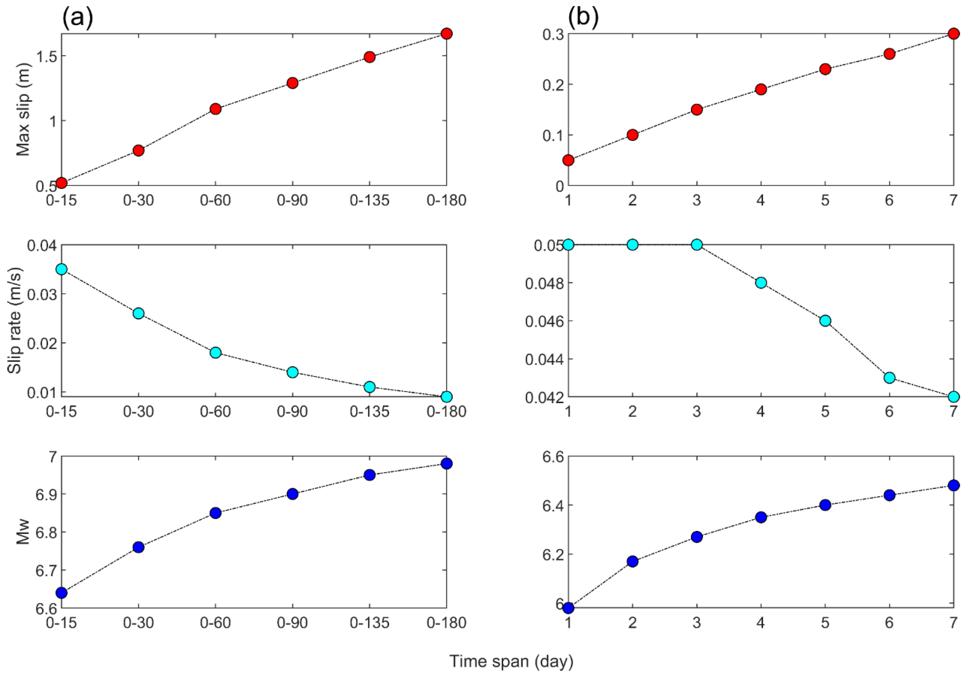
3.3. Spatio-Temporal Pattern Evolution of Afterslip
4. Discussion
4.1. Coulomb Stress Changes
4.2. Post-Seismic Fault Activity Properties
5. Conclusions
Author Contributions
Funding
Data Availability Statement
Acknowledgments
Conflicts of Interest
References
- Ishikawa, Y.; Bai, L. The 2024 Mj 7.6 Noto Peninsula, Japan earthquake caused by the fluid flow in the crust. Earthq. Res. Adv. 2024, 4, 100292. [Google Scholar] [CrossRef]
- Liu, Y.; Wu, Z.; Zhang, Y.; Yin, X. Tracing the pace of an approaching ‘seismic dragon king’: Additional evidence for the Noto earthquake swarm and the 2024 Mw 7.5 Noto earthquake. Earthq. Res. Adv. 2024, 4, 100290. [Google Scholar] [CrossRef]
- Mizuno, C.; Wang, X.; Dang, J. A Fast Survey Report About Bridge Damages by the 2024 Noto Peninsula Earthquake. Earthq. Res. Adv. 2024, 100312, accepted. [Google Scholar] [CrossRef]
- Kutschera, F.; Jia, Z.; Oryan, B.; Wing Ching Wong, J.; Fan, W.; Gabriel, A.A. Rapid earthquake-tsunami modeling: The multi-event, multi-segment complexity of the 2024 Mw 7.5 Noto Peninsula Earthquake governs tsunami generation. EarthArXiv 2024. [Google Scholar] [CrossRef]
- Mizutani, A.; Adriano, B.; Mas, E.; Koshimura, S. Fault model of the 2024 Noto Peninsula earthquake based on aftershock, tsunami, and GNSS data. Research Square 2024. [Google Scholar] [CrossRef]
- Pakoksung, K.; Suppasri, A.; Imamura, F. Preliminary modeling and analysis of the Tsunami generated by the 2024 Noto Peninsula earthquake on 1 January: Wave characteristics in the Sea of Japan. Ocean. Eng. 2024, 307, 118172. [Google Scholar] [CrossRef]
- Taira, A. Tectonic evolution of the Japanese island arc system. Annu. Rev. Earth Planet. Sci. 2001, 29, 109–134. [Google Scholar] [CrossRef]
- Hubbard, J.; Bradley, K. Tectonics of the January 1, 2024 M7.5 Earthquake in Japan: Exploring Earthquakes on Japan’s Western Coast. Earthquake Insights 2024. Available online: https://earthquakeinsights.substack.com/p/tectonics-of-the-january-1-2024-m75 (accessed on 15 August 2024).
- Yoshida, K.; Uchida, N.; Matsumoto, Y.; Orimo, M.; Okada, T.; Hirahara, S.; Kimura, S.; Hino, R. Updip fluid flow in the crust of the northeastern Noto Peninsula, Japan, triggered the 2023 Mw 6.2 Suzu earthquake during swarm activity. Geophys. Res. Lett. 2023, 50, e2023GL106023. [Google Scholar] [CrossRef]
- Shelly, D.R. Examining the connections between earthquake swarms, crustal fluids, and large earthquakes in the context of the 2020-2024 Noto Peninsula, Japan, earthquake sequence. Geophys. Res. Lett. 2024, 51, e2023GL107897. [Google Scholar] [CrossRef]
- Kato, A. Implications of fault-valve behavior from immediate aftershocks following the 2023 Mj 6.5 earthquake beneath the Noto Peninsula, central Japan. Geophys. Res. Lett. 2024, 51, e2023GL106444. [Google Scholar] [CrossRef]
- Fujii, Y.; Satake, K. Slip distribution of the 2024 Noto Peninsula earthquake (MJMA 7.6) estimated from tsunami waveforms and GNSS data. Earth Planets Space 2024, 76, 44. [Google Scholar] [CrossRef]
- Ma, Z.; Zeng, H.; Luo, H.; Liu, Z.; Jiang, Y.; Aoki, Y.; Wang, W.; Itoh, Y.; Lyu, M.; Cui, Y.; et al. Slow rupture in a fluid-rich fault zone initiated the 2024 M w 7.5 Noto earthquake. Science 2024, 385, 866–871. [Google Scholar] [CrossRef]
- Yang, S.; Sang, C.; Hu, Y.; Wang, K. Coseismic and early postseismic deformation of the 2024 Mw 7.45 Noto Peninsula earthquake. Geophys. Res. Lett. 2024, 51, e2024GL108843. [Google Scholar] [CrossRef]
- Nakajima, J. Crustal structure beneath earthquake swarm in the Noto peninsula, Japan. Earth Planets Space 2022, 74, 160. [Google Scholar] [CrossRef]
- Amezawa, Y.; Hiramatsu, Y.; Miyakawa, A.; Imanishi, K.; Otsubo, M. Long-living earthquake swarm and intermittent seismicity in the northeastern tip of the Noto Peninsula, Japan. Geophys. Res. Lett. 2023, 50, e2022GL102670. [Google Scholar] [CrossRef]
- Nishimura, T.; Hiramatsu, Y.; Ohta, Y. Episodic transient deformation revealed by the analysis of multiple GNSS networks in the Noto Peninsula, central Japan. Sci. Rep. 2023, 13, 8381. [Google Scholar] [CrossRef]
- Toda, S.; Stein, R.S. Intense seismic swarm punctuated by a magnitude 7.5 Japan shock. Temblor 2024. [Google Scholar] [CrossRef]
- Golriz, D.; Bock, Y.; Xu, X. Defining the coseismic phase of the crustal deformation cycle with seismogeodesy. J. Geophys. Res. Solid Earth 2021, 126, e2021JB022002. [Google Scholar] [CrossRef]
- Golriz, D.; Hirshorn, B.; Bock, Y.; Weinstein, S.; Weiss, J.R. Real-time seismogeodetic earthquake magnitude estimates for local tsunami warnings. J. Geophys. Res. Solid Earth 2023, 128, e2022JB025555. [Google Scholar] [CrossRef]
- Liu, K.; Geng, J.; Wen, Y.; Ortega-Culaciati, F.; Comte, D. Very early postseismic deformation following the 2015 Mw 8.3 Illapel earthquake, Chile revealed from kinematic GPS. Geophys. Res. Lett. 2022, 49, e2022GL098526. [Google Scholar] [CrossRef]
- Twardzik, C.; Vergnolle, M.; Sladen, A.; Avallone, A. Unravelling the contribution of early postseismic deformation using sub-daily GNSS positioning. Sci. Rep. 2019, 9, 1175. [Google Scholar] [CrossRef] [PubMed]
- Tsang, L.L.; Vergnolle, M.; Twardzik, C.; Sladen, A.; Nocquet, J.-M.; Rolandone, F.; Agurto-Detzel, H.; Cavalié, O.; Jarrin, P.; Mothes, P. Imaging rapid early afterslip of the 2016 Pedernales earthquake, Ecuador. Earth Planet. Sci. Lett. 2019, 524, 115724. [Google Scholar] [CrossRef]
- Xiang, Y.; Bian, Y.; Liu, J.; Xing, Y. Insights into very early afterslip associated with the 2021 M 8.2 Chignik, Alaska earthquake using subdaily GNSS solutions. Remote Sens. 2023, 15, 5469. [Google Scholar] [CrossRef]
- Zhao, B.; Du, R.; Zhang, R.; Tan, K.; Qiao, X.; Huang, Y.; Zhang, C. Co-seismic displacements associated with the 2015 Nepal Mw7.9 earthquake and Mw7.3 aftershock constrained by global positioning system measurements. Chin. Sci. Bull. 2015, 60, 2758–2764. (In Chinese) [Google Scholar]
- Zhao, B.; Yong, H.; Zhang, C.; Wei, W.; Kai, T.; Du, R. Crustal deformation on the Chinese mainland during 1998–2004 based on GPS data. Geod. Geodyn. 2015, 6, 7–15. [Google Scholar] [CrossRef]
- Wei, H.H.; Yu, T.N.; Tu, J.S.; Ke, F.Y. Detection and Evaluation of Flood Inundation Using CYGNSS Data during Extreme Precipitation in 2022 in Guangdong Province, China. Remote Sens. 2023, 15, 297. [Google Scholar] [CrossRef]
- Wei, H.H.; He, X.F.; Feng, Y.M.; Jin, S.G.; Shen, F. Snow depth estimation on slopes using GPS-Interferometirc reflectometry. Sensors 2019, 19, 4994. [Google Scholar] [CrossRef]
- Wei, H.; Yang, X.; Pan, Y.; Shen, F. GNSS-IR Soil Moisture Inversion Derived from Multi-GNSS and Multi-Frequency Data Accounting for Vegetation Effects. Remote Sens. 2023, 15, 5381. [Google Scholar] [CrossRef]
- Jiang, Z.S.; Yuan, L.; Huang, D.; Yang, Z.; Chen, W. Postseismic deformation associated with the 2008 Mw 7.9 Wenchuan earthquake, China: Constraining fault geometry and investigating a detailed spatial distribution of afterslip. J. Geodyn. 2017, 112, 12–21. [Google Scholar] [CrossRef]
- Jiang, Z.S.; Yuan, L.; Huang, D.; Yang, Z.; Hassan, A. Postseismic deformation associated with the 2015 Mw7.8 Gorkha earthquake, Nepal: Investigating ongoing afterslip and constraining crustal rheology. J. Asian Earth Sci. 2018, 156, 1–10. [Google Scholar] [CrossRef]
- Jiang, Z.S.; Huang, D.; Yuan, L.; Hassan, A.; Zhang, L.; Yang, Z. Coseismic and postseismic deformation associated with the 2016 Mw 7.8 Kaikoura earthquake, New Zealand: Fault movement investigation and seismic hazard analysis. Earth Planets Space 2018, 70, 62. [Google Scholar] [CrossRef]
- Xiang, Y.; Yue, J.; Wang, H.; Chen, Y. GNSS imaging coseismic and postseismic slip associated with the 2021 M 8.2 Chignik, Alaska earthquake. Tectonophysics 2024, 876, 230273. [Google Scholar] [CrossRef]
- Okada, Y. Surface deformation due to shear and tensile faults in a half-space. Bull. Seismol. Soc. Am. 1985, 75, 1135–1154. [Google Scholar] [CrossRef]
- Wang, R.; Diao, F.; Hoechner, A. SDM—A geodetic inversion code incorporating with layered crust structure and curved fault geometry. Proc. EGU Gen. Assem. 2013, 15, EGU2013–2411–1. [Google Scholar]
- Diao, F.; Xiong, X.; Wang, R.; Zheng, Y.; Walter, T.R.; Weng, H.; Li, J. Overlapping post-seismic deformation processes: Afterslip and viscoelastic relaxation following the 2011 Mw 9.0 Tohoku (Japan) earthquake. Geophys. J. Int. 2014, 196, 218–229. [Google Scholar] [CrossRef]
- Ji, C.; Wald, D.J.; Helmberger, D.V. Source description of the 1999 Hector Mine, California, earthquake, part I: Wavelet domain inversion theory and resolution analysis. Bull. Seismol. Soc. Am. 2002, 92, 1192–1207. [Google Scholar] [CrossRef]
- Wang, R.; Martín, F.L.; Roth, F. Computation of deformation induced by earthquakes in a multi-layered elastic crust—FORTRAN programs EDGRN/ EDCMP. Comput. Geosci. 2003, 29, 195–207. [Google Scholar] [CrossRef]
- Steacy, S. Introduction to special section: Stress transfer, earthquake triggering, and time-dependent seismic hazard. J. Geophys. Res. Solid Earth 2005, 110, B05S01. [Google Scholar] [CrossRef]
- Freed, A.M. Earthquake triggering by static, dynamic, and postseismic stress transfer. Annu. Rev. Earth Planet. Sci. 2005, 33, 335–367. [Google Scholar] [CrossRef]
- Stein, R.S. The role of stress transfer in earthquake occurrence. Nature 1999, 402, 605–609. [Google Scholar] [CrossRef]
- Lin, J.; Stein, R.S. Stress triggering in thrust and subduction earthquakes, and stress interaction between the southern San Andreas and nearby thrust and strikeslip faults. J. Geophys. Res. Solid Earth 2004, 109, B02303. [Google Scholar] [CrossRef]
- Toda, S.; Stein, R.S.; Richards-Dinger, K.; Bozkurt, S.B. Forecasting the evolution of seismicity in southern California: Animations built on earthquake stress transfer. J. Geophys. Res. Solid Earth 2005, 110, B03415. [Google Scholar] [CrossRef]
- Ozawa, S.; Yarai, H.; Tobita, M.; Une, H.; Nishimura, T. Crustal deformation associated with the Noto Hanto Earthquake in 2007 in Japan. Earth Planets Space 2008, 60, 95–98. [Google Scholar] [CrossRef]
- Toda, S. Coulomb stresses imparted by the 25 March 2007 M w = 6.6 Noto-Hanto, Japan, earthquake explain its ‘butterfly’distribution of aftershocks and suggest a heightened seismic hazard. Earth Planets Space 2008, 60, 1041–1046. [Google Scholar] [CrossRef]
- Feigl, K.L.; Thatcher, W. Geodetic observations of post-seismic transients in the context of the earthquake deformation cycle. C. R. Geosci. 2006, 338, 1012–1028. [Google Scholar] [CrossRef]
- Ozawa, S.; Nishimura, T.; Munekane, H.; Suito, H.; Kobayashi, T.; Tobita, M.; Imakiire, T. Preceding, coseismic, and postseismic slips of the 2011 Tohoku earthquake, Japan. J. Geophys. Res. Solid Earth 2012, 117, B07404. [Google Scholar] [CrossRef]
- Bedford, J.; Moreno, M.; Baez, J.C.; Lange, D.; Tilmann, F.; Rosenau, M.; Vigny, C. A high-resolution, time-variable afterslip model for the 2010 Maule Mw= 8.8, Chile megathrust earthquake. Earth Planet. Sci. Lett. 2013, 383, 26–36. [Google Scholar] [CrossRef]
- Perfettini, H.; Avouac, J.P. The seismic cycle in the area of the 2011 Mw 9.0 Tohoku-Oki earthquake. J. Geophys. Res. Solid Earth 2014, 119, 4469–4515. [Google Scholar] [CrossRef]
- Hsu, Y.J.; Simons, M.; Avouac, J.P.; Galetzka, J.; Sieh, K.; Chlieh, M.; Bock, Y. Frictional afterslip following the 2005 Nias-Simeulue earthquake, Sumatra. Science 2006, 312, 1921–1926. [Google Scholar] [CrossRef]
- Freed, A.M. Afterslip (and only afterslip) following the 2004 Parkfield, California earthquake. Geophys. Res. Lett. 2007, 34, L06312. [Google Scholar] [CrossRef]
- Wang, R.; Lorenzo-Martín, F.; Roth, F. PSGRN/PSCMP—A new code for calculating co-and post-seismic deformation, geoid and gravity changes based on the viscoelastic-gravitational dislocation theory. Comput. Geosci. 2006, 32, 527–541. [Google Scholar] [CrossRef]


| Depth (km) | P_vel (km/s) | S_vel (km/s) | Dens. (g/cm3) | Qp | Qs |
|---|---|---|---|---|---|
| 0.000 | 2.76 | 0.69 | 1.84 | 1200.0 | 600.0 |
| 0.376 | 6.18 | 3.59 | 2.68 | 1200.0 | 600.0 |
| 9.745 | 6.73 | 3.68 | 2.75 | 1200.0 | 600.0 |
| 20.291 | 6.96 | 3.83 | 2.81 | 1200.0 | 600.0 |
| 33.572 | 8.08 | 4.47 | 3.38 | 1200.0 | 600.0 |
| 229.572 | 8.59 | 4.66 | 3.45 | 360.0 | 140.0 |
| Site | Lon. | Lat. | Post-Seismic Deformations (mm) | Site | Lon. | Lat. | Post-Seismic Deformations (mm) | ||||
|---|---|---|---|---|---|---|---|---|---|---|---|
| North | East | Up | North | East | Up | ||||||
| G109 | 138.28 | 37.81 | 10.83 | −12.98 | 2.91 | J266 | 137.87 | 36.70 | 10.42 | −5.21 | 0.76 |
| G110 | 138.50 | 37.35 | 10.15 | −14.39 | 9.65 | J267 | 138.24 | 36.66 | 10.27 | −9.51 | 9.12 |
| G158 | 136.77 | 37.00 | 6.12 | −15.42 | −16.31 | J448 | 132.99 | 32.99 | 0.23 | 2.50 | 4.85 |
| G207 | 137.22 | 36.76 | 13.22 | −15.66 | 8.65 | J567 | 138.51 | 37.34 | 10.30 | −14.16 | 13.19 |
| I002 | 140.17 | 36.26 | 1.82 | −3.97 | −1.79 | J569 | 138.24 | 37.05 | 8.42 | −19.96 | 3.97 |
| I028 | 139.46 | 35.52 | 2.91 | −1.32 | −1.26 | J570 | 137.89 | 36.95 | 17.63 | −20.72 | 12.92 |
| I064 | 138.97 | 35.62 | 12.27 | −0.17 | −0.38 | J572 | 137.36 | 36.73 | 15.31 | −14.16 | 9.48 |
| J050 | 138.98 | 37.89 | 2.91 | −8.06 | 4.09 | J573 | 137.03 | 36.64 | 7.33 | −10.92 | −0.26 |
| J051 | 138.57 | 37.39 | 9.71 | −11.74 | 10.92 | J574 | 137.13 | 37.30 | 19.90 | −30.29 | −28.85 |
| J052 | 137.48 | 36.92 | 23.52 | −24.61 | 22.43 | J575 | 136.71 | 37.15 | 3.47 | −6.00 | −12.07 |
| J053 | 136.88 | 37.38 | 4.82 | −3.03 | −59.12 | J576 | 136.99 | 37.12 | 14.16 | −16.43 | −29.44 |
| J235 | 138.27 | 37.81 | 10.30 | −11.24 | 0.61 | J807 | 138.77 | 37.49 | 6.15 | −13.39 | 11.13 |
| J241 | 138.33 | 37.23 | 13.45 | −17.28 | 13.42 | J962 | 138.63 | 37.21 | 7.95 | −14.42 | 15.22 |
| J243 | 138.10 | 37.16 | 21.67 | −19.34 | 19.10 | J964 | 138.45 | 37.10 | 11.60 | −15.54 | 15.75 |
| J244 | 138.60 | 37.07 | 7.24 | −14.51 | 7.59 | J966 | 137.02 | 36.91 | 15.39 | −18.78 | −3.56 |
| J245 | 137.87 | 37.04 | 22.87 | −21.20 | 17.87 | J967 | 137.55 | 36.86 | 19.87 | −21.52 | 7.80 |
| J247 | 138.19 | 36.86 | 13.36 | −19.37 | 4.85 | J968 | 137.15 | 36.75 | 13.27 | −15.66 | −2.79 |
| J248 | 136.99 | 36.74 | 10.54 | −12.95 | −4.26 | J970 | 137.23 | 36.47 | 8.03 | −6.68 | −6.24 |
| J250 | 137.43 | 36.57 | 12.57 | −6.89 | 8.21 | J972 | 136.90 | 37.22 | 10.60 | −24.05 | −36.36 |
| J253 | 137.27 | 37.44 | 30.59 | −26.97 | −67.75 | R006 | 138.05 | 36.45 | 10.18 | −3.35 | 12.07 |
| J265 | 138.43 | 36.80 | 9.01 | −11.68 | 7.74 | R015 | 137.72 | 36.55 | 12.42 | −11.30 | 9.62 |
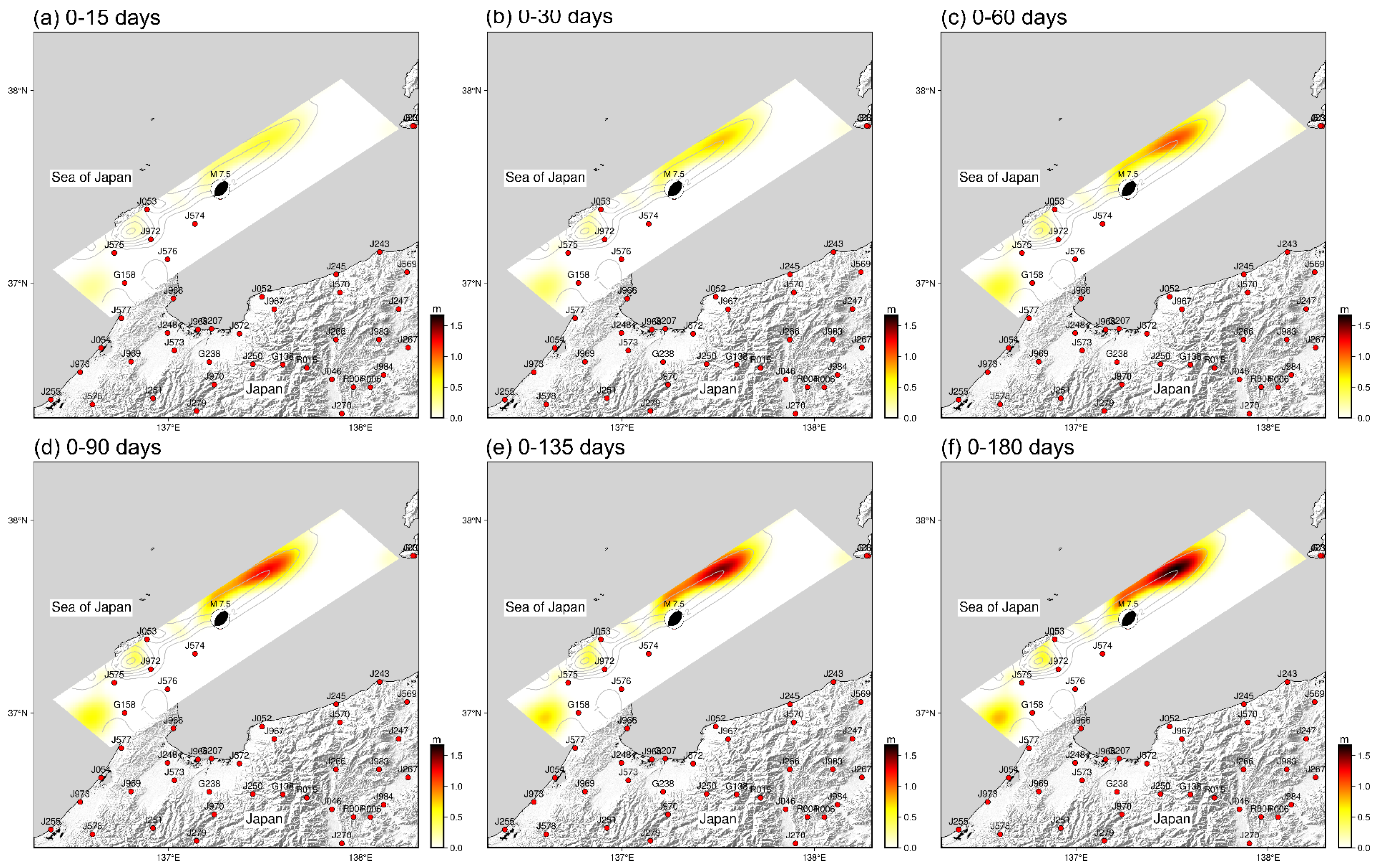
| Time Period (days) | Mean Slip (m) | Mean Stress Drop (MPa) | Maximum Slip | Maximum Slip Rate (m/day) | Mw | |
|---|---|---|---|---|---|---|
| Value (m) | Depth (km) | |||||
| 0–15 | 0.04 | 0.46 | 0.52 | 5.43 | 0.035 | 6.64 |
| 0–30 | 0.06 | 0.69 | 0.77 | 5.43 | 0.026 | 6.72 |
| 0–60 | 0.09 | 0.99 | 1.09 | 5.43 | 0.018 | 6.76 |
| 0–90 | 0.11 | 1.16 | 1.29 | 5.43 | 0.014 | 6.90 |
| 0–135 | 0.12 | 1.34 | 1.49 | 5.43 | 0.011 | 6.95 |
| 0–180 | 0.14 | 1.50 | 1.67 | 5.43 | 0.009 | 6.98 |
Disclaimer/Publisher’s Note: The statements, opinions and data contained in all publications are solely those of the individual author(s) and contributor(s) and not of MDPI and/or the editor(s). MDPI and/or the editor(s) disclaim responsibility for any injury to people or property resulting from any ideas, methods, instructions or products referred to in the content. |
© 2024 by the authors. Licensee MDPI, Basel, Switzerland. This article is an open access article distributed under the terms and conditions of the Creative Commons Attribution (CC BY) license (https://creativecommons.org/licenses/by/4.0/).
Share and Cite
Xiang, Y.; Qin, M.; Chen, Y.; Xing, Y.; Bian, Y. Co-Seismic and Post-Seismic Slip Properties Associated with the 2024 M 7.5 Noto Peninsula, Japan Earthquake Determined by GNSS Observations. Remote Sens. 2024, 16, 4057. https://doi.org/10.3390/rs16214057
Xiang Y, Qin M, Chen Y, Xing Y, Bian Y. Co-Seismic and Post-Seismic Slip Properties Associated with the 2024 M 7.5 Noto Peninsula, Japan Earthquake Determined by GNSS Observations. Remote Sensing. 2024; 16(21):4057. https://doi.org/10.3390/rs16214057
Chicago/Turabian StyleXiang, Yunfei, Ming Qin, Yuanyuan Chen, Yin Xing, and Yankai Bian. 2024. "Co-Seismic and Post-Seismic Slip Properties Associated with the 2024 M 7.5 Noto Peninsula, Japan Earthquake Determined by GNSS Observations" Remote Sensing 16, no. 21: 4057. https://doi.org/10.3390/rs16214057
APA StyleXiang, Y., Qin, M., Chen, Y., Xing, Y., & Bian, Y. (2024). Co-Seismic and Post-Seismic Slip Properties Associated with the 2024 M 7.5 Noto Peninsula, Japan Earthquake Determined by GNSS Observations. Remote Sensing, 16(21), 4057. https://doi.org/10.3390/rs16214057