Abstract
This research presents a novel fuzzy-logic-based algorithm aimed at detecting and removing interference lines from Micro Rain Radar (MRR-2) data. Interference lines, which are non-meteorological echoes with unknown origins, can severely obscure meteorological signals. Leveraging an understanding of interference line characteristics, such as temporal continuity, we identified and utilized eight key variables to distinguish interference lines from meteorological signals. These variables include radar moments, Doppler spectrum peaks, and the spatial/temporal continuity of Doppler velocity. The algorithm was developed and validated using data from MRR installations at three sites (Seoul, Suwon, and Incheon) in South Korea, from June to September 2021–2023. While there is a slight tendency to eliminate some weak precipitation, results indicate that the algorithm effectively removes interference lines while preserving the majority of genuine precipitation signals, even in complex scenarios where both interference and precipitation signals are present. The developed software, written in Python 3 and available as open-source, outputs in NetCDF4 format, with customizable parameters for user flexibility. This tool offers a significant contribution to the field, facilitating the accurate interpretation of MRR-2 data contaminated by interference.
1. Introduction
The Micro Rain Radar (MRR-2), a vertically pointing radar, has been widely employed in field campaigns to provide a comprehensive and in-depth understanding of specific meteorological phenomena. The MRR-2, developed by Metek, Germany, is a K-band (24.23 GHz) frequency-modulated continuous-wave (FMCW) radar. Its compactness, low cost, and stable observational capabilities offer significant benefits when deploying multiple MRRs at different geographical locations, facilitating a spatial understanding of the vertical structure of precipitation [1,2,3,4,5].
To ensure the high data quality of MRR-2, post-processing algorithms were proposed to better determine noise levels from the Doppler spectrum and to improve the Doppler de-aliasing. Maahn and Kollias [6] (hereafter, MK12) proposed a widely recognized post-processing algorithm that improves sensitivity compared to the manufacturer’s algorithm and introduces Doppler de-aliasing for snow and light rain events. Similarly, Garcia-Benadi et al. [7] introduced an algorithm that enhances sensitivity and Doppler de-aliasing, while also providing precipitation type classification.
In this paper, what we refer to as “interference lines” are artificial, non-meteorological echoes that appear continuously over time at arbitrary altitudes [8]. This signal could potentially be an internal signal [8] or caused by sidelobes, but the exact origin remains uncertain. These signals were not fully considered in the earlier post-processing algorithms, and, to the best of our knowledge, no algorithm has yet been proposed to detect and remove such signals specifically for the MRR-2. From long-term observational data collected from various MRR-2 instruments, we identified several characteristics of these interference lines: (1) They predominantly occur at higher range gates, rather than in the lower atmospheric layers. (2) They persist in 1–3 consecutive range gates for several hours to several days before disappearing. (3) Multiple interference lines can appear simultaneously across different range gates. (4) Although interference lines tend to reappear in the same range gate where they initially occurred, they are likely to appear at different altitudes under certain environmental changes (such as a change in power source or site relocation). (5) These lines appear in all fields. (6) The values of reflectivity, Doppler velocity, and other parameters for these lines are not constant over time and differ between lines. These characteristics suggest that detecting and eliminating these lines are not straightforward using a simple approach. In particular, their variability in range gates, unpredictable and inconsistent occurrence over time, and fluctuations in values make them challenging to detect.
The interference lines in the MRR-PRO, the successor to the MRR-2 [9], were successfully identified and removed by Ferrone et al. [8]. They accomplished this by detecting the signals corresponding to these interference lines from the raw Doppler spectrum and removing them through spectrum reconstruction. Their algorithm was specifically developed for the MRR-PRO and can be effectively utilized by the community using this instrument [10,11,12]. It is noteworthy to mention that the final products of MRR2 and MRR-PRO differ in terms of when signal quality is determined and applied. It is also uncertain whether the interference lines detected in MRR2 are the same as those found in MRR-PRO. Extensive modifications to the code will also likely be required due to different output formats. While the MRR-PRO, as a relatively recent instrument, offers enhanced sensitivity and greater flexibility in configuration, the MRR-2, which has been utilized in research for decades, remains actively used in field campaigns [7,13,14,15]. Therefore, we believe the development of the MRR-2-specific interference line removal algorithm will be beneficial to the scientific community.
In this study, we developed a more straightforward algorithm utilizing fuzzy logic. The primary motivation behind our approach was to ensure that these interference lines do not interfere with the analysis of precipitation characteristics using the MRR-2 dataset. Consequently, we concentrated on detecting and eliminating these interference lines. In cases where precipitation and interference lines coexisted, our objective was to eliminate any data affected by the interference lines.
Our paper is organized as follows. Section 2 provides a description of the MRR-2 data used and a detailed explanation of the algorithm. Section 3 assesses the performance of the developed algorithm by applying it to MRR-2 data. Section 4 discusses the application of the algorithm and provides recommendations along with the conclusions of the study.
2. Data and Algorithm Description
In this study, data were obtained from MRRs installed at three locations: Incheon (ICN: 37.4777°N, 126.6249°E), Suwon (SWN: 37.2575°N, 126.9830°E), and Seoul (SEL: 37.5714°N, 126.9658°E). The dataset covers the period from June to September across three years (2021–2023). All days were observed normally at all sites, except for three days of missing data at SEL. For all three sites, the MRRs were configured with a vertical resolution of 150 m.
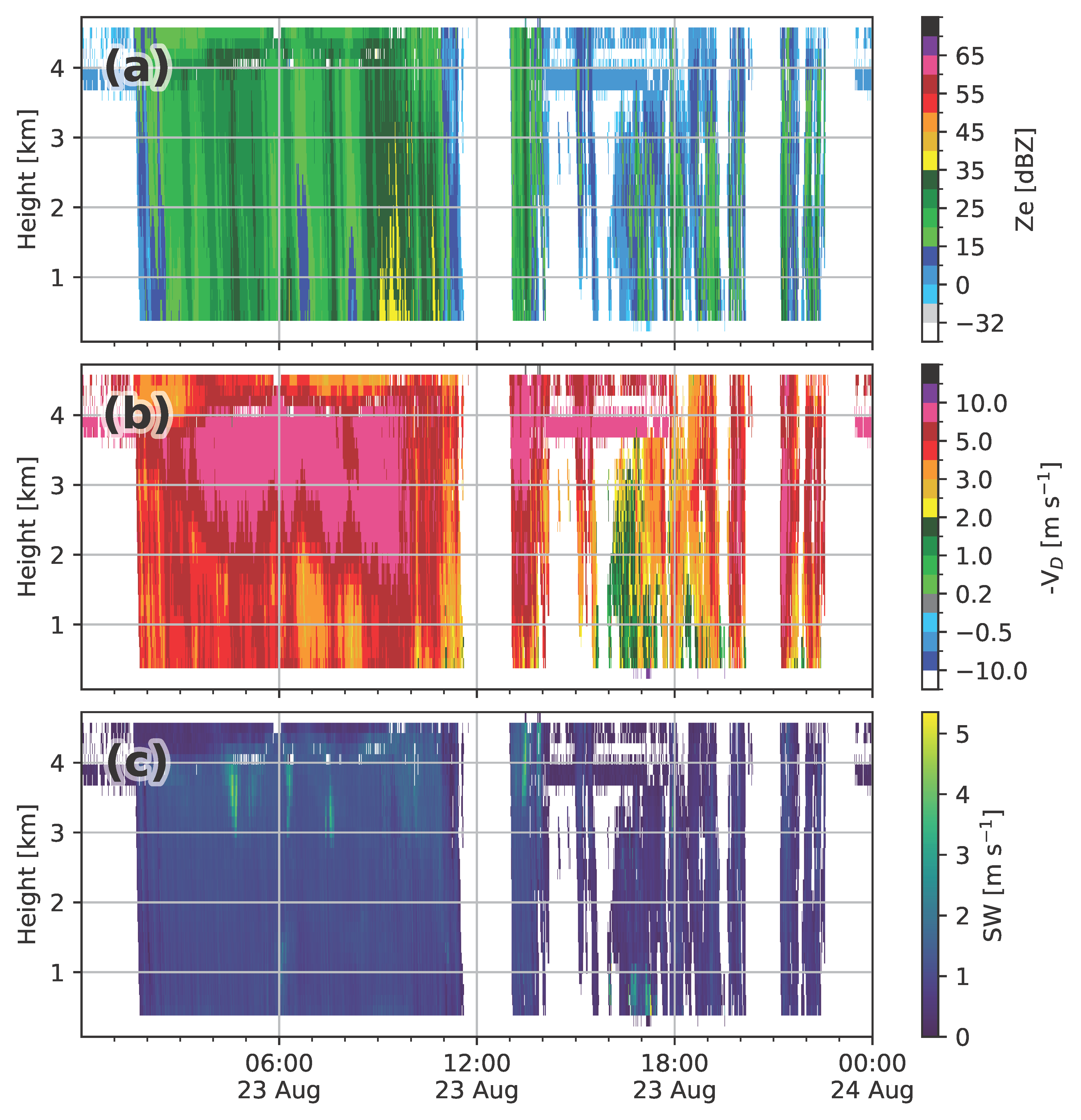
Figure 1 shows an example of significant interference lines observed at the ICN site. The data show contamination by interference lines across seven range gates, from approximately 3.7 km to 4.7 km altitude. This interference is clearly visible until 02 UTC, just before the precipitation begins. It disappears near 12 UTC, reappears between 14 and 18 UTC, and then reemerges after 23 UTC. The interference lines consistently appear at the same heights and times in all variables, with variabilities in reflectivity and Doppler velocity values. The following section details the algorithm developed to detect and remove these signals.

Figure 1.
Time–height diagrams of MRR-2 data for the ICN site on 23 August 2021: (a) reflectivity, (b) Doppler velocity, and (c) spectrum width.
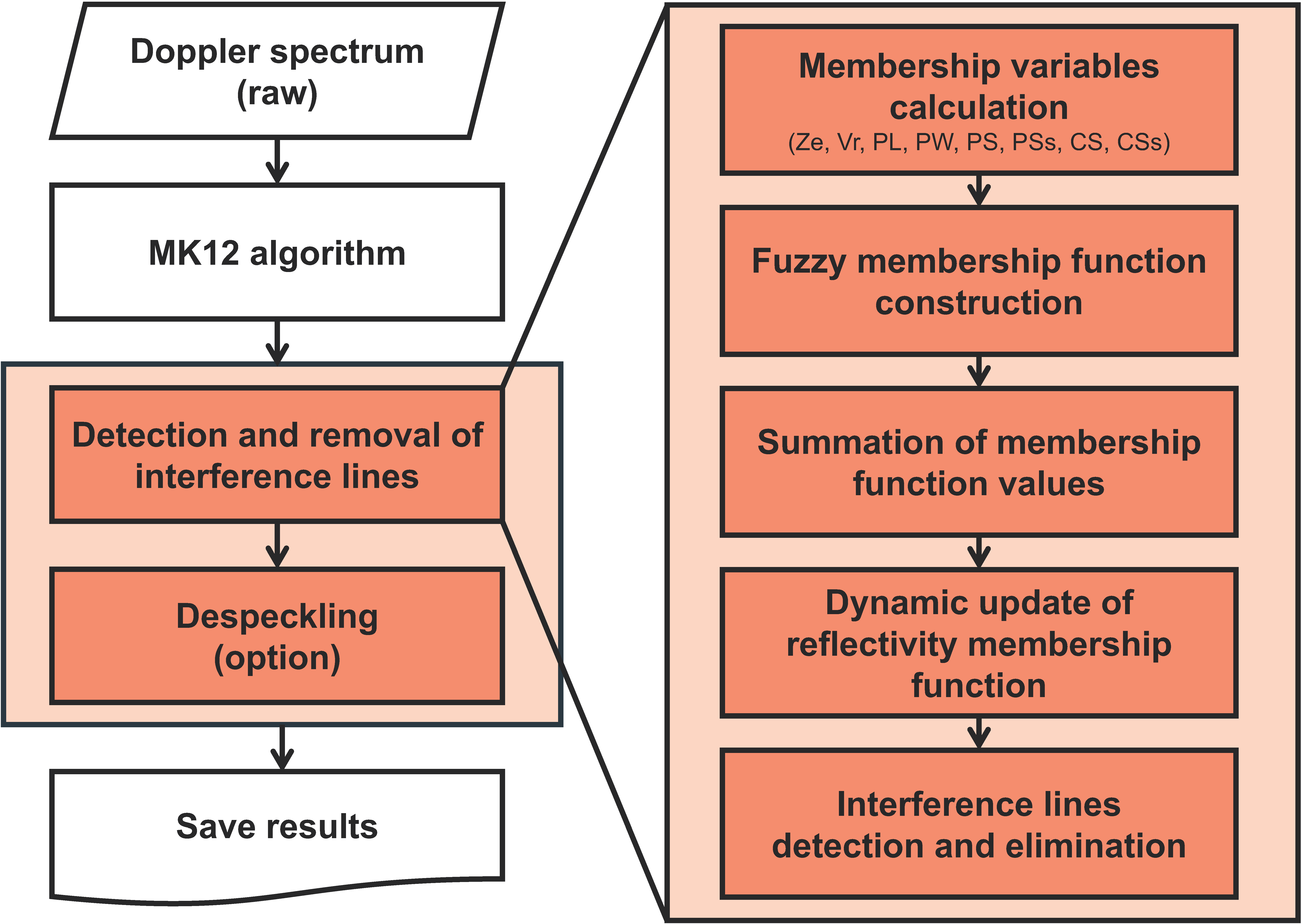
The algorithm flow from the raw Doppler spectrum provided by MRR-2 to the final result is illustrated in Figure 2. The process began with applying the MK12 algorithm to the raw data to estimate the noise level. Then, the MK12 algorithm extracted the properties of the spectrum peak (left and right boundaries, slope) and derived radar moments (reflectivity, Doppler velocity) from this peak. During this process, the raw spectrum data, initially recorded in 10 s intervals, were averaged and stored as 1 min outputs.
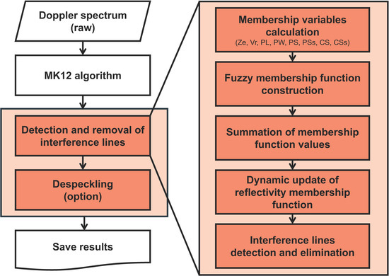
Figure 2.
A flow chart of the algorithm for detecting and removing interference lines in MRR-2 data.
Subsequently, the algorithm focused on detecting and removing interference lines using fuzzy logic. After thoroughly analyzing whether the output variables of the MK12 algorithm could effectively distinguish between interference lines and meteorological variables, we selected the fuzzy membership variables. These variables included two moment-related variables, four peak-related variables, and two spatiotemporal continuity variables of Doppler velocities. The following describes the detailed procedure for each step.
2.1. Membership Variables’ Calculation
Moment-related variables included reflectivity (Z) and Doppler velocity (Vr). Interference lines typically exhibit reflectivity values ranging from −5 to 20 dBZ and Doppler velocities between 4 and 9 m s−1. Peak-related variables consist of the peak left boundary (PL), peak width (PW), peak slope (PS), and smoothed peak slope (PSs). For interference lines, the PL generally starts at values above 4 m s−1, with a narrow spectrum width (usually less than 2 m s−1) and a steep slope (typically greater than 10). Doppler velocity spatiotemporal continuity-related variables include Doppler velocity spatial continuity (CS) and smoothed Doppler velocity spatial continuity (CSs). Interference lines typically show shallow vertical thickness in spatial continuity. The temporal continuity of CS was assessed using CSs. Calculations and window information for these variables are detailed in Table 1.

Table 1.
Description of fuzzy membership variables.
Our method was specifically developed for application to rain events. In the MK12 algorithm, de-aliasing was introduced to account for hydrometeors with small fall velocities (e.g., snow), which can be easily lifted by updrafts, occasionally resulting in positive (upward) Doppler velocities and Doppler aliasing. However, in our study, we decided to use variables where de-aliasing was not applied because it is not suitable for moderate to heavy rain events, particularly those with strong reflectivity in convective systems (MK12).
2.2. Fuzzy Membership Function Construction
Fuzzy membership functions for each characteristic variable were obtained using logistic regression with a sigmoid function, assigning the label 1 to interference lines and 0 to precipitation. Note that we employed logistic regression solely for the purpose of constructing fuzzy membership functions, specifically to identify the parameters a and b of the sigmoid function, rather than directly utilizing it to address a classification problem.
The labeling of interference lines and precipitation was based on pre-classified samples from time–height diagrams as determined by the authors. The dataset included samples from 23 August 2021 to 2 September 2021, from the ICN and SWN sites, comprising 38,648 samples of interference lines and 58,062 samples of precipitation. The SEL site was used to assess whether the algorithm performed effectively with an independent instrument at a different location. To ensure an equal number of samples for interference lines and precipitation, precipitation samples were randomly selected to match the number of interference line data points. The fuzzy membership function was defined as follows:
where represents the membership variable value and and are constant parameters. As detailed in Table 2, the parameters a and b for each membership variable were determined via logistic regression. For this analysis, we employed the LogisticRegression function from python scikit-learn (version 1.4.2), utilizing the default configuration with L2 regularization. Our loss function was as follows:
where y denotes the true label (1 for interference line and 0 for precipitation), p represents the predicted probability, is the regularization strength parameter (set to 1), denotes the weight for each parameter (also set to 1), N indicates the total number of samples, and M is the total number of parameters. Log loss values are also presented in Table 2, where smaller values indicate a better fit to the data. We further evaluated the fit using pseudo-R squared, which ranges from 0 (complete failure) to 1 (complete success). Values between 0.2 and 0.4 indicate a very good fit. Our results indicated that the membership functions generally represented the samples well.
Table 2.
Determined a, b parameters, log loss, and pseudo-R squared values of each membership variable.
Figure 3 shows the constructed membership functions corresponding to each variable. The variables with minimal overlap in interference lines and precipitation values (e.g., PL) were constructed with a steep slope in the membership function within the overlapping range. In contrast, variables with higher overlap (e.g., Vr) were constructed with a gentler slope.
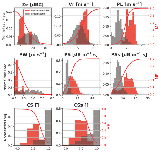
Figure 3.
Histograms of precipitation samples and interference lines for each membership variable, with the constructed membership function depicted by the red line on the secondary y-axis.
2.3. Summation of Membership Function Values
The membership function values for each characteristic variable were weighted and aggregated using a weighted sum, as follow:
where is the membership function for the variable and represents the weight for the i-th variable. The weight () for each characteristic variable is computed based on the cross-correlation coefficient between the sigmoid function of the logistic regression and the actual binomial probabilities (0 or 1) (Table 3). In other words, the weights were derived using the red line of the membership function in Figure 3 and the labeled data points (0 or 1), which are represented by a histogram.
Table 3.
The weight of each membership variable.
2.4. Dynamic Update of Reflectivity Membership Function
We observed that, while the fuzzy membership function described above generally performed well in detecting interference lines, there were occasional failures. The primary cause of these failures was the significant variability in the reflectivity of the interference lines, leading to discrepancies between the observed reflectivity values and the predefined membership function. In particular, when multiple interference lines appeared simultaneously, the algorithm struggled to detect if there was a large deviation in their reflectivity values. This finding led to the idea of introducing a dynamic updating process for the membership function specifically for reflectivity.
To update the membership function, we first classified data into interference line candidates and precipitation candidates based on the AGG values in Equation (2) and their altitude criteria. Interference line candidates were identified as data with an AGG of 0.5 or greater and a range gate index of 22 or higher (out of 32 indices, corresponding to higher altitudes). In contrast, precipitation candidates were defined by AGG values below 0.5 and range gate indices lower than 22. Similar to the initial construction of the membership function, the sample sizes for each candidate were equalized by randomly downsampling the larger set to match the smaller set. If an adequate number of samples was not available for either category (defined as fewer than 30 samples in this study), the dynamic update was not performed.
Upon identifying the candidates, the membership function was updated. Given that multiple modes were observed in the distribution due to differences in reflectivity among interference lines, we defined the membership function using a generalized bell shape that allowed for multiple peaks. The updated membership function is expressed in the following form:
where i indicates the peak index, which may correspond to one or more peaks, and the constants , , and are the shape parameters of the generalized bell-shaped function corresponding to each peak.
The find_peaks function from SciPy (version 1.9.1) was utilized to determine the number of peaks (Npeak), their widths, and their positions. The parameters for peak detection were set with a minimum height of 0.02 and a minimum distance of 10. Each detected peak was represented by a generalized bell-shaped function, where c was 0.6667 times the peak width, d was set to 3, and e corresponded to the peak position. These functions were summed for each peak, with any values exceeding 1 capped at 1 to update the reflectivity membership functions. The updated membership functions were then used to calculate the cross-correlation coefficient with the actual binomial probabilities (i.e., interference line and precipitation candidates), and the reflectivity weights were adjusted accordingly.
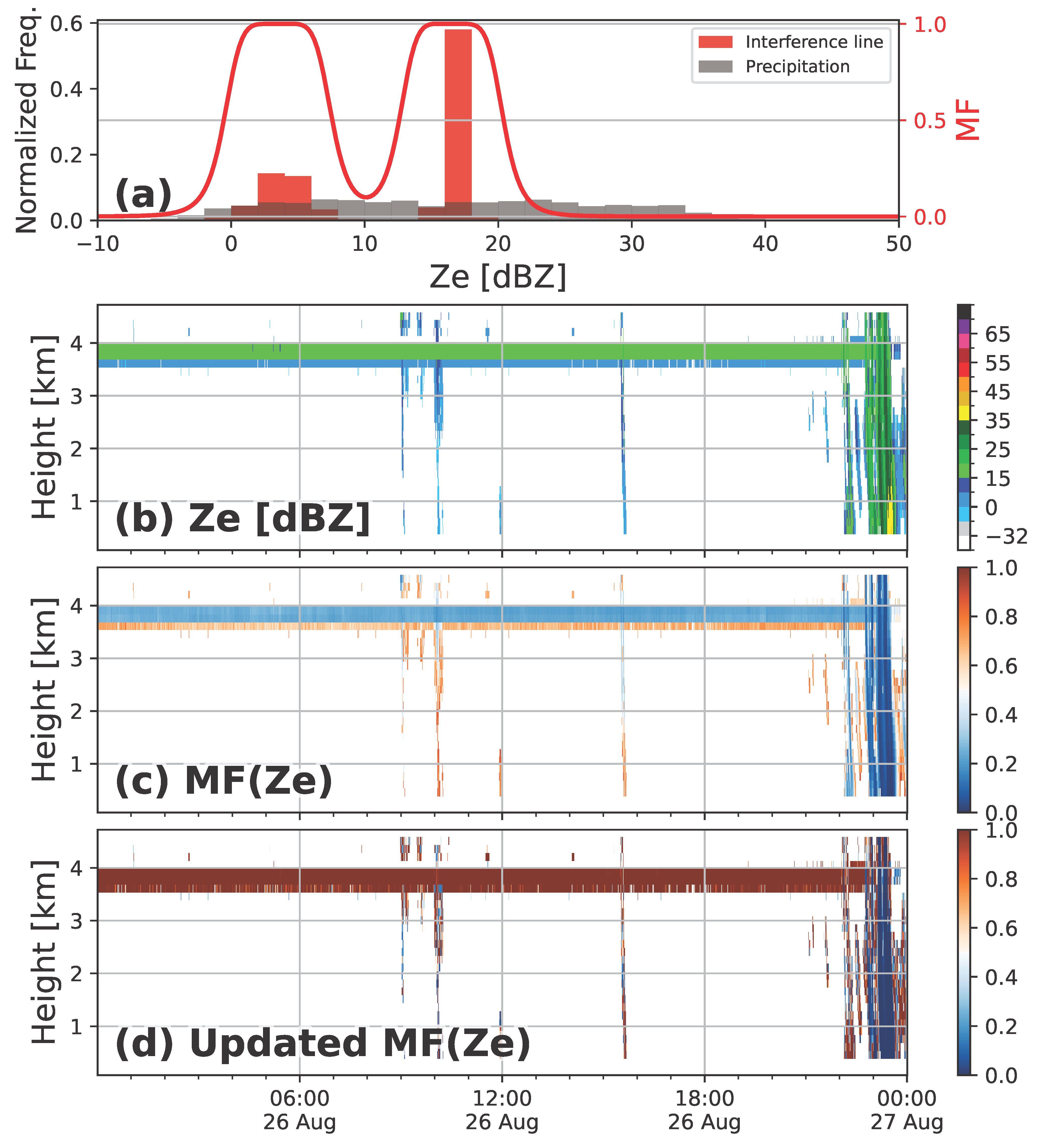
Figure 4 illustrates an example of updating the membership function using reflectivity from interference line candidates with two modes. During the period from 00–23 UTC, interference lines at altitudes between 3.5 km and 4 km displayed two modes in reflectivity: one in the range of 0–7 dBZ and another in the range of 15–20 dBZ. The initial fuzzy membership function, as constructed previously, yielded lower values for the higher reflectivity mode. This is evident in Figure 4b, where interference lines at 4 km altitude show values below 0.5, indicating that the reflectivity variable hindered the detection of interference lines. By updating the membership function to achieve higher values in both modes (Figure 4d), the results were significantly improved as the value approached 1 (Figure 4c).
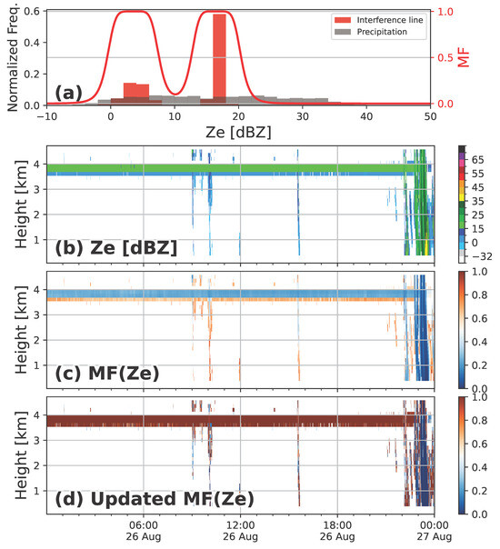
Figure 4.
(a) Similar to Figure 3 but showing interference line and precipitation candidate samples obtained from (b) and the updated reflectivity membership function. Time–height diagrams for the ICN site MRR-2 on 26 August 2021: (b) Ze, (c) MF(Ze), and (d) updated MF(Ze).
2.5. Interference Lines’ Detection and Elimination
If the reflectivity membership function and corresponding weights were updated, the AGG values were revised to reflect these updates. In cases where the sample size for candidates was insufficient (in our case, fewer than 30) and no update was made, previously determined AGG values were retained. Ultimately, an AGG value greater than 0.5 indicated a high likelihood of interference lines, and such instances were classified as interference lines.
2.6. Despeckling
Following the removal of interference lines, the algorithm optionally applied a despeckling procedure to further eliminate noise frequently observed in clear skies. Specifically, this process involved removing data points if the number of valid data points within a 33 (time altitude) sliding window was equal to or less than 1.
2.7. Open-Source Software
The software, developed in Python 3, is available as open-source on GitHub at https://github.com/Kwonil-Kim/MRR2_interference_line_removal (accessed on 15 October 2024). It provides flexibility by allowing users to adjust various parameters utilized by the algorithm. These include the option to perform despeckling, the AGG threshold for final detection, predefined fuzzy membership function parameters, weights, the minimum range gate for identifying interference line candidates, window sizes for membership variable calculations, and window size and thresholds for despeckling. The output is stored in NetCDF4 format, preserving the MK12 variable list and including additional membership function values for each variable and AGG value.
3. Results
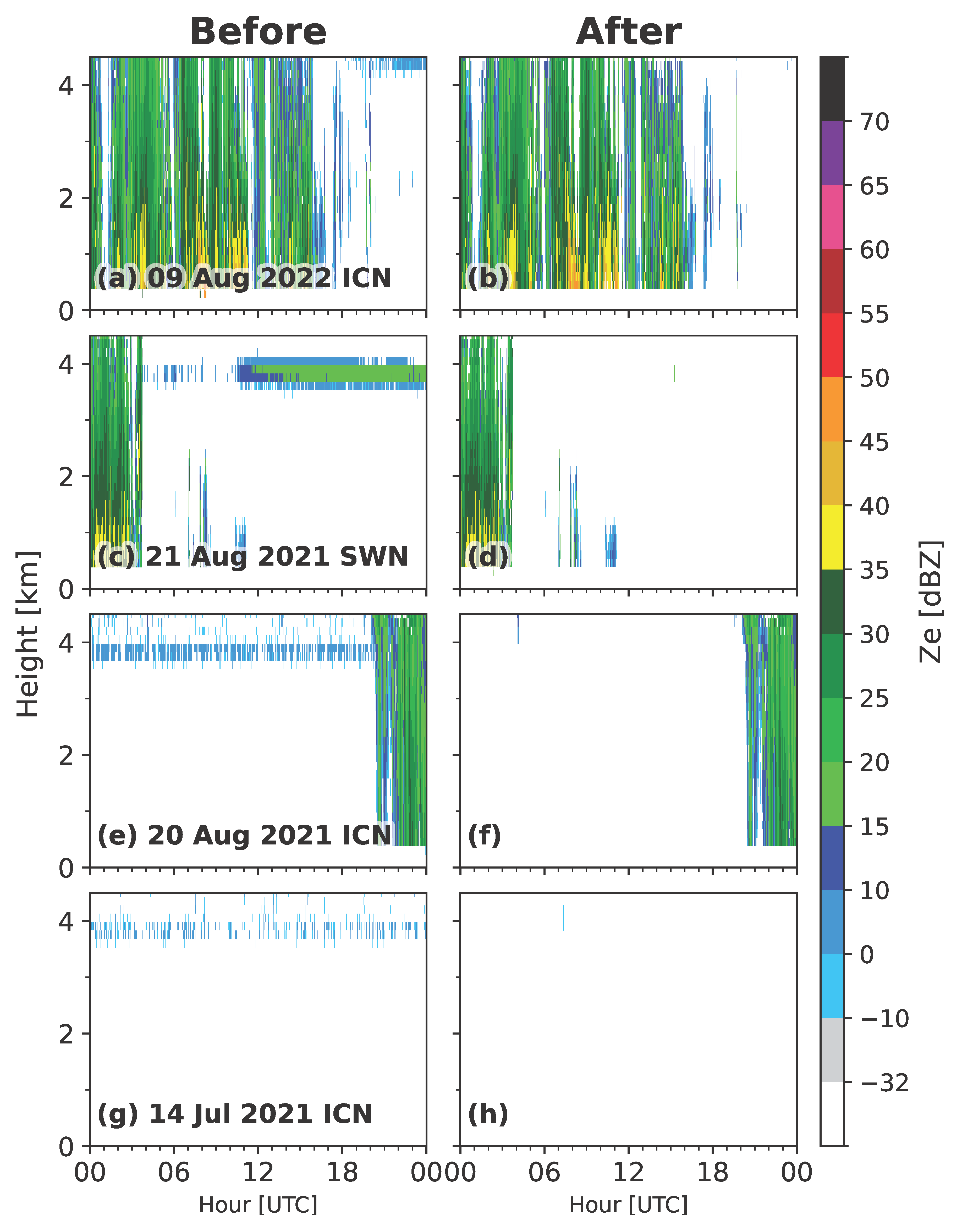
We assessed the performance of the developed algorithm by applying it to multiple instances where interference lines were observed. Figure 5 presents examples of three distinct rainfall events and one clear sky event. The rain event on 9 August 2022 at ICN (Figure 5a) was characterized by long precipitation durations of approximately 18 h, with interference lines appearing and disappearing multiple times. In contrast, the two rain events on 21 August 2021 at SWN (Figure 5c) and 20 August 2021 at ICN (Figure 5e) featured a shorter precipitation duration of less than 6 h, with interference lines being dominant throughout. The clear sky event on 14 July 2021 at ICN (Figure 5g) exhibited no meteorological echoes, with interference lines appearing intermittently for short durations throughout the day. Across all events, the interference lines were significant, extending over approximately seven range gates at altitudes above 3.5 km.

Figure 5.
Time–height diagrams of reflectivity for the ICN and SWN sites. From top to bottom, each row corresponds to 9 August 2021 (ICN); 21 August 2021 (SWN); 28 August 2021 (ICN); and 13 July 2021 (ICN). Each column represents the data before (denoted as “Before”, corresponding to the data after the MK12 algorithm) and after applying the algorithm (denoted as “After”).
Our algorithm successfully detected and removed these persistent interference lines along the time axis. Importantly, we highlight that, while the interference lines were eliminated, the precipitation echoes were preserved. For example, in Figure 5a, interference lines between 18 and 24 UTC were successfully removed. Even in challenging cases, such as those shown in Figure 5a between 13 and 16 UTC, where interference lines were almost indistinguishable from precipitation echoes from the reflectivity field, the algorithm performed well by utilizing the other fuzzy membership variables. As shown in Figure 5c,d, the algorithm detected interference lines even when they appeared across multiple altitudes with a broad reflectivity range of 0–20 dBZ. Moreover, within the same event, the algorithm was able to detect them when they were temporally discontinuous and fragmented. When interference lines persisted throughout the event (Figure 5e), the algorithm also demonstrated good performance. Particularly in the clear sky event (Figure 5g), all non-meteorological echoes were successfully removed.
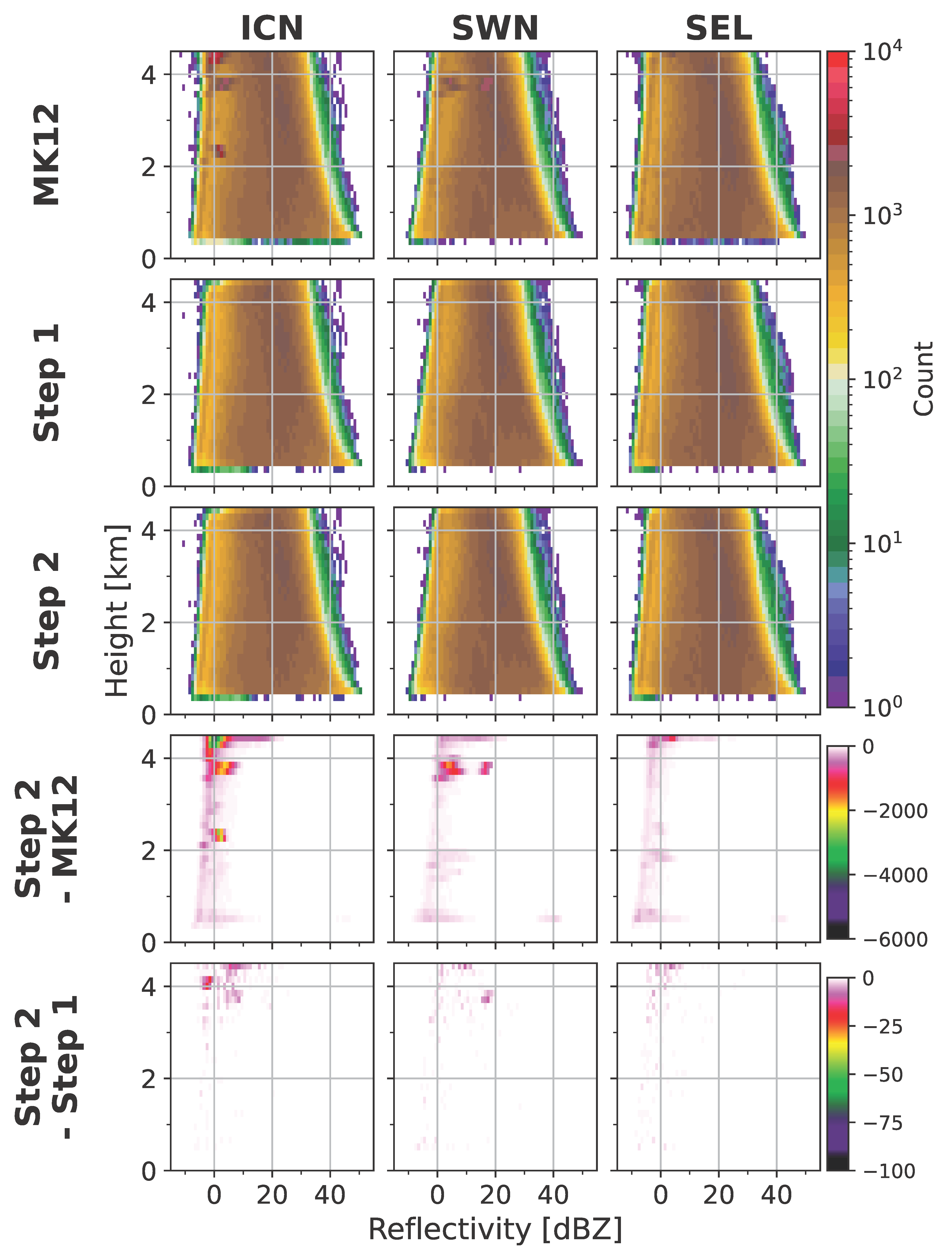
To further validate the algorithm’s performance, we conducted a more systematic and statistical assessment with a larger sample size. In Figure 6, we present the Contoured Frequency by Altitude Diagram (CFAD) of reflectivity for each major step of the algorithm: prior to the application of the algorithm (MK12), after the removal of interference using fuzzy logic (Step 1), and following despeckling (Step 2). The algorithm was applied and evaluated using all available datasets (2021–2023) across three MRR sites, except for the period used to construct the fuzzy logic algorithm (i.e., 23 August–2 September 2021, at ICN and SWN).
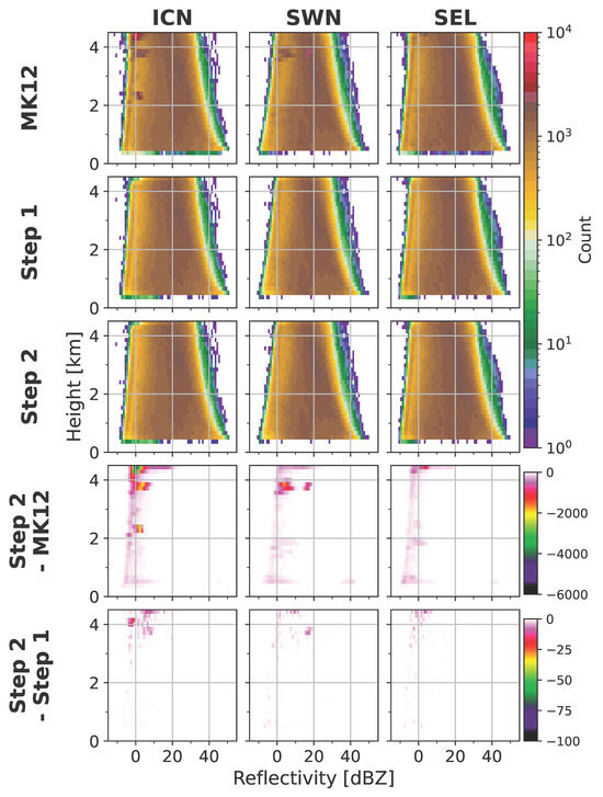
Figure 6.
CFADs of reflectivity for each major step of the algorithm. From top to bottom: CFADs after applying the MK12 algorithm, after performing interference lines’ removal (denoted as “Step 1”), after performing despeckling (denoted as “Step 2”), the difference between “Step 2” and “MK12” CFADs, and the difference between “Step 2” and “Step 1” CFADs. From left to right: ICN, SWN, and SEL sites, with all data except for the period used to construct the fuzzy logic algorithm.
The CFADs for ICN and SWN revealed that more than 1000 spurious counts, resulting from interference lines, were identified at altitudes exceeding 3.5 km and at ~2.3 km. At ICN, these interference lines extended to higher altitudes, affecting the maximum range gates within the −5 to 10 dBZ interval. In contrast, at SWN, the interference lines impacted altitudes up to 4 km, influencing three different reflectivity ranges near 0–10 dBZ and 17 dBZ. These signals were completely eliminated after Step 1, enabling us to interpret the CFAD with meteorological signals only. Despeckling (Step 2) produced minimal changes from the CFAD after Step 1, with differences of fewer than 30 counts. The difference between Step 2 and MK12 indicated that approximately 1000 to 4000 spurious signals were identified and removed. The CFAD for the SEL site showed very few signals associated with interference lines (at 1.8 km, 2.3 km, and 4.2 km), all of which were removed. What we would like to highlight is that the algorithm showed good performance even at the independent SEL site, which was not included during the development of the algorithm.
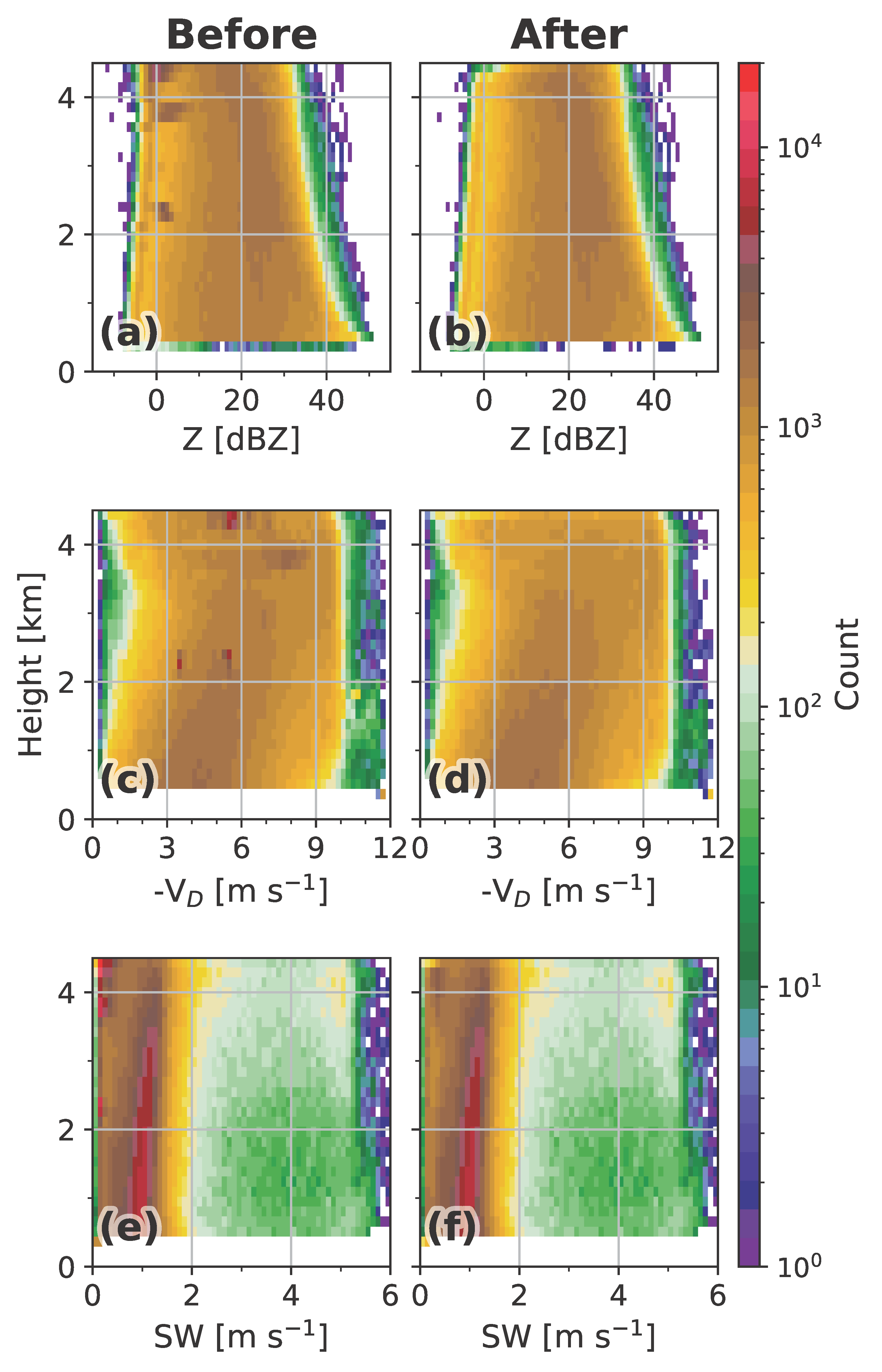
Figure 7 presents the CFAD for the ICN site, including not only reflectivity but also Doppler velocity and spectrum width. As shown in Figure 6, the algorithm successfully eliminated all spurious signals from the reflectivity field. The Doppler velocity exhibited a broad range of spurious signals between 4 and 9 m s−1, making it difficult to detect such signals based solely on Doppler velocity (also supported by the smallest weight of Vr in Table 3). Using the fuzzy logic algorithm, these signals were also effectively removed. In the spectrum width, counts exceeding 10,000 near 0 m s−1, largely attributed to interference lines, were removed, leading to a CFAD that represented a natural distribution of meteorological signals.
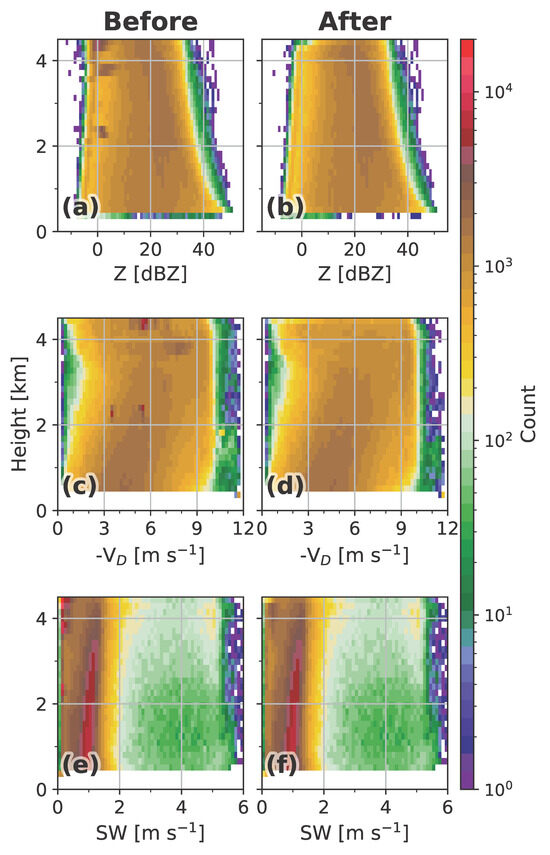
Figure 7.
CFADS of (a,b) reflectivity, (c,d) Doppler velocity, and (e,f) spectrum width for ICN site. Similar to Figure 5, each column represents the data before (denoted as “Before”, corresponding to the data after the MK12 algorithm) and after applying the algorithm (denoted as “After”).
We evaluated the algorithm using all available data from the CFAD analysis. However, this approach has qualitative limitations; therefore, we also quantitatively examined the performance using a smaller number of samples that we labeled subjectively. For this labeling process, we utilized data collected from three sites in 2022 and 2023. We combined data from ICN for 14 days, SWN for 17 days, and SEL for 6 days, resulting in a total of 37 days of data and 42,316 labeled interference line samples. Additionally, we combined data from ICN for 7 days, SWN for 6 days, and SEL for 15 days, yielding a total of 28 days of data and 328,178 labeled precipitation samples.
As a result, we obtained 41,920 true positives (i.e., correctly detected and removed labeled noise), 396 false negatives (i.e., instances where labeled noise was not detected), 8559 false positives (i.e., labeled precipitation misidentified as interference lines), and 319,619 true negatives (i.e., labeled precipitation that was not removed). These numbers corresponded to a probability of detection (POD) of 0.9906, a false alarm ratio (FAR) of 0.1696, and a critical success index (CSI) of 0.8240. This indicates that, when interference lines are present, the algorithm can effectively remove most of them, leaving only 1% remaining. However, approximately 17% of the samples removed by our algorithm contained precipitation, suggesting an aggressive tendency. These cases were likely very weak reflectivities observed in the CFAD (Figure 6) that predominantly followed the sensitivity curve. Except for a few research topics where these signals are critical, this tendency can be considered acceptable for most applications.
4. Discussion and Conclusions
This study successfully developed and validated a fuzzy-logic-based algorithm for detecting and removing interference lines from MRR-2 data. We utilized eight effective fuzzy membership variables to enhance the algorithm’s performance. In addition to traditional fuzzy logic techniques, we designed a membership function that accounts for the multiple modes of reflectivity due to the presence of interference lines at various altitudes and the variability in reflectivity between altitudes. This membership function was utilized to update the predefined membership function and further enhance the performance. Additionally, an optional despeckling procedure was introduced to further enhance the data quality. The CFAD analysis confirmed that the algorithm effectively removed interference lines while preserving meteorological signals, significantly improving data quality and enabling more accurate MRR-2 data interpretation.
To ensure high data quality, we recommend initially assessing the presence of interference lines using CFADs or time–height diagrams. This approach enables us to determine the necessity of applying the algorithm and whether adjustments in configuration settings, such as the minimum height index, are required. Interference lines are often observed in MRR-2 data; they could be nearly absent throughout the observation period (for instance, interference lines were absent in the SEL data from 2021 and 2022). In cases where the time–height diagram does not suggest the presence of interference lines, the need to apply this algorithm is reduced. Given the POD of 0.9906 and FAR of 0.1696, it may be beneficial to consider its potential to eliminate a few weak precipitation echoes. By limiting the algorithm’s application to specific sites and certain dates where spurious data are detected, the potential elimination of some meteorological echoes can be minimized, thereby maximizing data quality. Nonetheless, in situations where the dataset is too large for pre-assessment or where semi-real-time processing is necessary, applying the algorithm to all data is unlikely to significantly impact accurate data interpretation, since instances of mistakenly eliminating meteorological echoes are rare (Figure 6). Thus, applying this algorithm in real time for such cases would not be an inappropriate choice and could be considered a practical option. For reference, the algorithm took ~15 s to process one-day data on a single core of an Intel(R) Xeon(R) Gold 6154 CPU operating at 3.00 GHz.
The algorithm developed in this study is publicly available as open-source. It offers the flexibility to adjust various parameters through a configuration file. Utilizing the compactness and cost effectiveness of MRR-2 systems, which facilitate the easy installation of multiple units, MRR-2 has been widely deployed in field campaigns and operational settings. Given the ongoing use of MRR-2 in understanding the vertical structure of precipitation systems, our algorithm is expected to make a significant contribution to improving data quality for data affected by interference lines. We also believe this algorithm has broad applicability to any MRR2 dataset. Since our algorithm is based on gate index rather than height and the membership variables do not significantly depend on gate resolution, it is unlikely to be substantially influenced by MRR2 configuration or climate regime. We have also confirmed that the algorithm performed well at the independent SEL site.
Author Contributions
Conceptualization, K.K. and G.L.; methodology, K.K. and G.L.; software, K.K.; validation, K.K. and G.L.; formal analysis, K.K. and G.L.; investigation, K.K. and G.L.; resources, K.K. and G.L.; data curation, K.K. and G.L.; writing—original draft preparation, K.K.; writing—review and editing, G.L.; visualization, K.K.; supervision, G.L.; funding acquisition, G.L. All authors have read and agreed to the published version of the manuscript.
Funding
This work was funded by the Korea Meteorological Administration Research and Development Program “Observing Severe Weather in Seoul Metropolitan Area and Developing Its Application Technology for Forecasts” under Grant (KMA2018-00125).
Data Availability Statement
The software is available at https://github.com/Kwonil-Kim/MRR2_interference_line_removal (accessed on 15 October 2024). The data presented in this study are available on request from the corresponding author.
Acknowledgments
The authors would like to thank the participants of the field campaign “Korea Precipitation Observation Program: international collaborative experiments for Mesoscale convective system in Seoul metropolitan area” (KPOP-MS), hosted by the Korea Meteorological Administration (KMA). We appreciate the National Institute of Meteorological Sciences (NIMS) for providing the data used in this study. We also thank the students and researchers at CARE, KNU for constructive discussions and their valuable insights. The authors particularly thank Jihye Jung from KNU for assisting in preparing the validation data.
Conflicts of Interest
The authors declare no conflicts of interest.
References
- Minder, J.R.; Letcher, T.W.; Campbell, L.S.; Veals, P.G.; Steenburgh, W.J. The Evolution of Lake-Effect Convection during Landfall and Orographic Uplift as Observed by Profiling Radars. Mon. Weather Rev. 2015, 143, 4422–4442. [Google Scholar] [CrossRef]
- Adirosi, E.; Baldini, L.; Tokay, A. Rainfall and DSD Parameters Comparison between Micro Rain Radar, Two-Dimensional Video and Parsivel2 Disdrometers, and S-Band Dual-Polarization Radar. J. Atmos. Ocean. Technol. 2020, 37, 621–640. [Google Scholar] [CrossRef]
- Chang, W.-Y.; Lee, G.; Jou, B.J.-D.; Lee, W.-C.; Lin, P.-L.; Yu, C.-K. Uncertainty in Measured Raindrop Size Distributions from Four Types of Collocated Instruments. Remote Sens. 2020, 12, 1167. [Google Scholar] [CrossRef]
- Kim, K.; Bang, W.; Chang, E.; Tapiador, F.J.; Tsai, C.; Jung, E. Impact of Wind Pattern and Complex Topography on Snow Microphysics during International Collaborative Experiment for PyeongChang 2018 Olympic and Paralympic Winter. Atmos. Chem. Phys. 2021, 21, 11955–11978. [Google Scholar] [CrossRef]
- Chang, W.-Y.; Yang, Y.-C.; Hung, C.-Y.; Kim, K.; Lee, G. Estimating the Snow Density Using Collocated Parsivel and MRR Measurements: A Preliminary Study from ICE-POP 2017/2018. EGUsphere 2024. [Google Scholar] [CrossRef]
- Maahn, M.; Kollias, P. Improved Micro Rain Radar Snow Measurements Using Doppler Spectra Post-Processing. Atmos. Meas. Tech. 2012, 5, 2661–2673. [Google Scholar] [CrossRef]
- Garcia-Benadi, A.; Bech, J.; Gonzalez, S.; Udina, M.; Codina, B.; Georgis, J.-F. Precipitation Type Classification of Micro Rain Radar Data Using an Improved Doppler Spectral Processing Methodology. Remote Sens. 2020, 12, 4113. [Google Scholar] [CrossRef]
- Ferrone, A.; Billault-Roux, A.-C.; Berne, A. ERUO: A Spectral Processing Routine for the Micro Rain Radar PRO (MRR-PRO). Atmos. Meas. Tech. 2022, 15, 3569–3592. [Google Scholar] [CrossRef]
- METEK. MRR Physical Basics Version 5.2.0.1; Metek GmbH: Elmshorn, Germany, 2017; p. 20. Available online: https://www.inscc.utah.edu/~hoch/CFOG/4DHIRAJ/mrr-physicalbasics.pdf (accessed on 18 August 2024).
- Thériault, J.M.; Déry, S.J.; Pomeroy, J.W.; Smith, H.M.; Almonte, J.; Bertoncini, A.; Crawford, R.W.; Desroches-Lapointe, A.; Lachapelle, M.; Mariani, Z.; et al. Meteorological Observations Collected during the Storms and Precipitation Across the Continental Divide Experiment (SPADE), April–June 2019. Earth Syst. Sci. Data 2021, 13, 1233–1249. [Google Scholar] [CrossRef]
- Billault-Roux, A.-C.; Grazioli, J.; Delanoë, J.; Jorquera, S.; Pauwels, N.; Viltard, N.; Martini, A.; Mariage, V.; Le Gac, C.; Caudoux, C.; et al. ICE GENESIS: Synergetic Aircraft and Ground-Based Remote Sensing and In Situ Measurements of Snowfall Microphysical Properties. Bull. Amer. Meteor. Soc. 2023, 104, E367–E388. [Google Scholar] [CrossRef]
- Thurai, M.; Bringi, V.; Wolff, D.; Pabla, C.; Lee, G.; Bang, W. Aspects of Rain Drop Size Distribution Characteristics from Measurements in Two Mid-Latitude Coastal Locations. Environ. Sci. Proc. 2023, 27, 14. [Google Scholar] [CrossRef]
- Durán-Alarcón, C.; Boudevillain, B.; Genthon, C.; Grazioli, J.; Souverijns, N.; Van Lipzig, N.P.M.; Gorodetskaya, I.V.; Berne, A. The Vertical Structure of Precipitation at Two Stations in East Antarctica Derived from Micro Rain Radars. Cryosphere 2019, 13, 247–264. [Google Scholar] [CrossRef]
- Kulie, M.S.; Pettersen, C.; Merrelli, A.J.; Wagner, T.J.; Wood, N.B.; Dutter, M.; Beachler, D.; Kluber, T.; Turner, R.; Mateling, M.; et al. Snowfall in the Northern Great Lakes: Lessons Learned from a Multisensor Observatory. Bull. Amer. Meteor. Soc. 2021, 102, E1317–E1339. [Google Scholar] [CrossRef]
- McMurdie, L.A.; Heymsfield, G.M.; Yorks, J.E.; Braun, S.A.; Skofronick-Jackson, G.; Rauber, R.M.; Yuter, S.; Colle, B.; McFarquhar, G.M.; Poellot, M.; et al. Chasing Snowstorms: The Investigation of Microphysics and Precipitation for Atlantic Coast-Threatening Snowstorms (IMPACTS) Campaign. Bull. Amer. Meteor. Soc. 2022, 103, E1243–E1269. [Google Scholar] [CrossRef]

Disclaimer/Publisher’s Note: The statements, opinions and data contained in all publications are solely those of the individual author(s) and contributor(s) and not of MDPI and/or the editor(s). MDPI and/or the editor(s) disclaim responsibility for any injury to people or property resulting from any ideas, methods, instructions or products referred to in the content. |
© 2024 by the authors. Licensee MDPI, Basel, Switzerland. This article is an open access article distributed under the terms and conditions of the Creative Commons Attribution (CC BY) license (https://creativecommons.org/licenses/by/4.0/).