Category-Based Interactive Attention and Perception Fusion Network for Semantic Segmentation of Remote Sensing Images

Abstract

With the development of CNNs and the application of transformers, the segmentation performance of high-resolution remote sensing image semantic segmentation models has been significantly improved. However, the issue of category imbalance in remote sensing images often leads to the model’s segmentation ability being biased towards categories with more samples, resulting in suboptimal performance for categories with fewer samples. To make the network’s learning and representation capabilities more balanced across different classes, in this paper we propose a category-based interactive attention and perception fusion network (CIAPNet), where the network divides the feature space by category to ensure the fairness of learning and representation for each category. Specifically, the category grouping attention (CGA) module utilizes self-attention to reconstruct the features of each category in a grouped manner, and optimize the foreground–background relationship and its feature representation for each category through the interactive foreground–background relationship optimization (IFBRO) module therein. Additionally, we introduce a detail-aware fusion (DAF) module, which uses shallow detail features to complete the semantic information of deep features. Finally, a multi-scale representation (MSR) module is deployed for each class in the CGA and DAF modules to enhance the description capability of different scale information for each category. Our proposed CIAPNet achieves mIoUs of 54.44%, 85.71%, and 87.88% on the LoveDA urban–rural dataset, and the International Society for Photogrammetry and Remote Sensing (ISPRS) Vaihingen and Potsdam urban datasets, respectively. Compared with current popular methods, our network not only achieves excellent performance but also demonstrates outstanding class balance.

1. Introduction

Recently, due to ongoing improvements in remote sensing image technology, achieving high-quality semantic segmentation of these images has emerged as a fundamental and the most talked about task in remote sensing image processing. This technique is essential for applications including urban planning [1], land cover classification [2], and land use planning [3].The main goal of semantic segmentation is to label each pixel of the input image with its category. However, the complex texture information and varying scales of remote sensing image categories make it difficult for traditional methods like random forests (RFs) [4] and support vector machines (SVMs) [5] to perform precise and efficient semantic segmentation, making this a highly challenging task.

With the successful and organic integration of convolutional neural networks (CNNs) into an increasing number of tasks [6], their application in remote sensing semantic segmentation tasks has demonstrated excellent feature extraction and model representation capabilities. Particularly, the advent of the fully convolutional network (FCN) [7] marked the first realization of end-to-end pixel-level segmentation. However, the roughness of the spatial recovery process in the FCN led to insufficiently detailed segmentation outcomes. To resolve this, Ronneberger et al. [8] proposed UNet, which introduced skip connections to compensate for the loss of feature information and employed more upsampling operations to achieve finer segmentation results, thereby further enhancing segmentation accuracy. Nevertheless, UNet did not further refine the integration of low-level features from the encoder with high-level features from the decoder, resulting in the network’s inability to fully differentiate and utilize these features.

CNNs have demonstrated exceptional feature extraction and representation capabilities in image segmentation tasks, but the limited field of view of convolutional kernels also restricts their ability to process contextual information. To tackle this, Chen et al. [9] developed atrous spatial pyramid pooling (ASPP), employing atrous convolutions at various sampling rates to parallelly capture multi-scale image context. Zhao et al. [10] proposed the pyramid pooling module (PPM), which aggregates multi-scale features using regions of different sizes. However, the context information aggregated through pooling and atrous convolutions was relatively coarse, failing to effectively capture global context, and thus did not achieve the desired effect. With the successful application of transformers in the visual field, a new solution to this problem has emerged [11,12]. The visual transformer (ViT) [13] utilizes the self-attention (SA) mechanism to enable a globally weighted representation of each position, thereby enhancing the model’s perception of global context and achieving significant results. However, its high computational cost becomes a major barrier when processing large-scale remote sensing images. Subsequently, the Swin transformer [14] and HMANet [15] have significantly improved the computational efficiency of self-attention on remote sensing images through strategies like windowing and pooling. Chen et al. [16] points out that, although the enhanced ViT architecture has advantages in modeling long-term dependencies, it often overlooks local spatial features. More and more work [17,18,19] is beginning to explore the organic integration of CNNs and transformers, but the focus of these efforts is on enhancing the feature extraction and modeling capabilities of segmentation models through the technical means of CNNs and transformers, without further refinement based on the characteristics of the tasks during the modeling process.

Remote sensing images usually contain rich feature information and usually cover multiple categories. Therefore, compared with general segmentation tasks that are single-target and relatively standardized in content, the remote sensing semantic segmentation model should take the characteristics of the task into more consideration, and the model and modules should be designed to fit the task more closely. Firstly, as shown in Figure 1, remote sensing semantic segmentation often involves multiple categories, and the samples of different categories are imbalanced. These categories not only differ greatly in the overall number of pixel samples, with remote sensing images showing distinct characteristics in different areas [20] (e.g., buildings occupy most of the area in urban regions, while rural regions have fewer buildings), but also show substantial fluctuations in the proportion of each category within local areas of images (e.g., the closer to the city center one goes, the more buildings and fewer trees there are). This imbalance in data and variability in content can lead to similarly imbalanced model performance. Secondly, although the deep features of the network contain rich semantic and category information, their low resolution limits the accuracy of feature representation, leading to blurry edges and details in the segmentation results. While the shallow features are rich in high-resolution detail information, they are relatively primitive and have a gap in expression with the high-level semantics of deep features. To achieve precise segmentation, effectively utilizing the detailed information from the shallow features of the network is particularly important. Therefore, the network’s category balance and the utilization of detailed information are aspects that should receive more attention in remote sensing semantic segmentation tasks. The following sections will explore these two aspects in detail.

On one hand, the general image segmentation networks [7,8] learn all the information as a whole during the segmentation process, and only comb the class information at the output of the model. Empirically, this kind of overall learning for remote sensing images with many and uneven categories easily leads to the learning ability of the model being biased towards the categories with a large proportion of samples, while the categories with fewer samples do not have enough feature space and parameters to be represented and learnt. Therefore, we believe that reducing the squeezing between categories during the learning process of the model and ensuring that each category has enough space to learn and represent is the key to dealing with remote sensing images with imbalanced categories and balancing the performance of the segmentation model. Recent studies [15,21,22] have shown that there is a strong relationship between the channels of the feature map and the categories. Inspired by this, we propose category-based combing decoding. As shown in Figure 2, different from general feature processing, we group the features and deploy the modules according to categories, and each category is decoded in its own feature space, as a way to give the vulnerable categories enough space to learn and represent, and to allow features to be expressed in a clearer way. Additionally, considering that group split limits the utilization of information between groups, we propose the interactive foreground–background relationship optimization (IFBRO), which improves the representation of the foreground and background within each category through interactions between categories.

On the other hand, the feature information of remote sensing images is complex and variable, and the detail information in shallow features is indispensable for achieving accurate pixel-level segmentation. Although the low-level features contain rich detail information such as edges, colors, textures, etc., there are different feeling fields and feature expressions between them and the high-level features. Improper fusion of the two types of features can cause the information from shallow features to become noise within the deep features, interfering with the expression of high-level semantics. Some work [18,23] has demonstrated that while direct summing operations on these two features are quick, they lower segmentation accuracy. To better fuse the two different features, we propose perceptual fusion to align the fields of view of the two features and achieve pixel-level fine fusion.

From the above two points, we introduce the category-based interactive attention and perception fusion network (CIAPNet), a novel semantic segmentation model for remote sensing images based on an encoder–decoder architecture. Unlike the traditional decoding approach, in order to enhance the network model’s ability to adapt to the category imbalance of remote sensing images, we propose the category-based transformer to reconstruct the encoder’s features in the form of categories. We use CGA as the attention module of the transformer to reconstruct the input features using self-attention grouped by categories, and optimize the self-attention weights for each category using IFBRO embedded in CGA to improve the representation relationship between foreground and background. In addition, we propose a detail-aware fusion (DAF) module to achieve fine fusion with deeper feature categories based on the perception of shallow features. Finally, we design a multi-scale representation (MSR) module deployed categorically as the feedforward network for CGA and DAF, using different scales of fields of view to enhance the descriptive capability of features at various scales. Our primary contributions are summarized as follows.

• We propose a new CNN-coded transformer-decoded remote sensing semantic segmentation network CIAPNet based on the characteristics of remote sensing images. Information spaces are divided for each category, and the features of the backbone network are reconstructed by category, achieving balanced learning of the network across all categories. Experiments conducted on three varied remote sensing image datasets reveal that the method performs exceptionally well and the network adapts effectively to the category imbalance in remote sensing images.
• We propose CGA that processes features by grouping them according to category, using multi-head self-attention to enable clearer categorical representation of the encoder’s features. An IFBRO module is embedded to interact with the attention information of different categories, distinguishing the foreground and background of each category and clarifying the representational relationship between them.
• The DAF module is proposed to expand the perceptual field of shallow detailed features using dilated percept. Complete the semantic details of deep features based on the perception of context and categories from detail features. In addition, by introducing MSR deployed by category as the feedforward network, the expression capability of CGA and DAF for each category is further enhanced from a multi-level, multi-scale perspective.

2. Related Work

2.1. Semantic Segmentation for Remote Sensing with CNN Methods

The FCN [7] was the first to use a CNN network for end-to-end semantic segmentation of remote sensing images, setting the stage for future research in remote sensing segmentation methods [24,25]. However, the UNet encoder–decoder structure has a U-shaped network [8] that employs skip connections to progressively restore spatial resolution, mitigating the effects of reduced spatial resolution during the encoding phase. Its excellent performance has made it a mainstream framework for semantic segmentation of remote sensing images, inspiring many new methods [26]. However, the complex content and large-scale variation of remote sensing images are still extremely challenging for convolution with a limited sensory field. In order to solve the problem of CNNs with limited perception, recent studies have incorporated the attention mechanism into the network to extract contextual information. LANet, proposed by Lei et al. [27], enhances local contextual information by using chunking to compute attention, and integrates high-level features and low-level features through the attention mechanism in an embedded manner. The attention bilateral context network A2-FPN [28] employs a feature pyramid network (FPN) to encode semantic features at various scales and boosts multi-scale feature learning via attention-guided feature aggregation. Niu et al. [15] proposed a new hybrid multi-attention network (HMANet) that builds spatial and channel multi-branching and multi-perspective attention, and incorporates the class information into the channel attention to improve each class’s discriminative ability.

2.2. Semantic Segmentation for Remote Sensing with Transformer Methods

The initial attempt at transformer-based semantic segmentation was conducted by the segmentation transformer (SETR) [11], while subsequent models such as Segmenter [29] and SegFormer [30] further demonstrated the effectiveness of transformers in modeling contextual information for semantic segmentation tasks. Particularly, the Swin transformer proposed by Liu et al. [14] performs self-attention within divided windows while creating interactions between adjacent windows by shifting them. This windowed self-attention method greatly reduces the computational resources required for applying it to remote sensing images. However, TransUNet [31] has highlighted that the results produced by purely transformer-based networks are not satisfactory, as transformers focus only on global modeling and lack the capability to extract local features. Consequently, there has been an increasing amount of research exploring effective hybrid mechanisms between CNNs and transformers. For example, CTMFNet [17] effectively integrates CNN and transformer backbones, using attention to merge CNNs’ local information with transformers’ global context. UnetFormer [18] learns global–local context using CNN and transformer with high computational efficiency to achieve real-time segmentation of RS images. DC-Swin [32] uses transformer to extract multi-scale global context feature information and efficiently aggregates multi-scale transformer features through dense links. CMTFNet [23], proposed by Wu et al., enables transformers to extract rich multi-scale global context information and channel information. Zhang et al. [19] proposed LSRFormer with a CNN and transformer interspersed structure, where transformer blocks are added after each CNN stage of a purely convolutional network to complement the global information.

The development of semantic segmentation research in remote sensing has greatly benefited from advancements in the CV field of deep learning, particularly from the work in the field of image classification, which is also a classification task, and has learned many techniques and network structure lessons. Current remote sensing semantic segmentation methods are similar to the techniques and feature processing in the image classification field, with CNN-based methods focusing on enhancing the contextual information modeling capabilities of convolutional networks, and transformer-based methods focusing on higher attention efficiency and more organic integration with CNNs. While these improvements continuously enhance the performance of remote sensing semantic segmentation models, they also prompt us to reflect on the differences between the two tasks. The biggest difference between the two is that, for the same image, image classification targets only one class, while semantic segmentation involves multiple classes. Processing multiple classes of features as a whole may lead to a lack of sensitivity of the network to class and an imbalance in performance. Hong et al. [33] points out that data from different tasks have distinct characteristics, and model design should be more tailored to the data characteristics of the task. Therefore, in the study of semantic segmentation for remote sensing images, which often have complex and highly imbalanced categories, it is crucial to consider the characteristics and relationships between different categories while pursuing the model’s vertical modeling capability for targets. To explore this issue, we propose to divide the overall features in terms of categories to ensure that each category has a relatively fair space for learning and representation, and better grooming and representation of features in the form of decoding of category interactions. Compared with other methods, CIAPNet not only excels in performance but also shows better category balance in remote sensing images during experiments.

3. Methodology

3.1. Overview

Figure 3 illustrates the overall structure of our designed CIAPNet. The network uses an encoder–decoder architecture, HRNet [34], which serves as the encoder backbone to capture multi-scale information from high-resolution input images, minimizing information loss from reduced spatial resolution in remote sensing images. The decoder part is mainly composed of CGA, DAF, and Group MSR. The class-based transformer, consisting of CGA and MSR, allocates and specifies individual feature spaces for each category, reconstructing the features of each category from the overall features in a category-grouped manner, enhances the segmentation model’s adaptability for learning from remote sensing images with imbalanced class samples. Among them, CGA’s purpose is to reconstruct the encoder’s features by category using self-attention deployed according to category, and optimize the relationship between foreground and background by distinguishing foreground and background information of each category through IFBRO. DAF aims to enhance the perceptual capabilities of shallow features, utilizing their abundant detail information to refine deep semantic layers. MSR’s goal is to improve the model’s descriptive ability for features at different scales in remote sensing images through a multi-level, multi-scale perspective.

Specifically, the high-resolution RGB remote sensing image $X\in {\mathbb{R}}^{3\times H\times W}$ is input into our network, where the CNN backbone network, HRNet, first extracts the multi-scale feature information $F_i\in {\mathbb{R}}^{C_i\times H\times W}$, $C_i\in \{32,64,128,256\}$, and $i\in \{1,2,3,4\}$. To facilitate the alignment and fusion of feature maps at different scales, we unify the channel size to $32\times N$ using a $3\times 3$ convolution, where N is the number of categories. Then, the feature, $F_i$, is divided into category features, $F_{ij}\in {\mathbb{R}}^{32\times H\times W}$, each with a channel size of 32. These features are then input into CGA to reconstruct the features of each category using self-attention and are connected with the residual. Subsequently, the features enter the category-deployed MSR to obtain the output of CBT. Then, through the fusion module, the features are concatenated with the corresponding category in $F_{i-1}$, and a $3\times 3$ convolution is used to unify the feature channels of each category from 64 to 32, producing the input ${\mathrm{F\prime }}_{i-1}$ for the next layer’s CGA. This can be mathematically expressed as, $j\in \{1,\dots ,N\}$:

$$\begin{array}{cc}\hfill F{A}_i& =F_i+\mathrm{CGA}\left(F_i\right)\hfill \end{array}$$

(1)

$$\begin{array}{cc}\hfill F{T}_{i,j}& =\mathrm{MSR}\left(F{A}_{i,j}\right)\hfill \end{array}$$

(2)

$$\begin{array}{cc}\hfill F_{i-1,j}^{\prime }& =\mathrm{Conv}\left(\mathrm{Cat}\left(F_{i-1,j},\mathrm{Upsample}\left(F{T}_{i,j}\right)\right)\right)\hfill \end{array}$$

(3)

where $F_i$ and $F{A}_i$ are the features of the i-th layer of the backbone network and the output of CGA, respectively. $F{T}_i$ is the output feature of the class-based transformer, and $F{\mathrm{T\prime }}_{i-1,j}$ and ${\mathrm{F\prime }}_{i-1,j}$ represent the Jth category feature, respectively. The operation $\mathrm{Cat}(·)$ represents the concatenation operation, $\mathrm{Upsample}(·)$ means twice the upsampling, and $\mathrm{Conv}(·)$ represents a convolution function with a kernel size of $3\times 3$.

Subsequently, $F{T}_2$ is fed into the DAF module to be fused with the shallow features, $F_1$, of the backbone network, and the fused representations of each category are optimized through Group MSR. Finally, we concatenate the features of each class into a whole and use a $1\times 1$ convolution to convert the number of channels to the number of categories. The predicted results are upsampled to the same size as the input image using bilinear interpolation, resulting in the final predicted segmentation mask. Additionally, we introduce auxiliary losses to supervise the features of each category output by the CBT, enhancing the interactive learning among categories on the channel level in CGA and achieving better model performance.

3.2. Category-Grouped Attention

Self-attention is an important means of obtaining contextual information, and its application in remote sensing semantic segmentation tasks greatly enhances the global modeling capabilities of models. However, self-attention treats features as a whole, which leads to a lack of sensitivity to the categories within the features. This type of learning can more easily lead to imbalances in model performance, especially in the case of remote sensing images with imbalanced samples. Therefore, we proposed the CGA module from the perspective of channels and categories. By defining the information space for each category on the channel level, we ensure that disadvantaged categories also have sufficient information to represent their features. Additionally, multi-head self-attention is deployed separately for each category to re-represent the input features by category, as shown in Figure 3.

First, we divide the feature information, X, from the CNN network along the channel dimension into groups according to the number of categories, where each part has a channel size of ${\displaystyle \frac{C}{N}}$, serving as CGA inputs $X_j\in {\mathbb{R}}^{{\displaystyle \frac{C}{N}}\times H\times W}$, where C represents the channel dimension, H and W denote the height and width of the feature map, and N indicates the number of segmentation categories. Subsequently, each category’s features are input into their corresponding self-attention to compute their attentional information. In order to save computational overheads, we use window-based multi-head self-attention (W-MHSA) [14]. As illustrated in the CGA in Figure 3, in W-MHSA, $X_j$ is processed through $1\times 1$ convolutions and window partitioning operations to generate the corresponding $Q_j$, $K_j$, $V_j\in {\mathbb{R}}^{h\times w^2\times {\displaystyle \frac{C}{hN}}}$. We set the window size, w, to 8 and the number of heads, h, to 4. For ease of representation and description here, we omit the number of windows. Then, the attention weights corresponding to $A_j$ are calculated by matrix multiplication of $Q_j$ and $K_j$. The process described above can be expressed as follows, $j\in \{1,\dots ,N\}$:

$$\begin{array}{c}\hfill A_j=\left({\displaystyle \frac{Q_j{K}_j^T}{\sqrt{d}}}\right)+b\end{array}$$

(4)

where d represents the channel dimension, and b is the relative position bias.

While dividing feature information into categories for their respective modeling helps to protect the learning of weaker categories and balance the performance of the model, the segregation of information between categories may miss valuable cross-channel interactions, resulting in less rich representations learned by each category, and therefore unlike simply applying self-attention to each category separately. In the CGA module, we designed the IFBRO module to interactively compare the attention information of different categories, thereby determining the foreground and background pixels of each category. By improving the relationship between the foreground and background, the attention affinity matrix is optimized, enabling clearer feature representation of the foreground and background for each category. The following describes the interactive optimization process of the attention affinity matrix in detail.

To optimize the foreground–background relationship of the attention information, A, for each category, we first need to find and determine the foreground–background pixel positions for each category. As shown in Figure 4, we perform an average pooling operation with a kernel size of $w^2\times h$ on the attention information matrix, A (where h represents the perception of multiple heads and $w^2$ represents the perception of other pixels) to obtain the perception matrix, P, for each pixel in each category. Subsequently, we determine the foreground information of the current pixel based on the maximum value of the pixel in the category and mark this category with 1, while other categories are considered background information and marked with −1, thus obtaining the foreground–background pixel position matrix, C, for each category. The specific process is expressed as follows:

$$\begin{array}{cc}\hfill P& =\mathrm{AvgPooling}\left(A\right)\hfill \end{array}$$

(5)

$$\begin{array}{cc}\hfill C& =\mathrm{Max}\text{\_}\mathrm{Value}\text{\_}\mathrm{Mark}\left(P\right)\hfill \end{array}$$

(6)

where A is the attention score matrix for each category, with a size of $N\times w^2\times w^2\times h$, $\mathrm{AvgPooling}(·)$ represents the average pooling operation applied to the last two dimensions of A using a pooling kernel of size $w^2\times h$, and $\mathrm{Max}\text{\_}\mathrm{Value}\text{\_}\mathrm{Mark}(·)$ represents a judgment function that assigns a maximum mark of 1 and −1 for the others.

For the learning and representation of each category, we always hope that the relationship between the foreground and background is sensitive and distinct; this means that the foreground is positively correlated with the foreground and negatively correlated with the background, and vice versa for the background. Next, we optimize the attention scores of each category in A based on the foreground–background relationship criterion. According to the foreground–background relationship criterion and the foreground–background pixel position matrix, C, we generate the foreground–background relationship mask, $C^{\prime }$, for each category. Each row in $C^{\prime }$ represents the foreground–background relationship of that pixel in the current category, and this relationship is used to optimize the attention affinity matrix, A. The relationship mask, $C^{\prime }$, is multiplied by the attention weights normalized by the softmax function to obtain the optimized attention weights, $A^{\prime }$. $A^{\prime }$ clarifies the relationship between the foreground and background, increases the distance between the foreground and background, and enhances the attention’s ability to represent the foreground and background. Finally, the optimized weights, $A^{\prime }$, are multiplied by the V matrix to obtain the final output of CGA. The specific expression is as follows:

$$\begin{array}{cc}\hfill C^{\prime }& =C^T\times C\hfill \end{array}$$

(7)

$$\begin{array}{cc}\hfill A^{\prime }& =C^{\prime }·\mathrm{Softmax}\left(A\right)\hfill \end{array}$$

(8)

$$\begin{array}{cc}\hfill X_{\mathrm{out}}& =A^{\prime }\times V\hfill \end{array}$$

(9)

3.3. Detail-Aware Fusion

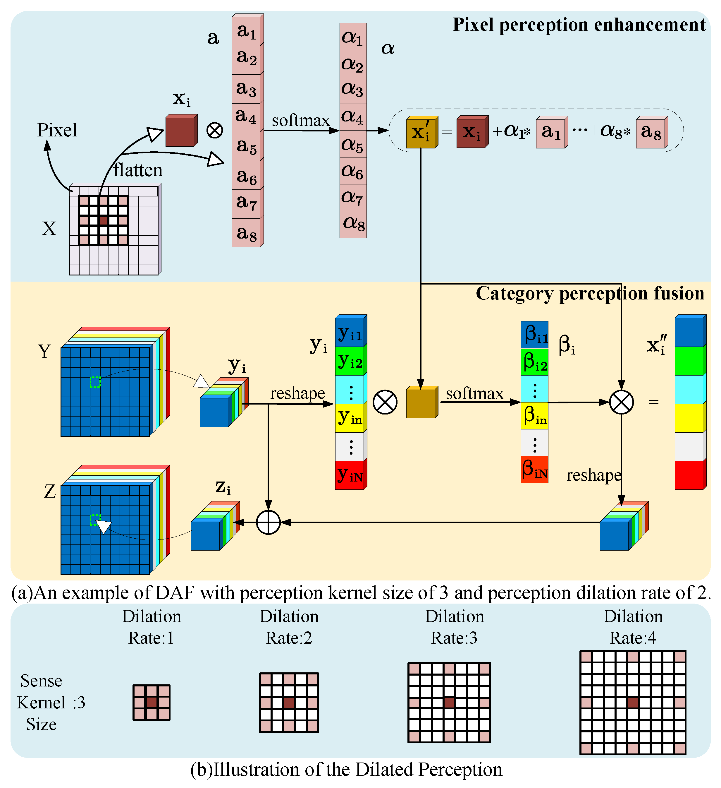
Rich spatial detail information in shallow features, such as color, texture, and edges, is an important basis for the precise segmentation of details in various categories in remote sensing images. Effectively utilizing shallow features and achieving precise fusion with deep semantics is a critical step in ensuring model performance. Unlike common fusion methods such as addition, concatenation, weighting, and attention, the key point of our proposed DAF is to enhance the perception of shallow features to align with the field of view of deep features and to fuse deep features based on the category perception of shallow feature pixels. The following explains our method in detail.

3.3.1. Pixel Perception Enhancement

Shallow features have rich detail information, but the smaller perceptual field of shallow features tends to cause them to miss important contextual information. As shown in Figure 5b, inspired by dilated convolution [35], we adopt the style of the dilated convolution kernel so that each pixel perceives the other pixels in a dilated form. Without losing information through pooling, we increase each pixel’s perception of its surroundings in the shallow features, adding contextual awareness to the shallow features.

3.3.2. Category Perception Fusion

The semantic information of shallow features and deep features is inconsistent, and direct additive fusion may destroy or drown the deep semantics. Inspired by the channel attention mechanism, we generate the affinity matrix for the fusion of the two based on the shallow feature’s perception of the categories of the deep feature’s channel dimensions, and assign each pixel of the shallow feature to each category of the deep feature, so as to realize the fine-tuning of the deep semantics.

Our goal is to utilize shallow detail features to finely adjust the semantic information of each category in the deep features. Therefore, we need to use a $1\times 1$ convolution to align the channel sizes of the shallow feature, $F_1$, with the channel sizes of each category in upsampled deep feature Y to obtain the detail information input of the module $X\in {\mathbb{R}}^{{\displaystyle \frac{C}{N}}\times H\times W}$, where C is the channel size of deep feature Y, N is the number of segmentation target categories, and H and W are the feature map sizes. To more effectively merge shallow feature X with deep feature Y, we first perform pixel perception enhancement on X. This enhances the perceptual ability of shallow features, aligns the field of view of both features, and narrows the expression gap with deep feature Y. We adopt the dilated form for pixel enhancement, as shown in Figure 5b. Specifically, as illustrated in Figure 5a, a matrix multiplication operation is performed on the n perceived pixels, a, within the dilated perception region of pixel $X_i$ to compute the correlation with the surrounding pixels. Subsequently, the perception scores for these pixels are obtained by the Softmax function. Based on the scores, we generate the pixel perceptually enhanced pixel $x_i^{\prime }$. The above process can be expressed as $i\in \{1,2,3,\dots ,H\times W\}$, $j\in \{1,2,3,\dots ,n\}$:

$$\begin{array}{cc}\hfill \alpha & =\mathrm{Softmax}(x_i\times a)\hfill \end{array}$$

(10)

$$\begin{array}{cc}\hfill x_i^{\prime }& =x_i+\sum _{j=1}^n{\alpha }_j\times a_j\hfill \end{array}$$

(11)

Next, precise adjustments to the semantic information in the deep features are achieved through the category-aware fusion operation. Specifically, we multiply $x_i^{\prime }$ with the features of each category on the pixel $y_i$ channel, and obtain the perception scores, $\beta$, for $x_i^{\prime }$ with respect to each category of $y_i$ using the Softmax function. Based on the perception of both, we generate the detail-perceived pixels, $x_i^{\prime \prime }$, for each category, and add them to $y_i$ to obtain the fused feature pixel $z_i$. The specific expression is as follows:

$$\begin{array}{cc}\hfill \beta & =\mathrm{Softmax}(y_i\times x_i^{\prime })\hfill \end{array}$$

(12)

$$\begin{array}{cc}\hfill x_i^{\prime \prime }& =\beta \times x_i^{\prime }\hfill \end{array}$$

(13)

$$\begin{array}{cc}\hfill z_i& =y_i+x_i^{\prime \prime }\hfill \end{array}$$

(14)

3.4. Multi-Scale Representation

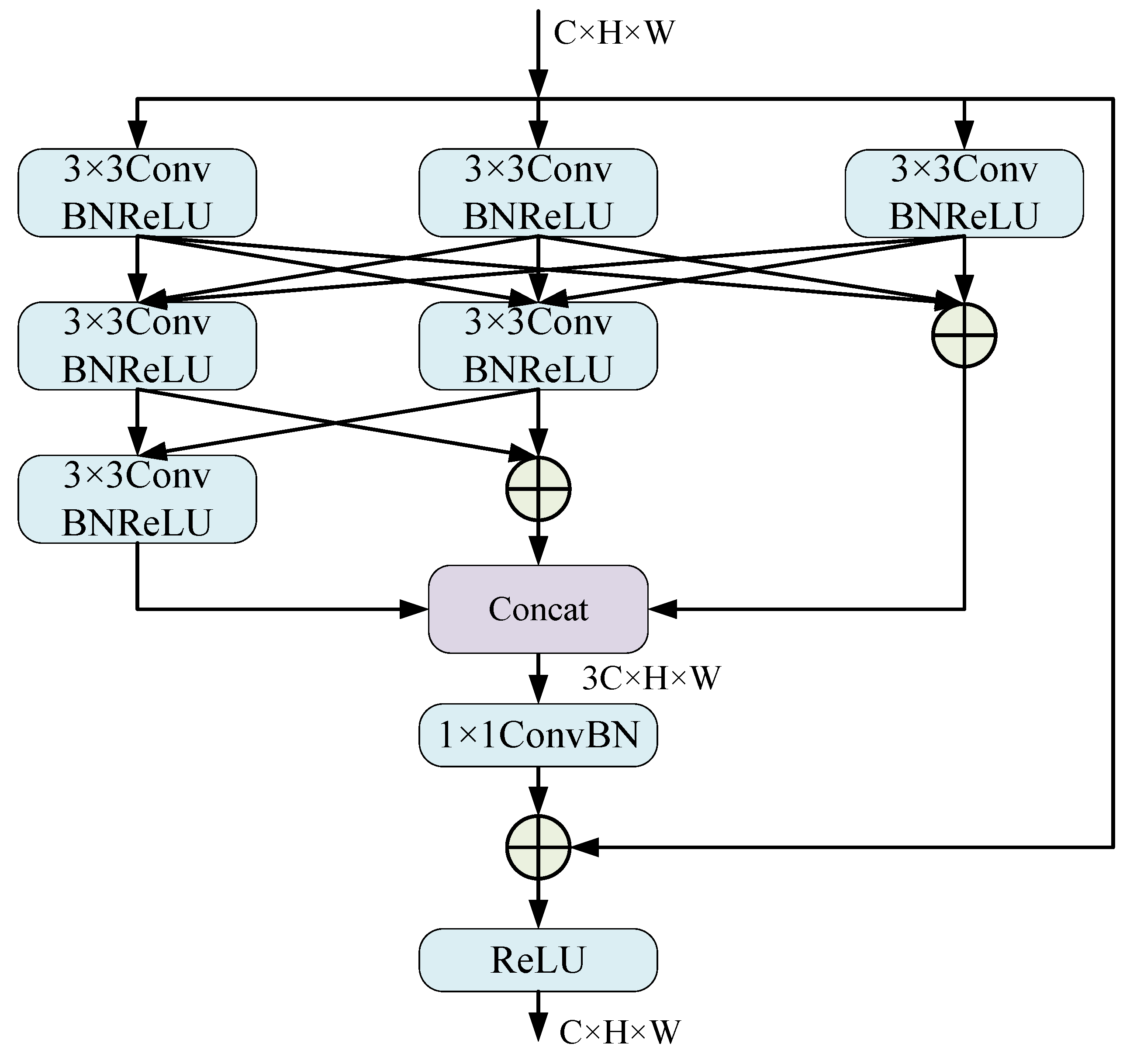
Objects in remotely sensed images typically have large-scale variations, and each feature also typically has multiple aspects at different scales. Therefore, when describing objects in remote sensing images, it is necessary to summarize and express them from different scale perspectives and various characteristics. In order to enhance the decoder’s ability to describe each category, we designed a MSR module, which uses a multi-layer $3\times 3$ convolution to form multi-level fields of view of different sizes, and deploy as shown in Figure 2 as the feedforward network for CGA and DAF, grouped by category.

As shown in Figure 6, we divide the receptive field into three levels. To ensure that smaller receptive fields can also describe different features, we use three branches in the first-level receptive field, each deploying a $3\times 3$ convolution module. Each convolution is followed by a BatchNorm and ReLU function, and the outputs of the three branches are combined to describe features with a $3\times 3$ receptive field. Similar to the first level, we deploy two $3\times 3$ convolution modules in the second-level receptive field to extract different information, using the output of the first level as input. The two branches are added together to obtain the output of the $5\times 5$ receptive field. The third-level $7\times 7$ receptive field uses a single $3\times 3$ convolution module to continue learning from the output of the previous level. Finally, we use a concatenation operation to integrate the descriptions from the three different receptive fields. A $1\times 1$ convolution is used to adjust the channel size, followed by a BatchNorm function, and a residual connection is added with the input. After activation with a ReLU function, we obtain multi-scale features described by the three different sizes of receptive fields.

3.5. Loss Function

As shown in Figure 3, in order to achieve better results for this decoding of combing interactions by categories, we not only supervise the optimization of the final segmentation prediction map but also add additional auxiliary headers to supervise the features of each category of the CBT outputs individually according to the ground truth. Therefore, we use the main loss, $L_M$, and auxiliary loss, $L_A$, to train our overall network structure. We use a combination of Dice loss, $L_D$, and cross-entropy loss, $L_{CE}$, as the primary loss, defined as follows:

$$\begin{array}{cc}\hfill L_M& =L_{CE}+L_D\hfill \end{array}$$

(15)

In addition, for the output sum of the three-layer CBT module, we use N sets of auxiliary heads of $3\times 3$ convolutional layers with BatchNorm and ReLU, $1\times 1$ convolutional layers, segmentation predictions with aggregated channel size 1 for features of N categories, respectively, and output by upsampling, while supervised by using the cross-entropy loss function, $L_{CE}$, as an auxiliary loss ($L_A$) function. In order to better unite the primary and auxiliary losses, we set the scaling factor of the auxiliary loss, $\alpha$. Thus, our total loss function, $L_{\mathrm{total}}$, is defined as follows:

$$\begin{array}{cc}\hfill L_A& =L_{CE}\hfill \end{array}$$

(16)

$$\begin{array}{cc}\hfill L_{\mathrm{total}}& =L_M+\alpha L_A\hfill \end{array}$$

(17)

4. Experiments and Analysis

4.1. Datasets

4.1.1. ISPRS Vaihingen

This dataset comprises 33 orthophotos, each with an average resolution of $2494\times 2064$ pixels and a 9 cm ground sampling distance (GSD). Every image contains three bands, near-infrared, red, and green, in addition to the digital surface model (DSM) and normalized DSM (NDSM). The dataset spans six categories: impervious surfaces, buildings, low vegetation, trees, cars, and clutter/background. We use 16 images for training and the remaining 17 for testing.

4.1.2. ISPRS Potsdam

This dataset consists of 38 orthophotos, each measuring $6000\times 6000$ pixels with a ground sampling distance (GSD) of 5 cm. Each image includes near-infrared, red, green, and blue bands, as well as corresponding DSM and NDSM. It covers the same six categories as the Vaihingen dataset. We use 24 images for training and the remaining 14 for testing.

4.1.3. LoveDA Dataset

This dataset comprises 5987 high-resolution optical remote sensing images (GSD 0.3 m), each sized $1024\times 1024$ pixels, and includes 7 land cover categories: building, road, water, barren, forest, agriculture, and background. We use 2522 images for training, 1669 for validation, and the remaining 1796 for testing.

4.2. Evaluation Metrics

To evaluate the effectiveness of our proposed model, we use mean F1 score (mF1), mean intersection over union (mIoU), and overall accuracy (OA), based on the cumulative confusion matrix as evaluation metrics. The calculations for OA, mF1, and mIoU are as follows:

$$\begin{array}{c}\hfill \mathrm{OA}={\displaystyle \frac{TP+TN}{TP+FP+TN+FN}}\end{array}$$

(18)

$$\begin{array}{c}\hfill \mathrm{mF}1={\displaystyle \frac{1}{n}}\sum _{i=1}^n{\displaystyle \frac{2·T{P}_i}{2·T{P}_i+F{P}_i+F{N}_i}}\end{array}$$

(19)

$$\begin{array}{c}\hfill \mathrm{mIoU}={\displaystyle \frac{1}{n}}\sum _{i=1}^n{\displaystyle \frac{T{P}_i}{T{P}_i+F{P}_i+F{N}_i}}\end{array}$$

(20)

where n is the number of target segmentation categories, $T{P}_n$ is true positive, $T{N}_n$ is true negative, $F{P}_n$ is false positive, and $F{N}_n$ is the number of false negative pixels.

4.3. Experimental Setting

All experiments were conducted on a single NVIDIA GeForce RTX 3090 GPU using the PyTorch framework for consistency. We used HRNet [34], pretrained on ImageNet, as the backbone. The AdamW optimizer was employed, with a batch size of 8, an initial learning rate of $6\times {10}^{-4}$, and a weight decay of 0.01. The learning rate followed a cosine annealing schedule. Images were randomly cropped into $512\times 512$ patches and augmented with random scaling and rotation during training. The number of epochs was set to 30 for LoveDA, 225 for Vaihingen, and 105 for Potsdam. During testing, test-time augmentation (TTA) strategies such as vertical and horizontal flipping were applied.

4.4. Ablation Studies of Network Components

4.4.1. Ablation Analysis of Loss Function

To enable the network to better adapt to and learn this category-based interactive decoding, the model employs auxiliary loss to supervise the learning of each category separately. Therefore, we first conducted experiments to analyze the relationship between the primary loss and the auxiliary loss, denoted by the ratio $\alpha$. Specifically, we set the ratio $\alpha$ from 0 to 1 in intervals of 0.2 and conducted experiments on the Vaihingen dataset. The experimental results are shown in

Table 1. Comparison of different weighting parameters, $\alpha$, for auxiliary losses on the Vaihingen dataset.

$\mathit{\alpha }$	0.0	0.2	0.4	0.6	0.8	1.0
mIoU (%)	85.08	85.27	85.71	85.62	85.60	85.30
mF1 (%)	91.76	91.89	92.14	92.09	92.07	91.90

*Bold* indicates the best value.

. It can be observed that the model performs best when $\alpha$ is 0.4. Notably, using the auxiliary loss to supervise the features output by the class-based transformer module is highly effective for learning each category, leading to improvements of 0.63% and 0.38% in the mIoU and mF1 metrics, respectively.

4.4.2. Effect of Each Component of CIAPNet

To assess the effectiveness of each CIAPNet component, we performed ablation experiments on the ISPRS Vaihingen and Potsdam datasets. Our baseline model is a U-shaped network using HRNet as the backbone, and we superimpose the proposed method sequentially, and observe and analyze the effectiveness of each component as well as the changes in model complexity. The results of the experiment are shown in

Table 2. Results of ablation experiments for the proposed method on the Vaihingen dataset.

Dataset	Method	Params (Mb)	FLOPs (Gbps)	mF1 (%)	mIoU (%)
	Base	30.69	202.25	90.16 (↑ 0.00)	82.49 (↑ 0.00)
	CGA	30.57	197.42	91.00 (↑ 0.84)	83.84 (↑ 1.35)
	CGA + MSR	31.63	205.06	91.40 (↑ 1.24)	84.49 (↑ 2.00)
Vaihingen	DAF	30.50	196.57	90.90 (↑ 0.74)	83.65 (↑ 1.16)
	DAF + MSR	30.85	219.87	91.12 (↑ 0.96)	84.03 (↑ 1.54)
	CGA + DAF + MSR	31.97	227.97	91.76 (↑ 1.60)	85.08 (↑ 2.59)
	CGA + DAF + MSR + AuxLoss	31.97	227.97	92.14 (↑ 1.98)	85.71 (↑ 3.22)
	Base	30.69	202.25	92.07 (↑ 0.00)	85.53 (↑ 0.00)
	CGA	30.57	197.42	92.78 (↑ 0.71)	86.76 (↑ 1.23)
	CGA + MSR	31.63	205.06	92.95 (↑ 0.88)	87.05 (↑ 1.52)
Potsdam	DAF	30.50	196.57	92.33 (↑ 0.26)	86.00 (↑ 0.47)
	DAF + MSR	30.85	219.87	92.54 (↑ 0.47)	86.34 (↑ 0.81)
	CGA + DAF + MSR	31.97	227.97	93.16 (↑ 1.09)	87.44 (↑ 1.91)
	CGA + DAF + MSR + AuxLoss	31.97	227.97	93.43 (↑ 1.36)	87.88 (↑ 2.35)

, where MSR stands for Group MSR deployed in groups by class, and AuxLoss refers to the auxiliary loss of supervising the features of each class separately.

Our proposed method shows significant improvements on the Vaihingen dataset. Using three CGA modules as decoders for the U-shaped network, the model’s mIoU score increases by 1.35% and the mF1 score by 0.84% compared with the baseline. Deploying MSR as a feedforward network of CGA modules to form a complete category-based transformer further improves model performance by 0.65% in mIoU and 0.4% in mF1. Similarly, we incorporate DAF into the baseline decoder to help fuse the high- and low-level features, and this fusion method enhances mIoU by 1.16% and mF1 by 0.74%. Using Group MSR as a feedforward network for DAF, the model’s mIoU is further improved by 0.38% and mF1 by 0.22%. Adding DAF, CGA, and MSR to the network improves the model’s mIoU by 2.59% and mF1 by 1.6%. When we use supervised auxiliary loss by category for the features, the final network performance reaches 85.71% for mIoU and 92.14% for mF1.

Our proposed method also enhances model performance on the Potsdam dataset. We deployed CGA in a network that gives the model a 1.23% and 0.71% improvement in mIoU and mF1, respectively. Adding the MSR-based feedforward network to CGA continues to improve the model’s performance by 0.29% in mIoU and 0.17% in mF1. Similarly, when only DAF is deployed in the decoder, it improves the model’s mIoU and mF1 by 0.47% and 0.26%, respectively, and when Group MSR, a feedforward network, is added to DAF, the model’s mIoU and mF1 are further improved by 0.34% and 0.21%, respectively. Incorporating all modules into the network increases the mIoU by 1.91% and mF1 by 1.09% over the baseline. After using the auxiliary loss supervision class-based transformer, the mIoU of the network reaches 87.88% and the mF1 reaches 93.43%.

Since the modules in our proposed category-based interactive decoder are deployed similarly to grouped convolutions, where each group only processes the features of the current group, the overall complexity of the decoder is relatively lightweight. As observed from the changes in parameters and FLOPs in the table, when CGA or DAF is added to the decoder, the model’s parameters and FLOPs remain almost identical to the baseline. The final parameters and FLOPs of the model compared with the baseline are increased by 1.26 Mb and 25.72 Gbps, with the decoder’s parameters accounting for only 3.94% of the total parameters and 11.28% of the total FLOPs.

4.5. Comparison with State of the Art

We conducted a comparison between our proposed method and the latest advanced methods. In particular, when selecting networks, we aimed to use methods with comparable backbone performance. The specific networks include the following four: [10,21,23,27,36,37,38] based on ResNet-50 [32,39] based on Swin-S [14,22,40] based on HRNet [19,34] based on ConvNeXt-S [41]. At the same time, we also calculated the proportion of each category in the three datasets and included it in the header of the comparison experiment table to facilitate analyzing the advantages of our network over other methods in categories with fewer samples.

4.5.1. Results on Vaihingen Dataset

We conducted a comparison of our method with existing methods using the Vaihingen dataset. The detailed experimental results are provided in

Table 3. Experimental results on the ISPRS Vaihingen dataset.

Method	Imp.surf. (27.81%)	Building (26.01%)	Lowveg. (21.25%)	Tree (22.90%)	Car (1.25%)	OA (%)	mF1 (%)	mIoU (%)
PSPNet [10]	95.67 ± 0.27	93.22 ± 0.18	83.12 ± 0.40	88.78 ± 0.33	77.41 ± 1.45	91.66 ± 0.20	87.64 ± 0.45	78.62 ± 0.65
DeeplabV3+ [36]	96.59 ± 0.09	95.27 ± 0.09	84.15 ± 0.55	89.76 ± 0.23	85.19 ± 0.47	92.96 ± 0.14	90.19 ± 0.24	82.53 ± 0.38
DANet [37]	95.47 ± 0.30	94.18 ± 0.32	82.45 ± 0.71	88.09 ± 0.64	71.17 ± 3.16	91.55 ± 0.45	86.27 ± 1.03	76.90 ± 1.37
LANet [27]	96.60 ± 0.09	94.84 ± 0.07	84.10 ± 0.22	89.68 ± 0.11	87.68 ± 0.53	92.86 ± 0.11	90.57 ± 0.20	83.11 ± 0.32
MANet [38]	96.67 ± 0.02	95.27 ± 0.08	84.18 ± 0.05	89.83 ± 0.18	87.74 ± 0.19	93.00 ± 0.07	90.74 ± 0.09	83.38 ± 0.14
LoG-CAN [21]	96.81 ± 0.02	95.65 ± 0.05	84.61 ± 0.07	89.99 ± 0.02	87.40 ± 0.12	93.25 ± 0.01	90.89 ± 0.04	83.65 ± 0.06
CMFTNet [23]	96.82 ± 0.05	95.48 ± 0.06	84.79 ± 0.27	90.19 ± 0.04	87.51 ± 0.07	93.28 ± 0.01	90.97 ± 0.03	83.76 ± 0.06
DC-Swin [32]	96.96 ± 0.03	96.09 ± 0.10	84.85 ± 0.15	90.24 ± 0.08	86.83 ± 0.53	93.51 ± 0.07	90.99 ± 0.06	83.84 ± 0.09
SACANet [22]	96.88 ± 0.02	95.98 ± 0.03	84.83 ± 0.11	90.12 ± 0.06	88.12 ± 0.33	93.41 ± 0.03	91.18 ± 0.06	84.13 ± 0.11
DOCNet [40]	96.87 ± 0.16	96.06 ± 0.07	85.05 ± 0.11	90.02 ± 0.20	88.82 ± 0.33	93.47 ± 0.06	91.38 ± 0.10	84.44 ± 0.16
ConvLSR-Net [19]	97.08 ± 0.03	96.14 ± 0.10	85.01 ± 0.13	90.38 ± 0.03	88.01 ± 0.16	93.61 ± 0.05	91.32 ± 0.06	84.37 ± 0.11
CIAPNet	97.11 ± 0.01	96.20 ± 0.09	85.55 ± 0.13	90.32 ± 0.09	91.51 ± 0.19	93.75 ± 0.02	92.14 ± 0.03	85.71 ± 0.04

*Bold* indicates the best value.

. From the results, it is evident that our CIAPNet (HRNet) exhibits significant advantages compared with other methods. It not only ranks first in mF1, mIoU, and OA, but also scores the highest in categories such as impervious surfaces, building, low vegetation and car. Particularly in the car category, our method scores 91.51% in the F1 metric, outperforming the second-place SACANet by 2.70%. This proves that CIAPNet’s approach to dividing the feature space by category and the category-interactive decoding are feasible for shaping model performance and effective in improving learning in categories with fewer samples.

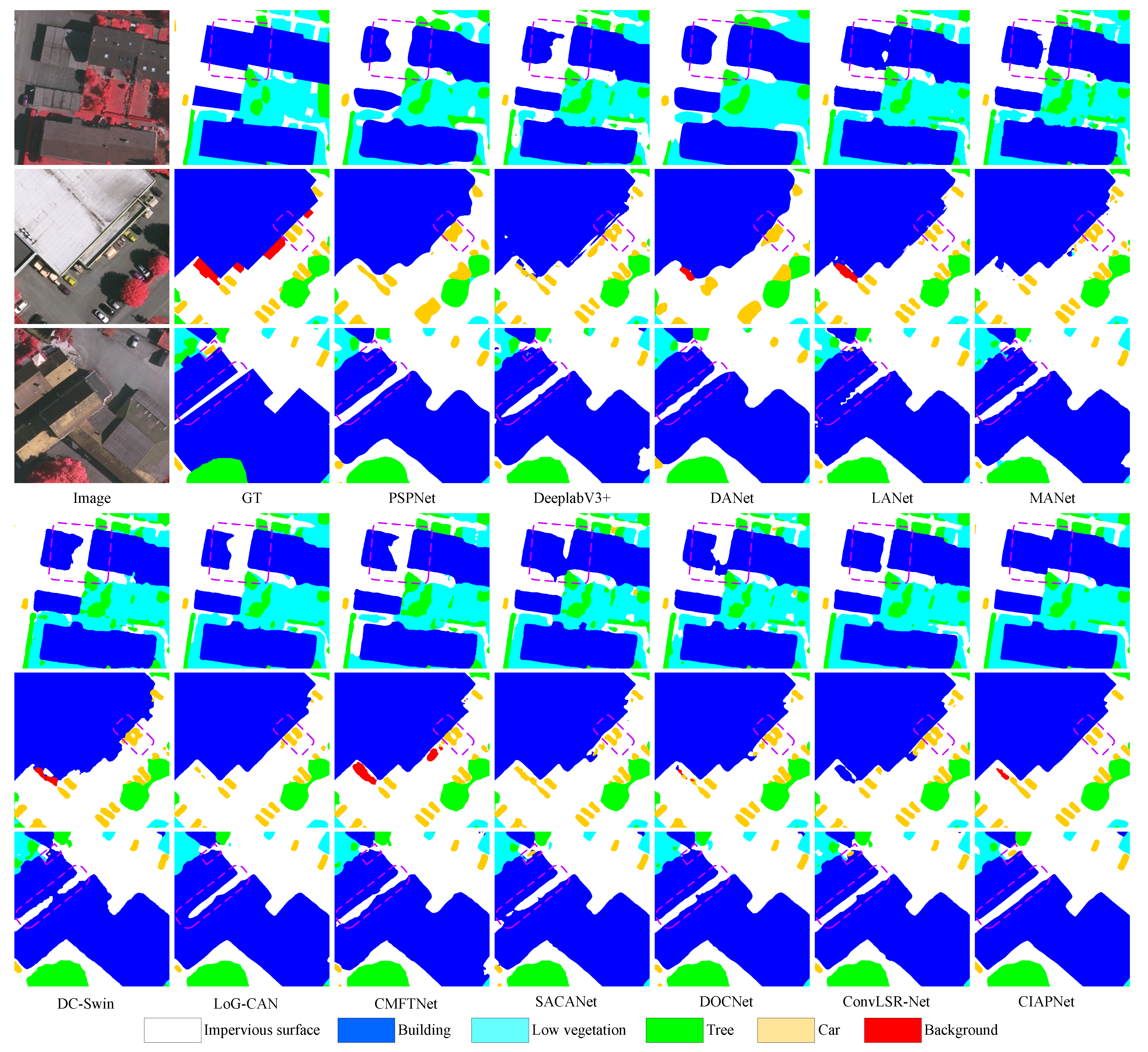
To clearly observe the advantages of our method over others, we compared the visual results of various methods in Figure 7. It can be seen that CIAPNet demonstrates superior segmentation capability compared with other methods. The interaction and perception of various categories enable the model to perform well in complex environments. In the first image, the shadowed portions of the building are very similar to impervious surfaces, leading to misclassification by other methods. However, CGA in our network, through category interaction and comparison, better distinguishes these regions. In the second figure, CIAPNet’s ability to learn well for the less-sampled category allows it to segment each car more accurately compared with other networks. For the blurry and dim boundary information in the third image, all other methods exhibit some degree of boundary blurring, while CIAPNet, through category comparison and surrounding perception, achieves better information extraction and discrimination in blurry areas, resulting in more accurate boundaries.

4.5.2. Results on Potsdam Dataset

To further explore the capabilities of the model, we conducted additional comparisons with current methods on a larger Potsdam dataset, and the experimental results are presented in

Table 4. Experimental results on the ISPRS Potsdam dataset.

Method	Imp.surf. (29.48%)	Building (25.48%)	Lowveg. (22.68%)	Tree (15.73%)	Car (1.75%)	OA (%)	mF1 (%)	mIoU (%)
PSPNet [10]	91.18 ± 0.58	92.86 ± 0.89	83.92 ± 0.44	83.62 ± 1.19	92.12 ± 1.12	87.52 ± 0.77	88.74 ± 0.85	80.01 ± 1.37
DeeplabV3+ [36]	93.85 ± 0.29	96.20 ± 0.16	87.20 ± 0.04	88.79 ± 0.21	95.83 ± 0.25	91.16 ± 0.11	92.37 ± 0.13	86.04 ± 0.22
DANet [37]	91.43 ± 0.09	94.78 ± 0.07	84.91 ± 0.31	87.05 ± 0.20	82.21 ± 0.21	89.03 ± 0.16	88.09 ± 0.17	79.01 ± 0.27
LANet [27]	93.31 ± 0.23	95.67 ± 0.22	86.80 ± 0.20	88.74 ± 0.09	95.99 ± 0.17	90.70 ± 0.14	92.10 ± 0.09	85.58 ± 0.15
MANet [38]	93.44 ± 0.13	95.95 ± 0.27	87.32 ± 0.25	88.90 ± 0.16	96.33 ± 0.06	91.05 ± 0.19	92.39 ± 0.17	86.08 ± 0.28
LoG-CAN [21]	93.98 ± 0.15	96.34 ± 0.20	87.62 ± 0.17	88.81 ± 0.20	96.44 ± 0.41	91.36 ± 0.09	92.60 ± 0.04	86.43 ± 0.08
CMFTNet [23]	94.31 ± 0.07	96.61 ± 0.10	87.89 ± 0.17	89.11 ± 0.17	96.61 ± 0.15	91.70 ± 0.10	92.91 ± 0.10	86.98 ± 0.18
DC-Swin [32]	94.33 ± 0.13	96.94 ± 0.06	87.97 ± 0.03	89.38 ± 0.06	86.31 ± 0.15	91.78 ± 0.07	92.99 ± 0.08	87.11 ± 0.13
SACANet [22]	94.20 ± 0.10	96.62 ± 0.31	87.55 ± 0.22	89.20 ± 0.21	95.98 ± 0.45	91.58 ± 0.11	92.71 ± 0.07	86.63 ± 0.12
DOCNet [40]	94.02 ± 0.10	96.59 ± 0.32	87.55 ± 0.31	89.04 ± 0.13	95.97 ± 0.06	91.34 ± 0.13	92.63 ± 0.09	86.50 ± 0.17
ConvLSR-Net [19]	94.63 ± 0.09	97.10 ± 0.09	88.04 ± 0.10	89.44 ± 0.18	96.35 ± 0.03	91.92 ± 0.09	93.11 ± 0.08	87.33 ± 0.13
CIAPNet	94.54 ± 0.01	97.28 ± 0.20	88.55 ± 0.01	89.76 ± 0.07	96.98 ± 0.09	92.14 ± 0.03	93.43 ± 0.04	87.88 ± 0.07

*Bold* indicates the best value.

. CIAPNet still shows excellent performance and again achieves optimal performance on OA, mF1, and mIoU. On the Potsdam dataset, our MeanF1 and mIoU metrics reach 93.43% and 87.88%, respectively, which is an improvement of 0.55% in mIoU over the next best method, ConvLSR-Net. Notably, in the highly urbanised Potsdam dataset, our network excels in the low vegetation, tree, and car categories with relatively small sample sizes, with the network’s segmentation performance for these categories outperforming that of the next best method by 0.51%, 0.32% and 0.37%. This further illustrates the effectiveness of our proposed method for the less-sample category, which is valuable for improving and shaping the performance of models based on deep learning methods.

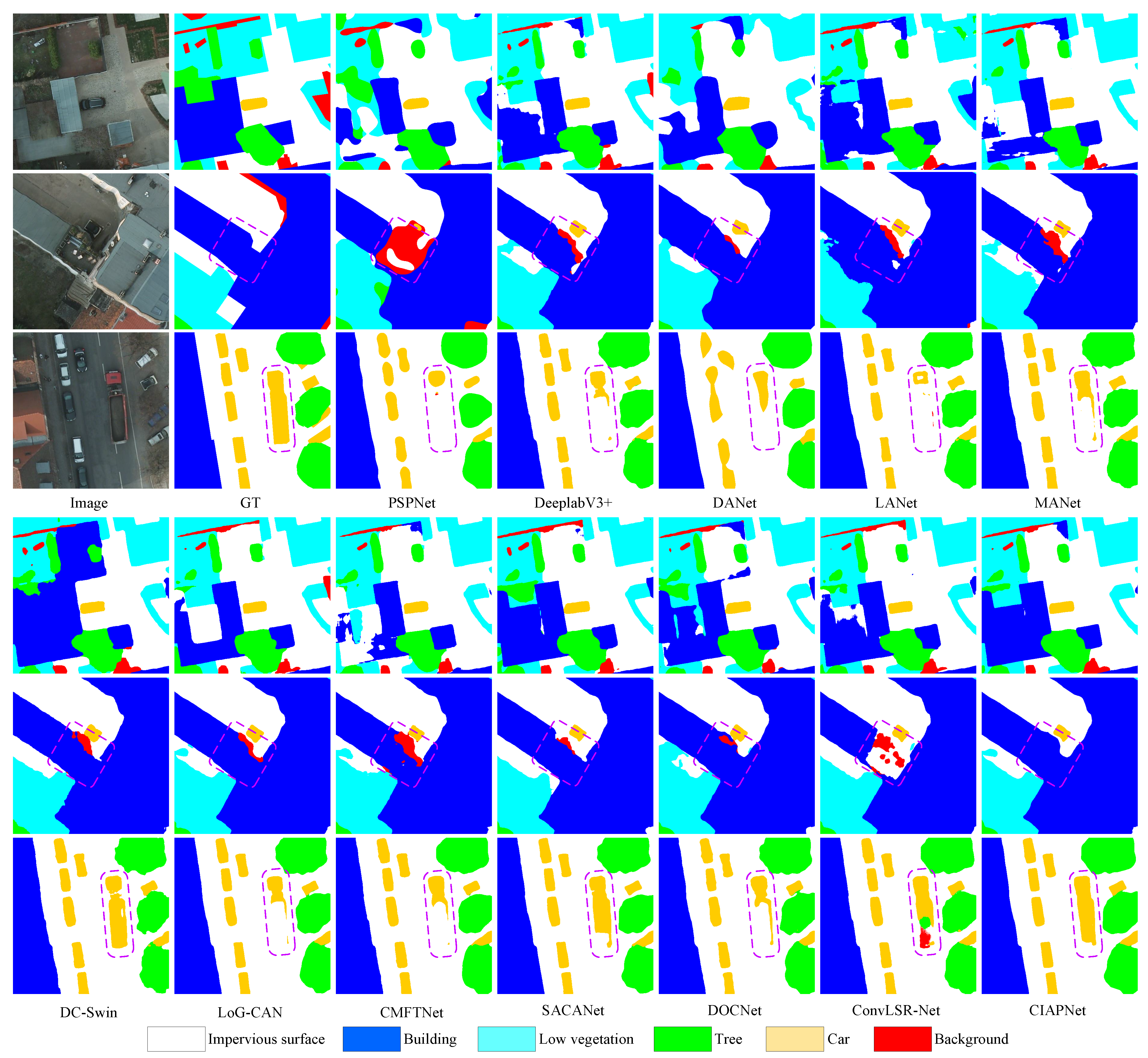
To visually demonstrate the advantages of our proposed method, we also compared the experimental results on the Potsdam dataset, as shown in Figure 8. In the first image, the rooftops of buildings and the ground are remarkably similar, and all other methods are unable to distinguish its category well, while CIAPNet accurately discerns and segments this similar region by comparing the features of the categories through CGA. For the building roofs with cluttered items that are very similar to the background in the second figure, all other networks judge the clutter as the background, while CIAPNet accurately determines the category attribution of these cluttered areas by perceiving the clutter and its surrounding buildings. CIAPNet’s excellent learning ability for the less-sampled category makes it more accurate than other methods in segmenting out the boundary of the car category in the third figure.

4.5.3. Results on LoveDA Dataset

To verify the model’s ability to handle more categories, we conducted further testing and comparisons on the more complex LoveDA dataset. The experimental results are shown in

Table 5. Experimental results on the LoveDA dataset.

Method	Background	Building	Road	Water	Barren	Forest	Agriculture	mIoU (%)
	(35.91%)	(9.51%)	(5.03%)	(8.53%)	(4.87%)	(12.58%)	(23.56%)
PSPNet [10]	50.36 ± 0.20	54.84 ± 0.81	46.59 ± 0.08	50.76 ± 5.58	21.30 ± 1.58	35.65 ± 0.43	44.78 ± 1.65	42.14 ± 2.78
DeeplabV3+ [36]	53.41 ± 0.71	58.61 ± 4.52	54.61 ± 0.26	69.28 ± 0.62	28.55 ± 1.17	43.11 ± 0.72	52.07 ± 5.59	51.27 ± 0.94
DANet [37]	53.16 ± 0.24	58.76 ± 0.61	50.87 ± 0.30	66.90 ± 1.05	28.70 ± 0.45	40.61 ± 0.49	53.54 ± 2.15	49.83 ± 0.12
LANet [27]	52.41 ± 0.37	62.29 ± 0.90	53.64 ± 1.52	65.41 ± 0.62	26.00 ± 4.05	40.30 ± 1.78	48.83 ± 1.17	49.99 ± 0.54
MANet [38]	53.52 ± 0.51	62.40 ± 0.32	53.07 ± 0.36	70.24 ± 0.95	30.72 ± 1.09	42.34 ± 1.42	52.03 ± 0.65	52.05 ± 0.16
LoG-CAN [21]	54.17 ± 0.29	62.88 ± 1.32	53.92 ± 0.40	70.96 ± 0.20	29.46 ± 1.89	41.78 ± 0.61	54.20 ± 1.52	52.21 ± 0.26
CMFTNet [23]	54.31 ± 0.46	62.82 ± 0.38	54.66 ± 1.99	69.77 ± 0.44	28.92 ± 1.84	41.72 ± 1.18	52.90 ± 2.97	52.03 ± 0.26
DC-Swin [32]	53.47 ± 1.42	61.43 ± 1.14	55.47 ± 1.12	70.27 ± 0.09	32.45 ± 2.37	44.06 ± 1.35	58.29 ± 0.87	52.86 ± 0.87
SACANet [22]	52.93 ± 0.47	61.73 ± 2.66	55.08 ± 0.08	68.56 ± 2.54	30.20 ± 2.35	41.47 ± 1.19	50.81 ± 0.84	51.66 ± 0.34
DOCNet [40]	53.51 ± 0.23	61.67 ± 1.41	55.37 ± 0.70	70.65 ± 0.86	32.08 ± 2.08	41.95 ± 0.47	58.74 ± 3.27	52.54 ± 0.31
ConvLSR-Net [19]	51.01 ± 0.34	55.29 ± 3.53	52.14 ± 0.63	66.00 ± 1.01	26.89 ± 0.54	42.83 ± 0.71	48.38 ± 0.88	49.05 ± 0.37
CIAPNet	52.14 ± 1.26	64.80 ± 0.40	55.53 ± 0.61	71.39 ± 0.48	38.95 ± 0.16	43.44 ± 0.73	56.12 ± 1.93	54.47 ± 0.23

*Bold* indicates the best value.

, where the middle section of Table 5 presents the IoU metrics for each category. CIAPNet has the highest score on mIoU, with a 1.61% improvement over the suboptimal method. As shown in the table, our network performs well in the categories with fewer samples, such as building, road, water, and barren, particularly excelling in the barren category, with a 6.5% improvement over the next best method. Additionally, the building and water classes also show a remarkable performance, with mIoU improvements of 1.92% and 0.43%, respectively, over the next best method. This again proves CIAPNet’s excellent ability to handle the disadvantaged category with fewer samples. However, due to the use of window-based self-attention, the attention range is limited to the window size, resulting in insufficient interaction between windows. This limits the ability to model large-scale features, resulting in less outstanding performance in categories with significant feature variations, such as background and forest. Using global self-attention might yield better results, but it would also result in significantly higher computational costs.

The visualization results of the LoveDA validation set are shown in Figure 9. Due to the complex and variable nature of barren terrain, which typically has gradient texture features, other methods cannot accurately segment the first image. However, CIAPNet enhances the learning and differentiation of the disadvantaged barren category, thus performing better than other methods. The use of DAF improves the model’s perception capability, making it superior in distinguishing the relatively blurry features in the second and third images compared with other methods.

4.6. Network Performance Balancing Analysis

4.6.1. Comparison of Performance Balance with State-of-the-Art-Methods

The performance of our proposed model on the above three datasets is outstanding, especially the segmentation results for the lesser sample categories in each dataset are clearer and more accurate. In order to compare the balance of the model for each category, we use the standard deviation to measure the performance of the model for each category. The specific results are shown in

Table 6. Our method compared with the latest advanced methods in terms of standard deviation across categories.

Method	Vaihingen	Potsdam	LoveDA
PSPNet [10]	7.45	4.58	11.50
DeeplabV3+ [36]	5.23	4.14	12.84
DANet [37]	9.91	5.04	12.43
LANet [27]	5.13	4.15	13.41
MANet [38]	5.21	4.10	11.90
LoG-CAN [21]	5.25	4.18	12.55
CMFTNet [23]	5.13	4.15	13.44
DC-Swin [32]	5.41	4.08	12.27
SACANet [22]	5.15	4.10	12.68
DOCNet [40]	5.01	4.11	12.81
ConvLSR-Net [19]	5.20	4.12	12.04
CIAPNet	4.69	4.06	11.30

*Bold* indicates the best value.

, which shows that our model exhibits good equilibrium for all categories in all three datasets, and the standard deviation is the lowest among the methods. This proves that our proposed interactive category-based decoding is very effective in improving the model’s ability to handle fewer sample categories and enhancing the model’s equilibrium.

4.6.2. Impact of Network Components on Performance Balance

To further investigate the impact of our proposed method on the performance of low-sample categories and the overall model performance, we analyzed the performance of various components of the network using the Vaihingen dataset. We sequentially added the modules we proposed to the network, observed their performance across different categories, and used the standard deviation (SD) function to measure the overall balance of the model’s performance. As shown in

Table 7. Network components on the performance balance, where SD is the standard deviation of performance for each category.

Method	Imp.surf.	Building	Lowveg.	Tree	Car	mIoU (%)	SD
		27.81%	26.01%	21.25%	22.90%	1.25%
Base	96.71	95.14	83.43	89.70	85.84	82.50	5.74
CGA	96.86	95.54	83.86	89.73	89.02	83.84	5.27
CGA + MSR	96.88	95.94	84.44	89.99	89.76	84.49	5.09
CGA + DAF + MSR	97.04	96.02	84.99	89.99	90.79	85.08	4.89
CGA + DAF + MSR + AuxLoss	97.11	96.20	85.55	90.32	91.51	85.71	4.69

, the addition of CGA significantly improves the learning ability for low-sample categories, increasing the mIoU of the car category, which only accounts for 1.25% of the samples, by 3.18%. With the coordinated integration of various components, the mIoU of the low-sample car category is improved by 5.67%, and the balance of the network across categories (SD) decreases from 5.74 to 4.69. The experiments demonstrate that our network has excellent learning ability for low-sample categories, while also achieving more balanced overall performance. This is not only due to the decoder’s category-based feature processing, which protects low-sample categories, but also due to IFBRO, which enhances category distinction through cooperative foreground–background reconstruction, leading to balanced overall performance.

4.7. Experiment on CGA

4.7.1. Effectiveness of Group Block Strategy

In order to explore the effectiveness of the strategy of handling features and deploying modules by category in CGA modules, we validated it on several modules that have been fully validated for effectiveness, namely SE [42], CBAM [43], W-MHSA [14], ASPP [9], Ghost [44], and RFB [45]. For fairness, these modules were trained under the same training and testing settings. The related results are shown in

Table 8. The experimental results of applying the class grouping strategy to some popular modules on the Potsdam dataset. The metrics are presented as mIoU, with all values expressed as percentages.

Block	General	Group Block	Group Block + AuxLoss
SE [42]	86.03	86.22	86.23
CBAM [43]	86.50	86.74	86.85
W-MHSA [14]	86.06	86.32	86.55
ASPP [9]	86.36	86.40	86.44
Ghost [44]	85.67	85.80	86.15
RFB [45]	85.84	86.12	86.17

. ’General’ represents the typical method of using modules, ’Group block’ represents the grouping of features and modules by category, and ’AuxLoss’ refers to using auxiliary loss to supervise the learning of features of each category separately after deploying them according to Group block. The metric in the table is mIoU. It can be seen that, after adopting Group block, the performance of these methods improves, with W-MHSA and RFB showing significant gains of 0.26% and 0.28%, respectively. When used in conjunction with auxiliary loss, the improvement of these modules is even more pronounced, especially W-MHSA and Ghost, which show improvements of 0.49% and 0.48% in mIoU compared with general direct use. The results show that Group block improves the learning of modules for each category better than direct use of the modules, and even more so when combined with auxiliary loss.

4.7.2. Optimization Effect of IFBRO on Foreground–Background Relationship in CGA

To verify the effectiveness of category information interaction via IFBRO in CGA, we designed experiments for comparison. We used W-MHSA with the Group block strategy as a baseline, compared it using IFBRO to optimize attention weights, and further compared the performance of IFBRO by supervising each category with auxiliary loss. The specific experimental results shown in

Table 9. Results of the IFBRO pre-background relation optimization experiment in CGA on the Potsdam dataset.

Method	mF1 (%)	mIoU (%)
Base	92.52	86.32
Base + IFBRO	92.78	86.76
Base + IFBRO + AuxLoss	92.87	86.93

*Bold* indicates the best value.

indicate that, through the optimization of foreground–background feature representation by IFBRO, there is a 0.26% and 0.44% improvement in mF1 and mIoU, respectively, and after further supervision using auxiliary losses, the mF1 and mIoU improvements reach 0.35% and 0.61% compared with the baseline. The results demonstrate that optimizing the foreground–background relationship of attention weights through interactive category attention is highly effective in enhancing W-MHSA’s modeling capabilities.

We visualized and compared the output feature maps of the three methods in Table 9 with the general multi-head self-attention output, to visualize the enhancement of the Group block strategy on the expressive ability of each category, and the improvement effect of IFBRO on the pre-background representation of each category. The specific results are shown in Figure 10. From the figure, it can be seen that Group W-MHSA’s feature representation of each category is clearer than the general overall representation, and the feature differences between each category are well represented. After further optimizing the foreground–background feature representation of each category using IFBRO, the relationship between the foreground and background of each category becomes clearer, with the foreground of the current category being more prominent and the background milder. Finally, when we introduce the auxiliary loss to further supervise the features of each category, we can observe that the difference between the foreground and background of each category is more obvious and the foreground–background representation is more accurate.

4.8. Experiment on DAF

4.8.1. The Impact of Class Perception and Pixel Perception

We carried out experiments on the Vaihingen dataset to further analyze the roles of class perception and pixel perception in DAF. We used the direct addition of high- and low-level features as a baseline and incrementally integrated the class perception and pixel perception components of DAF into the experiments. The specific experimental results shown in

Table 10. Experimental results of class perception and pixel perception experiments in DAF on Vaihingen dataset.

Method	mF1 (%)	mIoU (%)
Feature addition	91.81	85.15
Class perception	91.95	85.38
Class perception + pixel perception	92.14	85.71

*Bold* indicates the best value.

indicate that the fusion of the two types of features through class perception, compared with direct addition, improves mIoU by 0.23% and mF1 by 0.14%. After enhancing the pixel perception of shallow features before class perception, the model’s mIoU and mF1 performance further increases, with increases of 0.56% and 0.33%, respectively, compared with just direct addition. The experiment validates the effectiveness of DAF’s perceptual fusion approach.

4.8.2. Pixel Perception Sensitivity to Dilation Rates

To determine the optimal size of the perception kernel and dilation rates for pixel perception enhancement, we conducted experiments on the Vaihingen dataset. In DAF, we used three different sizes of perception kernels and set four different dilation rates, where a dilation rate of 1 means the perception kernel has no dilation. The specific experimental results are shown in

Table 11. Experimental results on perceptual kernel size and perceptual dilation rate in DAF on Vaihingen dataset, where the metrics in the table are mIoU and all values are expressed as percentages.

Dilation Rates	Kernel = 3	Kernel = 5	Kernel = 7
1	85.32	85.57	85.51
2	85.36	85.71	85.56
3	85.57	85.57	85.62
4	85.68	85.36	85.56

*Bold* indicates the best value.

, indicating that the best performance of DAF is achieved with a perception kernel size of 5 and a dilation rate of 2.

4.9. Experiment on MSR

To explore the advantages of the multilevel convolutional field of view consisting of $3\times 3$ convolutions in MSR, we compared the three-layer field of view of 3, 5, and 7 sizes formed in MSR with the general multi-scale field of view consisting of convolutional kernels of 3, 5, and 7 sizes. We conducted experiments on the Potsdam dataset, and the results are shown in

Table 12. Experimental results of MSR versus general multi-scale field of view comparisons on the Potsdam dataset.

Method	Params (Mb)	FLOPs (Gbps)	mIou (%)
3_5_7Conv	0.53	11.57	87.31
MSR	0.35	7.74	87.88

*Bold* indicates the best value.

. It can be seen that MSR has better multi-scale representation compared with general multi-scale representation, with a 0.57% improvement in mIoU, and MSR has a smaller number of parameters and lower FLOPs.

4.10. Model Complexities

Computational efficiency is crucial for the implementation of the framework and is an important metric to evaluate the performance and efficiency of the model. In

Table 13. Results of efficiency analyses.

Method	Backbone	Params (Mb)	FLOPs (Gbps)	mIou (%)
PSPNet [10]	ResNet-50	52.52	807.47	78.62
DeeplabV3+ [36]	ResNet-50	39.75	693.68	82.53
DANet [37]	ResNet-50	47.40	110.85	76.90
LANet [27]	ResNet-50	23.79	132.97	83.11
MANet [38]	ResNet-50	35.86	310.98	83.38
LoG-CAN [23]	ResNet-50	30.91	199.08	83.65
CMFTNet [32]	ResNet-50	30.07	131.07	83.76
DC-Swin [21]	Swin-S	66.90	277.20	83.84
SACANet [22]	HRNet	30.21	226.94	84.13
DOCNet [40]	HRNet	39.12	791.84	84.44
ConvLSR-Net [19]	ConvNeXt-S	68.04	283.59	84.37
CIAPNet (ours)	HRNet	31.97	227.97	85.71

, we count the number of parameters and mIoU performance of each method and obtain the computational amount of the model with the input of a three-channel image of $1024\times 1024$ size. In CIAPNet, the decoding of features in the decoding part is in the form of grouping features by class, and the module of each class only processes the features of the current class, which has a smaller computational amount in comparison with the overall processing of features. As can be seen from Table 13, CIAPNet achieves superior performance compared with other methods, while maintaining a low number of parameters and low computational complexity.

5. Discussion

The unbalanced share of categories in remote sensing images often leads to a bias in the model’s performance towards categories with a large share of samples. In this regard, we propose the CIAPNet model to perform category-based reconstruction of encoder features through category-based interactive decoding. While having competitive performance, it effectively improves the model’s performance on remote sensing images with few sample categories and the balance of the overall model performance. The analysis and validation of our approach through a large number of experiments show that this category-based decoding strategy effectively protects the learning and representation of the less-sample categories, effectively enhances the category sensitivity and feature representation ability of the model through the interaction of pre-background information between the categories, and achieves a more balanced model performance. It is worth noting that the balanced model performance and robustness demonstrated by CIAPNet’s category-based processing strategy for features and modules, as well as the feature interaction between different categories, can provide new ideas for feature processing and module structure for category-based tasks such as medical image segmentation and change detection, and help these tasks to design a network structure that is more in line with the characteristics of the task data.

6. Conclusions

In this paper, we propose a category-based semantic segmentation framework for remote sensing images, CIAPNet, which revisits traditional feature processing patterns. Unlike general holistic feature processing, we partition the feature space based on categories during the decoding phase and reconstruct the features for each category, balancing the model’s ability to learn and represent across categories, while ensuring features are more clearly represented by category. To ensure that categories with fewer samples receive sufficient resources for learning, we propose the CGA module, which processes features and deploys self-attention according to the Group block strategy, along with the category interaction module IFBRO to improve the foreground–background representation relationships across categories. Additionally, we introduce the DAF module to achieve semantic refinement at the pixel level of deep features using shallow features. Finally, we utilize the multi-perspective MSR module to enhance the network’s ability to describe multi-scale features. Experimental results on three datasets verify the effectiveness of our proposed CIAPNet, which also demonstrates outstanding balance. However, as the number of categories increases, this category-based feature processing approach also leads to an increase in the number of feature spaces, as well as the model parameters and computational load. In the future, we will further explore efficient category-based feature processing methods to ensure that the network achieves efficient remote sensing image segmentation while maintaining sensitivity and balance to categories.

References

1. Liu, J.; Cheng, S.; Du, A. ER-Swin: Feature Enhancement and Refinement Network Based on Swin Transformer for Semantic Segmentation of Remote Sensing Images. IEEE Geosci. Remote Sens. Lett. 2024, 21, 5003305. [Google Scholar] [CrossRef]
2. Cheng, S.; Chan, R.; Du, A. CACFTNet: A Hybrid Cov-Attention and Cross-Layer Fusion Transformer Network for Hyperspectral Image Classification. IEEE Trans. Geosci. Remote Sens. 2024, 62, 1–17. [Google Scholar] [CrossRef]
3. Yu, J.; Zeng, P.; Yu, Y.; Yu, H.; Huang, L.; Zhou, D. A Combined Convolutional Neural Network for Urban Land-Use Classification with GIS Data. Remote Sens. 2022, 14, 1128. [Google Scholar] [CrossRef]
4. Pal, M. Random forest classifier for remote sensing classification. Int. J. Remote Sens. 2005, 26, 217–222. [Google Scholar] [CrossRef]
5. Guo, Y.; Jia, X.; Paull, D. Effective Sequential Classifier Training for SVM-Based Multitemporal Remote Sensing Image Classification. IEEE Trans. Image Process. 2018, 27, 3036–3048. [Google Scholar] [CrossRef]
6. Yi, Y.; Zhang, Z.; Zhang, W.; Zhang, C.; Li, W.; Zhao, T. Semantic Segmentation of Urban Buildings from VHR Remote Sensing Imagery Using a Deep Convolutional Neural Network. Remote Sens. 2019, 11, 1774. [Google Scholar] [CrossRef]
7. Long, J.; Shelhamer, E.; Darrell, T. Fully convolutional networks for semantic segmentation. In Proceedings of the IEEE Conference on Computer Vision and Pattern Recognition (CVPR), Boston, MA, USA, 7–12 June 2015; pp. 3431–3440. [Google Scholar]
8. Ronneberger, O.; Fischer, P.; Brox, T. U-Net: Convolutional Networks for Biomedical Image Segmentation. In Proceedings of theMedical Image Computing and Computer-Assisted Intervention—MICCAI 2015, Munich, Germany, 5–9 October 2015; Springer: Berlin, Germany, 2015; pp. 234–241. [Google Scholar]
9. Chen, L.C.; Papandreou, G.; Schroff, F.; Adam, H. Rethinking atrous convolution for semantic image segmentation. arXiv 2017, arXiv:1706.05587. [Google Scholar]
10. Zhao, H.; Shi, J.; Qi, X.; Wang, X.; Jia, J. Pyramid Scene Parsing Network. In Proceedings of the IEEE Conference on Computer Vision and Pattern Recognition (CVPR), Honolulu, HI, USA, 21–26 July 2017; pp. 6230–6239. [Google Scholar]
11. Zheng, S.; Lu, J.; Zhao, H.; Zhu, X.; Luo, Z.; Wang, Y.; Fu, Y.; Feng, J.; Xiang, T.; Torr, P.H.; et al. Rethinking semantic segmentation from a sequence-to-sequence perspective with transformers. In Proceedings of the IEEE/CVF Conference on Computer Vision and Pattern Recognition (CVPR), Nashville, TN, USA, 20–25 June 2021; pp. 6877–6886. [Google Scholar]
12. Zhao, X.; Guo, J.; Zhang, Y.; Wu, Y. Memory-Augmented Transformer for Remote Sensing Image Semantic Segmentation. Remote Sens. 2021, 13, 4518. [Google Scholar] [CrossRef]
13. Dosovitskiy, A.; Beyer, L.; Kolesnikov, A.; Weissenborn, D.; Zhai, X.; Unterthiner, T.; Dehghani, M.; Minderer, M.; Heigold, G.; Gelly, S.; et al. An image is worth 16x16 words: Transformers for image recognition at scale. arXiv 2020, arXiv:2010.11929. [Google Scholar]
14. Liu, Z.; Lin, Y.; Cao, Y.; Hu, H.; Wei, Y.; Zhang, Z.; Lin, S.; Guo, B. Swin Transformer: Hierarchical Vision Transformer using Shifted Windows. In Proceedings of the IEEE/CVF International Conference on Computer Vision (ICCV), Montreal, QC, Canada, 10–17 October 2021; pp. 9992–10002. [Google Scholar]
15. Niu, R.; Sun, X.; Tian, Y.; Diao, W.; Chen, K.; Fu, K. Hybrid Multiple Attention Network for Semantic Segmentation in Aerial Images. IEEE Trans. Geosci. Remote Sens. 2022, 60, 5603018. [Google Scholar] [CrossRef]
16. Li, C.; Zhang, B.; Hong, D.; Zhou, J.; Vivone, G.; Li, S.; Chanussot, J. CasFormer: Cascaded transformers for fusion-aware computational hyperspectral imaging. Inf. Fusion 2024, 108, 102408. [Google Scholar] [CrossRef]
17. Song, P.; Li, J.; An, Z.; Fan, H.; Fan, L. CTMFNet: CNN and Transformer Multiscale Fusion Network of Remote Sensing Urban Scene Imagery. IEEE Trans. Geosci. Remote Sens. 2023, 61, 5900314. [Google Scholar] [CrossRef]
18. Wang, L.; Li, R.; Zhang, C.; Fang, S.; Duan, C.; Meng, X.; Atkinson, P.M. UNetFormer: A UNet-like transformer for efficient semantic segmentation of remote sensing urban scene imagery. ISPRS J. Photogramm. Remote Sens. 2022, 190, 196–214. [Google Scholar] [CrossRef]
19. Zhang, R.; Zhang, Q.; Zhang, G. LSRFormer: Efficient Transformer Supply Convolutional Neural Networks With Global Information for Aerial Image Segmentation. IEEE Trans. Geosci. Remote Sens. 2024, 62, 5610713. [Google Scholar] [CrossRef]
20. Hong, D.; Zhang, B.; Li, H.; Li, Y.; Yao, J.; Li, C.; Werner, M.; Chanussot, J.; Zipf, A.; Zhu, X.X. Cross-city matters: A multimodal remote sensing benchmark dataset for cross-city semantic segmentation using high-resolution domain adaptation networks. Remote Sens. Environ. 2023, 299, 113856. [Google Scholar] [CrossRef]
21. Ma, X.; Ma, M.; Hu, C.; Song, Z.; Zhao, Z.; Feng, T.; Zhang, W. Log-Can: Local-Global Class-Aware Network For Semantic Segmentation of Remote Sensing Images. In Proceedings of the 2023 IEEE International Geoscience and Remote Sensing Symposium (IGARSS 2023), Pasadena, CA, USA, 16–21 July 2023; pp. 1–5. [Google Scholar]
22. Ma, X.; Che, R.; Hong, T.; Ma, M.; Zhao, Z.; Feng, T.; Zhang, W. SACANet: Scene-aware class attention network for semantic segmentation of remote sensing images. In Proceedings of the 2023 IEEE International Conference on Multimedia and Expo (ICME), Brisbane, Australia, 10–14 July 2023; pp. 828–833. [Google Scholar]
23. Wu, H.; Huang, P.; Zhang, M.; Tang, W.; Yu, X. CMTFNet: CNN and Multiscale Transformer Fusion Network for Remote-Sensing Image Semantic Segmentation. IEEE Trans. Geosci. Remote Sens. 2023, 61, 2004612. [Google Scholar] [CrossRef]
24. H. Wang, S. Cheng, Y.L.; Du, A. Lightweight Remote-Sensing Image Super-Resolution via Attention-Based Multilevel Feature Fusion Network. IEEE Trans. Geosci. Remote Sens. 2023, 61, 2005715. [Google Scholar]
25. Fu, G.; Liu, C.; Zhou, R.; Sun, T.; Zhang, Q. Classification for High Resolution Remote Sensing Imagery Using a Fully Convolutional Network. Remote Sens. 2017, 9, 498. [Google Scholar] [CrossRef]
26. Shang, R.; Zhang, J.; Jiao, L.; Li, Y.; Marturi, N.; Stolkin, R. Multi-scale Adaptive Feature Fusion Network for Semantic Segmentation in Remote Sensing Images. Remote Sens. 2020, 12, 872. [Google Scholar] [CrossRef]
27. Ding, L.; Tang, H.; Bruzzone, L. LANet: Local Attention Embedding to Improve the Semantic Segmentation of Remote Sensing Images. IEEE Trans. Geosci. Remote Sens. 2021, 59, 426–435. [Google Scholar] [CrossRef]
28. Li, R.; Wang, L.; Zhang, C.; Duan, C.; Zheng, S. A2-FPN for semantic segmentation of fine-resolution remotely sensed images. Int. J. Remote Sens. 2022, 43, 1131–1155. [Google Scholar] [CrossRef]
29. Strudel, R.; Garcia, R.; Laptev, I.; Schmid, C. Segmenter: Transformer for Semantic Segmentation. In Proceedings of the IEEE/CVF International Conference on Computer Vision (ICCV), Montreal, QC, Canada, 10–17 October 2021; pp. 7242–7252. [Google Scholar]
30. Xie, E.; Wang, W.; Yu, Z.; An kumar, A.; Alvarez, J.M.; Luo, P. SegFormer: Simple and efficient design for semantic segmentation with transformers. Adv. Neural Inf. Process. Syst. 2021, 34, 12077–12090. [Google Scholar]
31. Chen, J.; Lu, Y.; Yu, Q.; Luo, X.; Adeli, E.; Wang, Y.; Lu, L.; Yuille, A.L.; Zhou, Y. Transunet: Transformers make strong encoders for medical image segmentation. arXiv 2021, arXiv:2102.04306. [Google Scholar]
32. Wang, L.; Li, R.; Duan, C.; Zhang, C.; Meng, X.; Fang, S. A Novel Transformer Based Semantic Segmentation Scheme for Fine-Resolution Remote Sensing Images. IEEE Geosci. Remote Sens. Lett. 2022, 19, 6506105. [Google Scholar] [CrossRef]
33. Hong, D.; Zhang, B.; Li, X.; Li, Y.; Li, C.; Yao, J.; Yokoya, N.; Li, H.; Ghamisi, P.; Jia, X.; et al. SpectralGPT: Spectral remote sensing foundation model. IEEE Trans. Pattern Anal. Mach. Intell. 2024, 46, 5227–5244. [Google Scholar] [CrossRef]
34. Wang, J.; Sun, K.; Cheng, T.; Jiang, B.; Deng, C.; Zhao, Y.; Liu, D.; Mu, Y.; Tan, M.; Wang, X.; et al. Deep High-Resolution Representation Learning for Visual Recognition. IEEE Trans. Pattern Anal. Mach. Intell. 2021, 43, 3349–3364. [Google Scholar] [CrossRef]
35. Yu, F.; Koltun, V. Multi-scale context aggregation by dilated convolutions. arXiv 2015, arXiv:1511.07122. [Google Scholar]
36. Chen, L.C.; Zhu, Y.; Papandreou, G.; Schroff, F.; Adam, H. Encoder-decoder with atrous separable convolution for semantic image segmentation. In Proceedings of the European Conference on Computer Vision (ECCV), Munich, Germany, 8–14 September 2018; pp. 801–818. [Google Scholar]
37. Fu, J.; Liu, J.; Tian, H.; Li, Y.; Bao, Y.; Fang, Z.; Lu, H. Dual Attention Network for Scene Segmentation. In Proceedings of the IEEE/CVF Conference on Computer Vision and Pattern Recognition (CVPR), Long Beach, CA, USA, 15–20 June 2019; pp. 3141–3149. [Google Scholar]
38. Li, R.; Zheng, S.; Zhang, C.; Duan, C.; Su, J.; Wang, L.; Atkinson, P.M. Multiattention Network for Semantic Segmentation of Fine-Resolution Remote Sensing Images. IEEE Trans. Geosci. Remote Sens. 2022, 60, 5607713. [Google Scholar] [CrossRef]
39. He, K.; Zhang, X.; Ren, S.; Sun, J. Deep Residual Learning for Image Recognition. In Proceedings of the IEEE Conference on Computer Vision and Pattern Recognition (CVPR), Las Vegas, NV, USA, 27–30 June 2016; pp. 770–778. [Google Scholar]
40. Ma, X.; Che, R.; Wang, X.; Ma, M.; Wu, S.; Feng, T.; Zhang, W. DOCNet: Dual-Domain Optimized Class-Aware Network for Remote Sensing Image Segmentation. IEEE Geosci. Remote Sens. Lett. 2024, 21, 2500905. [Google Scholar] [CrossRef]
41. Liu, Z.; Mao, H.; Wu, C.Y.; Feichtenhofer, C.; Darrell, T.; Xie, S. A ConvNet for the 2020s. In Proceedings of the IEEE/CVF Conference on Computer Vision and Pattern Recognition (CVPR), New Orleans, LA, USA, 18–24 June 2022; pp. 11966–11976. [Google Scholar]
42. Hu, J.; Shen, L.; Sun, G. Squeeze-and-Excitation Networks. IEEE Trans. Pattern Anal. Mach. Intell. 2020, 42, 2011–2023. [Google Scholar] [CrossRef]
43. Woo, S.; Park, J.; Lee, J.; Kweon, I.S. CBAM: Convolutional Block Attention Module. In Proceedings of the European Conference on Computer Vision (ECCV), Munich, Germany, 8–14 September 2018; pp. 3–19. [Google Scholar]
44. Han, K.; Wang, Y.; Tian, Q.; Guo, J.; Xu, C.; Xu, C. GhostNet: More Features From Cheap Operations. In Proceedings of the IEEE/CVF Conference on Computer Vision and Pattern Recognition (CVPR), Seattle, WA, USA, 13–19 June 2020; pp. 1577–1586. [Google Scholar]
45. Liu, S.; Huang, D.; Wang, Y. Receptive Field Block Net for Accurate and Fast Object Detection. In Proceedings of the European Conference on Computer Vision (ECCV), Munich, Germany, 8–14 September 2018; pp. 404–419. [Google Scholar]
Figure 1. Statistics on the percentage of samples in each category in the Vaihingen and Potsdam datasets of the International Society for Photogrammetry and Remote Sensing (ISPRS).
Remotesensing 16 03864 g001
Figure 2. Processing features and modules by category: differences and advantages. (a) General deployment of modules that process features as a whole. (b) Deployment of modules that divide the feature space by category. The feature representation in method b is clearer, especially the expression of the less-sampled categories (tree, car) is more prominent.
Remotesensing 16 03864 g002
Figure 3. Overall network structure of the CIAPNet. Each layer’s CBT consists of CGA, IFBRO, and MSR. CGA deploys window-based multi-head self-attention (W-MHSA) by category to calculate the attention information for each category. IFBRO is used to optimize the foreground–background attention relationship for each category. MSR is grouped and deployed as the feedforward network for each category.
Remotesensing 16 03864 g003
Figure 4. Illustration of the IFBRO. To facilitate viewing and understanding, the numbers +1 and −1 are used to mark the positions of the foreground and background pixels of the current category, while the + and − symbols are used to indicate the perception relationship of each pixel to the foreground and background pixels of the current category.
Remotesensing 16 03864 g004
Figure 5. Illustration of the DAF.
Remotesensing 16 03864 g005
Figure 6. Illustration of the MSR.
Remotesensing 16 03864 g006
Figure 7. Visualization of experimental results on the Vaihingen dataset.
Remotesensing 16 03864 g007
Figure 8. Visualization of experimental results on the Potsdam dataset.
Remotesensing 16 03864 g008
Figure 9. Visualization of experimental results on the LoveDA Dataset.
Remotesensing 16 03864 g009
Figure 10. Visualisation of IFBRO ablation experiments on the Potsdam dataset. (a,a’,a”) Input image. (b,b’,b”) Ground truth. (c,c’,c”) General W-MHSA. (d,d’,d”) Group W-MHSA. (e,e’,e”) Group W-MHSA+IFBRO. (f,f’,f”) Group W-MHSA + IFBRO + AuxLoss. The categories of heat maps in (df) are building, tree, and car, respectively.
Remotesensing 16 03864 g010