Article

Multi-Scale Expression of Coastal Landform in Remote Sensing Images Considering Texture Features

1
School of Geospatial Engineering and Science, Sun Yat-sen University, Zhuhai 519082, China
2
School of Software Engineering, Henan University of Economics and Law, Zhengzhou 450016, China
*
Author to whom correspondence should be addressed.
Remote Sens. 2024, 16(20), 3862; https://doi.org/10.3390/rs16203862
Submission received: 10 August 2024 / Revised: 12 October 2024 / Accepted: 15 October 2024 / Published: 17 October 2024

Abstract

:
The multi-scale representation of remote sensing images is crucial for information extraction, data analysis, and image processing. However, traditional methods such as image pyramid and image filtering often result in the loss of image details, particularly edge information, during the simplification and merging processes at different scales and resolutions. Furthermore, when applied to coastal landforms with rich texture features, such as biologically diverse areas covered with vegetation, these methods struggle to preserve the original texture characteristics. In this study, we propose a new method, multi-scale expression of coastal landforms considering texture features (METF-C), based on computer vision techniques. This method combines superpixel segmentation and texture transfer technology to improve the multi-scale representation of coastal landforms in remote sensing images. First, coastal landform elements are segmented using superpixel technology. Then, global merging is performed by selecting different classes of superpixels, with boundaries smoothed using median filtering and morphological operators. Finally, texture transfer is applied to create a fusion image that maintains both scale and level consistency. Experimental results demonstrate that METF-C outperforms traditional methods by effectively simplifying images while preserving important geomorphic features and maintaining global texture information across multiple scales. This approach offers significant improvements in edge preservation and texture retention, making it a valuable tool for analyzing coastal landforms in remote sensing imagery.

1. Introduction

Multi-scale and multi-direction decomposition is one of the fundamental techniques in image analysis, where the structure of an image is analyzed separately at each scale and direction [1]. Multi-scale representation of remote sensing images refers to observing and analyzing the same geographic area or target at different spatial, spectral, and temporal resolutions [2]. Therefore, it is widely used in object detection, object tracking, and feature matching in computer vision, as well as edge detection, texture analysis, and semantic segmentation, image enhancement, multi-scale fusion [3,4,5,6,7], and other fields.
Coastal landform analysis, such as coastal landform class recognition and classification [8] and coastal landform morphological change analysis [9], requires the use of remote sensing image data for calculation, while multi-scale remote sensing image data provide rich geomorphological features. Moreover, the characteristics of coastal landforms can be observed at different scales, and the detailed information from high-resolution images can be combined with the global information from low-resolution images, leading to more comprehensive, efficient, and accurate analysis results.
In the field of computer vision, the existing methods for multi-scale expression of remote sensing images include image filtering [10] and image pyramid [11].
Image filtering serves different processing purposes by applying specific filters to an image. It can remove noise from the image, improve the quality and clarity of the image, and extract image features such as edges, textures, and other features for further analysis and processing. Image filtering mainly includes linear filtering and nonlinear filtering [10]. Common linear filters include average filtering, Gaussian filtering, and others. These filters can achieve image blurring, denoising, and other effects. However, since linear filtering is a weighted average of the whole neighborhood, it may lead to blurring when dealing with edge information, making it difficult to preserve edges [12]. Almost all real systems are nonlinear, so nonlinear estimation is particularly important [13]. Nonlinear filtering, such as the median filtering and particle filtering, perform nonlinear operations on pixel values, which can preserve edge information and denoise images simultaneously [14].
The image pyramid [11] decomposes the original image into a set of images of different scales to form a pyramid-like structure, enabling multi-scale analysis and processing of the image. Each layer of the pyramid represents a different resolution level of the original image. Image pyramids mainly include Gaussian pyramids and Laplacian pyramids. They can be applied to boundary smoothing, especially in edge detection and edge enhancement during image processing. During edge detection, edge breaks or an excessive number of edge points often occur. The Laplacian pyramid can be used to smooth edges and eliminate unnecessary edge responses. Similarly, the image pyramid is also applied to image fusion, which can avoid obvious boundaries in the aggregation process.
From the above analysis, traditional multi-scale expression methods have the following shortcomings:
(1)
Although commonly used image filtering and image pyramids can be used for boundary smoothing and image simplification in multi-scale research, these methods often lose image details, especially in retaining edge information [15].
(2)
For images with complex textures or rich colors, traditional image filtering and image pyramids may not be effective in preserving important texture information during the simplification process [16].
In this paper, a multi-scale expression method of coastal landforms based on superpixel segmentation and texture transfer is proposed. This method can realize multi-scale consolidation and simplification of coastal landforms while taking into account the texture features. Specifically, it can effectively preserve important texture features in the image, maintain boundary smoothness, and retain image richness during the simplification process. Through the comparison of different algorithms and image similarity, this method is further demonstrated to be effective for boundary smoothing and texture transfer.
The first part of this paper describes the related work and analyzes existing research on the combination and simplification of planar elements. The second part describes the method, which is the multi-scale expression method of coastal landforms considering texture feature preservation as proposed in this paper, and introduces the specific steps of this method from three perspectives: extraction, aggregation, and texture transfer. The third part describes the experiment, selects the specific data set, applies the proposed method to simplify the image, and compares the traditional method with the proposed method in a comparative analysis.

2. Previous Related Work

2.1. Areal Element Aggregation Method

Areal element aggregation is a process of spatial data processing and abstraction, which mainly consists of grouping objects and aggregating geometric forms [17]. In this process, multiple map objects of large scale are replaced by a single object of small scale to simplify the data set. In the grouping process, the adjacent or similar features are grouped into the same group. This process is often based on the morphological structure of objects and spatial relationships (such as proximity or overlap). In the process of aggregation, the elements within each group are merged into a larger element, the number of objects is reduced, and some details are removed. Therefore, a good aggregation algorithm needs to be able to maintain the global characteristics before and after aggregation and can effectively deal with detailed information, simplify the data, and improve the efficiency and reliability of data analysis. According to the spatial relationship, shape structure and geography, the methods of areal element aggregation can be divided into the methods of natural area elements aggregation (such as glaciers) and artificial area elements aggregation (such as residential areas) [18]. In the former aggregation process, morphological characteristics and spatial distribution characteristics of feature boundaries should be preserved, while in the latter, orthogonal characteristics after feature aggregation [19] should be maintained. Here, we mainly study the merging method of natural surface elements.
Since 1998, scholars have proposed a series of methods for aggregating common areal elements [20,21,22]. The most basic aggregation idea is to simplify the map and improve the visualization by aggregating spatially adjacent polygons into larger units to reduce the detail and complexity in the map. This was first proposed by Burger [20]. This aggregation method aimed to make the map more readable and understandable by preserving the overall structure and features of the map while reducing the details. The selection criteria involved spatial characteristics (such as proximity and overlap) and local attribute similarities, such as the same class and similar attribute values. In recent years, Fairclough and Gilbert [21] proposed an optimal areal element aggregation method based on mixed-integer linear programming (MILP). This method used linear programming techniques to determine which features should be merged and how to merge them based on the consideration of the spatial relationship and attribute similarity between the features. Under this method, it can achieve minimal class transformation and construct a relatively complete and compact shape. In addition, the method found the optimal aggregation scheme to minimize the number of merged features and maximize the coverage area of merged features under a set of constraints. Peng et al. [22] proposed an A* algorithm and integer linear programming to find the best aggregation sequence based on different proportions of land cover data. This method can achieve a smooth transition of aggregating adjacent regions and ensure the continuity and consistency of the map through global optimization.
In recent years, merging methods for coastal landforms have been widely studied. Wang et al. [23] proposed a coastline simplification and merging method based on fuzzy logic. By assessing the complexity and similarity of different parts of the coastline, the method applies fuzzy logic rules to identify the parts that need to be simplified and merged, thereby maintaining the morphological characteristics of the overall coastline while reducing detail redundancy and improving the clarity and readability of the map. Li and Zhao [24] studied strategies for combining coastal landforms using multi-scale analysis methods. Their approach is based on multi-scale feature extraction techniques to identify the significant features of coastal landforms at different scales. Through integration and simplification between scales, they produce a combined result that preserves the main geomorphic features while reducing the minor details. This approach works well when dealing with complex shoreline patterns, improving the expressiveness of maps and user understanding. In addition, Chen et al. [25] proposed an automatic coastal landform merging method based on deep learning. This method uses convolutional neural networks (CNNs) to extract feature and pattern recognition from coastal geomorphic data. By training the model to automatically recognize and combine similar adjacent geomorphic units, it realizes efficient and intelligent simplified processing of coastal geomorphic data. This method not only improves the accuracy and efficiency of merging but also maintains a high level of automation in large-scale geomorphic data processing.

2.2. Areal Element Simplification Method

According to the spatial distribution and shape of geographical elements, the areal elements on map can be roughly divided into two classes: natural areal elements and artificial areal elements. The boundaries of natural areal elements, such as glaciers, are mostly composed of irregular curves. When simplifying them, we can consider applying the reduction method of linear elements to the aggregation of areal elements. In addition, many scholars have proposed a series of simplification methods for areal features according to characteristics such as the change of area before and after simplification [26,27]. McMaster [26] proposed a conceptual model of the interaction between simplification and smoothing and adopted the Lang tolerance method and the Douglas–Peucker algorithm to minimize the areal change before and after simplification of areal elements. Buchin et al. [27] proposed a method to subdivide and simplify the boundary of a polygon based on edge movement to achieve high-quality visual output and maximize the area and the number of edges of the polygon before and after simplification. Tong [28] proposed a constraint-based structured total least squares method to simplify the areal preservation method of polygon boundary and proved that this method can effectively preserve the area before and after simplifying the areal feature. Gong et al. [29] discussed terrain simplification using Triangulated Irregular Networks (TINS), which is relevant to the methods for simplifying coastal geomorphology while preserving key features. The approach involves multi-resolution analysis, which ties into the idea of multi-scale feature extraction and simplification as mentioned in our original query.
In the multi-scale representation, simplification and merging, as key techniques, can effectively realize the scale transformation of data and the comprehensive representation of information. At different scales, varying degrees of simplification of geographical elements are required to highlight major features and ignore minor details. This abstraction process helps users quickly grasp critical information at different scales. Similarly, a general representation of information can be achieved by merging similar geographical elements. Simplification and merging are fundamental algorithms of map synthesis. Through these algorithms, a continuous representation of geographic information at different scales is possible, ensuring coherence and consistency of information. Additionally, the multi-scale expression of coastal landforms is studied to provide a multi-level, multi-scale model covering the spatial and temporal scales of coastal evolution and human impact, which can offer valuable insights for strategic coastal management and planning [30]. Summarizing previous related works on the simplification and merging of polygonal elements, these processes are introduced to streamline the abstraction of spatial data, facilitating efficient multi-scale representation. Such studies directly contribute to our research on multi-scale expression by ensuring that critical geographical features are preserved while reducing data complexity, thus maintaining clarity and consistency across varying scales.

3. Method

We used the remote sensing data set of the Earth Online platform, which provides a variety of high-resolution remote sensing image data covering all parts of the world and is an ideal data source for geomorphological research. We selected the Jonas Creek area, located in eastern Maryland, USA, as our study site due to its diverse geomorphic features and dynamic coastal environment. The area includes meandering rivers and streams, extensive vegetation, and coastal sandbanks and mudflats, offering a complex and varied landscape that is ideal for testing and refining multi-scale representation methods. These diverse topographic units present excellent opportunities to study the correlation, combination, and simplification of geographical features across different scales. Moreover, the area’s sensitivity to both natural and anthropogenic changes makes it a valuable case for evaluating the adaptability and effectiveness of multi-scale approaches in representing evolving landscapes. Figure 1 illustrates the overall technical framework used in this study. The multi-scale representation method of coastal landforms (METF-C), which takes into account texture features, is mainly composed of four steps: Firstly, the coastal landform is segmented using the Simple Linear Iterative Clustering (SLIC) algorithm [31] and the superpixel color clustering [32] algorithm to realize the extraction of coastal landforms. Then, the segmented superpixels are selected and combined to realize the global aggregation of coastal landforms. Next, the median filtering [33] and morphological operator [34] are used to adjust the distance and smoothness of the local boundary. Finally, the texture transfer [35] of the adjusted coastal landform is carried out to achieve multi-scale expression while maintaining the texture characteristics.

3.1. Extraction of Original Coastal Landform Features

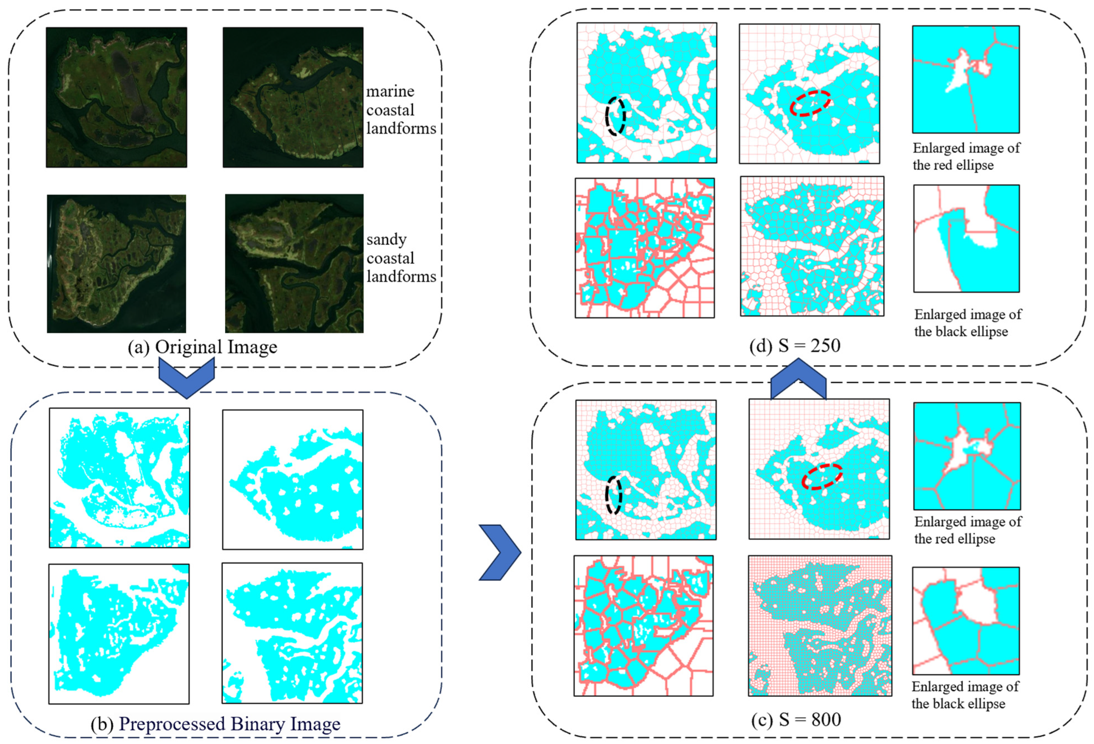
In this study, the remote sensing images used are high-resolution satellite images obtained through the Earth Online platform. Earth Online is an online platform dedicated to providing Earth observation data, bringing together image data from a variety of remote sensing satellites. These data not only have high spatial resolution but also provide multi-spectral information, allowing us to apply multiple spectral bands of information in detailed geomorphological analysis and texture migration work. The selected study area covers approximately 50 square kilometers in the Jonas Creek region of eastern Maryland, USA, which is located along the coast and belongs to the marine and sandy coastal landforms [36], as shown in Figure 2a. The top two images of Figure 2a are seafloor coastal landforms and the bottom two are sandy coastal landforms. This distinction between the sandy coastal landforms and marine landforms is crucial for our study, as it allows for a more focused examination of the interactions and representation of these specific coastal features in our multi-scale approach. The marine coastal landform includes winding rivers, extensive wetlands, and dense vegetation cover. These geomorphic features enrich the texture information of remote sensing images and provide differences in various surface reflectances, which are significant for the study of texture migration. In this environment, the complex vegetation structure and reflective features of the water make texture migration more challenging and also provide more layers of information. The sandy coastal landform is mainly composed of sand and sediment, showing distinct sand accumulation and erosion. In remote sensing images, these features appear as uniform and distinct textural features, such as smooth beach surfaces contrasting with rougher dunes. This geomorphic structure provides a regular target texture for texture migration, and the dynamic and seasonal changes of the sandy coast also add depth to the study.
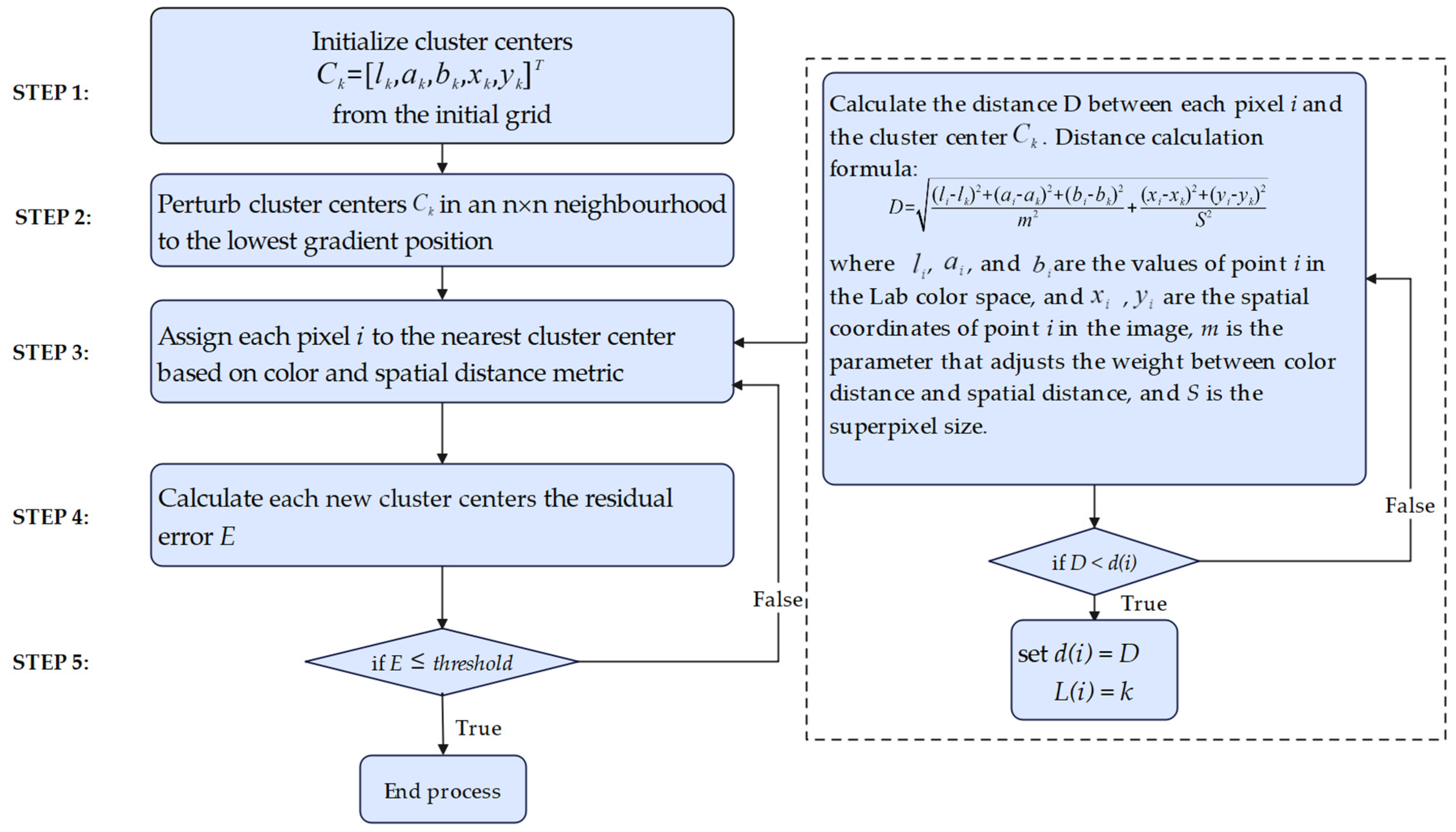
First, the original coastal landform image is preprocessed by converting it from RGB color space to Lab color space to better identify and distinguish different color regions, which improves the accuracy and precision of segmentation (Figure 2a,b). The Simple Linear Iterative Clustering (SLIC) [31] superpixel segmentation method is then applied to divide the image into smaller, homogeneous regions. SLIC is an efficient method for generating superpixels, as it clusters pixels based on their color and spatial proximity, using the Lab color space to ensure that color similarity plays a significant role in the clustering process. By minimizing the distance between pixels in both color and spatial dimensions, SLIC produces superpixels that respect image boundaries, making it highly suitable for complex coastal landform images. The flowchart of the specific SLIC is shown in Figure 3. The process begins with initializing cluster centers in the Lab color space, followed by assigning pixels to the nearest cluster center based on a combined metric of color and spatial distance. Each pixel is assigned to the cluster that minimizes this distance, ensuring both color and proximity are considered in the segmentation. After the initial assignment, cluster centers are updated by recalculating their positions based on the average color and spatial coordinates of the pixels assigned to them. This iterative process repeats until the cluster centers converge, producing superpixels that tightly align with the true boundaries of the image features. The number of superpixels can be adjusted, allowing for different levels of segmentation granularity, where a higher number of superpixels preserves more detail while fewer superpixels produce a coarser segmentation. Ultimately, the method ensures that important image details, especially in complex areas like coastal landforms, are well preserved, making it a powerful tool for image segmentation in scenarios where boundary precision is crucial.
Next, superpixel color clustering [32] is used to further group these superpixels based on color features. The number of superpixels (S) directly affects the results: a larger number of superpixels provides finer detail, while a smaller number results in coarser segmentation. For example, when S is reduced from 800 to 250, as shown in Figure 2c,d, the boundaries and features become less defined, leading to a loss of detail in the red and black ellipse areas. This highlights the trade-off between superpixel size and detail retention. Gradually reducing the number of superpixels can cause subtle changes and important details to be ignored or averaged, affecting the segmentation accuracy. The use of different levels of superpixel segmentation enables more comprehensive feature extraction and improves the segmentation results by allowing for multi-scale analysis (Figure 2c,d).

3.2. Coastal Landform Simplification and Global Aggregation

After the original coastal landform image is segmented by the SLIC algorithm, to describe and understand the structure and attributes of these superpixels more accurately, the segmented superpixels are divided into six categories. This approach aligns with Tobler’s First Law of Geography [37], which states that “everything is related to everything else, but near things are more related than distant things”. In this context, superpixels represent regions of spatial proximity and similarity, reflecting geographic relationships in the image.
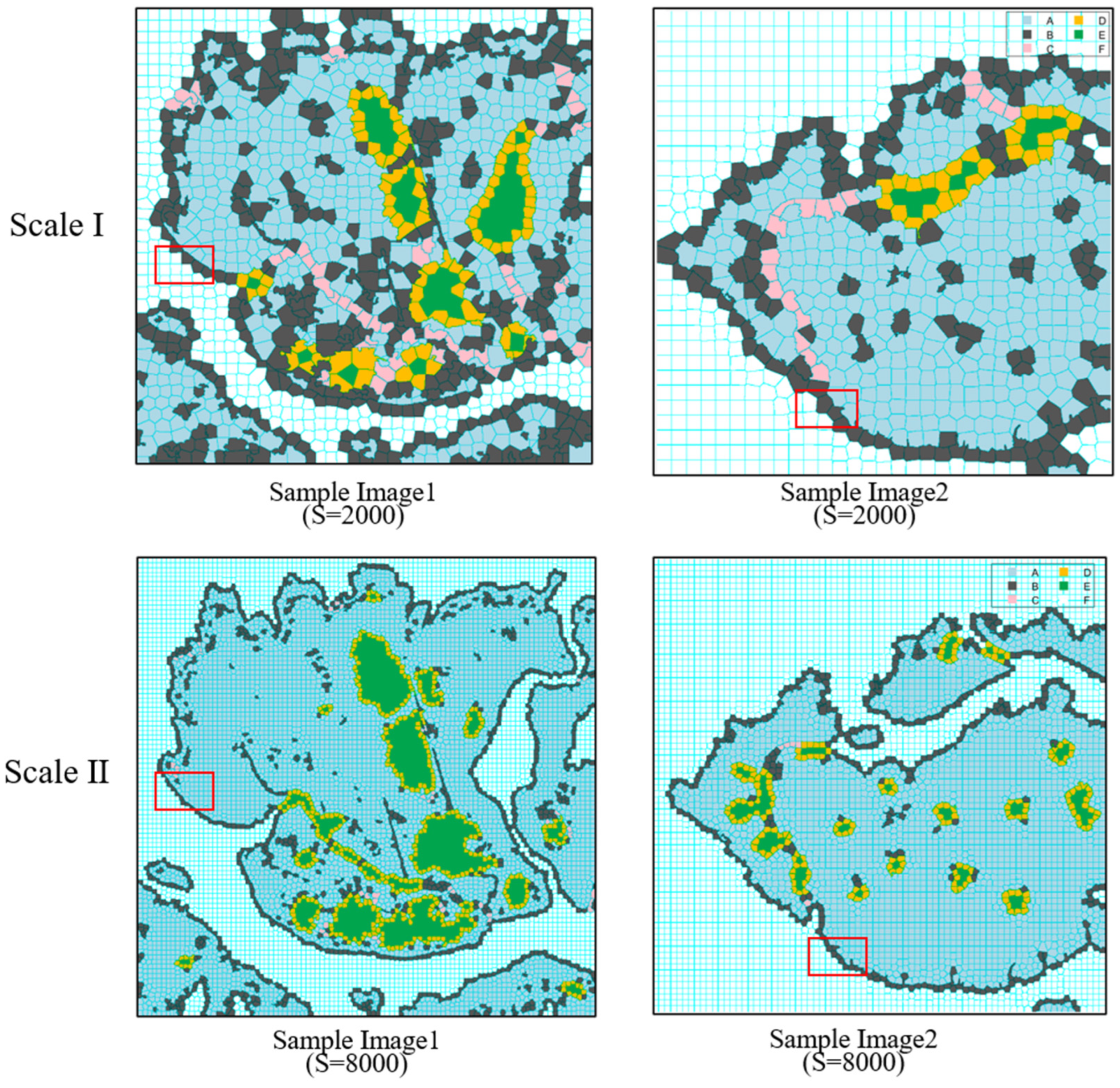
Specifically, Sample Image 1 with S = 2000 is selected as a case study to analyze the classification rules, as illustrated in Figure 4. For a clearer comparison, images from the same area are divided into two scales: Scale I and Scale II, which correspond to different numbers of superpixels. Scale I, with fewer superpixels, smooths boundaries, as seen in the red box where previously jagged hyperpixelated borders become more circular. In contrast, Scale II contains more superpixels, preserving finer boundary details and highlighting the spatial correlation between nearby regions.
Tobler’s law reinforces the idea that geographic objects, like the superpixels in Scale II, should maintain more precise boundaries because closer regions exhibit stronger relationships. The scale difference illustrates that while global features are enhanced in Scale I, the local precision in Scale II provides a clearer understanding of boundary details and spatial structure, essential for multi-scale geographic feature classification and analysis.
Therefore, the global aggregation of superpixel-segmented coastal landforms goes through the following steps: Firstly, in the first step, the image of the region is segmented into superpixels. In the second step, the segmented superpixels are classified into six categories according to their connectivity and geometric relationships [18]: Class A superpixels, which make up most of the underlying area-like features, cover most of the terrain in the figure. This class of superpixels represents the base part of the coastline and other widely distributed geographic units. The light blue superpixels are shown in Figure 4: the second class, Class B superpixels, are mainly concentrated at the outer edge of Class A superpixels and are scattered. Shown in Figure 4 as a dark gray superpixel, the third category, class C superpixels, are adjacent to class A superpixels but connected to two or more polygons, which play the role of connecting different regions and represent geographic units with transition characteristics. The pink superpixel shown in Figure 4, the fourth class, class D superpixels, have regular and closed morphology, forming relatively independent small areas and presenting obvious embedded structures, as shown in the yellow superpixels in Figure 4. The fifth category, the nested regions of class E superpixels and class D superpixels, have closed or nearly closed shapes and represent more independent geographical units, as shown in the green superpixels in Figure 4. The sixth class, class F superpixels, and all other superpixels except the above five classes are class F superpixels, as shown by the white superpixels in Figure 4. In the third step, smoothing and merging regions are generated, and superpixels of classes A, B, C, and D are selected as regions to be merged to form a larger region representing coastal geomorphic features. A median filtering technique is used on the edges of these regions to obtain smooth merged regions. Through these steps, superpixels are merged to form a globally simplified and coherent representation of the coastal landform, ensuring that the main features of the coastal landform are clearly delineated and smoothed.
After global aggregation, we find that there are still two problems. The first is that as the number of superpixels gradually decreases, the distance between the globally merged boundary and the original image boundary increases, as shown in Figure 4. The second is that as the number of superpixels gradually decreases, the boundary after global simplification becomes less and less smooth, which is not conducive to maintaining the global features of the image and realizing global merging through texture migration.
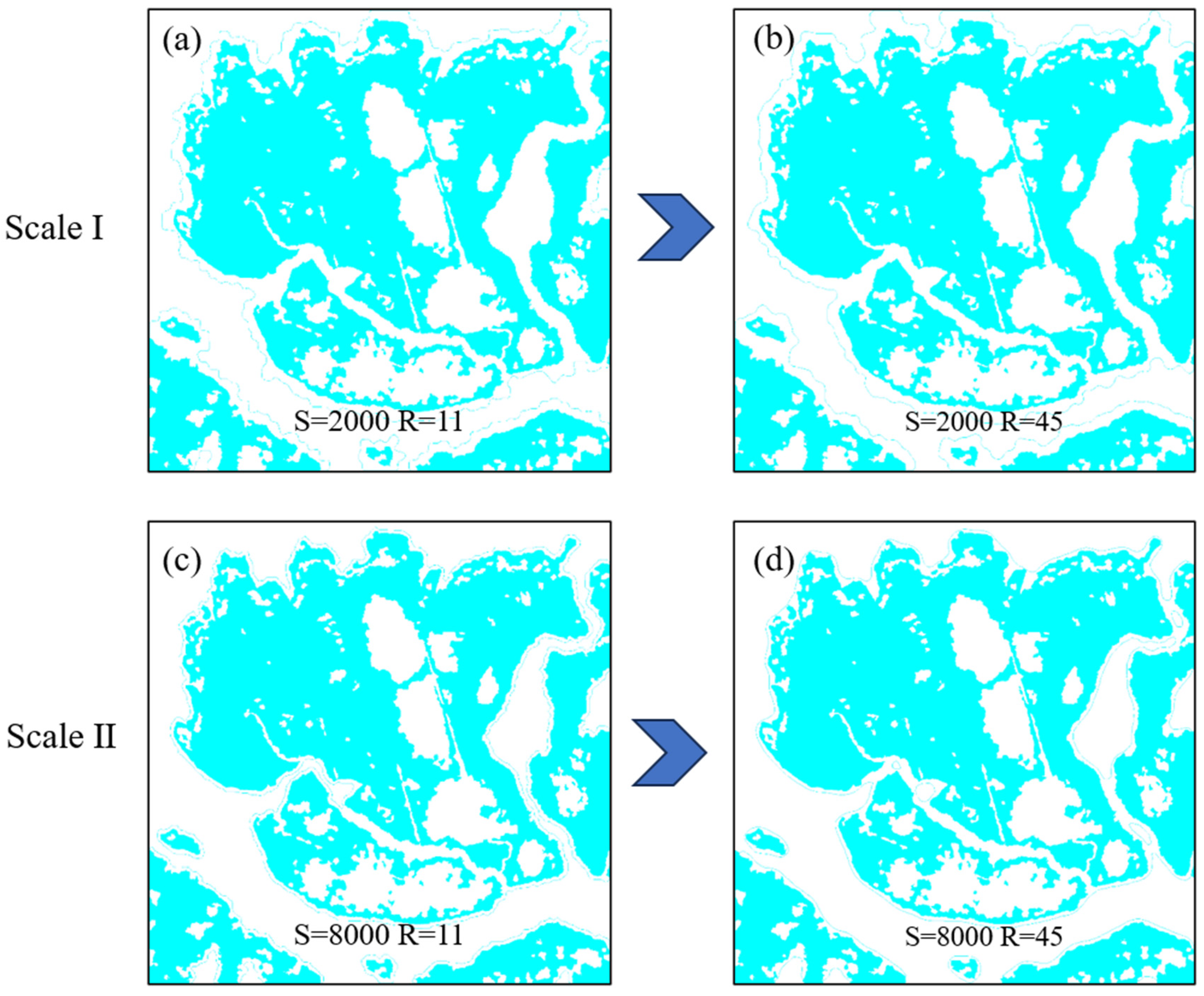
To solve the first problem, we introduce the two basic operators of mathematical morphology, namely, expansion and corrosion [38], to further adjust the boundary of the superpixel and make it better match the boundary of the original image. The combined superpixel is expanded to make its boundary expand outward by a certain distance. Then, the expanded superpixel is corroded to make its boundary shrink inward by a certain distance. For the second problem, we first detect the edges in the image by using the Sobel edge detection algorithm [39]. The Sobel edge detection algorithm locates the edges by calculating the gradient of image pixels in the horizontal and vertical directions and can detect the edges simply and effectively. Then, the four classes of superpixels (A, B, C, and D) are smoothed by the edge median filtering. The median filtering replaces the value of the center pixel with the median value of the pixel in the window, which can effectively reduce the influence of noise while preserving the edge information of the image. Figure 5a–d show the effect of global simplification with a filtering kernel of size. We consider the reconstruction results of the original boundary of the filtering kernel R = 11 and R = 45 at different superpixel sizes. Figure 5a,b display that when S is unchanged, the information of the boundary is gradually removed and the uneven smoothness is gradually reduced with the continuous increase of R value. Under different levels, with the continuous increase of S, the smoothness of the boundary is significantly enhanced, and the distance between the generated boundary and the original image boundary becomes smaller. When R is constant, with the increasing of S, the region generated by the boundary increases, and more holes can also be generated. In other words, the final global features of coastal landform superpixels are determined by S and R together (Figure 5a,c). For complex geomorphic features such as the Mediterranean landform, a higher S value, such as S = 8000, can be selected to capture more details and features, and generate more merging areas to maintain the global characteristics of the marine coastal landform. A larger filtering kernel ensures the smoothness of the boundary and the effective reduction of noise; in this example, R = 45 can be selected (Figure 5d).

3.3. Texture Transfer of the Merged Coastal Landform

We need to carry out texture transfer on the result of global simplification to preserve the texture characteristics of coastal landforms. Texture transfer [35] is an image processing technique that applies the texture of one image to another, allowing the target image to achieve a similar texture effect without altering its overall structure and content, thus achieving better aggregation effects [40]. Figure 6 shows the migration process. The key step in texture transfer is to create a mask of the same size as the input image, which is shown in the middle of Figure 6. We divide the mask creation process into four steps. Step 1 simplifies and merges the original image to generate the boundary. Step 2 converts the original image into a black-and-white binary image using the RGB color channel for ease of mask generation. Step 3 uses the Sobel edge detection algorithm to fill the boundary generated by image simplification, turning the filled part black and the remaining part white for uniform coloring. Step 4 involves subtracting the black regions in image (b) from those in image (a), turning the result white, which represents the area where the texture will be migrated, with the rest remaining black. In the specific processing steps, we compare three different texture transfer algorithms, including the image inpainting technique based on the Fast Marching Method (FMM) [41] developed by Alexandru, the image inpainting algorithm based on the Navier–Stokes equation (NS) [42], and the Non-Local Means (NL-Means) [43] inpainting algorithm. The FMM algorithm was based on the numerical solution of the wave equation and filled the missing area by following the advanced path of the wave. This method started with a known pixel value and continued to expand outward, simulating the way fluctuations propagate, and was able to handle the restoration of continuous and natural images well, producing smooth and natural results. In the repair process, the algorithm first filled the boundary pixels of the region, then selected a small neighborhood around the pixel to be repaired, used normalized weighting, and updated the value of the pixel to be repaired. The NS algorithm was based on fluid dynamics and partial differential equations. The basic principle was heuristics. Formula (1) represents the calculation process of the NS algorithm, which first accesses from the known region along the edge to the unknown region (since the edge should be continuous). It continues to draw contours (lines connecting points of the same brightness, similar to contour lines) while matching the gradient vector of the boundary of the area to be repaired. Then fills in the missing parts of the image naturally and retains the edge and detailed information in the image.
          ρ u t + ρ u · u = p + μ 2 u + F
In this formula, ρ represents the fluid density, u is the velocity vector, p is the pressure, μ is the dynamic viscosity, F is the shear force acting on the fluid per unit mass, ∇ is the gradient operator, and ∇2 is the Laplacian operator.
Non-Local Means (NL-Means) is an algorithm for image denoising and repairing, its core idea is to use similar local areas in the image to repair or denoise. Unlike traditional local averaging methods, NL-Means searches all the pixels in an image and finds pixels that are similar to those to be repaired or denoised, then weights those similar pixels [44]. This process takes into account the non-local information of the image and thus allows for better preservation of image detail and texture.
In order to select an appropriate and accurate image restoration algorithm for texture migration, we comprehensively evaluate the MSE, PSNR, NMI, and SSIM [45,46] of the three texture migration results in Figure 6 and the original image, and output, and present the results in Table 1.
Mean square error (MSE) is a standard measure of the quality of an image reconstruction or restoration. It evaluates the difference between images by squaring and averaging the difference between image pixel values; the smaller the MSE value, the more similar the two images are [44]. The formula for MSE is as follows, where I i , j and K ( i , j ) are the pixel values of the original and reconstructed images, respectively, and mmm and nnn are the dimensions of the images.
M S E = 1 m n i = 1 m j = 1 n ( I i , j K ( i , j ) ) 2
Peak signal-to-noise ratio (PSNR) is a measure of image quality, representing the peak signal-to-noise ratio of image reconstruction quality. The larger the PSNR value, the better the image reconstruction quality. It is calculated using the following formula:
P S N R = 10 l o g 10 ( L 2 M S E )
Normalized Mutual Information (NMI) is an information theory measure used to evaluate the similarity of two images. The NMI value is between 0 and 1, and the larger the value, the more similar the two images are. The NMI value is calculated as
N M I ( A , B ) = 2 I ( A , B ) H A + H ( B )
where I ( A , B ) is the mutual information between images A and B, and H A and H ( B ) are the entropies of images A and B.
Structural Similarity Index (SSIM) is a measure of structural similarity between two images, taking into account image brightness, contrast, and structural information [44]. The SSIM value is between 0 and 1, and the closer the value is to 1, the more similar the structure of the two images is.
S S I M x , y = ( 2 μ x μ y + C 1 ) ( 2 σ x y + C 2 ) ( μ x 2 + μ y 2 + C 1 ) ( σ x 2 + σ y 2 + C 2 )
where μ x and   μ y are the means of images x and y, σ x 2 and σ y 2 are the variances, σ x y is the covariance, and C 1 and C 2   are constants to avoid instability.
As can be seen from Table 1, the MSE value of the NL-Means method (28.676) is significantly higher than that of the FMM and NS methods, which indicates that the NL-Means method has poor image restoration quality in the MSE measurement. However, the image repair effect of the NS method is slightly better than that of the FMM. On PSNR, the NS method has the best image repair effect, which is slightly better than the FMM. On the NMI measure, FMM (0.261), NS (0.2584), and NL-Means (0.2548) are nearly equal, indicating little difference in performance between the three methods. The three methods have little difference in their SSIM measurements. On the whole, the NS method has the best performance in MSE and PSNR indicators, so in terms of minimizing pixel error, maximizing signal-to-noise ratio, and maintaining texture features, the NS method is the best choice. Therefore, we will use the NS algorithm to migrate the texture of the globally merged image.

4. Experiment—A Case Study of Coastal Landform Aggregation

4.1. Experimental Data

In this experiment, the coastal geomorphology data used to test the algorithm come from the remote sensing map of satellites on Earth Online. We can download these tile data free of charge from the official website, as shown in Figure 7. We can see the overview map of the study area in Figure 7g. The coastal geomorphic data used in this experiment were collected from the marine and sandy coastal geomorphic areas near Jones Beach, New York City, USA. Among them, the sandy coastal landforms of (a–c) are mainly composed of loose sand, gravel, and other granular materials. The continuous accumulation of waves forms a broad beach and coastal sand embankment. The latitude and longitude of the central point of the region is 41.5331°N, 71.8202°W. And the coastal landform of marine sediment of (d–f) is a typical Marine sediment landform area with abundant topographic and textural features. The latitude and longitude of the central point of this region are 40.5883°N, 73.5023°W, which is very suitable for the study of merging and texture migration in multi-scale expression. The study area is composed of 200 tiles, each with a resolution of 256 × 256 pixels. The downloaded tile data are spliced to form a complete landform image.

4.2. Experimental Process

In the first step of the METF-C method, feature extraction is carried out on the original marine sediment coast geomorphic data and the original sandy coast geomorphic data. Four sample graphs are selected in two experimental areas for experiments. The feature extraction results are shown in Figure 8. The sandy coast landform is shown in Sample Images 1 and 2, and the marine sediment coast landform is shown in Sample Images 3 and 4. The upper right corners of the last two columns show the enlarged boundaries of various examples under different superpixels. As scale S increases, comparing Figure 8(c1,d1), the boundary of the hole within the red box in c1 is not recognized, and boundary details are missing. In contrast, d1 shows a clearer segmentation and clustering result with better boundary detail recognition. Comparing Figure 8(c2,d2), although the boundary within the red box in c2 is recognized, the result is not satisfactory. d2 aligns more closely with the original image boundaries and effectively captures boundary details. Similarly, in comparing Figure 8(c3,d3), c3 fails to recognize the boundary of the hole within the box, whereas d3 successfully identifies the hole boundary. Lastly, comparing Figure 8(c4,d4), c4 identifies the boundary of the hole, but the boundary is quite distant from the original image boundaries and does not match the original features well. Conversely, d4 effectively captures the hole boundary. Therefore, under the multi-scale study of the METF-C method, a scale of S = 800 is more advantageous for preserving the boundary features of the original image (Figure 8(a1–d4)).
Then, the second step of the METF-C method is carried out to simplify and merge the experimental data globally. In order to better demonstrate the advantages of the METF-C method, we introduce the merge operation in ArcGIS for comparison. The aggregation parameter settings for METF-C and ArcGIS are shown in Table 2. For the METF-C method, the number of superpixels (S) reflects the scale at which the method operates, controlling how fine or coarse the segmentation is [32]. At level I, S is set to 2500, which results in larger superpixels and a broader simplification of the data. The filter kernel radius (R), which influences the smoothing and aggregation of superpixels, is set to 45 for level I. As we move to level II, S increases to 12,500, indicating a finer scale with smaller superpixels, while the filter kernel radius R is reduced to 11 to maintain finer boundary details. This adjustment of S and R allows the METF-C method to adapt to different scales of analysis, ensuring that critical features are preserved while simplifying less relevant details.
In contrast, the ArcGIS method, which operates on vector data rather than raster data, does not use superpixel-based parameters such as S or R. Instead, the ArcGIS method relies on the aggregation distance to determine how features are merged [47]. At level I, the aggregation distance is set to 100 m, which facilitates broader merging of features. At level II, the aggregation distance increases to 150 m, allowing for more detailed feature retention as compared to level I. This parameter setting provides a flexible way to control the scale of aggregation, though it may lack the finer control over spatial data smoothing provided by the METF-C method. The combined parameters of the two methods are shown in the table, where the symbol “-” indicates that the corresponding algorithm does not set a value for the parameter.
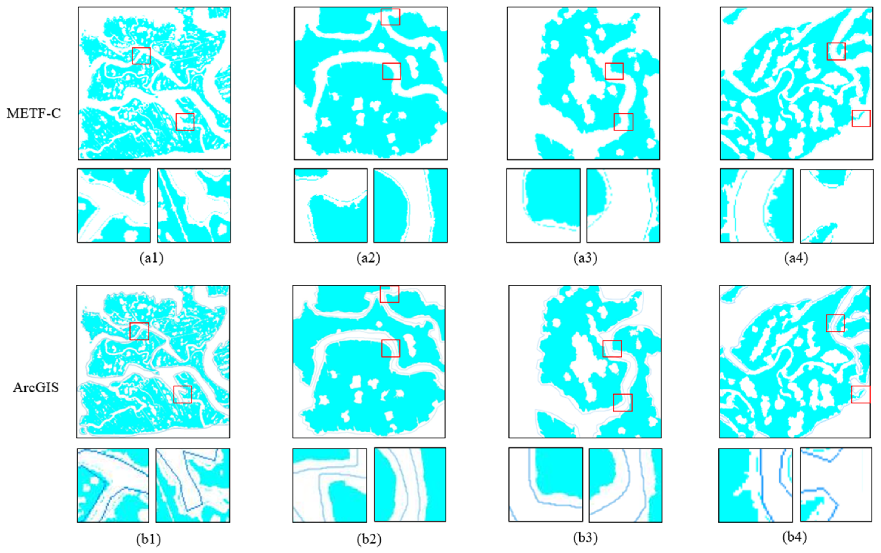
Figure 9 illustrates the results of two different merging methods, providing a detailed comparison by showing enlarged views of the boundaries within the red boxes beneath each merging result. When comparing the merging boundaries generated by the ArcGIS method (Figure 9(b1–b4)) with those from the METF-C method (Figure 9(a1–a4)), it becomes evident that the boundaries produced by the METF-C method are closer to the original binary image boundaries. This difference is particularly noticeable in images a3 and b3, where the METF-C method demonstrates a clear advantage in terms of boundary precision. Specifically, the METF-C method achieves more accurate boundary lines with a smaller distance from the original binary boundaries, highlighting its strength in maintaining boundary integrity and precision during the merging process. In contrast, the ArcGIS method, which relies on vector boundary synthesis, produces boundaries that, while efficiently generated, tend to be less smooth, exhibiting some degree of irregularity and jagged edges. These irregularities can negatively impact subsequent processes like texture migration, leading to less natural and less smooth final results. On the other hand, the METF-C method, by generating smoother and more continuous boundary lines, ensures that the texture migration process results in more natural boundary transitions, ultimately achieving a more desirable and realistic outcome. Figure 10 presents the results of texture migration using these merged and simplified images. The a1 and b1 images depict marine sedimentary coastal landforms, while images c1 and c3 represent sandy coastal landforms.

4.3. Comparison and Analysis of Experimental Results

In order to qualitatively evaluate the METF-C method, traditional multi-scale representation methods, including median filtering, image pyramid, and Gaussian filtering, were used to compare the results. The corresponding parameter settings include the kernel size, scale factor, and sigma [48,49,50,51] of the METF-C method, median filtering, image pyramid, and Gaussian filtering at two levels and are shown in Table 3, and the specific results are shown in Figure 11. Image filtering [10] and image pyramid [11] methods can smooth and compress image content, so they are widely used in multi-scale image representation [52].
By comparing the three traditional methods with the METF-C method, it can be found that the METF-C method has the following advantages:
First, as shown in the area marked by the green circle in Figure 11a, although the median filtering method can smooth the shape of coastal landforms to a certain extent, it will lead to distortion of remote sensing image content. With the shrinking of the image size, the contents of the remote sensing image of the original coastal landform, including the boundary features, are almost completely unreadable. In addition, the texture features of the sandy coastal landform in Figure 10b are becoming more and more blurred, and the original texture cannot be maintained. Compared with the area marked by the white circle in Figure 11a, the METF-C method can not only effectively retain the key boundary features of the coastal landform, but also relatively maintain the original texture of the coastal landform in multi-scale changes, thus avoiding the distortion problem caused by the median filtering method.
Second, as shown in the areas marked with orange and white circles in Figure 11a, both the METF-C method and the image pyramid method proposed in this paper can maintain the clarity of the image when the size of the image is reduced. However, the image pyramid method is not good at simplifying the boundary of coastal landforms in remote sensing images and cannot reduce the boundary complexity of coastal landforms, so it cannot reduce the visual burden. In contrast, the METF-C method can not only maintain the clarity of the image but also effectively simplify the complexity of the coastal geomorphic boundary and maintain the original texture features of the image in the multi-scale process. This enables METF-C to better balance the needs of texture detail preservation and boundary simplification when processing high-resolution remote sensing images and have a better performance than the image pyramid method.
Third, as shown in the area marked by the blue circle in Figure 11a, although the Gaussian filtering method can smooth the noise to a certain extent in the multi-resolution expression of remote sensing images, it is poor in maintaining the clarity and legibility of lake information, resulting in difficulty in identifying and understanding the morphological characteristics of lake boundaries. In the process of multi-scale expression, the METF-C method can not only effectively simplify the complexity of lake boundaries but also maintain a high level of clarity and information integrity, so that it is superior to the Gaussian filtering method in visual presentation and information expression.
Figure 11b shows the comparison of results of the median filtering, Gaussian filtering, image pyramid, and METF-C methods in the multi-scale representation of sandy coastal landforms, and it can be seen that their features are similar. Through these comparisons, we can see the advantages of the METF-C method in multi-scale image expression.
To quantitatively evaluate the proposed METF-C method, lake images processed using METF-C were compared with the results of other multi-scale image processing methods, including image filtering, image pyramid, and median filtering. The performance of these methods was assessed using three key metrics: Edge Preservation Index (EPI), Texture Clarity Score (TCS), and Information Retention Rate (IRR). These metrics were calculated for each of the four methods at two different scales (Scale I and Scale II).
The Edge Preservation Index (EPI) measures the sharpness of boundaries after image processing. It evaluates edge preservation by calculating the edge similarity between the original and processed images. The Structural Similarity Index (SSIM) or other edge detection methods are used to assess this similarity. An EPI value closer to 1 indicates better edge preservation. The Texture Clarity Score (TCS) assesses how well the texture details are preserved in an image. It is typically calculated by determining the local variance of the image or via frequency domain analysis. A higher TCS value signifies that more texture details are retained after processing. The Information Retention Rate (IRR) quantifies the degree of information retained in the image after processing. It is measured by comparing the entropy of the image before and after processing. An IRR value closer to 1 indicates that the processed image closely retains the information of the original image, implying minimal information loss.
Table 4 presents the EPI, TCS, and IRR results for METF-C, median filtering, image pyramid, and Gaussian filtering across two scales. It can be found from the table that, firstly, in terms of edge preservation, the METF-C method has the strongest edge preservation ability under two scales. Especially under Scale I, the Edge Preservation Index reaches 0.988, which indicates that it can still preserve the image boundary well after processing. Secondly, in terms of texture preservation, although the texture preservation ability of the image pyramid method is slightly better than that of METF-C under Scale I, the METF-C performs well under Scale II and can better preserve texture details under multi-scale conditions. Finally, in terms of information retention, METF-C has the best Information Retention Rate in both scales, indicating that it loses the least information in the processing process and can retain the information of the original image to the maximum extent.

5. Conclusions

The multi-scale expression of remote sensing images provides important data support and analysis tools for various applications and plays an important role in many fields. By combining superpixel segmentation and texture transfer techniques, this paper proposes a new multi-scale expression method for coastal landforms in remote sensing images (METF-C) to overcome the shortcomings of traditional methods in processing complex texture features and rich color images. In this method, superpixel segmentation is used to achieve fine segmentation of geomorphic elements, and rule selection and median filtering are used to smooth boundary adjustments, and finally, texture transfer is used to achieve multi-scale and multi-level coastal landform combined images. Compared with the traditional remote sensing image multi-scale expression technology, this paper has the following advantages:
(1)
The METF-C method uses superpixel segmentation technology to achieve fine segmentation of geomorphic elements, thereby improving the resolution and accuracy of the image and making the combined image clearer and more accurate;
(2)
The traditional method has limitations in processing complex texture features and colorful images [53], while the METF-C method effectively maintains the texture features of the original landform through texture transfer technology, making the combined image more realistic and accurate in texture;
(3)
The traditional method cannot effectively maintain the global features of images at the multi-scale level [54], while the METF-C method combines the technology of superpixel segmentation and rule selection, which can realize the combination of landform images with multiple scales and levels and effectively retain the global features of images.
However, the METF-C method still has the following limitations in the multi-scale expression of remote sensing images. First of all, in multi-scale expression, this method mainly aims at the multi-scale expression of coastal geomorphology, which may not be effective in areas with drastic geomorphological changes. If the landform changes greatly, the texture transfer results may not be ideal, thus affecting the final aggregation effect. Secondly, this method takes into account the texture features of coastal landforms, and its applicability is limited by specific geographical scenarios and application fields and may not be suitable for other application scenarios.

Author Contributions

Conceptualization, R.Z. and Y.S.; methodology, R.Z.; software, Y.S.; validation, R.Z. and Y.S.; formal analysis, Y.S.; investigation, R.Z.; resources, Y.S.; data curation, R.Z.; writing—original draft preparation, R.Z.; writing—review and editing, Y.S.; visualization, R.Z.; supervision, Y.S.; project administration, R.Z. and Y.S.; funding acquisition, Y.S. All authors have read and agreed to the published version of the manuscript.

Funding

This work was supported by the research startup fund at Sun Yat-sen University.

Data Availability Statement

The data presented in this study are openly available in https://www.earthol.com.

Conflicts of Interest

The authors declare no conflicts of interest.

References

  1. Dollár, P.; Appel, R.; Belongie, S.; Perona, P. Fast Feature Pyramids for Object Detection. IEEE Trans. Pattern Anal. Mach. Intell. 2014, 36, 1532–1545. [Google Scholar] [CrossRef]
  2. Hay, G.J.; Blaschke, T.; Marceau, D.J.; Bouchard, A. A Comparison of Three Image-Object Methods for the Multiscale Analysis of Landscape Structure. ISPRS J. Photogramm. Remote Sens. 2003, 57, 327–345. [Google Scholar] [CrossRef]
  3. Zou, Z.; Chen, K.; Shi, Z.; Guo, Y.; Ye, J. Object Detection in 20 Years: A Survey. Proc. IEEE 2023, 111, 257–276. [Google Scholar] [CrossRef]
  4. Sedaghat, A.; Mokhtarzade, M.; Ebadi, H. Uniform Robust Scale-Invariant Feature Matching for Optical Remote Sensing Images. IEEE Trans. Geosci. Remote Sens. 2011, 49, 4516–4527. [Google Scholar] [CrossRef]
  5. Irons, J.R.; Petersen, G.W. Texture Transforms of Remote Sensing Data. Remote Sens. Environ. 1981, 11, 359–370. [Google Scholar] [CrossRef]
  6. Fernandez-Beltran, R.; Haut, J.M.; Paoletti, M.E.; Plaza, J.; Plaza, A.; Pla, F. Remote Sensing Image Fusion Using Hierarchical Multimodal Probabilistic Latent Semantic Analysis. IEEE J. Sel. Top. Appl. Earth Obs. Remote Sens. 2018, 11, 4982–4993. [Google Scholar] [CrossRef]
  7. Ben Hamza, A.; He, Y.; Krim, H.; Willsky, A. A Multiscale Approach to Pixel-Level Image Fusion. Integr. Comput.-Aided Eng. 2005, 12, 135–146. [Google Scholar] [CrossRef]
  8. Teodoro, A.C.; Pais-Barbosa, J.; Veloso-Gomes, F.; Taveira-Pinto, F. Evaluation of Beach Hydromorphological Behaviour and Classification Using Image Classification Techniques. J. Coast. Res. 2009, II, 1607–1611. [Google Scholar] [CrossRef]
  9. Wu, D.; Shen, Y.; Fang, R. Morphological Change Characteristics of Tidal Gullies in Central Jiangsu Coast. Acta Geograph. Sin. 2013, 68, 955–965. [Google Scholar]
  10. Tang, K.; Astola, J.; Neuvo, Y. Nonlinear Multivariate Image Filtering Techniques. IEEE Trans. Image Process. 1995, 4, 788–798. [Google Scholar] [CrossRef]
  11. Gluckman, J. Scale Variant Image Pyramids. In Proceedings of the IEEE Computer Society Conference on Computer Vision and Pattern Recognition (CVPR), New York, NY, USA, 17–22 June 2006; pp. 1069–1075. [Google Scholar] [CrossRef]
  12. Gonzalez, R.C.; Woods, R.E. Digital Image Processing; Prentice Hall: Upper Saddle River, NJ, USA, 2008; pp. 165–170. [Google Scholar]
  13. Wei, G.; Yang, J.; Zhang, H. Comparative Study of Commonly Used Nonlinear Filtering Methods. Electro-Optics Control 2009, 16, 48–52. [Google Scholar]
  14. Arulampalam, M.S.; Maskell, S.; Gordon, N.; Clapp, T. A Tutorial on Particle Filters for Online Nonlinear/Non-Gaussian Bayesian Tracking. IEEE Trans. Signal Process. 2002, 50, 174–188. [Google Scholar] [CrossRef]
  15. Smith, S.M.; Brady, J.M. SUSAN—A New Approach to Low Level Image Processing. IEEE Trans. Pattern Anal. Mach. Intell. 1997, 21, 443–456. [Google Scholar] [CrossRef]
  16. Burt, P.; Adelson, E. The Laplacian Pyramid as a Compact Image Code. IEEE Trans. Commun. 1983, 31, 532–540. [Google Scholar] [CrossRef]
  17. Usui, H. Automatic Measurement of Building Setbacks and Streetscape Widths and Their Spatial Variability Along Streets and in Plots: Integration of Streetscape Skeletons and Plot Geometry. Int. J. Geogr. Inf. Sci. 2023, 37, 810–838. [Google Scholar] [CrossRef]
  18. Shen, Y.; Ai, T.; Li, W.; Wu, L. A Polygon Aggregation Method with Global Feature Preservation Using Superpixel Segmentation. Comput. Environ. Urban Syst. 2019, 75, 117–131. [Google Scholar] [CrossRef]
  19. Hermosilla, T.; Ruiz, L.A.; Recio, J.A.; Estornell, J. Assessing Contextual Descriptive Features for Plot-Based Classification of Urban Areas. Landsc. Urban Plan. 2012, 106, 124–137. [Google Scholar] [CrossRef]
  20. Burger, P.R. Exploring Geographic Information Systems (Book Review). Geogr. Bull. 1998, 40, 59. [Google Scholar]
  21. Fairclough, H.; Gilbert, M. Layout Optimization of Simplified Trusses Using Mixed Integer Linear Programming with Runtime Generation of Constraints. Struct. Multidiscip. Optim. 2020, 61, 1977–1999. [Google Scholar] [CrossRef]
  22. Peng, D.; Wolff, A.; Haunert, J.H. Finding Optimal Sequences for Area Aggregation—A* vs. Integer Linear Programming. ACM Trans. Spat. Algorithms Syst. (TSAS) 2020, 7, 1–40. [Google Scholar] [CrossRef]
  23. Wang, Z.; Liu, Y.; Zhang, H. Coastal Line Simplification Based on Fuzzy Logic. IEEE Trans. Geosci. Remote Sens. 2018, 56, 5015–5027. [Google Scholar] [CrossRef]
  24. Li, X.; Zhao, Q. Multi-Scale Analysis of Coastal Landforms Using Feature Extraction Techniques. IEEE Trans. Geosci. Remote Sens. 2019, 57, 1698–1710. [Google Scholar] [CrossRef]
  25. Chen, L.; Xu, J.; Wang, Y. Automatic Coastal Landform Merging Using Convolutional Neural Networks. IEEE J. Sel. Top. Appl. Earth Obs. Remote Sens. 2021, 14, 5307–5318. [Google Scholar] [CrossRef]
  26. McMaster, R.B. A Conceptual Model of the Interaction between Simplification and Smoothing. Cartogr. J. 1986, 23, 27–34. [Google Scholar]
  27. Buchin, K.; van Kreveld, M.; Löffler, M.; Luo, J.; Silveira, R.I.; Wolff, A. Simplifying a Polygonal Subdivision While Keeping It Simple. Comput. Geom. 2011, 44, 435–446. [Google Scholar] [CrossRef]
  28. Tong, X.; Shi, W. A Scale-Adaptive Model for the Simplification of Areal Features. Int. J. Geogr. Inf. Sci. 2002, 16, 323–343. [Google Scholar] [CrossRef]
  29. Gong, J.; Zhao, S.; Liu, Y.; Li, M. Multi-Resolution Terrain Simplification and Visualization Based on Triangulated Irregular Networks. Remote Sens. 2013, 5, 5447–5463. [Google Scholar] [CrossRef]
  30. French, J.; Payo, A.; Murray, B.; Orford, J.; Eliot, M.; Cowell, P. Appropriate Complexity for the Prediction of Coastal and Estuarine Geomorphic Behaviour at Decadal to Centennial Scales. Geomorphology 2016, 256, 3–16. [Google Scholar] [CrossRef]
  31. Liu, Y.J.; Yu, C.C.; Yu, M.J.; Su, D. Manifold SLIC: A Fast Method to Compute Content-Sensitive Superpixels. In Proceedings of the IEEE Conference on Computer Vision and Pattern Recognition (CVPR), Las Vegas, NV, USA, 27–30 June 2016; pp. 651–659. [Google Scholar] [CrossRef]
  32. Achanta, R.; Shaji, A.; Smith, K.; Lucchi, A.; Fua, P.; Süsstrunk, S. SLIC Superpixels Compared to State-of-the-Art Superpixel Methods. IEEE Trans. Pattern Anal. Mach. Intell. 2012, 34, 2274–2282. [Google Scholar] [CrossRef]
  33. Villar, S.A.; Torcida, S.; Acosta, G.G. Median Filtering: A New Insight. J. Math. Imaging Vis. 2017, 58, 130–146. [Google Scholar] [CrossRef]
  34. Raid, A.M.; Khedr, W.; El-Dosuky, M.; El-Bassiouny, A. Image Restoration Based on Morphological Operations. Int. J. Comput. Sci. Eng. Inf. Technol. 2014, 4, 9–21. [Google Scholar] [CrossRef]
  35. Wang, Z.; Zhao, L.; Chen, H.; Lu, S. Texture Reformer: Towards Fast and Universal Interactive Texture Transfer. In Proceedings of the AAAI Conference on Artificial Intelligence, Vancouver, BC, Canada, 22 February–1 March 2022; pp. 2624–2632. [Google Scholar] [CrossRef]
  36. McGill, J.T. Map of Coastal Landforms of the World. Geogr. Rev. 1958, 48, 402–405. [Google Scholar] [CrossRef]
  37. Tobler, W. A computer movie simulating urban growth in the Detroit region. Econ. Geogr. 1970, 46, 234–240. [Google Scholar] [CrossRef]
  38. Harsimran, S.; Santosh, K.; Rakesh, K. Overview of Corrosion and Its Control: A Critical Review. Proc. Eng. Sci. 2021, 3, 13–24. [Google Scholar] [CrossRef]
  39. Zhang, Q.; Li, L.; Wang, H. Sobel Edge Detection Based on Weighted Nuclear Norm Minimization Image Denoising. Appl. Sci. 2023, 12, 120–130. [Google Scholar] [CrossRef]
  40. Zhang, Z.; Wang, Z.; Lin, Z.; Qi, H.; Wang, L.; Yang, Y. Image Super-Resolution by Neural Texture Transfer. In Proceedings of the IEEE/CVF Conference on Computer Vision and Pattern Recognition (CVPR), Long Beach, CA, USA, 16–20 June 2019; pp. 7982–7991. [Google Scholar]
  41. Wang, Z.; Wang, Q.; Moran, B.; Xia, Y.; Ha, L. Optimal Submarine Cable Path Planning and Trunk-and-Branch Tree Network Topology Design. IEEE/ACM Trans. Netw. 2020, 28, 1562–1572. [Google Scholar] [CrossRef]
  42. Radhakrishnan, R. A Survey of Multiscale Modeling: Foundations, Historical Milestones, Current Status, and Future Prospects. AIChE J. 2021, 67, e17026. [Google Scholar] [CrossRef]
  43. Zhang, X. Two-Step Non-Local Means Method for Image Denoising. Multidimens. Syst. Signal Process. 2022, 33, 341–366. [Google Scholar] [CrossRef]
  44. Liu, Y.L.; Wang, J.; Chen, X.; Li, W.; Xu, M. A Robust and Fast Non-Local Means Algorithm for Image Denoising. J. Comput. Sci. Technol. 2008, 23, 270–279. [Google Scholar] [CrossRef]
  45. Köksoy, O. Multiresponse Robust Design: Mean Square Error (MSE) Criterion. Appl. Math. Comput. 2006, 175, 1716–1729. [Google Scholar] [CrossRef]
  46. Hore, A.; Ziou, D. Image Quality Metrics: PSNR vs. SSIM. In Proceedings of the 2010 20th International Conference on Pattern Recognition (ICPR), Istanbul, Turkey, 23–26 August 2010; pp. 2366–2369. [Google Scholar]
  47. Esri, Inc. ArcGIS Desktop: Release 10; Environmental Systems Research Institute: Redlands, CA, USA, 2011. [Google Scholar]
  48. Estévez, P.A.; Tesmer, M.; Pérez, C.A.; Nascimento, J.C. Normalized Mutual Information Feature Selection. IEEE Trans. Neural Netw. 2009, 20, 189–201. [Google Scholar] [CrossRef]
  49. Chen, B.; Liang, J.; Zheng, N.; Príncipe, J.C. Kernel least mean square with adaptive kernel size. Neurocomputing. 2016, 191, 95–106. [Google Scholar] [CrossRef]
  50. Weber, M.; Neri, F.; Tirronen, V. A study on scale factor in distributed differential evolution. Inf. Sci. 2011, 181, 2488–2511. [Google Scholar] [CrossRef]
  51. Cotton, F.; Archuleta, R.; Causse, M. What is sigma of the stress drop? Seismol. Res. Lett. 2013, 84, 42–48. [Google Scholar] [CrossRef]
  52. Yoo, D.; Park, S.; Lee, J.Y.; Paek, A.; Kweon, I.S. Multi-scale pyramid pooling for deep convolutional representation. In Proceedings of the IEEE Conference on Computer Vision and Pattern Recognition Workshops, Boston, MA, USA, 7–12 June 2015; pp. 71–80. [Google Scholar]
  53. Zhang, L.; Li, Q. Multi-scale and multi-level image processing for feature preservation. Comput. Vis. Image Underst. 2020, 200, 102–115. [Google Scholar]
  54. Gong, H.; Li, Y.; Liu, Y. Texture synthesis and transfer with deep learning: A review. IEEE Trans. Neural Netw. Learn. Syst. 2016, 27, 2365–2380. [Google Scholar]
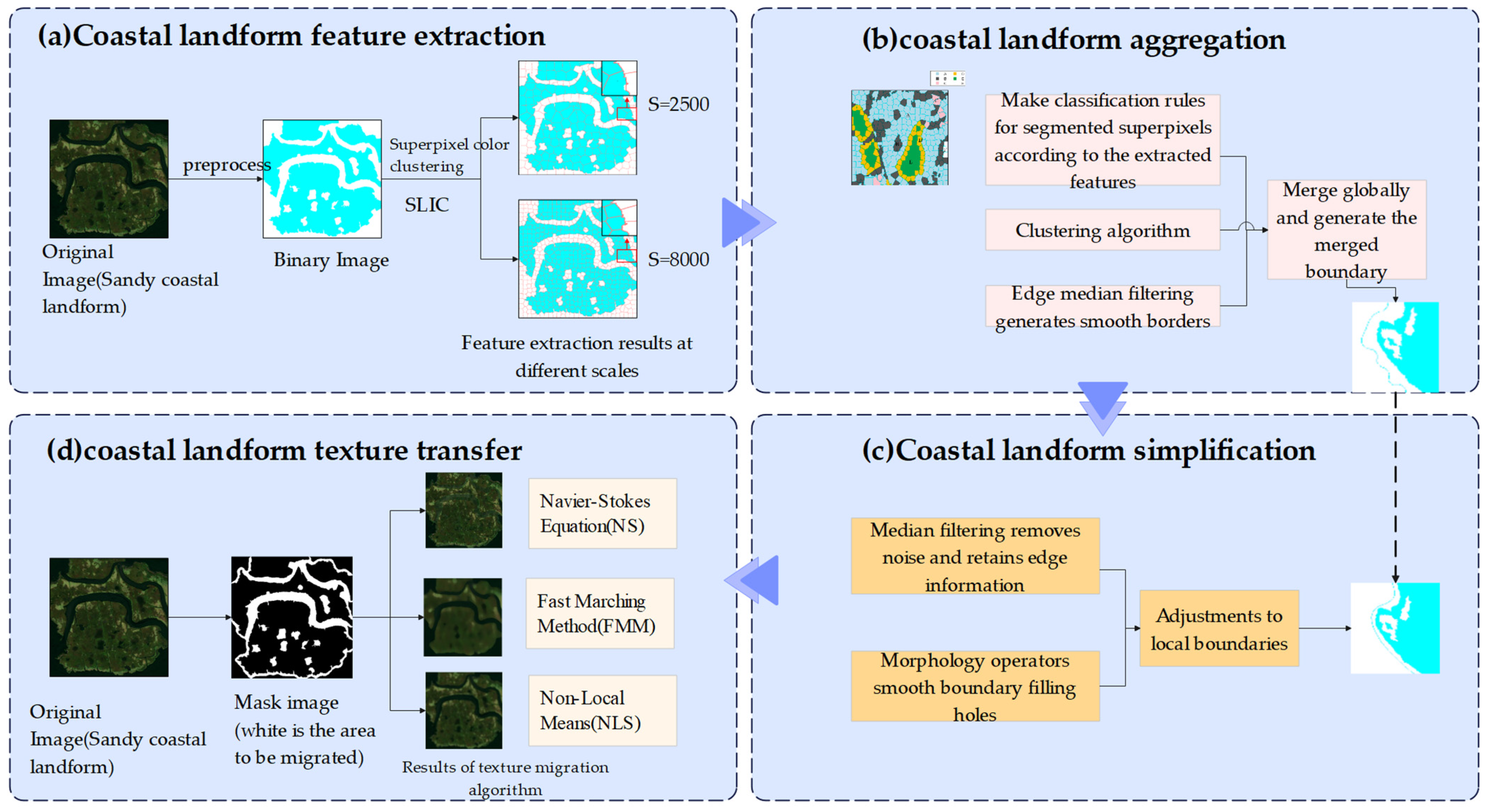
Figure 1. METF-C overall technical framework. (a) Coastal landform feature extraction; (b) Coastal landform aggregation; (c) Coastal landform simplification; (d) Coastal landform texture transfer.
Remotesensing 16 03862 g001
Figure 2. SLIC segmentation of coastal landform. (a) Original remote sensing images of marine coastal landform. The first is the marine coastal landform, and the second is the sandy coastal landform; (b) binary image preprocessed from the original image; (c) superpixel segmentation results at the level of 800 superpixels; (d) superpixel segmentation results at the level of 250 superpixels. Red ovals represent local boundary detail comparison of the sandy landform image at S = 800 and S = 250, and black ovals represent the local boundary detail comparison of the first marine sediment landform image at S = 800 and S = 250.
Remotesensing 16 03862 g002
Figure 3. Flowchart of the SLIC algorithm.
Remotesensing 16 03862 g003
Figure 4. Results of coastal landform superpixel simplification. Sample Image 1 and Sample Image 2 are two different data in the same coastal landform. Scale I represents the superpixel simplification results of different example maps at the level of superpixel number S = 2000. Scale II represents the superpixel simplification results of different example maps at the level of superpixel number S = 8000. The red boxes represent the smoothness of the boundaries at different levels, which is how the boundary features change.
Remotesensing 16 03862 g004
Figure 5. Median filtering smoothing adjustment of the merged boundary. (a) Result of the global simplified boundary under multi-scale I: that is, the number of superpixels is 2000 and the filtering core is 11. (b) Result of the global simplified boundary under the same Scale I and the filtering core is 45. (c) Result of the global simplified boundary under multi-scale Scale II: that is, the number of superpixels is 8000 and the filtering core is 11. (d) Result of the global simplified boundary under the same Scale II and filtering core is 45, mainly to analyze the influence of the hierarchy and filtering check on the global simplified result.
Remotesensing 16 03862 g005
Figure 6. Texture transfer process. (a) Black and white binary image. (b) The filled graph of the generated boundary.
Remotesensing 16 03862 g006
Figure 7. Sandy coastal and marine sediment coastal landform data. The red square indicates our study area which near New York.
Remotesensing 16 03862 g007
Figure 8. Coastal geomorphic feature extraction by SLIC. Sample Images 1 and 2 represent sandy coast landform images, and Sample Images 3 and 4 represent marine sediment coast landform images. (a1a4) represent the original remote sensing satellite images of the four coastal landforms. (b1b4) represent the coastal landform images that are preprocessed into binary images. (c1c4) represent the segmentation and clustering of the four sample maps at the scale of 250 superpixels. (d1d4) represent the segmentation and clustering of four sample graphs on the scale of 800 superpixels, where the corresponding arrow in square brackets indicates the enlarged map of the boundary, which is convenient for feature extraction and analysis of the boundary.
Remotesensing 16 03862 g008
Figure 9. Comparison of the merging effect of the METF-C method and the ArcGIS method in detail (Level II). (a1a4) Merging results of the METF-C method. (b1b4) Merging results of the ArcGIS method. Below the merging result is the enlarged image of the red box area. The blue line is the boundary between the two methods.
Remotesensing 16 03862 g009
Figure 10. Results of METF-C texture transfer experiment. (a1,b1,c1,d1) sample images; (a2,b2,c2,d2) mask images for the transfer; (a3,b3,c3,d3) METF-C texture transfer results.
Remotesensing 16 03862 g010
Figure 11. Comparison of experimental results between median filtering, image pyramid, Gaussian filtering, and METF-C method. The dashed ovals in different colors indicate our study areas with different methods.
Remotesensing 16 03862 g011
Table 1. Comparison of different texture transfer methods.
MethodMSEPSNRNMISSIM
NS17.98935.5810.2580.961
FMM19.65035.1970.2610.910
NL-Means28.67633.5560.2550.816
Table 2. Aggregation parameter settings for METF-C and ArcGIS.
LevelMethodNumber of the Superpixels (S)Radius of Filtering Kernel (R)Aggregation Distance
IMETF-C250045-
ArcGIS--100 m
IIMETF-C12,50011-
ArcGIS--150 m
Table 3. Parameter settings corresponding to the METF-C method, median filtering, image pyramid, and Gaussian filtering at two levels. Kernel size represents the size of the median filtering kernel and the Gaussian kernel; scale factor represents the ratio of each layer of images in the image pyramid to the previous layer of images; sigma controls the width of the Gaussian kernel; ‘-’ indicates that the value is empty.
LevelMethodNumber of Superpixels (S)Kernel SizeScale FactorSigma
IMETF-C250045--
Median filtering-5--
Image pyramid--2-
Gaussian filtering-3-1
IIMETF-C12,50011--
Median filtering-7--
Image pyramid--4-
Gaussian filtering-5-2
Table 4. Comparison of Edge Preservation Index (EPI), Texture Clarity Score (TCS), and Information Retention Rate (IRR) for METF-C, median filtering, image pyramid, and Gaussian filtering under two different scales (Scale I and Scale II).
LevelMethodEdge Preservation IndexTexture Clarity ScoreInformation Retention Rate
IMETF-C0.98839.0862.175
Median filtering0.9780.5421.947
Image pyramid0.86145.1072.084
Gaussian filtering0.935.922.104
IIMETF-C0.9831.3872.087
Median filtering0.9671.0922.330
Image pyramid0.9821.4312.027
Gaussian filtering0.921.522.075
Disclaimer/Publisher’s Note: The statements, opinions and data contained in all publications are solely those of the individual author(s) and contributor(s) and not of MDPI and/or the editor(s). MDPI and/or the editor(s) disclaim responsibility for any injury to people or property resulting from any ideas, methods, instructions or products referred to in the content.