Abstract
Microwave coincidence imaging (MCI) represents a novel forward-looking radar imaging method with high-resolution capabilities. Most MCI methods rely on random frequency modulation to generate stochastic radiation fields, which introduces the complexity of radar systems and imposes limitations on imaging quality under noisy conditions. In this paper, microwave coincidence imaging with phase-coded stochastic radiation fields is proposed, which generates spatio-temporally uncorrelated stochastic radiation fields with phase coding. Firstly, the radiation field characteristics are analyzed, and the coding sequences are designed. Then, pulse compression is applied to achieve a one-dimensional range image. Furthermore, an azimuthal imaging model is built, and a reference matrix is derived from the frequency domain. Finally, sparse Bayesian learning (SBL) and alternating direction method of multipliers (ADMM)-based total variation are implemented to reconstruct targets. The methods have better imaging performance at low signal-to-noise ratios (SNRs), as shown by the imaging results and mean square error (MSE) curves. In addition, compared with the SBL and ADMM-based total variation methods based on the direct frequency-domain solution, the proposed method’s computational complexity is reduced, giving it great potential in forward-looking high-resolution scenarios, such as autonomous obstacle avoidance with vehicle-mounted radar and terminal guidance.
1. Introduction
Synthetic aperture radar (SAR) and inverse synthetic aperture radar (ISAR) are two main techniques used for high-resolution radar imaging. The two methods rely on the relative motion between the radar and targets to form a virtual aperture [1,2,3]. However, in the forward-looking region, the viewing angle of the radar remains nearly unchanged, thus making it difficult to form a large virtual aperture, which limits the imaging performance [4,5].
Microwave coincidence imaging (MCI) is a forward-looking imaging method with high azimuthal resolution [6,7,8]. It generates stochastic radiation fields in the imaging region by modulating transmitted signals [9,10,11]. The targets can be distinguished by the stochastic radiation fields. Then, they can be reconstructed by correlating echo signals with reference signals. In contrast to other forward-looking radar imaging methods [12,13,14,15], microwave coincidence imaging no longer relies on the relative motion between the radar and targets, breaking the azimuthal resolution limitations of a real aperture.
MCI in the literature mainly adopts random frequency modulation. Different array elements transmit random frequency signals to generate spatio-temporally uncorrelated stochastic radiation fields [16,17,18]. However, this method increases the system complexity. Furthermore, the presence of different frequency signals at the same moment makes it difficult to perform pulse compression on echo signals, which means that the imaging distance is limited and the quality is sensitive to noise.
Sparse recovery [19,20,21] and compressed sensing (CS) [22,23,24] can be applied in microwave coincidence forward-looking imaging; these methods have high imaging resolution for simple targets composed of strong scattering points, such as angular antipodal, metal balls, etc. However, for complex-structure targets, such as aircraft and tanks, the imaging reconstruction capability is inadequate, making it challenging to reconstruct the contours and target structural features accurately.
In this paper, a microwave coincidence imaging method based on phase modulation is proposed. This method can utilize a phased array system to generate spatio-temporally uncorrelated stochastic radiation fields. Wavefront entropy and effective rank are selected to analyze the radiation field characteristics, which are used to guide the design of the phase encoding. Then, a one-dimensional range image in the frequency domain is obtained by applying pulse compression to the echo signal. At this point, the range dimension has been segregated from the azimuthal dimension. Consequently, an azimuthal dimensional imaging equation in the frequency domain can be established, and a reference matrix in the azimuthal dimension can be derived. The reconstruction of the target is achieved by stitching together azimuthal scattering coefficients at different distances, which reduces the computational complexity. Finally, the imaging equations are solved by using sparse Bayesian learning (SBL) and alternating direction method of multipliers (ADMM)-based total variation methods. The results of the simulations demonstrate that the method proposed in this paper can achieve better imaging performance at low signal-to-noise ratios (SNRs) [25] with lower complexity.
2. Radiation Field Generation
The characteristics of the stochastic radiation field determine the imaging quality. The traditional radiation field generated by random modulation has better random characteristics, but it poses problems, such as great difficulty in solving imaging equations and poor imaging robustness. Thus, a stochastic radiation field generation method based on phase modulation is proposed, and the phase code of the transmitted signals is designed in this paper.
2.1. Radiation Field Characterization
Radar systems transmit phase-coded linear frequency modulation signals through multiple antennas. Transmitted signals are superimposed on the target area to form a spatio-temporally uncorrelated radiation field, which is the basis of imaging. Assuming that the target is located in the region of the radiation field, an XOY coordinate system is established at the center of the target, as illustrated in Figure 1.
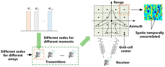
Figure 1.
Principle of radar coincidence imaging.
The radar system comprises N transmitting antennas and one receiving antenna. The imaging plane is assumed to be divided into L grids. A total of M modulations are performed. Each antenna transmits a distinct coded signal at different moments. At the mth modulation, the signal transmitted by the nth transmitter can be expressed as
where is the pulse width, A is the amplitude of the signal, is the carrier frequency, k is the frequency modulation coefficient, and is the phase of the nth array element at the mth modulation is fast time.
A cyclic code means that when any code element in a code group is shifted left or right by any number of bits, the resulting code element still belongs to the code group. The structural characteristics of the cyclic matrix have the advantage of reducing computational complexity [26], as some fast algorithms can be employed to solve the equations. Furthermore, the relatively high rank of the cyclic matrix renders it suitable for generating the radiation field [27,28].
When a cyclic code is used to encode the transmitted signals of N array elements, the coding matrix following M modulations can be expressed as
where each row represents the encoding of a different array element under one modulation, each column represents the encoding of an array element under a different number of modulations, and each row of this encoding matrix is shifted in the order of the previous row.
The design of the coding matrix is primarily concerned with the coding sequence of the first row [29]. Note that the sequence code in the first column is . is designed as a random code in the following analysis of radiation field characteristics.
The radar system transmits the signals defined in (1), and the scattering point is an ideal scattering point with a scattering coefficient of 1. The reference signals can be expressed as a superposition of the received signals in each grid. When the radar system undergoes M modulations, the expression of the reference signals is as follows:
where , is the position vector of the lth grid, is the position vector of the nth transmitting antenna, is the position vector of the receiving antenna, and c is the propagation speed of electromagnetic waves.
When satisfies , the reference signals’ matrix form can be written as
where denotes the number of samples.
Assuming that the target scattering coefficient of each divided grid cell is , the echo of the superimposed reference signals at the mth modulation is given by
In order to analyze the characteristics of the radiation field, it is first necessary to define the radiation field evaluation metric. Since the wavefront modulation changes the randomness of the radiation field by changing the undulation of the wavefront, the wavefront entropy is defined. It represents the magnitude of wavefront undulation using the statistical average of the radiation field amplitude over a period of time. Its expression is as follows [30]:
where is the signal reference matrix, L denotes the number of grids, and Q denotes the number of modulations. is the probability of the statistical distribution of elements in the qth row of S, .
The second evaluation metric is the effective rank [31]. The S singular value decomposition can be expressed as follows:
The effective rank is typically determined through the Frobenius paradigm ratio, where the previous matrix is approximated by a large singular value matrix whose singular value is the original matrix decomposition. This approximated matrix is then compared to the Frobenius paradigm ratio to S.
The largest value of r satisfying is taken as the effective rank of the matrix S, where ε is a value close to 1.
The following section will analyze the variation characteristics of evaluation metrics for different bandwidths, array spacing, and number of codes.
The transmitting array is a 16 × 1 linear array with a spacing of 0.15 m. is 90 GHz; the bandwidths are 200 MHz, 400 MHz, 600 MHz, and 800 MHz; the pulse width is 200 ns; and the imaging plane is divided into a grid of 30 × 30 with a size of 0.5 m × 0.5 m.
Figure 2 illustrates the undulations of the radiation field at the same moment at varying bandwidths, and Table 1 is the statistical average of wavefront entropy. It can be observed that as the bandwidth increases, the undulations of the radiation field become increasingly sharp at this moment, and the value of wavefront entropy also increases gradually. The value of wavefront entropy demonstrates that the randomness of the radiation field can be increased by expanding the bandwidth.
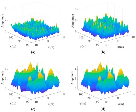
Figure 2.
Wavefront undulations of different bandwidths at the same moment. (a) B = 200 MHz. (b) B = 400 MHz. (c) B = 600 MHz. (d) B = 800 MHz.

Table 1.
Value of wavefront entropy.
Figure 3a depicts the trend of the effective rank for varying bandwidths. The number of sampling points is 400. Other parameters are consistent with the preceding analysis. It can be observed that the effective rank increases as the bandwidth increases.
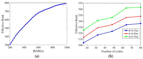
Figure 3.
Effective-rank change curves for different influencing factors. (a) Effective-rank change curves at different bandwidths. (b) Effective-rank change curves with different array spacings and numbers of codes.
In order to analyze the influence of the array element spacing and the number of codes on the effective rank, a simulation was conducted using different array element spacings and numbers of codes. The results are presented in Figure 3b. It can be seen that increasing either the array element spacing or the number of codes can effectively increase the effective rank and increase the randomness of the radiation field.
2.2. Design of Code Sequence
While produces radiation fields with high randomness when it is randomly coded, this introduces uncertainty. The effective rank of the reference matrix will change with each image acquisition, and its size fluctuates widely. When the effective rank is large, the imaging quality is high, while when the effective rank is small, the imaging quality is poor. This uncertainty introduces variations that are challenging to grasp, resulting in an imaging quality that is not robust.
Chaotic sequences exhibit both intrinsic determinism and extrinsic randomness. For a given mapping, the generated code elements are deterministic, while the generated code elements exhibit random properties among themselves. Therefore, is considered to be encoded as a chaotic sequence, and the logistic mapping is selected to generate the chaotic sequence. The mapping equation is as follows:
where µ is a system parameter, [32], and .
When , the logistic mapping enters a chaotic state, producing chaotic sequences with high randomness.
In order to enhance the randomness of the chaotic sequences generated by the logistic mapping, the generated sequence will be converted using the inverse sine function [33].
The system parameter values are designated as and initial value . The 20th chaotic sequence is designated as the starting value, and every 10th sequence value is extracted as the desired code, resulting in a total of 16 codes for .
Figure 4 illustrates the undulations of the radiation field when is a chaotic sequence generated by logistic mapping. It can be observed that a radiation field with considerable undulations can still be generated, with a wavefront entropy of 3.1214 and an effective rank of 752.
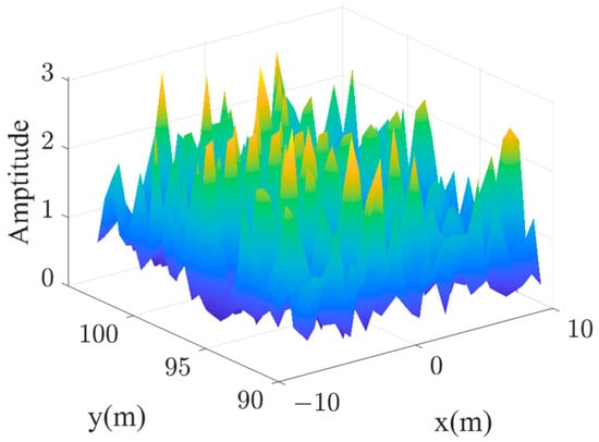
Figure 4.
Radiation field distribution of chaotic sequences generating cyclic codes.
Figure 5 illustrates the variation in effective rank when is a chaotic sequence and a random code for different imaging times at different bandwidths. The value of effective rank when is coded as a chaotic sequence is comparable to the high effective rank when is coded as a random code. And, it exhibits extrinsic deterministic properties that contribute to robust imaging when is a chaotic sequence.
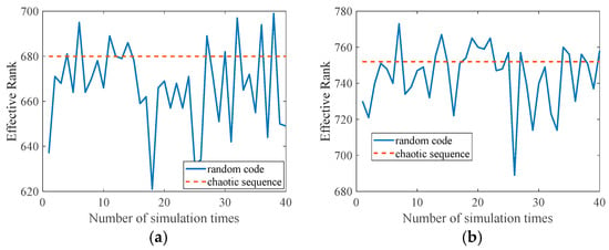
Figure 5.
Variation in the effective rank corresponding to random codes and chaotic sequences for different imaging times. (a) B = 600 MHz. (b) B = 800 MHz.
3. Imaging Model
Wavefront-modulated forward-looking imaging with phase coding offers two significant advantages. Firstly, unlike frequency modulation, the echo signals with phase modulation have the same frequency and differ only in phase. This enables echoes to be processed by pulse compression, which can improve imaging performance at low SNRs. Secondly, phase coding employs a coding sequence that is both deterministic and random, thereby increasing the robustness of the imaging process.
For transmitted signals with phase coding, as illustrated in (1), the echo signals obtained by the superposition of all array elements under M modulations can be expressed as follows:
where is the scattering coefficient in the lth grid.
The echo signals have the same frequency at the same time, and only a phase difference exists. Therefore, the dechirping method can be used for echoes. The reference signal for dechirping is defined as
The differential frequency output is obtained by multiplying the echo signals conjugated to the reference signal:
The one-dimensional range image of the target in the frequency domain is obtained by Fourier transformation. The different frequency points thus correspond to different distances:
At this point, the range dimension of the target has been segregated from the azimuthal dimension. The same operation described above is performed on the reference matrix to obtain its representation in the frequency domain:
The frequency-domain reference signal matrix form can be expressed as
where denotes the number of samples in a pulse.
In order to reduce the computational complexity, the azimuthal scattering coefficients of targets are reconstructed at different distances separately. Subsequently, the scattering coefficients of all distances are spliced together to obtain the complete scattering coefficients of the target.
Assuming that is the peak frequency of the one-dimensional range image obtained by pulse compression, the frequency-domain echoes at a distance corresponding to the frequency can be expressed as follows:
Then, the reference signals at a distance corresponding to can be expressed as
where , , denotes the distance delay, denotes the delay of the azimuthal grid at this distance, is the azimuthal position vectors of the lth grids, and is the range position vectors of the lth grids.
The reference matrix grid is a patchwork of azimuthal grids at different distances when computed directly, but when solving from the azimuthal dimension, the number of grids in the reference matrix becomes the number of azimuthal grids at one distance. A new reference matrix is formed by taking out the reference signals at that distance under each modulation. Its form at a single distance can be expressed as follows:
where represents the number of azimuthal grids. Each row denotes the reference signals in different azimuthal grids for a single pulse, while each column denotes the reference signals for different pulses in a single azimuthal grid.
Thus, when modulated M times, the imaging equation at a single distance can be expressed as
where n is Gaussian white noise.
The azimuthal target scattering coefficients are obtained by solving (20). Target reconstruction can be achieved by traversing each distance and stitching the azimuthal target scattering coefficients from each solution.
4. Imaging Algorithm and Results
4.1. Sparse Bayesian Learning
SBL [34] first assumes that the target scattering coefficient distribution satisfies the prior. The reconstructed target is then achieved by solving the maximum a posteriori estimate in the Bayesian framework using prior information. At this point, the question form becomes
The problem can be transformed by the Bayesian formulation:
Assume that the noise follows a Gaussian distribution, where the mean is 0 and the variance is .
Assume that is generated by the hyperparameter
where , and .
Considering the exponential part as a whole, the derivation and collation of the calculations leads to
Further calculations based on (22) give the mean and variance of the scattering coefficient:
The hyperparameters are updated by the EM algorithm:
In order to verify the effectiveness of the phase modulation azimuthal dimensional imaging model (AziPM) proposed in this paper, a sparse Bayesian learning imaging algorithm was used to image a point aircraft target, as shown in Figure 6. The imaging results of the traditional frequency modulation (FM) method are compared, and the simulation parameters are shown in Table 2.
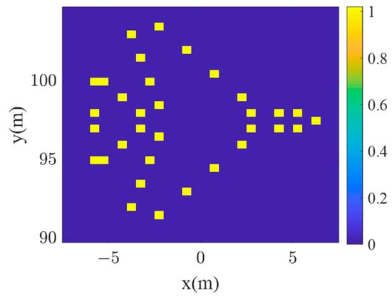
Figure 6.
Aircraft point targets.

Table 2.
Simulation parameters.
Figure 7 illustrates that the AziPM method achieves satisfactory reconstruction results at both 0 dB and 5 dB, with superior imaging results compared to the FM method.
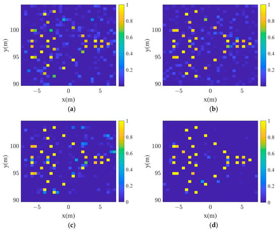
Figure 7.
SBL imaging results. (a) FM results at 0 dB. (b) FM results at 5 dB. (c) AziPM results at 0 dB. (d) AziPM results at 5 dB.
Figure 8 plots the azimuthal dimensional slices in the second row of target distances for both methods at 0 dB. It can be seen that the azimuthal slices of the proposed method possess lower sidelobes compared to those of the FM method, which further indicates that the method is able to obtain better imaging performance.
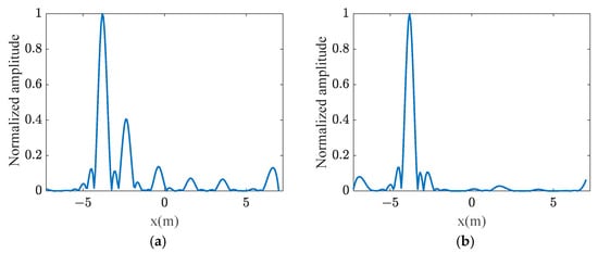
Figure 8.
Azimuthal dimensional slices at 0 dB. (a) FM method. (b) AziPM method.
In order to quantitatively analyze the quality of imaging, the mean square error (MSE) is defined by the following expression:
Figure 9a depicts the MSE-versus-SNR curves of the two methods. It can be observed that the MSE curve of the AziPM method is considerably lower than that of the FM method, which suggests that the imaging performance of the AziPM is superior to that of the FM method.
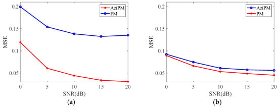
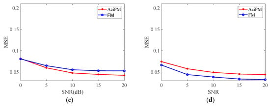
Figure 9.
MSE curves of FM and AziPM methods with different modulation counts: (a) 16 modulations, (b) 48 modulations, (c) 64 modulations, (d) 96 modulations.
Figure 9 shows the comparison of the MSE curves of the two methods for different numbers of modulations.
It can be observed that the MSE of the AziPM method is considerably lower than that of the FM method when the number of modulations is limited. As the number of modulations gradually increases, the relative MSE curves of the two methods gradually converge, and the final performance of the conventional FM method approaches that of the AziPM method. The final results demonstrate that while the FM method can generate a radiated field with a higher degree of stochasticity, this must be achieved when the number of modulations is sufficiently large. Conversely, the AziPM method is capable of achieving a lower MSE with a smaller number of modulations.
In order to compare the effects of circular coding and random coding on the imaging performance, Figure 10 shows the results of imaging simulations carried out at 0 dB for both codes. As can be seen from the results, there is little difference between the two coded imaging effects. In order to analyze the effects qualitatively, Figure 11 plot the MSE curves at different SNR. It can be seen that, although the reference matrix rank generated by the cyclic code is not as high as that obtained with the random code, the cyclic code MSE is lower than the random code MSE after Monte Carlo due to its robustness.
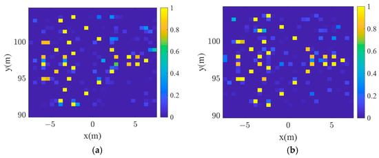
Figure 10.
Imaging results with different codes at 0 dB. (a) Cyclic code. (b) Random code.
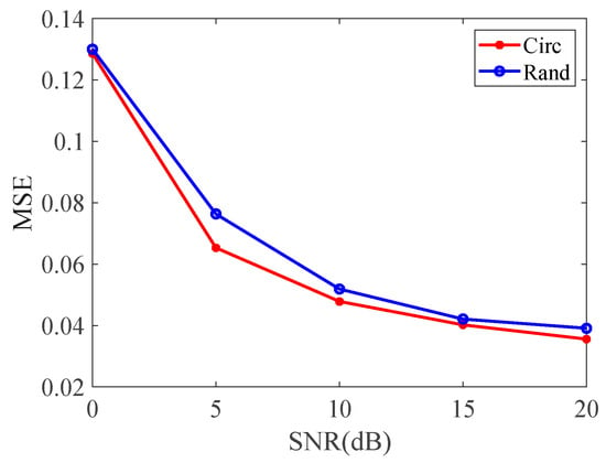
Figure 11.
MSE curves of cyclic code and random code methods.
The AziPM method for target reconstruction is effective when the scattering points in the azimuthal direction are sparsely distributed, allowing for effective reconstruction at a low SNR. However, when the number of azimuthal scattering points increases and the complexity of the target increases, the imaging results are gradually drowned in noise. It is already difficult to perform a complete reconstruction of the target using the SBL method. Figure 12 illustrates the imaging results of three targets at 0 dB and 5 dB. It is evident that as the complexity of the target increases, the SBL method is unable to reconstruct the target effectively.
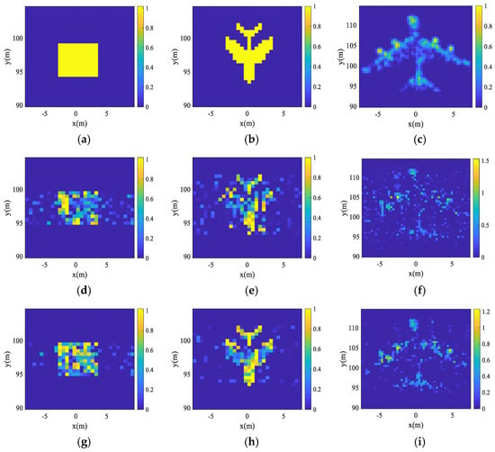
Figure 12.
Imaging results for different targets. (a–c) Targets. (d–f) Imaging results at 0 dB. (g–i) Imaging results at 5 dB.
4.2. ADMM-Based Total Variation
The total variation regularization method was initially employed in the field of image processing [35], where the total variation model permitted the solution to be discontinuous [36]. This enabled the retention of edge and contour information in the image while denoising.
The total variable is defined as follows:
where is the derivative of the reference coefficient in grid l, is the reference matrix, and is the echo vector. It is anisotropic total variation when and isotropic total variation when .
By employing the Lagrangian method to introduce convex relaxation, the objective function can be transformed into the following form:
Given that is not derivable within the paradigm term , a slack variable w is introduced to replace [37], resulting in the following model:
The objective function undergoes a transformation from the quadratic penalty function to
Consequently, the alternating iterative multiplier method can be employed to transform the original problem into the resolution of two subproblems, namely, the solution of w and that of , in consecutive iterations.
4.2.1. w Sub-Problem
When is determined, (35) becomes
When , it follows that
When , it follows that
4.2.2. Sub-Problem
When w is determined, (35) becomes
In each iteration, the value of needs to be updated in accordance with the following equation:
The solution to (39) can be obtained by means of the fastest descent method. The iterative solution equation is as follows:
where is the derivative of (29) and can be expressed as
The most rapid single-step descent can be applied to
where k denotes the number of iterations, and denotes the step size.
According to the literature [38], can be determined by the following equation:
where , and .
The initial value of can be derived from the following equation:
The following conditions need to be satisfied between two iterations:
where is defined as follows:
In the simulation, was selected.
With the above iterations, can be solved.
The same three targets were reconstructed by using the ADMM-based total variation method. The resulting imaging results are presented in Figure 13.
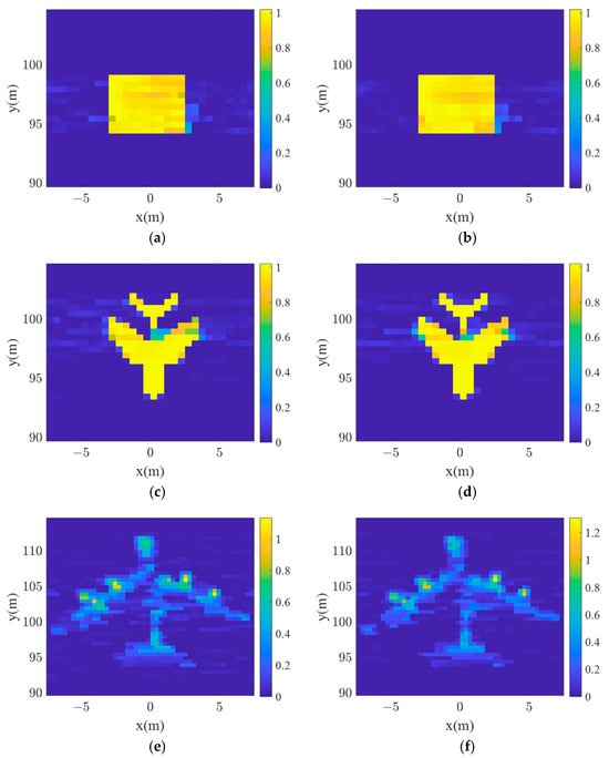
Figure 13.
ADMM total variation imaging results. (a,c,e) Imaging results at 0 dB. (b,d,f) Imaging results at 5 dB.
Comparing SBL with the ADMM-based total variation method reveals that the latter has the capacity to reconstruct the structure of the target more completely and to perform better edge reconstruction.
In order to quantitatively analyze the effect of the ADMM-based total variation method on the imaging quality, the MSE curves of this method and the other four methods at different SNRs are plotted in Figure 14. This figure shows that the MSE curves of the five methods all demonstrate a decreasing trend as the SNR increases. The MSEs of the AziPM and PM methods are roughly the same when imaging, whether using the SBL or ADMM-based total variation algorithm. The MSE of FM-SBL is relatively high, while AziPM-TV has the lowest MSE among the different methods, with the curve located at the bottom. This further indicates the effectiveness of the method proposed in this paper.
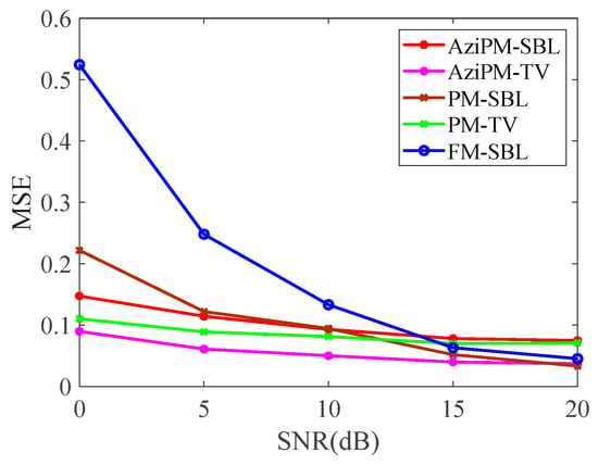
Figure 14.
MSE curves for different methods.
Figure 15 compares the runtimes of the four methods, demonstrating that the total variation method yields a more accurate solution with a longer runtime. However, by solving the azimuthal dimensions at each distance sequentially, the computational complexity can be greatly reduced. The runtime can be reduced by about 3.8 compared with solving directly with the SBL algorithm and can be reduced by about 5.5 compared with solving directly with ADMM-based total variation.
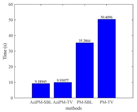
Figure 15.
Comparison of runtimes of different methods.
5. Conclusions
In this paper, microwave coincidence imaging with phase-coded stochastic radiation fields is proposed. Firstly, due to the characteristics of phase modulation, the pulse compression technique is utilized in the microwave coincidence imaging process to obtain a one-dimensional range image in the frequency domain. Then, the equation in the azimuthal dimension is established, and the reconstruction of the target can be achieved by correlating echo signals with reference signals at different distances in the frequency domain. SBL and ADMM-based total variation methods were used to reconstruct targets. The two algorithms achieved good imaging results at low SNRs, but ADMM-based total variation could achieve better reconstruction of the edge structure of complex targets. The runtime of the proposed method can be reduced compared with the direct frequency-domain solution. The method can be applied to forward-looking radar imaging scenarios, such as autonomous obstacle avoidance with vehicle-mounted radar and terminal guidance.
Author Contributions
Writing—original draft preparation, H.L. (Hang Lin); writing—review and editing, H.L. (Hang Lin), H.L. (Hongyan Liu), Y.C., K.X., K.L. and Y.Y.; supervision, H.L. (Hongyan Liu); conceptualization and methodology, H.L. (Hang Lin); investigation, H.L. (Hongyan Liu). All authors have read and agreed to the published version of the manuscript.
Funding
This work was supported in part by the National Key Research and Development Program of China under Grant 2022YFB3902400, in part by the Distinguished Youth Science Foundation of Hunan Province under Grant 2022JJ10063, and in part by the National Natural Science Foundation of China under Grant 62322122.
Data Availability Statement
The original contributions presented in the study are included in the article, further inquiries can be directed to the corresponding author.
Conflicts of Interest
The authors declare no conflicts of interest.
References
- Sun, M.; Qi, F.; Zhao, Y.; Ji, C. Resolution enhancement based on antenna aperture compensation in synthetic aperture radar imaging with hyper-laplacian prior deconvolution. IEEE Sens. J. 2019, 23, 21679–21686. [Google Scholar] [CrossRef]
- Wu, H.; Cheng, Y.; Chen, X. Information geometry-based track-before-detect algorithm for slow-moving fluctuating target detection. IEEE Trans. Signal Process. 2023, 71, 1833–1848. [Google Scholar] [CrossRef]
- Wu, H.; Cheng, Y.; Chen, X. Power spectrum information geometry-based radar target detection in heterogeneous clutter. IEEE Trans. Geosci. Remote Sens. 2024, 62, 5102016. [Google Scholar] [CrossRef]
- Wu, J.; Li, Z.; Huang, Y. Focusing bistatic forward-looking SAR with stationary transmitter based on keystone transform and nonlinear chirp scaling. IEEE Geosci. Remote Sens. Lett. 2014, 11, 148–152. [Google Scholar] [CrossRef]
- Yang, J. Multi-directional evolution trend and law analysis of radar ground imaging technology. J. Radars. 2019, 8, 669–692. [Google Scholar]
- Li, D.; Li, X.; Qin, Y. Radar coincidence imaging: An instantaneous imaging technique with stochastic signals. IEEE Trans. Geosci. Remote Sens. 2014, 52, 2261–2277. [Google Scholar]
- Zhu, S.; Zhang, A.; Xu, Z. Radar coincidence imaging with random microwave source. IEEE Antennas Wirel. Propag. Lett. 2015, 14, 1239–1242. [Google Scholar] [CrossRef]
- Guo, Y.; He, X.; Wang, D. A novel super-resolution imaging method based on stochastic radiation radar array. Meas. Sci. Technol. 2013, 24, 074013. [Google Scholar] [CrossRef]
- He, X.; Liu, C.; Liu, B. Sparse frequency diverse MIMO radar imaging for off-grid target based on adaptive iterative MAP. Remote Sens. 2013, 5, 631–647. [Google Scholar] [CrossRef]
- Zhao, M. Frequency-diverse metacavity cassegrain antenna for differential coincidence imaging. IEEE Trans. Antennas Propag. 2023, 71, 9054–9059. [Google Scholar] [CrossRef]
- Cao, K.; Cheng, Y.; Liu, Q. Microwave coincidence imaging based on attributed scattering model. IEEE Signal Process. Lett. 2022, 29, 1694–1698. [Google Scholar] [CrossRef]
- Wu, J.; Sun, Z.; Yang, J. Star-machine dual-base SAR imaging based on GF-3 irradiation and experimental validation. Radar Sci. Technol. 2021, 19, 241–247. [Google Scholar]
- Zhang, Y. Fast inverse-scattering reconstruction for airborne high squint radar imagery based on doppler centroid compensation. IEEE Trans. Geosci. Remote Sens. 2022, 60, 5205517. [Google Scholar] [CrossRef]
- Zhu, Y.; He, M.; He, Z. Joint minimum variance and maximum likelihood spectral estimation for forward-looking imaging methods. Syst. Eng. Electron. 2023, 45, 3108–3115. [Google Scholar]
- Li, W.; Zhang, B.; Li, K.; Yan, J. LRSD-ADMM-NET: Simultaneous super-resolution imaging and target detection for forward-looking scanning radar. Remote Sens. 2024, 17, 4052–4061. [Google Scholar] [CrossRef]
- Liu, Q.; Cheng, Y.; Cao, K. Radar 3-D forward-looking imaging for extended targets based on attribute scattering model. IEEE Geosci. Remote Sens. Lett. 2023, 20, 3502305. [Google Scholar] [CrossRef]
- Cao, K.; Cheng, Y.; Liu, K. Reweighted-dynamic-grid-based microwave coincidence imaging with grid mismatch. IEEE Trans. Geosci. Remote Sens. 2022, 60, 5102510. [Google Scholar] [CrossRef]
- Zhu, S.; He, Y.; Chen, X. Resolution Threshold Analysis of the Microwave Radar Coincidence Imaging. IEEE Trans. Geosci. Remote Sens. 2020, 58, 2232–2243. [Google Scholar] [CrossRef]
- Zhou, X.; Fan, B.; Wang, H. Sparse Bayesian perspective for radar coincidence imaging with array position error. IEEE Sens. J. 2017, 17, 5209–5219. [Google Scholar] [CrossRef]
- Tian, B.; Zhang, X.; Tang, X. A joint sparse recovery algorithm for coprime adjacent array synthetic aperture radar 3D sparse imaging. Int. J. Remote Sens. 2021, 42, 6560–6580. [Google Scholar] [CrossRef]
- Lu, X.; Yang, J.; Tan, K. Range-Doppler image reconstruction for collocated MIMO noise radar by sparse recovery. Remote Sens. Lett. 2022, 13, 279–289. [Google Scholar] [CrossRef]
- Candès, J.; Wakin, M. An introduction to compressive sampling: A sensing sampling paradigm that goes against the common knowledge in data acquisition. IEEE Signal Process. 2008, 25, 21–30. [Google Scholar] [CrossRef]
- Xu, G.; Zhang, B.; Yu, H.; Chen, J. Sparse Synthetic Aperture Radar Imaging from Compressed Sensing and Machine Learning: Theories, applications, and trends. IEEE Geosci. Remote Sens. 2022, 10, 32–69. [Google Scholar] [CrossRef]
- Seidi, M.; Shah, U.; Oberhammer, J. Analysis of a Minimalistic Imaging Radar Concept Employing Beam Shape Switching and Compressed Sensing. IEEE Trans. Geosci. Remote Sens. 2024, 62, 1–12. [Google Scholar] [CrossRef]
- Bai, X.; Wang, G.; Liu, S. High-Resolution Radar Imaging in Low SNR Environments Based on Expectation Propagation. IEEE Trans. Geosci. Remote Sens. 2021, 59, 1275–1284. [Google Scholar] [CrossRef]
- Hariprasad, M. Circulant decomposition of a matrix and the eigenvalues of Toeplitz type matrices. Appl. Math. Comput. 2024, 468, 128473. [Google Scholar] [CrossRef]
- Heng, Z.; Wang, X.; Li, X. Constructions of cyclic codes and extended primitive cyclic codes with their applications. Finite Fields Appl. 2023, 89, 102208. [Google Scholar] [CrossRef]
- Babur, G.; Aubry, P. Space-time radar waveforms: Circulating codes. Electr. Comput. Eng. 2013, 2013, 9. [Google Scholar] [CrossRef]
- Zhu, J.; Xie, Z.; Jiang, N. Delay-Doppler map shaping through oversampled complementary sets for high speed target detection. Remote Sens. 2024, 16, 2898. [Google Scholar] [CrossRef]
- Zou, L. Study of wavelet entropy for airport pavement inspection using a multistatic ground-penetrating radar system. Geophysics 2021, 86, 69–78. [Google Scholar] [CrossRef]
- Zhang, X. Singular value analysis. In Matrix Analysis and Application, 2nd ed.; Tsinghua Univ. Press: Beijing, China, 2013; pp. 301–312. [Google Scholar]
- Mankar, V.; Das, T.; Sarkar, S. Discrete chaotic sequence based on logistic map in digital communications. arXiv 2012, arXiv:1207.2694. [Google Scholar]
- Li, C.; Li, Y. Research on statistical characteristics of chaotic pseudorandom sequence for one-dimensional Logistic map. Appl. Res. Comput. 2014, 5, 1403–1406. [Google Scholar]
- Fan, B.; Zhou, X.; Chen, S. Sparse bayesian perspective for radar coincidence imaging with model errors. Math. Probl. Eng. 2020, 2020, 9202654. [Google Scholar] [CrossRef]
- Xiao, Y.; Yang, J. A fast algorithm for total variation image reconstruction from random projections. Mathematics 2010, 6, 547–563. [Google Scholar]
- Wang, Y. A new alternating minimization Algorithm for total variation image reconstruction. Imaging Sci. 2008, 1, 248–272. [Google Scholar] [CrossRef]
- Liu, X. Augmented lagrangian method for total generalized variation based poissonian image restoration. Comput. Math. Appl. 2013, 71, 1649–1705. [Google Scholar] [CrossRef]
- Eltiyeb, A.; Salem, M. Adaptive hybrid mixed two-point step size gradient algorithm for solving non-linear systems. Mathematics 2023, 11, 2102. [Google Scholar] [CrossRef]
Disclaimer/Publisher’s Note: The statements, opinions and data contained in all publications are solely those of the individual author(s) and contributor(s) and not of MDPI and/or the editor(s). MDPI and/or the editor(s) disclaim responsibility for any injury to people or property resulting from any ideas, methods, instructions or products referred to in the content. |
© 2024 by the authors. Licensee MDPI, Basel, Switzerland. This article is an open access article distributed under the terms and conditions of the Creative Commons Attribution (CC BY) license (https://creativecommons.org/licenses/by/4.0/).