Article

Early Detection of Dendroctonus valens Infestation with UAV-Based Thermal and Hyperspectral Images

1
Key Laboratory for Forest Pest Control, College for Forestry, Beijing Forestry University, Beijing 100083, China
2
Institute of Forest Resource Information Techniques, Beijing 100091, China
*
Author to whom correspondence should be addressed.
Remote Sens. 2024, 16(20), 3840; https://doi.org/10.3390/rs16203840
Submission received: 16 August 2024 / Revised: 10 October 2024 / Accepted: 14 October 2024 / Published: 16 October 2024
(This article belongs to the Special Issue Application of Remote Sensing in Agroforestry (Third Edition))

Abstract

:
Dendroctonus valens is one of the main invasive pests in China, causing serious economic and ecological damage. Early detection and control of D. valens can help prevent further outbreaks. Based on unmanned aerial vehicle (UAV) thermal infrared and hyperspectral data, we compared the spectral characteristics of Pinus sylvestris var. mongolica in three states (healthy, early-infested, and dead), and constructed a classification model based on the random forest algorithm using four spectral datasets (reflectance, first derivative, second derivative, and spectral vegetation index) and one temperature parameter dataset. Our results indicated that the spectral differences between healthy and early-infested trees mainly occur in the near-infrared region, with dead trees showing different characteristics. While it was effective to distinguish healthy from early-infested trees using spectral data alone, the addition of a temperature parameter further improved classification accuracy across all datasets. The combination of the spectral vegetation index and temperature parameter achieved the highest accuracy at 93.75%, which is 3.13% higher than using the spectral vegetation index alone. This combination also significantly improved early detection precision by 13.89%. Our findings demonstrated the applicability of UAV-based thermal infrared and combined hyperspectral datasets in monitoring D. valens early-infested trees, providing important technical support for the scientific prevention and control of D. valens.

1. Introduction

The red turpentine beetle (RTB; Dendroctonus valens LeConte), belonging to the family Scolytidae and genus Dendroctonus, is a stem-boring insect originally from North and Central America [1]. It was first discovered in Shanxi Province, China, in 1998 and then rapidly spread to neighboring provinces, causing widespread mortality of pine trees. It continues to expand northwards. As a recent invasive pest in Northeast China, it was found in Chaoyang, Liaoning Province, and Chifeng, Inner Mongolia, bordering Chengde City, Hebei Province, in 2017. Subsequent detections in Fuxin, Huludao, Jinzhou, Liaoning Province, and Tongliao, Inner Mongolia Autonomous Region, indicate a continuing trend of spread, primarily affecting Pinus tabuliformis and Pinus sylvestris var. mongolica plantations, with an alarming potential to invade nature reserves [2]. A recent survey by Lu et al. [3] showed that from 2018 to 2022, the RTB was the second-largest forest invasive species in the Three-North Shelterbelt region, with an average affected area of 60,300 hectares annually. Suitability studies indicate that the RTB has a strong adaptability to different environments and a wide range of suitable habitats, posing an invasion risk to Jilin Province, Heilongjiang Province, and even the Greater Khingan Mountains forest region [4]. Therefore, effective control measures are essential.
In Northeast China, the RTB completes one generation per year. In late spring, adults begin to invade new host roots and lower stems, forming entry tunnels where sawdust and pine resin accumulate outside, creating a funnel-shaped mass that initially appears red and then weathers into grayish-white particles [5]. The mature larvae feed on the cambium and phloem at the tunnel’s end, blocking the vascular system and causing the tree to wilt and die [6]. The invasion holes, resin masses, and tunnels on the tree trunks are key indicators of RTB infestation. Additionally, the color of the host canopy changes after RTB infestation. Similar to the mountain pine beetle (MPB) and the spruce beetle (SBB) [7,8], the canopy color of the infected tree changes over time from green to yellow, then red, and finally gray (needleless). Scholars categorize these stages as green, red, and gray attack stages [9]. During the green attack stage, the needles of infected pine trees remain green, and the tree is alive with no visible symptoms. It has been found that the green stage represents an early-infested stage, where the density of the new RTB generation is highest at the base of the host tree trunk, whereas in the yellow and red canopy color stages, the RTB density is very low, as most RTBs have already left the tree [10]. The canopy discoloration in response to early infestation significantly lags, typically appearing in the second growing season, by which time most RTBs have completed their development and spread to other trees [11]. Thus, early detection of the RTB is crucial for identifying early-infested trees and taking measures to prevent further spread and outbreak. There is an urgent need for a rapid and effective method to monitor pine forests for the early-infested stage of RTBs.
Remote sensing technology is increasingly suitable for large-scale forest pest and disease monitoring applications by reducing spatial and temporal limitations. It has become a vital tool for monitoring pests and assessing plant health [12]. Landsat imagery is freely available, providing extensive historical data that allows for the acquisition of time-series information from several years ago. However, most studies focused on mapping tree mortality at high damage levels. The reduced spectral variability in large-scale, interconnected areas of red-attack trees enhances classification accuracy, as homogeneous regions are easier to classify and map [13]. Meddens et al. [14] found that Landsat images were unable to detect pixels within fewer than 40% of pines in the red stage with an acceptable accuracy. Regardless of whether operating at a single-tree or forest stand scale, higher resolution imagery is necessary to enhance classification accuracy in cases of low tree damage. WorldView-2 features very high spatial resolution (2 m) and spectral resolution (eight bands). Compared to Landsat, these factors are more conducive to mapping the health status of individual trees. Immitzer & Atzberger [15] successfully detected bark beetle infestation in Norway Spruce using eight-band WorldView-2 data, and the overall accuracy (OA) reached 76%. However, very high resolution satellite imagery is expensive, and image acquisition is affected by cloud cover and revisit time [16]. Although unmanned aerial vehicle (UAV) remote sensing systems have a smaller coverage area and are less suitable for large-scale monitoring, they offer several advantages. These include low operational costs, high mission flexibility, the ability to fly below cloud cover, and the capability to capture high-temporal and high-spatial resolution imagery. Additionally, UAVs can be equipped with various sensors, such as RGB cameras, multispectral cameras, hyperspectral cameras, and thermal imaging cameras [17]. For coniferous trees in the early-infested stage of stem-boring insect infestation, the needle color in the canopy does not show significant changes. Detecting these subtle variations typically requires sensors with high spatial, temporal, and spectral resolution. Hyperspectral remote sensing, characterized by narrow spectral bandwidths and the simultaneous expression of spatial and spectral information, can capture detailed spectral information that is difficult to observe with the naked eye, a capability beyond that of RGB and multispectral sensors [17,18]. Research has proven that hyperspectral imaging can differentiate the various stages of conifer damage caused by bark beetles. Ma et al. [19] used UAV-based hyperspectral imaging to classify Pinus yunnanensis trees infested by Tomicus yunnanensis. Lin et al. [20] successfully used hyperspectral imaging to differentiate the varying degrees of damaged trees affected by the pine shoot beetle (PSB). Gao et al. [21] used UAV-based hyperspectral images to demonstrate the potential of hyperspectral imaging for early monitoring of RTBs. Several studies have found that the near-infrared spectral curves of early-infested trees significantly decrease, indicating that the near-infrared region has the potential for early detection of beetle infestation [22,23,24]. Curran et al. [25] found that the scattering effect of needles can cause changes in near-infrared reflectance. Additionally, the closure of stomata to conserve water might also lead to a decrease in near-infrared reflectance [26]. Although hyperspectral imaging has the ability to distinguish subtle spectral changes, there are still challenges in accurately monitoring the early-infested stages of RTBs.
On the other hand, mature RTB larvae bore into the cambium and phloem at the ends of tunnels [5], blocking the vascular system [6]. This disrupts water transport tissues, leading to significant changes in needle moisture content of the early-infested trees. These studies indicate that changes in moisture content are also a critical indicator for monitoring stem-boring insects. The disturbance in moisture content affects temperature through leaf transpiration, causing slight changes in needle canopy temperature. This difference can be detected using thermal infrared (TIR) remote sensing [27]. Hais et al. [28] and Abdullah et al. [29] found that satellite thermal infrared data can be used to monitor forest stands affected by bark beetles. However, canopy surface temperature (CST) derived from satellite images is not suitable for precise analysis of small areas due to its coarser resolution compared to optical images. The advent of UAVs has facilitated the application of high-resolution thermal imaging with centimeter-level resolution from lightweight thermal cameras [30]. Calderón et al. [31] successfully used UAVs equipped with thermal cameras to monitor olive trees affected by Verticillium wilt (VW). Wang et al. [32] analyzed the feasibility of using UAV-based thermal infrared imaging to monitor Yunnan pine shoot beetle infestations in Pinus yunnanensis. They also demonstrated that changes in canopy temperature are related to stomatal conductance and transpiration. It is crucial for early detection of bark beetle infestations using thermal imaging. Therefore, this study aims to explore the potential of UAV-based thermal infrared imaging for early-infested stage monitoring of RTB infestations in P. sylvestris var. mongolica.
In recent years, several studies have used multi-source remote sensing data to extract canopy features and quantify forest pest damage [33]. However, no study has yet combined UAV-based TIR imaging data with hyperspectral data to monitor RTB infestation. We categorized P. sylvestris var. mongolica into three stages based on field survey: healthy, infested (refers to the early-infested stage of RTB infestation when the canopy is still green), and dead (red stage with canopy fully or mostly red). We extracted canopy reflectance and average canopy temperature from hyperspectral and thermal infrared images and calculated the first derivative, second derivative, vegetation indices, and temperature parameters. Additionally, we used the random forest algorithm to distinguish the different stages of trees. The main contributions of this study could be summarized as follows: (1) explore the potential of UAV-based thermal infrared in early monitoring of RTBs; (2) investigate the potential of UAV-based thermal infrared and hyperspectral combination data for monitoring the early-infested stage of RTBs at the individual tree level.

2. Materials and Methods

2.1. Study Area

The study area is located in the Heilihe National Nature Reserve in Ningcheng County, Chifeng City, Inner Mongolia Autonomous Region. The reserve is situated at the border between Inner Mongolia Autonomous Region and Hebei Province, in the Qilaotu Mountains, a branch of the Yanshan Range. The elevation ranges from 770 to 1836 m, with a temperate continental monsoon climate and an average annual temperature of 4.8 °C. RTB infestations were discovered in P. sylvestris var. mongolica in 2017. We conducted a field survey from May to July 2023 and selected a plot with the presence of RTBs in traps and trees in the healthy, infested, and dead stages of RTB infestation. The plot is located in Xiyangshugou (41°26′13.1643″N, 118°33′44.3039″E) (Figure 1).

2.2. Field Survey and Trees Classification

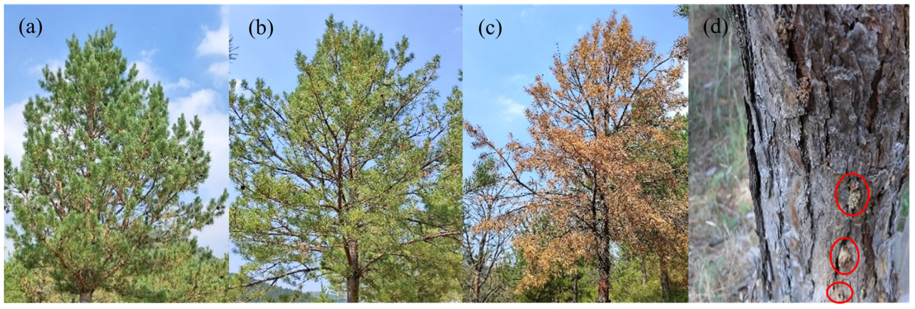
Ground data were collected in mid-July 2023. We conducted flight missions using a DJI Mavic 2 drone equipped with a Hasselblad camera with a 1-inch CMOS sensor and a 20-megapixel camera (DJI, Shenzhen, China) to obtain RGB orthophotos as reference data prior to the field survey. Subsequently, we conducted the field survey, including inspecting trunks for RTB entry holes (characterized by funnel-shaped resin masses) (Figure 2d). We also examined the canopy needles for any color changes. Based on the result, we categorized trees into three classes: healthy, infested (trees with green canopy needles but RTB entry holes on the trunks), and dead (trees with red canopy needles) (Figure 2).
The classification criteria and the number of samples used for subsequent research are shown in Table 1.

2.3. UAV-Based Thermal Infrared Image Acquisition and Processing

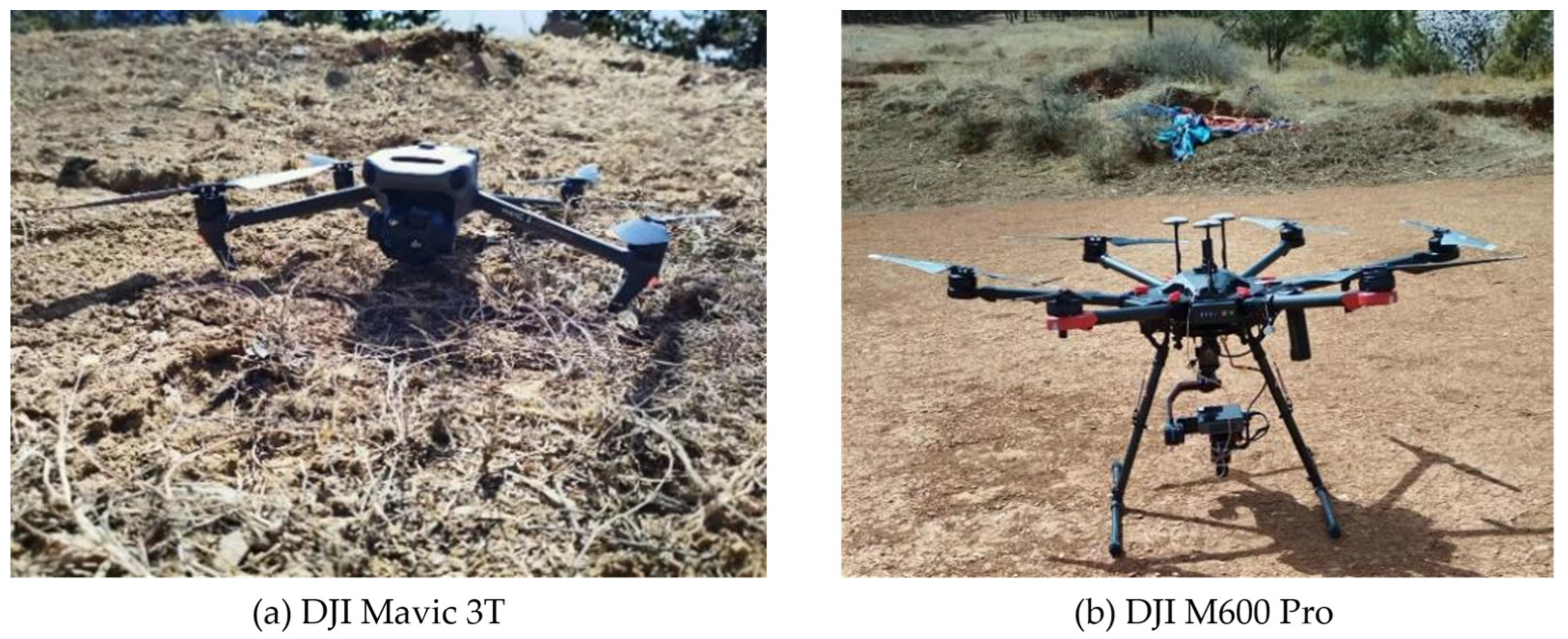
In September, we investigated the trees selected in July. Our investigation confirmed that there was no change in canopy color or any new beetle infestation compared with July. We captured thermal infrared images using a DJI Mavic 3T drone (DJI, Shenzhen, China, Figure 3a) equipped with a thermal infrared camera. The thermal camera model is M3T, featuring a 9 mm focal length and a temperature measurement range of −10 °C to 40 °C, with an uncooled vanadium oxide (Vox) sensor type. The images were taken on 17 September 2023, between 12:26 and 12:47 p.m., under clear skies, and with temperatures ranging from 10 °C to 27 °C. The flight altitude was set at 90 m. The primary flight line angle was 9°, with 90% front overlap and 90% side overlap. The infrared wavelength range is 8 µm to 14 µm, equivalent focal length is 40 mm, and pixel pitch is 12 µm. We used DJI Thermal Analysis Tool 3.0 software [34] to convert the acquired thermal infrared images (R-JPEG format, 16-bit) into grayscale images (selected from the color palettes) [35]. We used 0 to 255 grayscale levels to represent temperature variation range and imported these images into ENVI 5.6. Then, we segmented regions of interest to isolate individual tree canopies and obtained the canopy temperature (CT) based on the corresponding temperature thresholds.

2.4. UAV-Based Hyperspectral Image Acquisition and Processing

On 17 September 2023, from 12:00 to 12:40 noon, we acquired hyperspectral images using a DJI Matrice M600 Pro UAV (DJI, Shenzhen, China, Figure 3b). This drone was equipped with a Pika L hyperspectral camera (Resonon, Bozeman, MT, USA). The field of view was 17.6°, the focal length was 17 mm, and the flight altitude was 100 m. The flight included 50% forward and side overlap. The weather was sunny during the flight. A 3 m2 standard target was placed in the flight area for radiometric calibration and reflectance correction. The UAV’s inertial navigation and Z-survey i50 RTK were used to enhance POS accuracy. The raw hyperspectral data, including inertial navigation raw data bin files, were processed with differential technology using SBGcenter 3.4.89 software. Segmented Flight path data with Omap 10.0.5 software, pre-segmented with AirlineDivision 1.8 software, and the segmented data were input into the MegaCube 2.9.6.3 software. The maximum interpolation window was 10, ground elevation was 955 m, and spatial resolution was 5 cm. The images were geo-referenced in ArcMap 10.7, stitched and registered in ENVI Classic 5.6, and a hypercube was created in MegaCube 2.9.6.3. The hypercube was resampled and converted to reflectance imagery using the target fabric file. The obtained hyperspectral images included 150 spectral channels from 380 to 1016 nm, with a spectral resolution of approximately 4 nm.
To prepare canopy reflectance spectra data for the classification model, we used the ROI tool of ENVI 5.6 to delineate the crowns of single trees. A total of 106 trees were selected, with the number of trees at each stage shown in Table 1. For each tree, canopy reflectance spectra were extracted from ENVI 5.6. This study investigated three types of parameters: (1) canopy reflectance; (2) derivative analysis: derivatives are often used to enhance target features while reducing noise from factors such as lighting and soil background, thus improving stress detection capabilities [36,37]; (3) hyperspectral vegetation indices: these indices are formulated based on specific absorption features. The features quantify biophysical and biochemical indicators, aiding in the detection and differentiation of subtle variations in trees [38]. This study selected 27 spectral vegetation indices by reviewing the relevant literature and considering the features of the needles [11].The spectral vegetation indices are listed in Table 2.

2.5. Classification Models

2.5.1. Significance Analysis

We conducted a Kruskal–Wallis (K-W) analysis between the canopy reflectance of hyperspectral data obtained in Section 2.4 and the canopy temperature from Section 2.3 in IBM SPSS Statistics 25.0. We analyzed significant differences (p < 0.01) in the spectral reflectance, first derivative, and second derivative. Additionally, it was confirmed that 27 spectral vegetation indices and 1 canopy temperature parameter also exhibited significant differences. The data were divided into 5 single datasets and 4 combined datasets to be used as input variables for the random forest classification in the next section (Table 3).

2.5.2. Classification Model

This study used the random forest to establish a classification model with different input variables and compares the detection ability of different spectral features. Random forest is an ensemble learning classification algorithm. It was used in the analysis of remote sensing, suitable for solving multicollinearity problems with small sample sizes and multiple variables [54,55]. We constructed the random forest classification model in Python v3.11 using the “RandomForestClassifier” function from the “sklearn” package. The parameters were optimized through repeated code runs and ten-fold cross-validation, focusing on three parameters: the number of decision trees (n_estimators), the random seed in RandomForestClassifier (random_state), and the random seed in KFold (random_state). The parameter n_estimators was selected from 100, 200, and 500, with a stable state achieved around 100. The parameters random_state for RandomForestClassifier and KFold were adjusted around 47 and repeated until the optimal parameters were identified. This practice allows other researchers to validate and continue their work based on previous studies [56]. The dataset from Section 2.5.1 was used as input variables for the random forest. The random forest classifier was trained with the training dataset, and classification accuracy was evaluated using the test dataset. The data were randomly divided into training and test sets with a ratio of 70% to 30%.

2.5.3. Model Performance Evaluation

We assessed the performance of the classification model using the confusion matrix to compare predicted categories from the test set with ground truth categories. Equations (1)–(6) present commonly used metrics, including overall accuracy (OA), Cohen’s kappa coefficient, recall, precision, and F1 score, to evaluate the model’s performance [57,58]. These metrics provide insights into the model’s sensitivity, precision, and overall agreement with the ground truth.
R e c a l l = T P T P + F N
P r e c i s o n = T P T P + F P
F 1 s c o r e = 2 T P 2 T P + F P + F N
O A = T P + T N T P + T N + F P + F N
K a p p a = O A e A c c u r a c y 1 e A c c u r a c y
e A c c u r a c y = i = 1 k N p × N t S 2
OA and kappa were used to assess the general performance and consistency of the model beyond chance. Kappa measured the model’s agreement with the ground truth, providing a more robust evaluation of classification accuracy. Recall, precision, and F1 score evaluated the model’s effectiveness in detecting and distinguishing each category accurately. Recall measures the model’s ability to correctly identify positive instances, while precision assesses the proportion of true positive predictions out of all predicted positives. The F1 score then balances these two metrics into a single measure.

3. Results

3.1. Spectral Feature Difference Analysis

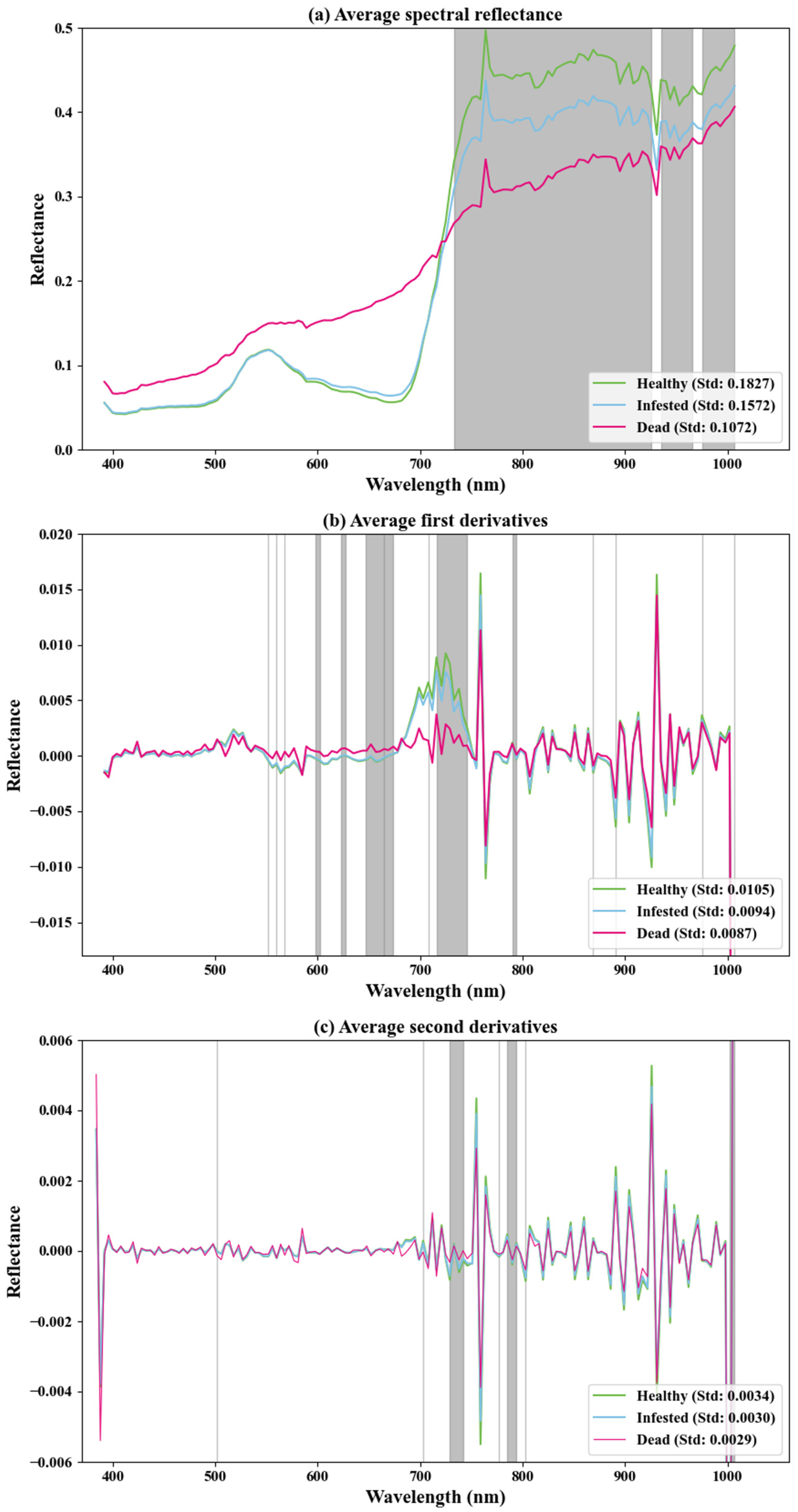
The spectral changes in three states were shown in Figure 4. Compared to infested and dead trees, healthy trees (green line) showed higher reflectance in the near-infrared region (760 nm to 1016 nm), reflecting the typical spectral characteristics of vegetation. The reflectance of infested trees showed little variation in the visible light region, with an overall trend similar to healthy trees. The spectral reflectance curve of dead trees differs markedly from that of healthy and infested trees, being higher in the visible light region and significantly lower in the near-infrared region. The K-W analysis showed significant differences in reflectance across 143 bands (p < 0.01) in three stages (Figure 4a). These differences were observed in the visible and near-infrared regions (657–686 nm and 729–1007 nm). A total of 61 bands (p < 0.01) between healthy and infested trees with differences were observed in near-infrared regions, particularly in the ranges of 733–926 nm, 935–966 nm, and 975–1007 nm.
The first and second derivatives reflect changes in the slope and concavity of the canopy spectral curve. The first derivative and second derivative curves of infested trees were similar to healthy trees (Figure 4b,c). The K-W analysis (p < 0.01) results showed that 24 first derivatives and 13 second derivatives differed between healthy and infested trees. Moreover, six first derivatives and seven second derivatives were in the near-infrared region, while the other derivatives were in the visible region. The dead trees showed significant changes across the entire spectral range.

3.2. Separability Analysis of SVIs and Temperature Parameters

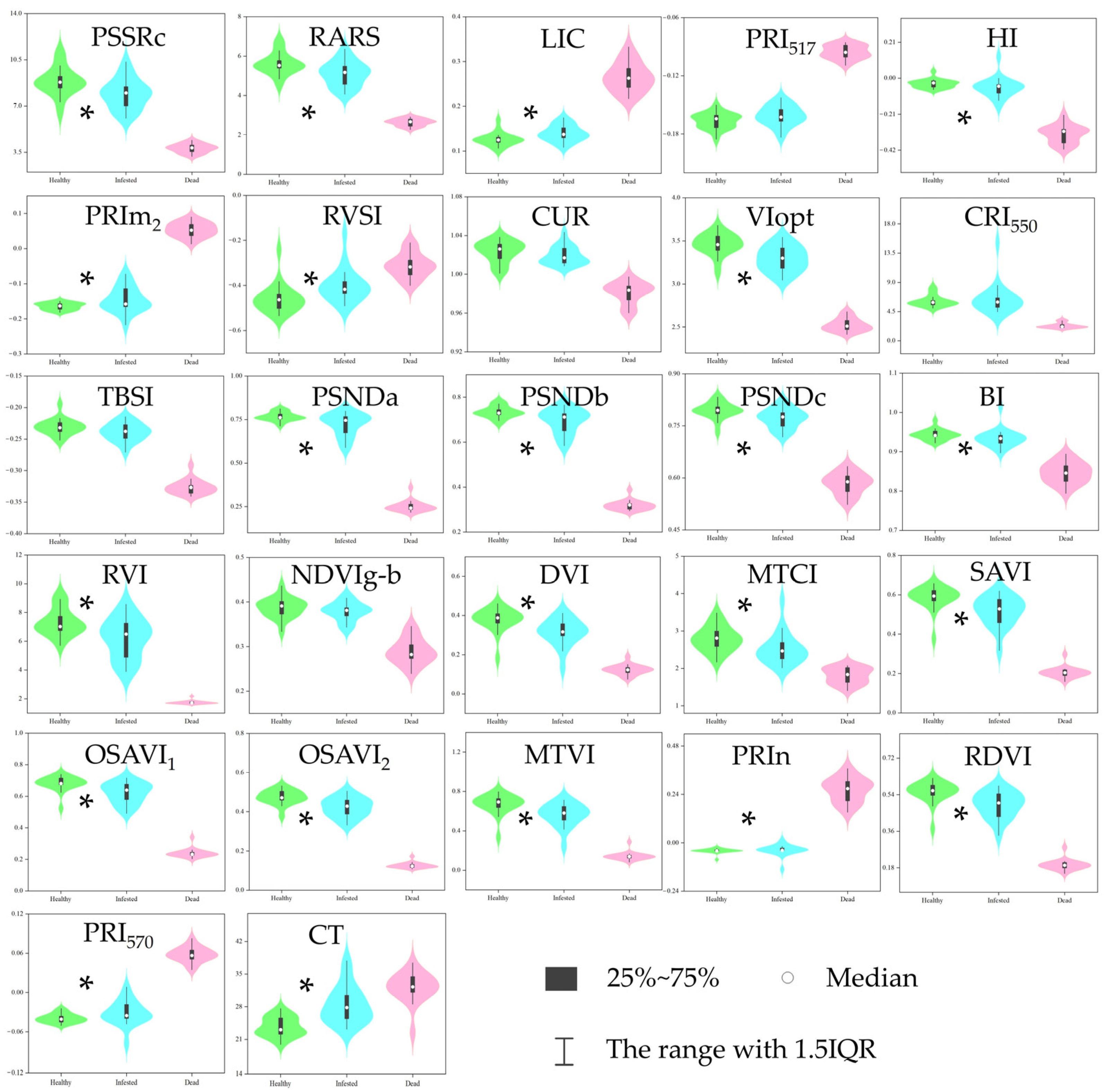
Violin plots showed the separability of 27 SVIs and temperature parameter (CT) across the three stages (Figure 5). The shape of the violin plots shows the probability density of the data, with wider sections indicating higher data concentration and narrower sections indicating greater dispersion. Kruskal–Wallis (K-W) analysis indicated that there were significant differences (p < 0.01) in 27 SVIs and the temperature parameter (CT) between healthy, infested, and dead trees. Almost all indices exhibited overlap between the 25th and 75th percentiles among the healthy and infested categories but showed minimal overlap with dead trees. Compared to healthy trees, infested trees showed significant differences (p < 0.01) in 21 SVIs and the temperature parameter (CT). The differences in PRI517, CUR, TBSI, PRIm4, NDVIg-b, and CRI550 were not significant. These SVIs were difficult to identify early RTB infestation.

3.3. RF Model Classification Results for Different Datasets

3.3.1. Classification Results Based on Single Dataset

We input five types of variables (SVIs, reflectance of bands, first derivative, second derivative, and the temperature parameter) with significant differences (p < 0.01) from Section 3.1 and Section 3.2 into the RF classifier to establish classification models. The number of input variables and the parameters optimized through ten-fold cross-validation (10-k CV) are shown in Table 4.
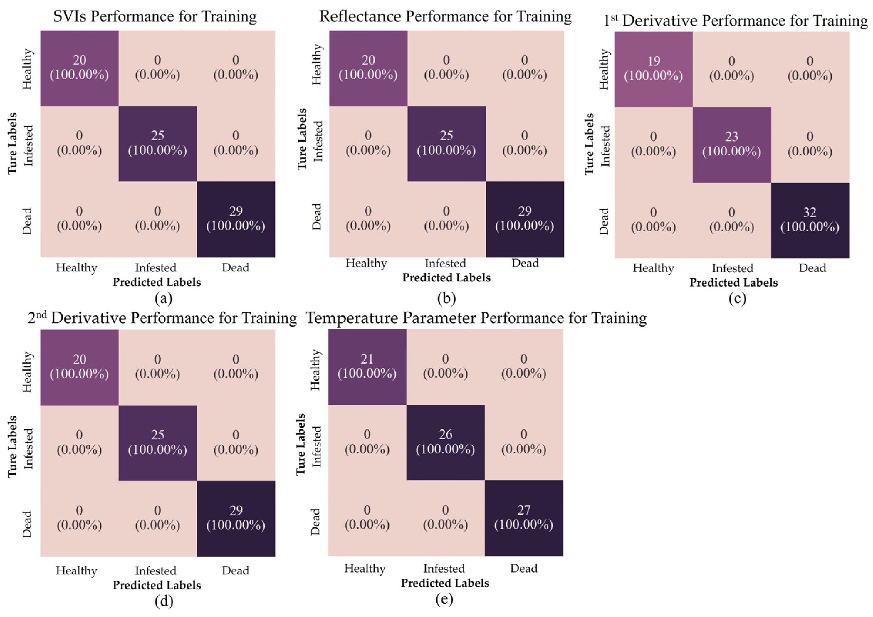
The single dataset’s performance on the training set is shown in Figure 6. All datasets demonstrated excellent classification performance, with precision and recall for each category reaching 100%. The confusion matrix showed non-zero elements only on the diagonal, indicating that the model correctly classified all training trees.
The classification results for the five single datasets in the RF model are shown in Figure 7. The results indicated that the model using SVIs as input variables performed the best, with an overall accuracy (OA) of 90.62% and a kappa coefficient of 0.86 followed by reflectance and the first derivative with OAs of 84.36% and 81.25%. The models using the second derivative and temperature parameter performed poorly, with OAs of 78.12% and 71.88%, respectively. The reduced overall accuracy for the second derivative was primarily due to misclassifications between healthy and infested trees. The temperature parameter had some misclassifications in both infested and dead stages, resulting in low overall accuracy.
The ability of different models to identify each health stage is shown in Figure 7 and Table 5. For dead trees, all datasets, except for the temperature parameter, could accurately detect it with recall and precision both reaching 100%, meaning that there were neither commission nor omission errors. Both recall and precision for the temperature parameter were 80%, indicating very few misclassifications. For infested trees, SVIs performed the best, with a precision and recall of 81.82% and 90%. Reflectance performed the second best, with a precision and recall of 72.73% and 80%. The first derivative’s precision reached 80%, but its recall was only 66.67%, representing that 33.33% of infested trees were misdiagnosed. The temperature parameter performed the worst, indicating that about half of the infested trees were either missed or misclassified. For healthy trees, SVIs performed the best, with a precision of 87.5%, recall of 77.78%, and F1 score of 82%, indicating that only 12.5% of healthy trees were misclassified as trees attacked by RTBs; 22.22% of healthy trees were misdiagnosed as attacked trees. The second derivative had the worst precision and recall of 60% and 66.67%, respectively.

3.3.2. Classification Results Based on Multiple Data Sources

In this section, we combined the four types of single datasets from Section 3.3 (SVIs, reflectance, first derivative, and second derivative) with the temperature parameter to create new combined dataset. Then, they were input into the RF classifier to build classification models. The input variables and parameters optimized through 10-fold cross-validation (10-k CV) are shown in Table 6.
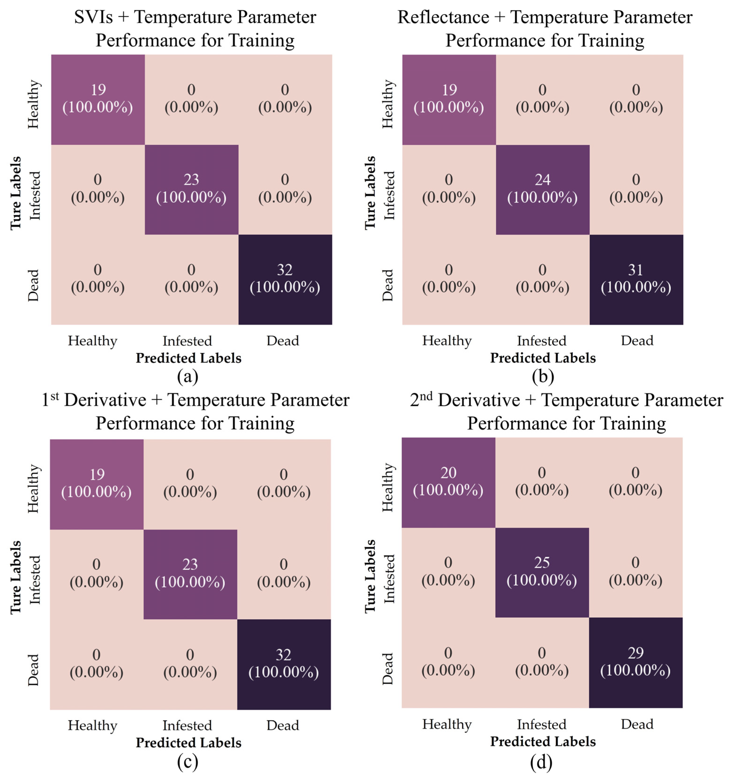
The combined dataset’s performance on the training set is shown in Figure 8. All datasets demonstrated excellent classification performance, with precision and recall for each category reaching 100%. The confusion matrix showed non-zero elements only on the diagonal, indicating that the model correctly classified all training trees.
The classification results of four combined datasets using the RF model were shown in Figure 9. All dataset’s OAs improved to some extent after adding the temperature parameter except R + T. S + T performed the best, with an OA of 93.75% and a kappa of 0.91. The model using 2D + T followed, with an OA of 90.62% and a kappa of 0.86. 1D + T and R + T showed lower performance, with OAs of 84.38% and 81.25% and a kappa of 0.76 and 0.72, respectively. The poor OA result was primarily due to misclassifications in the healthy and infested trees. In terms of accuracy improvement, combining thermal infrared temperature data led to the most significant increase with the 2D + T model, which improved by 18.74% compared to using the second derivative alone. S + T and 1D + T, respectively, had an increase of 3.13% and 3.11%, while the R + T showed a decrease of 3.11%.
The abilities of different models to identify each stage are shown in Figure 9 and Table 7. All combined datasets accurately identified dead trees with the precision reaching 100%. For infested trees, S + T had the highest evaluation metrics, with a recall and precision both of 91.67%, representing a 13.89% improvement in recall compared to the single dataset. The 2D + T performed the second best, with a recall of 80% and precision of 88.89%. 2D + T also showed the most significant increase in precision and recall, with improvement of 22.22% and 20%. For healthy trees, S + T achieved the best evaluation results. All the evaluation metrics reached 90%. 1D + T had the lowest recall (70.00%) and precision (77.78%).

4. Discussion

This study aimed to monitor individual infested trees using a combination of hyperspectral and thermal infrared data. The results showed that the trees’ spectral characteristics change following RTB infestation. By combining hyperspectral and temperature datasets, classification accuracy can be improved compared to using a single dataset alone.

4.1. Changes in Physiology and Spectra

Compared to healthy trees, infested trees’ reflectance decreased in the near-infrared region (760–1016 nm), with minimal changes in the visible region (400–760 nm) (Figure 4). This trend is consistent with previous studies on infestations of other bark beetles [11,22,23,24]. Changes in needle water content and other physiology substances (e.g., starch, proteins, lignin, and cellulose) possibly affect scattering, thereby altering reflectance in the near-infrared region [25]. Moreover, stomatal closure to conserve water might also contribute to reduced near-infrared reflectance [26]. Previous studies [22,25,59,60] suggest that needle pigment content changes in infested trees, especially chlorophyll degradation, leading to noticeable reflectance changes. These changes occur in the green peak (around 550 nm) and red edge (680–760 nm) regions. However, some studies have found that minor pigment changes might not be detectable spectrally. Previous research found that during the green attack stage, trees infested with the mountain pine beetle (MPB) did not have significant decreases in chlorophyll content. This means that low pigment content can saturate the spectral absorption features, making bands less sensitive to slight pigment changes [61,62]. This could explain the little changes in the visible spectral reflectance of pine trees infested by RTBs. Additionally, the differences in band changes might be influenced by the duration of the infestation. Gao et al. [21] collected data right after trees were infested by RTBs, while we acquired hyperspectral data after the trees had been infested for a longer period. Barta et al. [63] monitored bark beetle infestations using time-series HSI and found that bands related to chlorophyll absorption were affected first, followed by the near-infrared regions. The difference in data acquisition might explain the inconsistency in our findings.

4.2. Combination of Hyperspectral and Thermal Data

The results indicate that the temperature parameter can monitor trees attacked by RTBs. Why did the thermal infrared temperature parameter perform better in identifying healthy trees? Smiga et al. [64] observed that the stomatal closure in stressed plants can prevent water loss and leads to an increase in canopy temperature. Previous research indicated that thermal imaging shows that healthy trees have lower canopy temperatures than infested trees. This difference occurs due to the healthy trees maintaining effective transpiration cooling, while this effect is reduced in infested trees [65]. This finding aligns with our results and explains why the temperature parameter is effective in identifying healthy trees.
Hyperspectral data can also effectively monitor trees attacked by RTBs. The previous study [21] used airborne hyperspectral data to detect early infestations of P. tabuliformis by RTBs. The SVI-based RF model achieved an overall accuracy of 82.5% and a kappa of 0.74. For early-infested trees, it reached a precision of 77.78% and a recall of 70%. In contrast, our study’s SVI dataset achieved an overall accuracy of 90.62% and a kappa of 0.86. For early-infested trees, the precision was 81.82%, and the recall was 90%. Possible reasons for our results outperforming the previous study are as follows. The previous study used rectangular ROIs, which included background and shadow information. We used polygonal ROIs that followed the canopy edges, avoiding shadows and achieving better classification results. Sample size might also be an important factor. The previous study used 600 samples, while we used 106. A larger sample size could improve monitoring accuracy, but the appropriate sample size varies depending on the objectives and methods. In the previous study, shadows affected the data. As the sample size increased, the accumulated impact of these shadows reduced the accuracy. However, the optimal sample size still requires further experimentation. Additionally, the difference in tree species might contribute to the varying results. Our study was based on P. sylvestris var. mongolica, while the previous study focused on P. tabuliformis. Although the RTB infests both species, it is unclear which one it prefers. If the RTB prefers P. sylvestris var. mongolica, changes in attacked trees might be more pronounced compared to P. tabuliformis.
Hyperspectral features combined with temperature parameters improved the accuracy of all datasets. Among all combined datasets (a total of 106 samples), S + T had the highest OA at 93.75%, while 2D + T showed the greatest improvement in OA, increasing by 18.74% compared to 2D (Figure 9a,d). All combined datasets can accurately identify the 42 dead trees. For the 35 infested trees, S + T had the best identification performance, followed by 2D + T, which showed the greatest improvement (Table 7). SVIs were considered to be less affected by the influences of illumination and the background [66], while temperature changes were more sensitive to canopy changes caused by bark beetles. The combination of canopy temperature and SVIs enhanced classification performance [29]. Derivative analysis focuses on the shape of the spectral curves [36,37], resulting in poor identification of infested trees but accurate recognition of dead trees. The second derivative captured more subtle changes in the spectral curves. When these subtle changes were combined with temperature parameters, the model can better distinguish different classes. However, the OA of R + T decreased instead of increasing. The reason might be that there was some information overlap between reflectance and canopy temperature, which limited the combined model’s ability to gain significant new information from the temperature data. Additionally, the data combination method might also affect the model’s complexity and generalization ability. Inappropriate combinations of datasets might struggle to fully leverage their respective features, making it difficult to effectively train and generalize the model.

4.3. Limitations and Future Work

Although we achieved favorable results, further improvements are still necessary. As mentioned in Section 4.2, the sample size (106) was relatively small; a larger sample size typically enhances monitoring accuracy, but the appropriate sample size can vary depending on research objectives and methods. Future research will explore the optimal sample size and conduct experimental validation. The timing of data collection could also influence monitoring accuracy. We collected data after RTB infestation, while previous studies collected data shortly after trees were infested. The timing of data acquisition might affect changes in trees’ spectral characteristics. In the future, we will focus on multi-temporal monitoring to determine the optimal monitoring window period. While combining hyperspectral and thermal infrared data improved classification accuracy, a suboptimal data combination method could affect the model’s complexity and generalization ability. Some combinations (e.g., R + T) did not significantly improve classification performance, possibly due to information overlap between data sources or the combination method not fully utilizing each data source’s advantages. With the rapid development of remote sensing sensors and deep learning algorithms, future work will focus on integrating neural network algorithms to optimize data integration methods and enhance model performance. This aims to achieve more precise early monitoring of trees affected by infestation. We will also explore the potential of combining LiDAR and hyperspectral imagery for monitoring RTB, aiming to develop a detailed imaging monitoring system for infected trees.

5. Conclusions

This study combined UAV-based thermal infrared and hyperspectral data for monitoring P. sylvestris var. mongolica affected by the RTB. We classified trees into three classes: healthy, infested (green phase, where the RTB has invaded but the canopy remains green), and dead (red or gray phase), and we compared the performance of different spectral features and datasets. The main conclusions are as follows:
(1)
After RTB infestation, the spectral characteristics of canopies underwent significant changes. Compared to healthy trees, the spectral curves of dead trees showed significant declines in both the visible (400–760 nm) and near-infrared regions (760 nm to 1016 nm). The infested trees exhibited a noticeable decrease in the near-infrared region, while changes in the visible light region were subtle. All 27 SVIs and the CT used in this study were significantly different for dead trees, whereas 21 SVIs and the CT were significantly different for infested trees;
(2)
For single datasets, when reflectance, first derivatives, second derivatives, SVIs, and the temperature parameter were input into the random forest (RF) classifier, the SVIs dataset performed better than the others. For combined datasets, all datasets showed improved accuracy after combining the temperature parameter except R + T. S + T excelled in classifying RTB disturbances, achieving an overall accuracy (OA) of 93.75% from a total of 106 samples and a precision of 91.67% for the 35 early-infested trees. The OA of S + T is 3.13% higher than using the spectral vegetation index alone. This combination also significantly improved early detection precision by 13.89%. 2D + T showed the greatest improvement, with an OA improvement of 18.74% and a precision improvement of 22.22% for early-infested trees;
(3)
For the different stages of RTB infestation in trees, models using all datasets effectively identified dead trees. The temperature parameter showed potential in distinguishing between healthy and attacked trees (including early and dead stages). The combination of the HIS and TIR dataset performed well in distinguishing different stages.
The results indicated that UAV-based thermal infrared remote sensing could monitor RTB-infested P. sylvestris var. mongolica. Additionally, UAV-based hyperspectral and thermal infrared combined datasets also demonstrate potential in monitoring individual infested trees. The RF classification model using S + T could provide a reference for monitoring different stages of bark beetle infestation. Our findings demonstrated the applicability of UAV-based thermal infrared and combined hyperspectral datasets in monitoring RTB early-infested trees, providing important technical support for the scientific prevention and control of the RTB. With the rapid development of remote sensing sensors and deep learning algorithms, future efforts will focus on integrating these advanced algorithms and sensors to achieve more precise early monitoring of infested trees. Additionally, we will conduct multi-temporal monitoring of the RTB to identify the optimal detection window period.

Author Contributions

Conceptualization, L.Y.; methodology, P.B. and L.Y.; software, P.B.; validation, L.Y.; formal analysis, P.B.; investigation, P.B. and Y.L.; resources, Q.Z., J.K., and R.T.; writing—original draft preparation, P.B. and L.R.; writing—review and editing, L.Y. and L.R.; project administration, Y.L. All authors have read and agreed to the published version of the manuscript.

Funding

This research was funded by the National Key R & D Program of China (2022YFD1400400).

Data Availability Statement

The datasets presented in this article are not readily available because the data are part of an ongoing study. Requests to access the datasets should be directed to the authors.

Acknowledgments

The authors would like to thank the Ningcheng County Heilihe Forest Farm for their support in the field investigation.

Conflicts of Interest

The authors declare no conflicts of interest.

References

  1. Gao, B.; Ren, L.; Jiang, Q.; Liu, Y.; Yu, L.; Luo, Y. Geostatistical analysis of the spatial distribution of Dendroctonus valens in Pinus tabuliformis forests with different levels of infestation. Chin. J. Appl. Entomol. 2020, 57, 1427–1435. [Google Scholar]
  2. Wu, H.; Li, D.; Luo, Z.; He, S.; Jiang, S.; Song, Y. Disaster risk analysis of Dendroctonus valens in Northeast China. For. Pest Dis. 2022, 41, 22–28. [Google Scholar]
  3. Lu, X.; Chai, S.; Liu, H.; Jin, J.; Li, Z.; Xu, Z. The current situation and prevention and control countermeasures of forest and grass pests in the Three-North regions of China. For. Pest Dis. 2024, 43, 41–46. [Google Scholar]
  4. Song, Y.; Wu, H.; Song, L.; Du, W.; Zou, Y.; Dong, Y. Overview and countermeasures of invasive alien species in forest, grassland, and wetland ecosystems in Northeast China. For. Pest Dis. 2024, 43, 19–33. [Google Scholar]
  5. Li, Z.; Wang, B.; Li, Z.; Bai, G.; Wen, Y. Inner Mongolia focuses on managing invasive alien species. Inner Mongolia For. 2024, 69, 42–44. [Google Scholar]
  6. Liu, Y.; Gao, B.; Zhang, S.; Ren, L.; Luo, Y. Emergence and landing positions of Dendroctonus valens in Heilihe. Chin. J. Appl. Entomol. 2022, 59, 681–688. [Google Scholar]
  7. Foster, A.C.; Walter, J.A.; Shugart, H.H.; Sibold, J.; Negron, J. Spectral evidence of early-stage spruce beetle infestation in Engelmann spruce. For. Ecol. Manag. 2017, 384, 347–357. [Google Scholar] [CrossRef]
  8. Wulder, M.A.; Dymond, C.C.; White, J.C.; Leckie, D.G.; Carroll, A.L. Surveying mountain pine beetle damage of forests: A review of remote sensing opportunities. For. Ecol. Manag. 2006, 221, 27–41. [Google Scholar] [CrossRef]
  9. Zhan, Z.; Yu, L.; Li, Z.; Ren, L.; Gao, B.; Wang, L.; Luo, Y. Combining GF-2 and Sentinel-2 Images to Detect Tree Mortality Caused by Red Turpentine Beetle during the Early Outbreak Stage in North China. Forests 2020, 11, 172. [Google Scholar] [CrossRef]
  10. Liu, Y.; Gao, B.; Bian, L.; Ren, L.; Luo, Y. Invasion of Red Turpentine Beetles led to the increase of native trunk-boring beetles in Chinese pine stands. For. Ecol. Manag. 2024, 557, 121758. [Google Scholar] [CrossRef]
  11. Gao, B.; Yu, L.; Ren, L.; Zhan, Z.; Luo, Y. Early Detection of Dendroctonus valens Infestation with Machine Learning Algorithms Based on Hyperspectral Reflectance. Remote Sens. 2022, 14, 1373. [Google Scholar] [CrossRef]
  12. Zhang, J.; Huang, Y.; Pu, R.; Gonzalez-Moreno, P.; Yuan, L.; Wu, K.; Huang, W. Monitoring plant diseases and pests through remote sensing technology: A review. Comput. Electron. Agric. 2019, 165, 104943. [Google Scholar] [CrossRef]
  13. Franklin, S.; Wulder, M.; Skakun, R.S.; Carroll, A.L. Mountain pine beetle red-attack forest damage classification using stratified landsat TM data in British Columbia, Canada. Photogramm. Eng. Remote Sens. 2003, 69, 283–288. [Google Scholar] [CrossRef]
  14. Meddens, A.; Hicke, J.; Vierling, L.; Hudak, A.T. Evaluating methods to detect bark beetle-caused tree mortality using single-date and multi-date Landsat imagery. Remote Sens. Environ. 2013, 132, 49–58. [Google Scholar] [CrossRef]
  15. Immitzer, M.; Atzberger, C. Early Detection of Bark Beetle Infestation in Norway Spruce (Picea abies, L.) using WorldView-2 Data. Photogramm. Fernerkund. Geoinf. 2014, 5, 351–367. [Google Scholar] [CrossRef]
  16. Attard, M.R.G.; Phillips, R.A.; Bowler, E.; Clarke, P.J.; Cubaynes, H.; Johnston, D.W.; Fretwell, P.T. Review of Satellite Remote Sensing and Unoccupied Aircraft Systems for Counting Wildlife on Land. Remote Sens. 2024, 16, 627. [Google Scholar] [CrossRef]
  17. Adão, T.; Hruška, J.; Pádua, L.; Bessa, J.; Peres, E.; Morais, R.; Sousa, J. Hyperspectral Imaging: A Review on UAV-Based Sensors, Data Processing and Applications for Agriculture and Forestry. Remote Sens. 2017, 9, 1110. [Google Scholar] [CrossRef]
  18. Yu, R.; Luo, Y.; Li, H.; Yang, L.; Huang, H.; Yu, L.; Ren, L. Three-Dimensional Convolutional Neural Network Model for Early Detection of Pine Wilt Disease Using UAV-Based Hyperspectral Images. Remote Sens. 2021, 13, 4065. [Google Scholar] [CrossRef]
  19. Ma, Y.; Yang, B.; Zhao, N.; Zhang, X. Classification Diagnosis on the Damage Degree of Tomicus yunnanensis to Pinus yunnanensis Based on Hyperspectral and Airborne LiDAR. J. Southwest For. Univ. 2022, 42, 80–89. [Google Scholar]
  20. Lin, Q.; Huang, H.; Wang, J.; Chen, L.; Du, H.; Zhou, G. Early detection of pine shoot beetle attack using vertical profile of plant traits through UAV-based hyperspectral, thermal, and lidar data fusion. Int. J. Appl. Earth Obs. Geoinf. 2023, 125, 103549. [Google Scholar] [CrossRef]
  21. Gao, B.; Yu, L.; Ren, L.; Zhan, Z.; Luo, Y. Early Detection of Dendroctonus valens Infestation at Tree Level with a Hyperspectral UAV Image. Remote Sens. 2023, 15, 407. [Google Scholar] [CrossRef]
  22. Abdullah, H.; Darvishzadeh, R.; Skidmore, A.K.; Groen, T.A.; Heurich, M. European spruce bark beetle (Ips typographus, L.) green attack affects foliar reflectance and biochemical properties. Int. J. Appl. Earth Obs. Geoinf. 2018, 64, 199–209. [Google Scholar] [CrossRef]
  23. Liu, Y.; Zhan, Z.; Ren, L.; Ze, S.; Yu, L.; Jiang, Q.; Luo, Y. Hyperspectral evidence of early-stage pine shoot beetle attack in Yunnan pine. For. Ecol. Manag. 2021, 497, 119505. [Google Scholar] [CrossRef]
  24. Niemann, K.O.; Quinn, G.; Stephen, R.; Visintini, F.; Parton, D. Hyperspectral Remote Sensing of Mountain Pine Beetle with an Emphasis on Previsual Assessment. Can. J. Remote Sens. 2015, 41, 191–202. [Google Scholar] [CrossRef]
  25. Curran, P.J. Remote Sensing of Foliar Chemistry. Remote Sens. Environ. 1989, 30, 271–278. [Google Scholar] [CrossRef]
  26. Abdullah, H.; Skidmore, A.K.; Darvishzadeh, R.; Heurich, M. Timing of red-edge and shortwave infrared reflectance critical for early stress detection induced by bark beetle (Ips typographus, L.) attack. Int. J. Appl. Earth Obs. Geoinf. 2019, 82, 101900. [Google Scholar] [CrossRef]
  27. Wang, J.; Lin, Q.; Meng, S.; Huang, H.; Liu, Y. Individual Tree-Level Monitoring of Pest Infestation Combining Airborne Thermal Imagery and Light Detection and Ranging. Forests 2024, 15, 112. [Google Scholar] [CrossRef]
  28. Hais, M.; Kučera, T. Surface temperature change of spruce forest as a result of bark beetle attack: Remote sensing and GIS approach. Eur. J. For. Res. 2008, 127, 327–336. [Google Scholar] [CrossRef]
  29. Abdullah, H.; Darvishzadeh, R.; Skidmore, A.K.; Heurich, M. Sensitivity of Landsat-8 OLI and TIRS Data to Foliar Properties of Early Stage Bark Beetle (Ips typographus, L.) Infestation. Remote Sens. 2019, 11, 398. [Google Scholar] [CrossRef]
  30. Maes, W.H.; Huete, A.R.; Avino, M.; Boer, M.M.; Dehaan, R.; Pendall, E.; Griebel, A.; Steppe, K. Can UAV-Based Infrared Thermography Be Used to Study Plant-Parasite Interactions between Mistletoe and Eucalypt Trees? Remote Sens. 2018, 10, 2062. [Google Scholar] [CrossRef]
  31. Calderón, R.; Navas-Cortés, J.A.; Lucena, C.; Zarco-Tejada, P.J. High-resolution airborne hyperspectral and thermal imagery for early detection of Verticillium wilt of olive using fluorescence, temperature and narrow-band spectral indices. Remote Sens. Environ. 2013, 139, 231–245. [Google Scholar] [CrossRef]
  32. Wang, J.; Meng, S.; Lin, Q.; Liu, Y.; Huang, H. Detection of Yunnan Pine Shoot Beetle Stress Using UAV-Based Thermal Imagery and LiDAR. Appl. Sci. 2022, 12, 4372. [Google Scholar] [CrossRef]
  33. Smigaj, M.; Gaulton, R.; Suárez, J.C.; Barr, S.L. Combined use of spectral and structural characteristics for improved red band needle blight detection in pine plantation stands. For. Ecol. Manag. 2019, 434, 213–223. [Google Scholar] [CrossRef]
  34. Zhao, X. Monitoring of Pine Wilt Disease at Different Scales by Combining Thermal Infrared and Optical Remote Sensing Data. Master’s Thesis, Beijing Forestry University, Beijing, China, 31 May 2023. [Google Scholar]
  35. Sun, X. Study on Water Deficit of Walnut Forest Based on Infrared Thermography Information. Ph.D. Thesis, Chinese Academy of Forestry, Beijing, China, June 2019. [Google Scholar]
  36. Allen, B.; Dalponte, M.; Ørka, H.O.; Næsset, E.; Puliti, S.; Astrup, R.; Gobakken, T. UAV-Based Hyperspectral Imagery for Detection of Root, Butt, and Stem Rot in Norway Spruce. Remote Sens. 2022, 14, 3830. [Google Scholar] [CrossRef]
  37. Einzmann, K.; Atzberger, C.; Pinnel, N.; Glas, C.; Böck, S.; Seitz, R.; Immitzer, M. Early detection of spruce vitality loss with hyperspectral data: Results of an experimental study in Bavaria, Germany. Remote Sens. Environ. 2021, 266, 112676. [Google Scholar] [CrossRef]
  38. Clark, M.L.; Roberts, D.A. Species-Level Differences in Hyperspectral Metrics among Tropical Rainforest Trees as Determined by a Tree-Based Classifier. Remote Sens. 2012, 4, 1820–1855. [Google Scholar] [CrossRef]
  39. Blackburn, G.A. Spectral indices for estimating photosynthetic pigment concentrations: A test using senescent tree leaves. Int. J. Remote Sens. 2010, 19, 657–675. [Google Scholar] [CrossRef]
  40. Chappelle, E.W.; Kim, M.S.; McMurtrey, J.E., III. Ratio analysis of reflectance spectra (RARS): An algorithm for the remote estimation of the concentrations of chlorophyll a, chlorophyll b, and carotenoids in soybean leaves. Remote Sens. Environ. 1992, 39, 239–247. [Google Scholar] [CrossRef]
  41. Lichtenthaler, H.K.; Lang, M.; Sowinska, M.; Heisel, F.; Miehé, J.A. Detection of Vegetation Stress Via a New High Resolution Fluorescence Imaging System. J. Plant Physiol. 1996, 148, 599–612. [Google Scholar] [CrossRef]
  42. Gamon, J.A.; Peñuelas, J.; Field, C.B. A narrow-waveband spectral index that tracks diurnal changes in photosynthetic efficiency. Remote Sens. Environ. 1992, 41, 35–44. [Google Scholar] [CrossRef]
  43. Beck, P.; Zarco-Tejada, P.; Strobl, P.; San Miguel, J. The Feasibility of Detecting Trees Affected by the Pine Wood Nematode Using Remote Sensing; Publications Office of the European Union: Luxembourg, 2015; pp. 1831–9424. [Google Scholar]
  44. Gitelson, A.A.; Zur, Y.; Chivkunova, O.B.; Merzlyak, M.N. Assessing carotenoid content in plant leaves with reflectance spectroscopy. Photochem. Photobiol. 2002, 75, 272–281. [Google Scholar] [CrossRef] [PubMed]
  45. Merton, R.; Huntington, J. Early simulation results of the ARIES-1 satellite sensor for multi-temporal vegetation research derived from AVIRIS. In Proceedings of the Eighth Annual JPL Airborne Earth Science Workshop, Pasadena, CA, USA, 9–11 February 1999. [Google Scholar]
  46. Zarco-Tejada, P.J.; Miller, J.R.; Noland, T.L.; Mohammed, G.H.; Sampson, P.H. Scaling-up and model inversion methods with narrowband optical indices for chlorophyll content estimation in closed forest canopies with hyperspectral data. IEEE Trans. Geosci. Remote Sens. 2001, 39, 1491–1507. [Google Scholar] [CrossRef]
  47. Reyniers, M.; Walvoort, D.J.J.; De Baardemaaker, J. A linear model to predict with a multi-spectral radiometer the amount of nitrogen in winter wheat. Int. J. Remote Sens. 2007, 27, 4159–4179. [Google Scholar] [CrossRef]
  48. Tian, Y.-C.; Gu, K.-J.; Chu, X.; Yao, X.; Cao, W.-X.; Zhu, Y. Comparison of different hyperspectral vegetation indices for canopy leaf nitrogen concentration estimation in rice. Plant Soil. 2013, 376, 193–209. [Google Scholar] [CrossRef]
  49. Zhu, Y.; Yao, X.; Tian, Y.; Liu, X.; Cao, W. Analysis of common canopy vegetation indices for indicating leaf nitrogen accumulations in wheat and rice. Int. J. Appl. Earth Obs. Geoinf. 2008, 10, 1–10. [Google Scholar] [CrossRef]
  50. Dash, J.; Curran, P.J. The MERIS terrestrial chlorophyll index. Int. J. Remote Sens. 2010, 25, 5403–5413. [Google Scholar] [CrossRef]
  51. Gao, J.; Liang, T.; Yin, J.; Ge, J.; Feng, Q.; Wu, C.; Hou, M.; Liu, J.; Xie, H. Estimation of Alpine Grassland Forage Nitrogen Coupled with Hyperspectral Characteristics during Different Growth Periods on the Tibetan Plateau. Remote Sens. 2019, 11, 2085. [Google Scholar] [CrossRef]
  52. Wu, C.; Niu, Z.; Tang, Q.; Huang, W. Estimating chlorophyll content from hyperspectral vegetation indices: Modeling and validation. Agr. Forest Meteorol. 2008, 148, 1230–1241. [Google Scholar] [CrossRef]
  53. Haboudane, D. Hyperspectral vegetation indices and novel algorithms for predicting green LAI of crop canopies: Modeling and validation in the context of precision agriculture. Remote Sens. Environ. 2004, 90, 337–352. [Google Scholar] [CrossRef]
  54. Breiman, L. Random Forest. Mach. Learn. 2001, 45, 5–32. [Google Scholar] [CrossRef]
  55. Pal, M. Random forest classifier for remote sensing classification. Int. J. Remote Sens. 2007, 26, 217–222. [Google Scholar] [CrossRef]
  56. Pineau, J.; Vincent-Lamarre, P.; Sinha, K.; Larivière, V.; Beygelzimer, A.; d’Alché-Buc, F.; Fox, E.; Larochelle, H. Improving reproducibility in machine learning research: A report from the NeurIPS 2019 reproducibility program. J. Mach. Learn. Res. 2021, 22, 1–20. [Google Scholar]
  57. Cohen, J. A coefficient of agreement for nominal scales. Educ. Psychol. Meas. 1960, 20, 37–46. [Google Scholar] [CrossRef]
  58. Zhang, X.; Han, L.; Dong, Y.; Shi, Y.; Huang, W.; Han, L.; González-Moreno, P.; Ma, H.; Ye, H.; Sobeih, T. A Deep Learning-Based Approach for Automated Yellow Rust Disease Detection from High-Resolution Hyperspectral UAV Images. Remote Sens. 2019, 11, 1554. [Google Scholar] [CrossRef]
  59. Ahern, F.J. The effects of bark beetle stress on the foliar spectral reflectance of lodgepole pine. Int. J. Remote Sens. 2007, 9, 1451–1468. [Google Scholar] [CrossRef]
  60. Reichmuth, A.; Henning, L.; Pinnel, N.; Bachmann, M.; Rogge, D. Early Detection of Vitality Changes of Multi-Temporal Norway Spruce Laboratory Needle Measurements—The Ring-Barking Experiment. Remote Sens. 2018, 10, 57. [Google Scholar] [CrossRef]
  61. Mullen, K. Early Detection of Mountain Pine Beetle Damage in Ponderosa Pine Forests of the Black Hills Using Hyperspectral and WorldView-2 Data. Master’s Thesis, Minnesota State University, Mankato, MN, USA, 2016. [Google Scholar]
  62. Cheng, T.; Rivard, B.; Sánchez-Azofeifa, G.A.; Feng, J.; Calvo-Polanco, M. Continuous wavelet analysis for the detection of green attack damage due to mountain pine beetle infestation. Remote Sens. Environ. 2010, 114, 899–910. [Google Scholar] [CrossRef]
  63. Bárta, V.; Hanuš, J.; Dobrovolný, L.; Homolová, L. Comparison of field survey and remote sensing techniques for detection of bark beetle-infested trees. For. Ecol. Manag. 2022, 506, 119984. [Google Scholar] [CrossRef]
  64. Smigaj, M.; Gaulton, R.; Suárez, J.C.; Barr, S.L. Canopy temperature from an Unmanned Aerial Vehicle as an indicator of tree stress associated with red band needle blight severity. For. Ecol. Manag. 2019, 433, 699–708. [Google Scholar] [CrossRef]
  65. Lin, H.; Chen, Y.; Zhang, H.; Fu, P.; Fan, Z.; Watling, J. Stronger cooling effects of transpiration and leaf physical traits of plants from a hot dry habitat than from a hot wet habitat. Funct. Ecol. 2017, 31, 2202–2211. [Google Scholar] [CrossRef]
  66. Runesson, U.T. Considerations for Early Remote Detection of Mountain Pine Beetle in Green-Foliaged Lodgepole Pine. Ph.D. Thesis, University of British Columbia, Vancouver, BC, Canada, 1991. [Google Scholar]
Figure 1. Study area. (a) Chifeng City, Inner Mongolia Autonomous Region; (b) location of the study site.
Remotesensing 16 03840 g001
Figure 2. Symptoms of RTB infestation in pine trees canopy and trunk. (a) Canopy of the healthy trees; (b) canopy of the infested trees; (c) canopy of the dead trees; (d) symptoms of RTB infestation on the trunk, with red circles indicating RTB entry holes.
Remotesensing 16 03840 g002
Figure 3. UAV-based thermal infrared and hyperspectral systems. (a) DJI Mavic 3T; (b) DJI M600 Pro.
Remotesensing 16 03840 g003
Figure 4. Average canopy reflectance of trees. The green line, blue line, and red line, respectively, represent healthy, infested, and dead trees. The shaded gray area indicates significant differences between healthy and infested trees. (a) Average spectral reflectance; (b) average first derivative; (c) average second derivative.
Remotesensing 16 03840 g004
Figure 5. Spectral vegetation indices and temperature parameters for three stages. The symbol * indicates significant differences between healthy and infested trees.
Remotesensing 16 03840 g005
Figure 6. Overall performance and confusion matrix of random forest classification models using single datasets (training set). (a) SVIs; (b) reflectance; (c) first derivative; (d) second derivative; (e) temperature parameter.
Remotesensing 16 03840 g006
Figure 7. Overall performance and confusion matrix of random forest classification models using single datasets (test set). (a) SVIs; (b) reflectance; (c) first derivative; (d) second derivative; (e) temperature parameter.
Remotesensing 16 03840 g007
Figure 8. Overall performance and confusion matrix of random forest classification models using combined datasets (training set). (a) SVIs; (b) reflectance; (c) first derivative; (d) second derivative.
Remotesensing 16 03840 g008
Figure 9. Overall performance and confusion matrix of random forest classification models using combined datasets (test set). (a) SVIs; (b) reflectance; (c) first derivative; (d) second derivative.
Remotesensing 16 03840 g009
Table 1. The assessment indicators of pine health status and the number of samples.
ClassGrown ColorInfestation Symptoms of RTBsNumber of Samples
HealthyGreenNo29
InfestedGreenYes35
DeadRedYes42
Table 2. The spectral vegetation indices and temperature parameters.
IndexFormulation or DepictionRef.
Pigment-specific simple ratioPSSRc = R802/R472[39]
Pigment-specific normalized differencePSNDa = (R800 − R680)/(R800 + R680)
PSNDb = (R800 − R635)/(R800 + R635)
PSNDc = (R800 − R470)/(R800 + R470)
Ratio analysis of reflectanceRARS = R745/R513[40]
Lichtenthaler indexLIC = R439/R741[41]
Physiological reflectance indexPRI517 = (R517 − R534)/(R517 + R534)[42]
Photochemical reflectance
index
PRIm2 = (R600 − R534)/(R600 + R534)[43]
PRIm4 = (R570 − R531 − R670)/((R570 + R531 + R670)
PRIn = PRI570/[RDVI × (R700/R670)]
PRI570 = (R570 − R531)/(R570 + R531)
RDVI = (R800 − R670)/(R800 + R670)0.5
Carotenoid reflectance indexCRI550 = 1/R510 − 1/R550[44]
Red-edge vegetation stress indexRVSI = (R715 − R754)/2 − R732[45]
Curvature indexCUR = R677 × R690/R6852[46]
Health indexHI = (R534 − R698)/(R534 + R698) − R702/2[43]
Optimal vegetation indexVIopt = 1.45 × (R8022 + 1)/(R668 + 0.45)[47]
Three-band spectral indexTBSI = (R605 − R521 − R681)/(R605 + R521 + R681)[48]
Blue indexBI = R450/R490[43]
Ratio vegetation indexRVI = R810/R660[49]
Normalized difference vegetation indexNDVIg−b = (R537 − R440)/(R537 + R440)[48]
Difference vegetation indexDVI = R810 − R680[49]
MERIS terrestrial chlorophyll indexMTCI = (R754 − R709)/(R709 − R681)[50]
Soil-adjusted vegetation indexSAVI = (1 + 0.5) × [(R800 − R670)/(R800 + R670 + 0.5)][51]
Optimized soil-adjusted vegetation indexOSAVI1 = (1 + 0.16) × [(R800 − R670)/(R800 + R670 + 0.16)][52]
OSAVI2 = (1 + 0.16) × [(R750 − R705)/(R750 + R705 + 0.16)]
Modified triangular vegetation indexMTVI = 1.2 × [1.2 × (R800 − R550) − 2.5 × (R670 − R550)][53]
Canopy temperatureCT[34]
Table 3. Model input variables.
Data TypeVariablesData TypeVariables
Single datasetReflectanceCombined datasetReflectance + Temperature parameter
Single dataset1st derivativeCombined dataset1st derivative + Temperature parameter
Single dataset2nd derivativeCombined dataset2nd derivative + Temperature parameter
Single datasetVegetation indicesCombined datasetVegetation indices + Temperature parameter
Single datasetTemperature parameter
Table 4. Parameters of the RF models with a single dataset (n_Estimators = 100).
AbbreviationInput
Variables
Number of VariablesParameters
Random_State of Train_Test_SplitRandom_State of 10-Kfold
SSVIs274249
RReflectance of bands1434246
1D1st derivative1164646
2D2nd derivative1004249
TTemperature parameter14849
Table 5. Evaluation metrics for each class of single dataset.
AbbreviationInputOAKappaClassPrecision (%)Recall (%)F1-Score (%)
SSVIs90.620.86Healthy87.577.7882
Infested81.829086
Dead100100100
RReflectance of bands84.380.76Healthy85.7166.6775
Infested72.738076
Dead92.8610096
1D1st
derivative
81.250.72Healthy66.678073
Infested8066.6773
Dead100100100
2D2nd
derivative
78.120.67Healthy6066.6763
Infested66.676063
Dead100100100
TTemperature parameter71.880.56Healthy85.717580
Infested5055.5653
Dead808080
Table 6. Parameters of the RF models with combined dataset (n_Estimators = 100).
AbbreviationInput VariablesNumber of VariablesParameters
Random_State of Train_Test_SplitRandom_State of 10-Kfold
S + TSVIs + Temperature parameter284648
R + TReflectance of bands +
Temperature parameter
1444748
1D + T1st derivative +
Temperature parameter
1174642
2D + T2nd derivative + Temperature parameter1014242
Table 7. Evaluation metrics for each class of combined dataset.
AbbreviationInputOAKappaClassPrecision (%)Recall (%)F1-Score (%)
S + TSVIs + Temperature parameter93.750.91Healthy909090
Infested91.6791.6791.67
Dead100100100
R + TReflectance of bands + Temperature parameter81.250.72Healthy808080
Infested69.2381.8275
Dead10081.8290
1D + T1st
derivative + Temperature parameter
84.380.76Healthy77.787074
Infested76.9283.3380
Dead100100100
2D + T2nd
derivative + Temperature parameter
90.620.86Healthy8088.8984
Infested88.898084
Dead100100100
Disclaimer/Publisher’s Note: The statements, opinions and data contained in all publications are solely those of the individual author(s) and contributor(s) and not of MDPI and/or the editor(s). MDPI and/or the editor(s) disclaim responsibility for any injury to people or property resulting from any ideas, methods, instructions or products referred to in the content.