Article

Remote Sensing Image Denoising Based on Feature Interaction Complementary Learning

School of Aerospace Science and Technology, Xidian University, Xi’an 710126, China
*
Author to whom correspondence should be addressed.
Remote Sens. 2024, 16(20), 3820; https://doi.org/10.3390/rs16203820
Submission received: 29 July 2024 / Revised: 8 September 2024 / Accepted: 18 September 2024 / Published: 14 October 2024

Abstract

:
Optical remote sensing images are of considerable significance in a plethora of applications, including feature recognition and scene semantic segmentation. However, the quality of remote sensing images is compromised by the influence of various types of noise, which has a detrimental impact on their practical applications in the aforementioned fields. Furthermore, the intricate texture characteristics inherent to remote sensing images present a significant hurdle in the removal of noise and the restoration of image texture details. In order to address these challenges, we propose a feature interaction complementary learning (FICL) strategy for remote sensing image denoising. In practical terms, the network is comprised of four main components: noise predictor (NP), reconstructed image predictor (RIP), feature interaction module (FIM), and fusion module. The combination of these modules serves to not only complete the fusion of the prediction results of NP and RIP, but also to achieve a deep coupling of the characteristics of the two predictors. Consequently, the advantages of noise prediction and reconstructed image prediction can be combined, thereby enhancing the denoising capability of the model. Furthermore, comprehensive experimentation on both synthetic Gaussian noise datasets and real-world denoising datasets has demonstrated that FICL has achieved favorable outcomes, emphasizing the efficacy and robustness of the proposed framework.

Graphical Abstract

1. Introduction

Remote sensing is a technology that employs non-contact data collection to obtain information about the Earth [1]. Its applications are diverse, encompassing environmental monitoring [2], military target recognition [3], moving target tracking [4], resource exploration [5], and other fields [6,7]. Nevertheless, the remote sensing imaging process, coupled with storage, compression, and transmission procedures, is prone to introducing random signals that degrade image quality. Consequently, optical remote sensing images are frequently plagued by noise signals, which not only hinder human visual interpretation but also significantly compromise the accuracy of subsequent image processing tasks [8]. This limitation falls short of fulfilling the growing demand for high-quality remote sensing data.
Traditional image noise reduction approaches frequently employ intricate algorithms tailored to rejuvenate deteriorated images, grounded on specific noise models. These encompass non-local self-similarity (NSS) [9], sparse representation methods [10], gradient-based techniques [11], Markov random field (MRF) modeling [12], and external denoising priors [13,14]. Among these, the block-matching and 3D filtering (BM3D) [9] and weighted nuclear norm minimization (WNNM) [10] models are exemplary model-driven strategies. In the field of remote sensing image denoising there are Non-local Meets Global (NLMG) based on non-local low-rank tensor approximation [15], spatial domain spectral residual total variation (SSRTV) based on three-dimensional full variational (3DTV) regularization [16], and asymmetric noise modelling based on bandwidth-directed asymmetric Laplacian (AL) distribution [17]. While adept at mitigating additive white Gaussian noise (AWGN) with predefined noise levels, these methods confront limitations, including protracted computational demands, challenges in suppressing spatially varying noise patterns, and shortcomings in intricately restoring fine image details [18,19].
In recent times, deep learning [20] has garnered immense popularity across diverse domains, encompassing object detection [21,22], anomaly detection [23,24], and co-saliency detection [25,26], among others [27]. Similarly, this cutting-edge technology has permeated the realm of image denoising, ushering in novel advancements. Zhang et al. pioneered the development of denoising convolutional neural networks (DnCNNs) [28], followed by the introduction of fast and flexible denoising networks (FFDNet) [29]. To enable better removal of real-world image noise, Guo et al. [30] proposed CBDNet, which embeds a noise estimation subnetwork with asymmetric learning to improve generalization and allow interactive denoising improvements. Moreover, Saeed Anwar and Nick Barnes made a significant contribution with the development of RIDNet, a pioneering single-stage blind real-world image denoising network [31]. Chang et al. [32] contributed yet another significant advancement with their spatial-adaptive denoising network (SADNet), designed for efficient and effective single image blind noise removal. Han et al. [33] proposed a novel remote sensing image denoising network (RSIDNet), which uses an attention mechanism to improve the denoising effect of the network. Xu et al. [34] present a new depth expansion multiscale regularization network (DUMRN) for image denoising. Jian et al. [35] proposed a dual-complementary convolution network (DCCNet), comprising a structural and a detailed subnetwork, for the purpose of repairing the structural and detailed deficiencies of noisy remote-sensing images. Wu et al. [36] proposed a nonlocal local perceptual network (NLANe) combining local and nonlocal self-similarity prior guidance to remove noise in eigen-images.
Generation adversarial network (GAN), it has become one of the mainstream algorithms for denoising due to its excellent performance. The earliest GAN is proposed by Goodfellow et al. [37], and it is based on the discriminator and generator. The GAN comprises a discriminator (D) that differentiates real from generator (G)-produced images, and a G that learns to deceive D with realistic images. This competition suppresses the denoising blur, enhancing image quality. To improve the denoising capabilities of GANs, Zhu et al. [38] implemented a robust GAN-based denoising network that incorporates global residuals in the generator and uses an optimization algorithm to train and optimize the noise, achieving significant denoising performance with high accuracy. Chen et al. [39] further developed a Wasserstein Generative Adversarial Network (WGAN)-based training framework for image denoising, applying it to the enhancement of cell image quality. Meanwhile, Lyu et al. [40] leveraged a Generative Adversarial Network-based denoising model, DeGAN, to remove muti-noise from images. Wang et al. [41] proposed an innovative blind image denoising approach utilizing an Asymmetric Generative Adversarial Network (ID-AGAN), focusing on optimizing the denoising of multi-dimensional image data. Pan et al. [42] developed a global residual generation adversarial network (GR-GAN), which realized rock slice image denoising by optimizing the residual structure and loss function. Huang et al. [43] introduced an unsupervised learning technique for speckle reduction in optical coherence tomography (OCT) images, utilizing disentangled representation and generative adversarial network (DRGAN). Han et al. [44] proposed a coarse-to-fine multi-scale feature hybrid low-dose CT denoising network CMFHGAN, which effectively improves the denoising performance by global denoising, local texture feature enhancement and self-calibrated feature fusion, combined with a multi-resolution initial discriminator. Zheng et al. [45] introduced Dehaze-AGGAN for unpaired remote sensing image dehazing that utilizes enhanced attention-guided generative adversarial networks to effectively restore clear images from hazy inputs. Chen et al. [46] created a memory-oriented generative adaptive network (MO-GAN) for single remote sensing image defogging. This method introduces a memory mechanism to guide the defogging process, and can restore clear remote sensing images without matching clear images. Jin et al. [47] proposed a remote sensing image cloud removal method based on Hybrid Attention Generative Adversarial Network (HyA GAN), which guides the model to generate clear and cloud free remote sensing images by combining multiple attention mechanisms. Kas et al. [48] proposed a degradation level-based learnable generative adversarial network (DLL-GAN), which improves performance in image enhancement tasks such as super-resolution, denoising, and JPEG artefact removal by introducing a degradation estimation loss function based on convolutional neural networks.
Among the aforementioned methods, some focus exclusively on reducing noise in artificially synthesized data, resulting in limited effectiveness when dealing with real-world noise. While several approaches do address real-world image denoising, they typically either train to reconstruct the denoised image directly, or first identify the noise and then remove it from the noisy image to derive the denoised result. Geng et al. [49] posit that both content learning and noise learning have distinct advantages and that a combination of the two is optimal. Accordingly, they put forth a content-noise complementary learning (CNCL) strategy specifically for denoising medical images in the image domain. Zhao et al. [50] developed a modular complementary learning strategy based on GAN, the dual-GAN complementary learning (DGCL) strategy. Although the CNCL and DGCL methods use two predictive models to concurrently learn the image content and the noise in a synergistic fashion, thereby enhancing the learning outcome compared to the use of a solitary predictor, they simply fuse the prediction results of the two predictors without deeper feature-level coupling. In addition, both CNCL and DGCL are based on the GAN, which is not easy to train.
In view of the aforementioned discussion, to solve these problems, a feature interactive complementary learning (FICL) model for remote sensing image denoising is proposed. The denoising model not only realizes the fusion of the results generated by the image predictor and the noise predictor, but also realizes the coupling of the characteristics of the two predictors. This denoising model improves the quality of the final denoised image and the training process is simpler compared to the previous complementary learning. We validate the proposed model on synthetic Gaussian noise datasets and real-world denoising datasets. The experimental results show that the method produces higher quality denoised images.
In conclusion, the principal works of this article are as follows:
  • We proposed a remote sensing image denoising model based on feature interaction complementary learning, which we term the FICL model. The FICL model is comprised of four distinct components: reconstructed image predictor (RIP), noise predictor (NP), feature interaction module (FIM), and fusion module. The model’s original fusion of results also allows for the coupling of features, more fully integrating the strengths of both paradigms.
  • We proposed an FIM which facilitates the interaction between the features of the reconstructed image and noise, thereby enhancing the denoising efficacy of the network.
  • The proposed FICL model was evaluated on both synthetic Gaussian noise datasets and existing real-world denoising datasets. In comparison with other, more advanced techniques, the FICL method demonstrates superior performance.

2. Materials and Methods

In this part, we first outline the complementary learning strategy, and then expound our proposed FICL model based on complementary learning. Finally, the loss function of the network is described.

2.1. Complementary Learning

Within the realm of digital image processing, it is a common assumption that the signal and the noise are considered to be statistically independent. This implies that the final signal waveform is the result of the superposition of both the signal and the noise:
y = x + n
where x is a noiseless image, y is an image polluted by noise and n is the noise. There are two predictors, p 1 and p 2 , where p 1 is used to predict the reconstructed image and p 2 is used to predict the noise then the reconstructed image is indirectly obtained according to Equation (1). Complementary learning is the fusion of the reconstructed image obtained by the two predictors. Thus, complementary learning can be expressed as:
f i n a l i m a g e = f u s i o n ( p 1 ( y ) , y p 2 ( y ) )
Both reconstructed image prediction and noise prediction have significant advantages in image denoising. Reconstructed image prediction demonstrates a more stable performance in noise cancellation [51], while noise prediction proves beneficial in preventing performance degradation and preserving image structures [52]. By leveraging these complementary strengths, more effective denoising model can be devised.

2.2. Feature Interaction Complementary Learning

The FICL model is shown in Figure 1, which consists of four parts: RIP, NP, FIM, and fusion module. The RIP is built via incorporating multi-scale ResNet (MSResNet) and convolutional block attention module (CBAM) into the traditional Unet architecture, which is employed to obtain the reconstructed image directly. The NP is built upon the classic Unet framework, which functions by estimating the noise present in an image and subsequently removing this estimated noise from the noisy image, thereby revealing a denoised version. The FIM allows interaction between the features of the reconstructed image and the noise in the encoder to obtain complementary features. The fusion module, which consists of a 1 × 1 convolution, combines the reconstructed images predicted by the RIP and NP to obtain the final reconstructed image.

2.2.1. Reconstructed Image Predictor

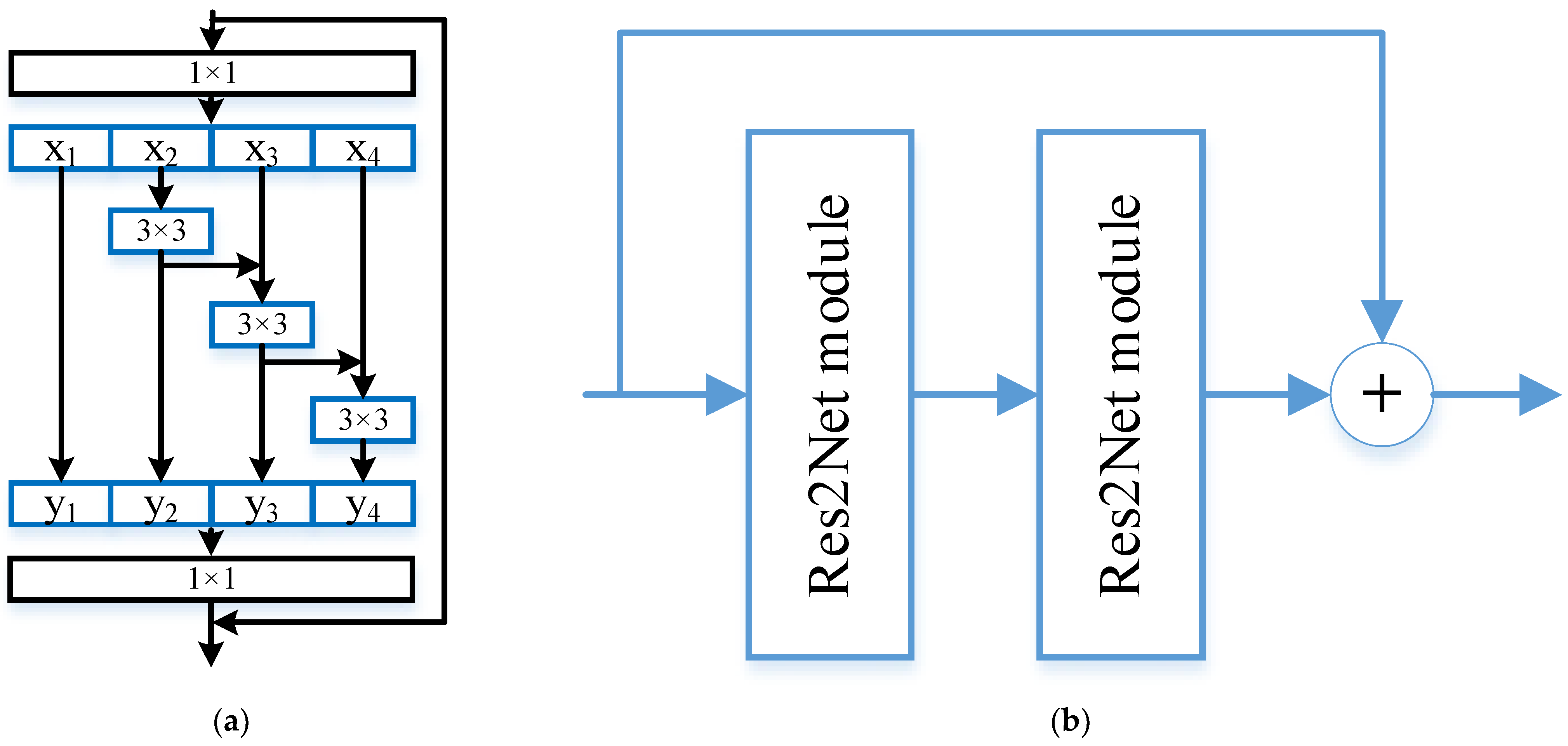
We use the improved Unet network using multi-scale method and CBAM as the reconstructed image predictor. Res2Net [53] enhances ResNet [54] with multi-scale features at a finer level, using hierarchical residual connections within blocks. It widens receptive fields and boosts performance. Combining two Res2Net modules like ResNet creates MSResNet, further expanding receptive fields. See Figure 2 for the module design.
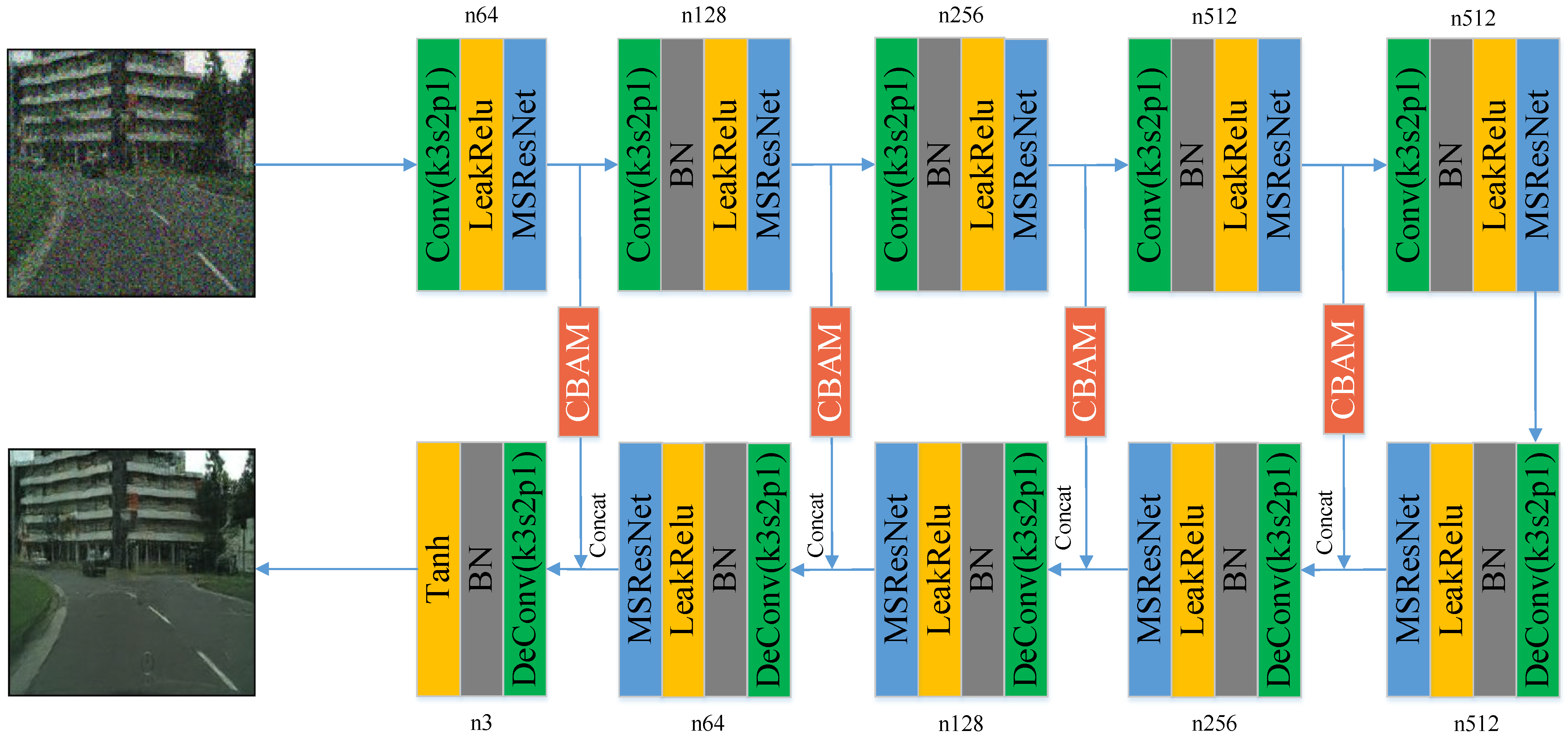
As illustrated in Figure 3, the MSResNet module is strategically inserted after each downsampling and upsampling stage within the Unet framework [55]. Both the convolutional and deconvolutional operations for these processes utilize a kernel size of 3, accompanied by a stride of 2 and padding of 1. Given the presence of redundant information in the original image, a direct flow of the downsampled feature maps through Unet’s skip-connections could hinder efficient image reconstruction. To address this, the CBAM (Convolutional Block Attention Module) [56], an effective CNN attention mechanism, is introduced and incorporated into the skip-connections of the generator Unet. This refinement helps to filter out irrelevant features and prioritize the most crucial information for improved reconstruction results.

2.2.2. Noise Predictor

Due to the characteristics of noise signal, we use the ordinary Unet network as the noise predictor. As shown in Figure 4, we use convolution and deconvolution with convolution kernel of 4 × 4 and step size of 2 as the encoder and decoder of Unet network.

2.2.3. Feature Interaction Module

NP feature and RIP feature interact as shown in Figure 5, where a Conditional Weight Generator (CWG) is composed of an average pooling layer, a full connection layer, and a sigmoid layer in turn. Coupled NP feature and RIP feature are feature graphs after interaction. Mid NP feature and RIP feature are middle feature images generated after multiplication. The expression of the whole feature interaction process is as follows:
M i d N P F e a t u r e = N P F e a t u r e × C W G ( N P F e a t u r e ) × C o n v 1 × 1 ( R I P F e a t u r e )
M i d R I P F e a t u r e = R I P F e a t u r e × C W G ( R I P F e a t u r e ) × C o n v 1 × 1 ( N P F e a t u r e )
C o u p l e d N P F e a t u r e = N P F e a t u r e M i d N P F e a t u r e + M i d R I P F e a t u r e
C o u p l e d R I P F e a t u r e = R I P F e a t u r e M i d R I P F e a t u r e + M i d N P F e a t u r e

2.2.4. Fusion Module

The fusion module consists of a 1 × 1 convolution. As shown in Figure 6, The results of the two predictors are connected first and then input to the fusion module. The fusion module fuses the two predicted images and outputs the final denoised image.

2.3. Loss Functions

As can be seen from Section 2.2, we need to conduct supervised learning on the output results of the two predictors and the final fused image. Therefore, the loss of FICL L F I C L can be expressed as:
L F I C L = L f i n + λ L n o i s e + μ L r s i m a g e
where L n o i s e is the loss of noise predictor, λ is the loss weight of L n o i s e , L r s i m a g e is the loss of reconstructed image predictor, μ is the loss weight of L r s i m a g e , L f i n is the loss of the fusion of two predictor results, L n o i s e can be written as:
L n o i s e = L c h a r n + φ L a s y m m
where L c h a r n is Charbonnier loss [57] between the predicted noise pren and the ground-truth noise gtn, L a s y m m is asymmetric loss on noise estimation [30], φ is the loss weight of L a s y m m , L c h a r n and L a s y m m expressions are shown in Equations (9) and (10):
L c h a r n = ( p r e n g t n ) 2 + ε 2
L a s y m m = i α II ( p r e n g t n ) < 0 ( p r e n g t n ) 2
where the constant ε is set as 10−3, constant α is set as 0.3. Both L r s i m a g e and L f i n are both loss functions between the reconstructed image prei and the ground-truth image gti, which can be expressed as
L r s i m a g e a n d L f i n = L c h a r i + η L S S I M + ν L e d g e
where L c h a r i is Charbonnier loss between the reconstructed image prei and the ground-truth image gti, where L S S I M is a loss function on the structural similarity(SSIM) [58] value between reconstructed image and ground truth, where η is the loss weight of L S S I M , ν is the loss weight of L e d g e , SSIM is an indicator that quantifies the resemblance between a pair of images, scoring within the range of −1 to 1. L S S I M can be written as:
L S S I M = 1 S S I M ( p r e i , g t i )
L e d g e in (11) is the edge loss [59], which can maintain high-frequency structure information better. The L e d g e can be denoted as:
L e d g e = Δ p r e i Δ g t i 2 + ε 2
where the Δ denotes the Laplacian operator [60], and the constant ε is set as 10−3.

3. Experiments and Results

In this section, we elaborate on the extensive experimental endeavors undertaken to verify the efficacy and superiority of the proposed methodology.

3.1. Datasets and Evaluation Metrics

3.1.1. Datasets

The creation of denoising datasets primarily encompasses two distinct methodologies:
  • Leveraging existing high-quality images from image databases, these images undergo image processing techniques, encompassing linear transformations, brightness adjustments, among others. Subsequently, synthetic noise is meticulously added in accordance with a predefined noise model, thereby generating noise-corrupted images.
  • Multiple images of the same scene are continuously captured. Following this, rigorous image processing procedures are implemented, including image registration and the removal of anomalous images. Ultimately, a weighted average of these processed images is computed to synthesize a ground truth image, serving as the reference for denoising tasks.
Method 1 is straightforward and efficient, allowing for precise control over the level of noise. Therefore, we use the NWPU-RESISC45 dataset to add AWGN with the σ∈[0, 60] for training and testing. In order to verify the denoising effect of the trained model on other datasets, we randomly selected some images from the UCMerceded_LandUse dataset as the test set. The denoising effect of the network trained on this dataset on real noisy images is limited. Method 2 requires capturing a large number of images, which is relatively labor-intensive but more closely aligned with the actual denoising requirements in the real-world. Due to the lack of denoising datasets based on Method 2 in remote sensing images, we use the typical datasets PolyU and SIDD (Smartphone Image Denoising Dataset) of Method 2 to detect the denoising capabilities of all methods in the real-world.
The NWPU-RESISC45 [61] remote sensing dataset is a large-scale public dataset published by Northwestern Polytechnical University for the purpose of remote sensing image scene classification. It contains 45 distinct categories of scenes. The dimensions of each remote sensing image in the dataset are 256 × 256. A total of 70 images were randomly selected from each scene, with 60 images being allocated to the training dataset and the remaining 10 images being designated for the testing dataset.
The UCMerced_LandUse [62] remote sensing dataset is a publicly accessible repository of remote sensing image scene classification data, comprising 21 distinct scene types, released by the University of California. The dimensions of each remote sensing image in the dataset are 256 pixels in both the horizontal and vertical directions. A supplementary test dataset was constructed by randomly selecting 10 images from each scene.
The PolyU dataset [63], a real-world collection, comprises images captured by five cameras in 40 diverse scenes, each scene featuring a matching pair of noisy and clean images. For the experiments, 32 scenes were randomly picked from this dataset, and their images were cropped to 256 × 256 pixels. Following that, a selection of 2000 of the cropped images was designated for the training dataset, and an additional 400 images, extracted from the remaining scenes, were set aside to form the test dataset.
The SIDD [64], a comprehensive collection of real-world photographs, initially consists of 200 sets of paired noisy and pristine images. Out of this original collection, a subset of 160 distinct scenes was extracted and resized to 256 × 256 pixels for the training purposes, amassing a total of 2462 individual scenes within the training dataset. The remaining 40 scenes were similarly resized, and from these, 500 images were selected with great care to comprise the test set.

3.1.2. Evaluation Metrics

In order to evaluate the quality of the denoised image, two key metrics are employed: Two key metrics are employed for the assessment of the quality of the denoised image: the Peak Signal-to-Noise Ratio (PSNR) and the Structural Similarity Index Measure (SSIM). In particular, the PSNR [65] is calculated for the M × N pristine image without noise (gt) with respect to its denoised counterpart (pre) using the formula provided below:
P S N R ( p r e , g t ) = 10 log 10 ( 255 2 / M S E ( p r e , g t ) )
where the mean squared error (MSE) is defined as:
M S E ( p r e , g t ) = 1 M × N i = 1 M j = 1 N ( p r e i j g t i j ) 2
SSIM [58], standing for Structural Similarity Index Measure, is a metric that evaluates the visual quality of an image by comparing its structural information with that of a reference image. In this context, the SSIM between the original noise-free image (gt) and its denoised version (pre) can be mathematically expressed as follows:
S S I M ( p r e , g t ) = ( 2 μ p r e μ g t + C 1 ) ( 2 σ p r e g t + C 2 ) ( μ p r e 2 + μ g t 2 + C 1 ) ( σ p r e 2 + σ g t 2 + C 2 )
where μpre and μgt denote the mean of pre and gt in turn, σpre and σgt denote the variance of pre and gt in turn, σpre gt denotes the covariance between pre and gt, and C1 and C2 are positive values, introduced to ensure that the denominator of the expression is not equal to zero.

3.2. Experimental Setup

3.2.1. Implementation Details

The iterative epoch was employed for the NWPU-RESISC45 and UCMerced_LandUse datasets, with a value of 300. An iterative epoch was employed for the PolyU and SIDD datasets, with a total of 2000 epochs. The FICL model utilizes a learning rate set at 2 × 10⁻⁴, and the optimizer employed corresponds to the Adam algorithm. The Adam optimizer is configured with a momentum of 0.9 and a second momentum of 0.999. The values λ and μ in Equation (7) were set to 0.5. The value φ in Equation (8) were set to 0.5, respectively. φ setting was derived from the CBDNet [30]. The value s η and ν in Equation (11) were set to 0.15 and 0.2, respectively. The weight parameters in Equations (7) and (11) were determined through a series of experiments to achieve optimal denoising performance.
The experiments employing our methodology were executed within a live environment configured with Python 3.8.12, PyTorch-CUDA 1.9.1, and CUDA 11.3.

3.2.2. Compared Methods

In order to determine the effectiveness of this technique, it was compared with a variety of denoising approaches: one based on model-based denoising, two that use noise prediction as their core strategy, another that operates on the premise of reconstructed image prediction, and a final one that uses the concept of complementary learning for denoising. The model-based method is the classical traditional denoising method BM3D [9]. DNCNN [28] and CBDNet [30] are both methods based on noise prediction. Among them, DnCNN stands out as a pioneering example of early deep learning approaches, and CBDNet is recognized as a standard for noise prediction-based networks, demonstrating impressive effectiveness. The methods based on reconstruction image prediction include DUMRN [34]. The method of complementary learning is DGCL [50], which is a modular complementary learning method.

3.3. Result and Analysis

3.3.1. Result of Evaluation Metrics

The AWGN is added in turn to the test sets in the NWPU-RESISC45 dataset, with σ values of 5, 10, 20, 30, 40, and 50, in order to test the aforementioned methodology. As shown in Table 1, we can see that BM3D does not perform as well as the overall deep learning-based method. DNCNN and CBDNet, as methods based on noise prediction, have good performance in low noise scenarios, but their performance declines with the increase of noise intensity. As a method of image prediction based on denoising, DUMRN does not perform well in low noise scenes, but it can ensure the stability of performance even if the noise intensity increases. As a complementary learning method, DGCL does not perform well as a whole. This may be due to the use of images with random intensity noise added to the data set for training, which is not conducive to the convergence of the method based on GAN network. As a complementary learning method, FICL performs well in both low noise and high noise scenarios.
Similarly, the AWGN with σ = 5, 10, 20, 30, 40, and 50 was added to the selected UC-Merced_LandUse dataset to ascertain the denoising efficacy of the trained model on other datasets. As illustrated in Table 2, the denoising efficacy of the deep learning-based approaches is diminished. However, FICL still has significant advantages compared to other methods.
In the evaluation performed on the PolyU dataset, we used a meticulous methodology: each denoising technique was trained exclusively on the designated training dataset and then evaluated on the test dataset. A compilation of the average performance metrics for all methods on the test set is presented in Table 3. It is evident that our proposed FICL method outperforms other techniques in terms of PSNR and SSIM, highlighting its effectiveness and robustness in this area.
The SIDD dataset surpasses the PolyU dataset in terms of its diversity of scenarios and broader spectrum of noise variations, posing a more formidable challenge for image denoising algorithms. When comparing test outcomes, it becomes evident that the SIMM values of various methods undergo a notable decline when evaluated on the SIDD dataset compared to their performance on the PolyU dataset. Notably, as Table 4 demonstrates, FICL emerges as the superior method, achieving superior results in both PSNR and SSIM metrics.
The results demonstrate that FICL exhibits superior performance to comparable denoising algorithms in quantitative indicators, as evidenced in both remote sensing image denoising datasets and real-world denoising datasets. Notably, the FICL algorithm demonstrates robust performance even in the presence of multiple scenes and elevated noise levels, indicating that the method possesses considerable generalization capabilities.

3.3.2. Visual Effects Demonstration

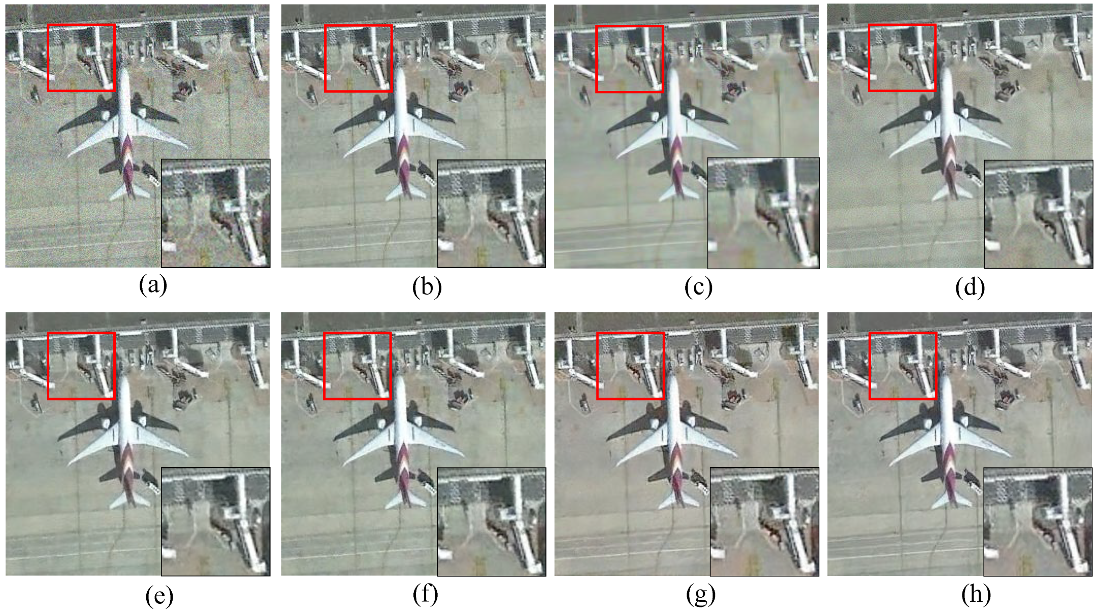
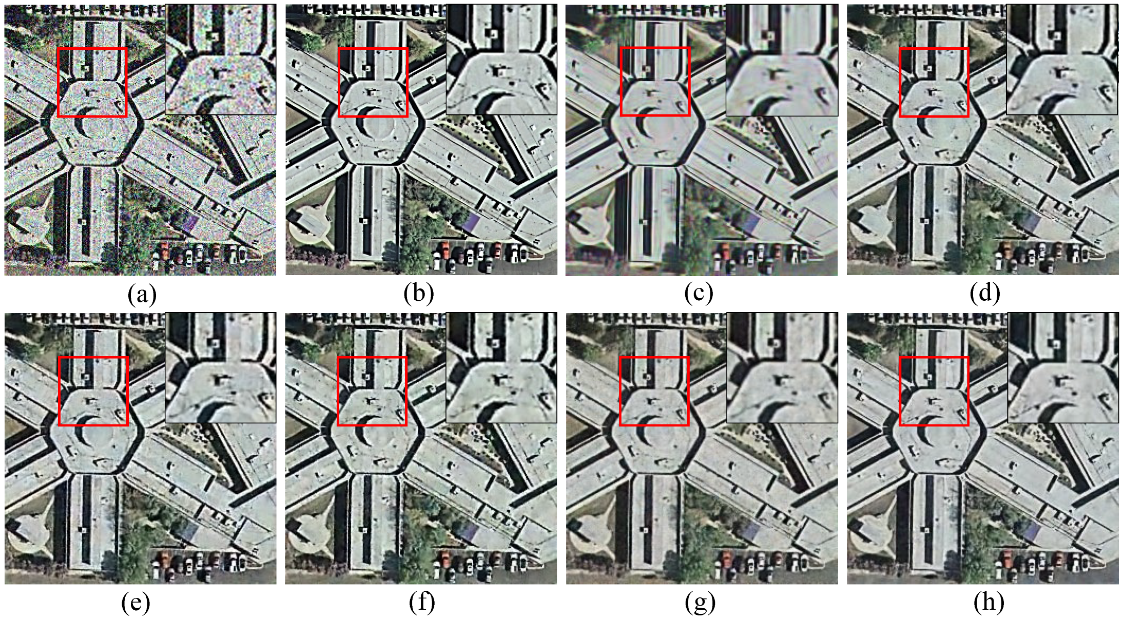
The performance of each method in NWPU-RESISC45 dataset is shown in Figure 7 and Figure 8. Figure 7 shows the effect of each method with the addition of AWGN with σ = 15. It can be seen that when the noise is weak, all methods except BM3D can restore the image details better. However, from the area with simple texture such as airport runway, we can see that FICL method has better noise suppression and purer image.
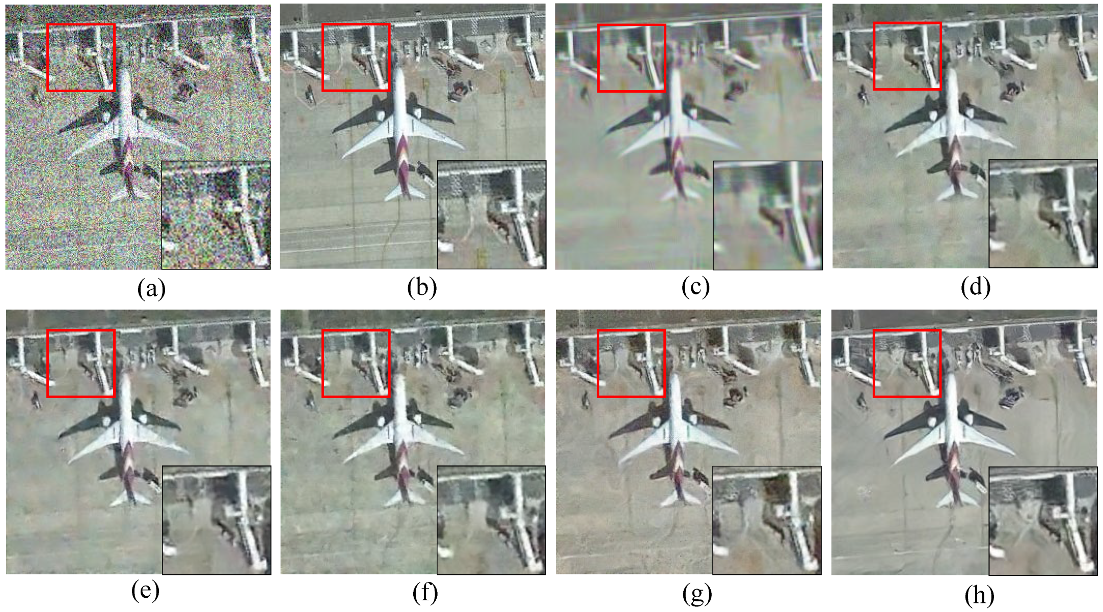
Figure 8 shows the effect of each method with the addition of AWGN with σ = 50. It can be seen that the scene of high-intensity noise has brought great challenges to various methods. DnCNN performs poorly in noise suppression and texture detail restoration. DUMNR has a certain ability to suppress noise, but the restored image quality is not good enough. CBDNet appeared obvious smear marks in high noise scenes. The ability of DGCL to restore detail texture is still insufficient. The proposed FICL method can restore the image texture details more effectively than other methods on the basis of effectively suppressing noise.
The performance of each method in UCMerced_LandUse dataset is shown in Figure 9 and Figure 10. Similarly, we add AWGN with σ = 15 and σ = 50 in Figure 8 and Figure 9. The results are similar to the display effect of the NWPU-RESISC45 dataset. Our FICL method has advantages over other methods in both noise removal and texture detail recovery. This shows that FICL method not only has excellent performance, but also has good versatility.
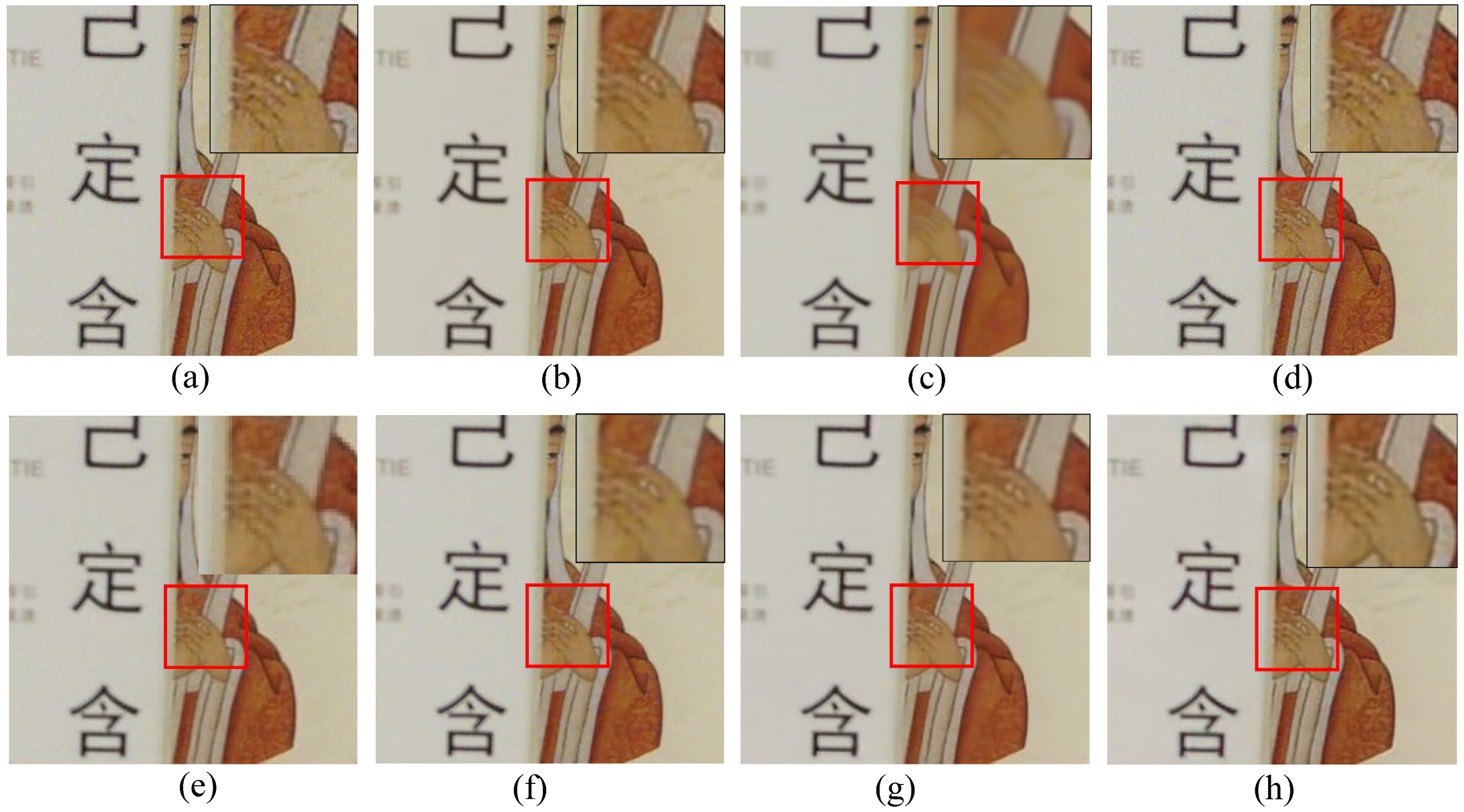
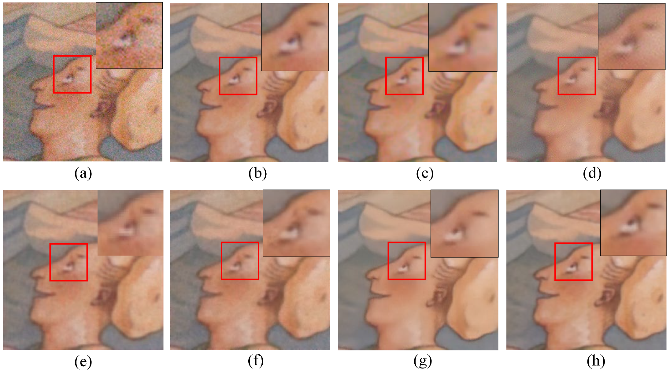
Figure 11, Figure 12, Figure 13 and Figure 14 visually demonstrate the quality of the images reconstructed by each method on the PolyU and SIDD datasets. Upon examination, it becomes evident that BM3D’s denoised outputs exhibit excessive smoothing, leading to a loss of fine details. Conversely, DnCNN’s results struggle to effectively eliminate real-world noise. DUMRN demonstrates commendable noise suppression, yet the restored images retain noticeable graininess. CBDNet achieves significant noise reduction but at the cost of introducing smear-like artifacts that impair image clarity. Both DGCL and FICL, grounded in complementary learning, exhibit distinct characteristics. While DGCL prioritizes noise suppression while preserving some image texture details, the quality of the restored images falls short of that achieved by FICL. As a result, FICL’s denoised images appear purer and richer in detail, striking a balance between noise removal and texture preservation.

3.3.3. Effect in Application Scenarios

To investigate the impact of our denoising method on downstream tasks, we used AlexNet to perform image classification on the UCMerced LandUse dataset in noise free, noisy, and denoising scenarios. Table 5 shows the classification accuracy of AlexNet under different scenarios.
As shown in Table 5, Alexnet achieves the highest accuracy in a noiseless scenario (σ = 0). Alexnet still achieves the highest classification accuracy in a weak noise scenario with the addition of AWGN σ = 10. When AWGN’s σ is greater than or equal to 20, Alexnet’s classification accuracy begins to suffer. Before using Alexnet to classify images, we used FICL to denoise images containing AWGN with σ greater than or equal to 20. The accuracy of classification of denoised images is significantly improved. The image containing AWGN with σ = 50 can decrease the AlexNet image classification accuracy by 0.222, but after denoising the AlexNet image classification accuracy only decreases by 0.0645. This shows that our proposed FICL method can effectively reduce the impact of noise on the downstream task.

4. Discussion

We performed ablation studies to highlight the significance of the various components within our FICL framework. We tested the case of only NP, RIP, and the fusion of those results without an FIM module. From Table 6 and Table 7, it can be seen that NP has advantages in low-noise scenarios, but its performance decreases significantly with increasing noise intensity. RIP performs worse than RP in low-noise environments, but its performance is relatively stable, and the quality of the generated images does not significantly decrease with increasing noise intensity. The fusion result generated by complementary learning of NP and RIP can combine the advantages of both and improve the denoising effect. The FIM can further enhance the denoising effect. In the experiment of the real-world denoising datasets, Table 8 shows that the effect of the FIM is more significant.

5. Conclusions

In this work, we propose an effective image denoising model, termed the FICL model, which is mainly composed of NP, RIP, FIM, and a fusion module. The FICL model not only realizes the fusion of denoising results in complementary learning, but also realizes the interaction of features in NP and RIP networks, which is a deeper complementary learning. The FICL model is validated on two remote sensing datasets (NWPU-RESISC45 and UCMerced_LandUse) and two real-word denoising datasets (PolyU and SIDD). The findings reveal that, compared with other methods listed in the paper, FICL has better performance in PSNR and SSIM evaluation indexes. The image processing based on FICL network also has good visual effect, especially in high noise scenes, it can effectively remove noise and restore texture details. Finally, the ablation experiment proves the effectiveness of each part of the FICL network, especially the FIM has a significant role in improving the network performance. In a word, the proposed FICL model has a good application prospect in actual image denoising.

Author Contributions

S.Z., Y.D., H.W. and M.Z. provided the ideas; S.Z. and X.C. implemented this algorithm; S.Z. wrote this paper; H.W., Y.D., Y.H. and M.Z. revised this paper. All authors have read and agreed to the published version of the manuscript.

Funding

This research was funded by the Fundamental Research Funds for the Central Universities, and the Innovation Fund of Xidian University (No: YJSJ24019).

Data Availability Statement

The public datasets are used in this study, no new data are created or analyzed. Data sharing is not applicable to this article.

Acknowledgments

We thank the authors who provided experimental datasets and compared methods.

Conflicts of Interest

The authors declare no conflicts of interest.

References

  1. Feng, X.; Zhang, W.; Su, X.; Xu, Z. Optical Remote Sensing Image Denoising and Super-Resolution Reconstructing Using Optimized Generative Network in Wavelet Transform Domain. Remote Sens. 2021, 13, 1858. [Google Scholar] [CrossRef]
  2. Qi, J.; Wan, P.; Gong, Z.; Xue, W.; Yao, A.; Liu, X.; Zhong, P. A Self-Improving Framework for Joint Depth Estimation and Underwater Target Detection from Hyperspectral Imagery. Remote Sens. 2021, 13, 1721. [Google Scholar] [CrossRef]
  3. Zhu, Y.; Yang, G.; Yang, H.; Zhao, F.; Han, S.; Chen, R.; Zhang, C.; Yang, X.; Liu, M.; Cheng, J.; et al. Estimation of Apple Flowering Frost Loss for Fruit Yield Based on Gridded Meteorological and Remote Sensing Data in Luochuan, Shaanxi Province, China. Remote Sens. 2021, 13, 1630. [Google Scholar] [CrossRef]
  4. Zhang, J.; Zhang, X.; Tang, X.; Huang, Z.; Jiao, L. Vehicle Detection and Tracking in Remote Sensing Satellite Vidio Based on Dynamic Association. In Proceedings of the 2019 10th International Workshop on the Analysis of Multitemporal Remote Sensing Images (Multitemp), Shanghai, China, 5–7 August 2019. [Google Scholar]
  5. Xia, J.; Wang, Y.; Zhou, M.; Deng, S.; Wang, Z. Variations in Channel Centerline Migration Rate and Intensity of a Braided Reach in the Lower Yellow River. Remote Sens. 2021, 13, 1680. [Google Scholar] [CrossRef]
  6. Lin, S.; Zhang, M.; Cheng, X.; Shi, L.; Gamba, P.; Wang, H. Dynamic Low-Rank and Sparse Priors Constrained Deep Autoencoders for Hyperspectral Anomaly Detection. IEEE Trans. Instrum. Meas. 2024, 73, 2500518. [Google Scholar] [CrossRef]
  7. Cheng, X.; Huo, Y.; Lin, S.; Dong, Y.; Zhao, S.; Zhang, M.; Wang, H. Deep Feature Aggregation Network for Hyperspectral Anomaly Detection. IEEE Trans. Instrum. Meas. 2024, 73, 5033016. [Google Scholar] [CrossRef]
  8. Yuan, Q.; Zhang, Q.; Li, J.; Shen, H.; Zhang, L. Hyperspectral Image Denoising Employing a Spatial-Spectral Deep Residual Convolutional Neural Network. IEEE Trans. Geosci. Remote Sens. 2019, 57, 1205–1218. [Google Scholar] [CrossRef]
  9. Dabov, K.; Foi, A.; Katkovnik, V.; Egiazarian, K. Image Denoising by Sparse 3-D Transform-Domain Collaborative Filtering. IEEE Trans. Image Process. 2007, 16, 2080–2095. [Google Scholar] [CrossRef]
  10. Gu, S.; Zhang, L.; Zuo, W.; Feng, X. Weighted Nuclear Norm Minimization with Application to Image Denoising. In Proceedings of the 2014 IEEE Conference on Computer Vision and Pattern Recognition, Columbus, OH, USA, 23–28 June 2014; pp. 2862–2869. [Google Scholar]
  11. Xu, J.; Osher, S. Iterative Regularization and Nonlinear Inverse Scale Space Applied to Wavelet-Based Denoising. IEEE Trans. Image Process. 2007, 16, 534–544. [Google Scholar] [CrossRef]
  12. Roth, S.; Black, M.J. Fields of Experts. Int. J. Comput. Vis. 2009, 82, 205–229. [Google Scholar] [CrossRef]
  13. Anwar, S.; Porikli, F.; Huynh, C.P. Category-Specific Object Image Denoising. IEEE Trans. Image Process. 2017, 26, 5506–5518. [Google Scholar] [CrossRef] [PubMed]
  14. Luo, E.; Chan, S.H.; Nguyen, T.Q. Adaptive Image Denoising by Targeted Databases. IEEE Trans. Image Process. 2015, 24, 2167–2181. [Google Scholar] [CrossRef] [PubMed]
  15. He, W.; Yao, Q.; Li, C.; Yokoya, N.; Zhao, Q. Non-Local Meets Global: An Integrated Paradigm for Hyperspectral Denoising. In Proceedings of the 2019 IEEE/CVF Conference on Computer Vision and Pattern Recognition (CVPR 2019), Long Beach, CA, USA, 15–20 June 2019; pp. 6861–6870. [Google Scholar]
  16. Kong, X.; Zhao, Y.; Chan, J.C.-W.; Xue, J. Hyperspectral Image Restoration via Spatial-Spectral Residual Total Variation Regularized Low-Rank Tensor Decomposition. Remote Sens. 2022, 14, 511. [Google Scholar] [CrossRef]
  17. Xu, S.; Cao, X.; Peng, J.; Ke, Q.; Ma, C.; Meng, D. Hyperspectral Image Denoising by Asymmetric Noise Modeling. IEEE Trans. Geosci. Remote Sens. 2022, 60, 5545214. [Google Scholar] [CrossRef]
  18. Liu, J.; Li, J.; Liu, T.; Tam, J. Graded Image Generation Using Stratified CycleGAN. Med. Image Comput. Comput. Assist. Interv. 2020, 12262, 760–769. [Google Scholar] [CrossRef] [PubMed]
  19. Lyu, Q.; Guo, M.; Ma, M. Boosting Attention Fusion Generative Adversarial Network for Image Denoising. Neural Comput. Appl. 2021, 33, 4833–4847. [Google Scholar] [CrossRef]
  20. Cheng, X.; Zhang, M.; Lin, S.; Li, Y.; Wang, H. Deep Self-Representation Learning Framework for Hyperspectral Anomaly Detection. IEEE Trans. Instrum. Meas. 2024, 73, 5002016. [Google Scholar] [CrossRef]
  21. Huo, Y.; Qian, X.; Li, C.; Wang, W. Multiple Instance Complementary Detection and Difficulty Evaluation for Weakly Supervised Object Detection in Remote Sensing Images. IEEE Geosci. Remote Sens. Lett. 2023, 20, 6006505. [Google Scholar] [CrossRef]
  22. Zhou, K.; Zhang, M.; Wang, H.; Tan, J. Ship Detection in SAR Images Based on Multi-Scale Feature Extraction and Adaptive Feature Fusion. Remote Sens. 2022, 14, 755. [Google Scholar] [CrossRef]
  23. Lin, S.; Zhang, M.; Cheng, X.; Zhou, K.; Zhao, S.; Wang, H. Dual Collaborative Constraints Regularized Low-Rank and Sparse Representation via Robust Dictionaries Construction for Hyperspectral Anomaly Detection. IEEE J. Sel. Top. Appl. Earth Obs. Remote Sens. 2023, 16, 2009–2024. [Google Scholar] [CrossRef]
  24. Lin, S.; Zhang, M.; Cheng, X.; Zhou, K.; Zhao, S.; Wang, H. Hyperspectral Anomaly Detection via Sparse Representation and Collaborative Representation. IEEE J. Sel. Top. Appl. Earth Observ. Remote Sens. 2023, 16, 946–961. [Google Scholar] [CrossRef]
  25. Huo, Y.; Cheng, X.; Lin, S.; Zhang, M.; Wang, H. Memory-Augmented Autoencoder with Adaptive Reconstruction and Sample Attribution Mining for Hyperspectral Anomaly Detection. IEEE Trans. Geosci. Remote Sens. 2024, 62, 5518118. [Google Scholar] [CrossRef]
  26. Lin, S.; Cheng, X.; Zeng, Y.; Huo, Y.; Zhang, M.; Wang, H. Low-Rank and Sparse Representation Inspired Interpretable Network for Hyperspectral Anomaly Detection. IEEE Trans. Instrum. Meas. 2024, 73, 5033116. [Google Scholar] [CrossRef]
  27. Cheng, X.; Zhang, M.; Lin, S.; Zhou, K.; Zhao, S.; Wang, H. Two-Stream Isolation Forest Based on Deep Features for Hyperspectral Anomaly Detection. IEEE Geosci. Remote Sens. Lett. 2023, 20, 5504205. [Google Scholar] [CrossRef]
  28. Zhang, K.; Zuo, W.; Chen, Y.; Meng, D.; Zhang, L. Beyond a Gaussian Denoiser: Residual Learning of Deep CNN for Image Denoising. IEEE Trans. Image Process. 2017, 26, 3142–3155. [Google Scholar] [CrossRef]
  29. Zhang, K.; Zuo, W.; Zhang, L. FFDNet: Toward a Fast and Flexible Solution for CNN-Based Image Denoising. IEEE Trans. Image Process. 2018, 27, 4608–4622. [Google Scholar] [CrossRef]
  30. Guo, S.; Yan, Z.; Zhang, K.; Zuo, W.; Zhang, L. Toward Convolutional Blind Denoising of Real Photographs. In Proceedings of the 2019 IEEE/CVF Conference on Computer Vision and Pattern Recognition (CVPR), Long Beach, CA, USA, 15–20 June 2019; pp. 1712–1722. [Google Scholar]
  31. Anwar, S.; Barnes, N. Real Image Denoising with Feature Attention. In Proceedings of the 2019 IEEE/CVF International Conference on Computer Vision (ICCV), Seoul, Republic of Korea, 27 October–2 November 2019; pp. 3155–3164. [Google Scholar]
  32. Chang, M.; Li, Q.; Feng, H.; Xu, Z. Spatial-Adaptive Network for Single Image Denoising. In Proceedings of the Computer Vision—ECCV 2020; Vedaldi, A., Bischof, H., Brox, T., Frahm, J.-M., Eds.; Springer International Publishing: Cham, Switzerland, 2020; pp. 171–187. [Google Scholar]
  33. Han, L.; Zhao, Y.; Lv, H.; Zhang, Y.; Liu, H.; Bi, G. Remote Sensing Image Denoising Based on Deep and Shallow Feature Fusion and Attention Mechanism. Remote Sens. 2022, 14, 1243. [Google Scholar] [CrossRef]
  34. Xu, J.; Yuan, M.; Yan, D.-M.; Wu, T. Deep Unfolding Multi-Scale Regularizer Network for Image Denoising. Comput. Vis. Media 2023, 9, 335–350. [Google Scholar] [CrossRef]
  35. Li, J.; Wang, J.; Lin, F.; Wu, W.; Chen, Z.-M.; Heidari, A.A.; Chen, H. DSEUNet: A Lightweight UNet for Dynamic Space Grouping Enhancement for Skin Lesion Segmentation. Expert Syst. Appl. 2024, 255, 124544. [Google Scholar] [CrossRef]
  36. Wu, Y.; Zhang, J.; Liu, D. A Remote Sensing Hyperspectral Image Noise Removal Method Based on Multipriors Guidance. IEEE Geosci. Remote Sens. Lett. 2024, 21, 5504805. [Google Scholar] [CrossRef]
  37. Goodfellow, I.; Pouget-Abadie, J.; Mirza, M.; Xu, B.; Warde-Farley, D.; Ozair, S.; Courville, A.; Bengio, Y. Generative Adversarial Networks. Commun. ACM 2020, 63, 139–144. [Google Scholar] [CrossRef]
  38. Zhu, M.-L.; Zhao, L.-L.; Xiao, L. Image Denoising Based on GAN with Optimization Algorithm. Electronics 2022, 11, 2445. [Google Scholar] [CrossRef]
  39. Chen, S.; Shi, D.; Sadiq, M.; Cheng, X. Image Denoising with Generative Adversarial Networks and Its Application to Cell Image Enhancement. IEEE Access 2020, 8, 82819–82831. [Google Scholar] [CrossRef]
  40. Lyu, Q.; Guo, M.; Pei, Z. DeGAN: Mixed Noise Removal via Generative Adversarial Networks. Appl. Soft. Comput. 2020, 95, 106478. [Google Scholar] [CrossRef]
  41. Wang, Y.; Chang, D.; Zhao, Y. A New Blind Image Denoising Method Based on Asymmetric Generative Adversarial Network. IET Image Process. 2021, 15, 1260–1272. [Google Scholar] [CrossRef]
  42. Pan, S.; Ma, J.; Fu, X.; Chen, D.; Xu, N.; Qin, G. Denoising Research of Petrographic Thin Section Images with the Global Residual Generative Adversarial Network. Geoenergy Sci. Eng. 2023, 220, 111204. [Google Scholar] [CrossRef]
  43. Huang, Y.; Xia, W.; Lu, Z.; Liu, Y.; Chen, H.; Zhou, J.; Fang, L.; Zhang, Y. Noise-Powered Disentangled Representation for Unsupervised Speckle Reduction of Optical Coherence Tomography Images. IEEE Trans. Med. Imaging 2021, 40, 2600–2614. [Google Scholar] [CrossRef] [PubMed]
  44. Han, Z.; Hong, S.; Xiong, Z.; Cui, X.; Yue, W. A Coarse-to-Fine Multi-Scale Feature Hybrid Low-Dose CT Denoising Network. Signal Process.-Image Commun. 2023, 118, 117009. [Google Scholar] [CrossRef]
  45. Zheng, Y.; Su, J.; Zhang, S.; Tao, M.; Wang, L. Dehaze-AGGAN: Unpaired Remote Sensing Image Dehazing Using Enhanced Attention-Guide Generative Adversarial Networks. IEEE Trans. Geosci. Remote Sens. 2022, 60, 1–13. [Google Scholar] [CrossRef]
  46. Chen, X.; Huang, Y. Memory-Oriented Unpaired Learning for Single Remote Sensing Image Dehazing. IEEE Geosci. Remote Sens. Lett. 2022, 19, 3511705. [Google Scholar] [CrossRef]
  47. Jin, M.; Wang, P.; Li, Y. HyA-GAN: Remote Sensing Image Cloud Removal Based on Hybrid Attention Generation Adversarial Network. Int. J. Remote Sens. 2024, 45, 1755–1773. [Google Scholar] [CrossRef]
  48. Kas, M.; Chahi, A.; Kajo, I.; Ruichek, Y. DLL-GAN: Degradation-Level-Based Learnable Adversarial Loss for Image Enhancement. Expert Syst. Appl. 2024, 237, 121666. [Google Scholar] [CrossRef]
  49. Geng, M.; Meng, X.; Yu, J.; Zhu, L.; Jin, L.; Jiang, Z.; Qiu, B.; Li, H.; Kong, H.; Yuan, J.; et al. Content-Noise Complementary Learning for Medical Image Denoising. IEEE Trans. Med. Imaging 2022, 41, 407–419. [Google Scholar] [CrossRef] [PubMed]
  50. Zhao, S.; Lin, S.; Cheng, X.; Zhou, K.; Zhang, M.; Wang, H. Dual-GAN Complementary Learning for Real-World Image Denoising. IEEE Sens. J. 2024, 24, 355–366. [Google Scholar] [CrossRef]
  51. Lu, W.; Onofrey, J.A.; Lu, Y.; Shi, L.; Ma, T.; Liu, Y.; Liu, C. An Investigation of Quantitative Accuracy for Deep Learning Based Denoising in Oncological PET. Phys. Med. Biol. 2019, 64, 165019. [Google Scholar] [CrossRef] [PubMed]
  52. Chen, H.; Zhang, Y.; Kalra, M.K.; Lin, F.; Chen, Y.; Liao, P.; Zhou, J.; Wang, G. Low-Dose CT with a Residual Encoder-Decoder Convolutional Neural Network. IEEE Trans. Med. Imaging 2017, 36, 2524–2535. [Google Scholar] [CrossRef]
  53. Gao, S.-H.; Cheng, M.-M.; Zhao, K.; Zhang, X.-Y.; Yang, M.-H.; Torr, P. Res2Net: A New Multi-Scale Backbone Architecture. IEEE Trans. Pattern Anal. Mach. Intell. 2021, 43, 652–662. [Google Scholar] [CrossRef] [PubMed]
  54. He, K.; Zhang, X.; Ren, S.; Sun, J. Deep Residual Learning for Image Recognition. In Proceedings of the 2016 IEEE Conference on Computer Vision and Pattern Recognition (CVPR), Las Vegas, NV, USA, 27–30 June 2016; pp. 770–778. [Google Scholar]
  55. Ronneberger, O.; Fischer, P.; Brox, T. U-Net: Convolutional Networks for Biomedical Image Segmentation. In Proceedings of the Medical Image Computing and Computer-Assisted Intervention—MICCAI 2015; Navab, N., Hornegger, J., Wells, W.M., Frangi, A.F., Eds.; Springer International Publishing: Cham, Switzerland, 2015; pp. 234–241. [Google Scholar]
  56. Woo, S.; Park, J.; Lee, J.-Y.; Kweon, I.S. CBAM: Convolutional Block Attention Module. In Proceedings of the Computer Vision—ECCV 2018; Ferrari, V., Hebert, M., Sminchisescu, C., Weiss, Y., Eds.; Springer International Publishing: Cham, Switzerland, 2018; pp. 3–19. [Google Scholar]
  57. Lai, W.S.; Huang, J.B.; Ahuja, N.; Yang, M.H. Deep Laplacian Pyramid Networks for Fast and Accurate Super-Resolution. In Proceedings of the IEEE Conference on Computer Vision & Pattern Recognition, Honolulu, HI, USA, 21–26 July 2017; pp. 5835–5843. [Google Scholar]
  58. Wang, Z.; Bovik, A.C.; Sheikh, H.R.; Simoncelli, E.P. Image Quality Assessment: From Error Visibility to Structural Similarity. IEEE Trans. Image Process. 2004, 13, 600–612. [Google Scholar] [CrossRef]
  59. Jiang, K.; Wang, Z.; Yi, P.; Chen, C.; Huang, B.; Luo, Y.; Ma, J.; Jiang, J. Multi-Scale Progressive Fusion Network for Single Image Deraining. In Proceedings of the 2020 IEEE/CVF Conference on Computer Vision and Pattern Recognition (CVPR), Seattle, WA, USA, 13–19 June 2020. [Google Scholar] [CrossRef]
  60. Kamgar-Parsi, B.; Kamgar-Parsi, B. Optimally Isotropic Laplacian Operator. IEEE Trans. Image Process. 1999, 8, 1467–1472. [Google Scholar] [CrossRef]
  61. Cheng, G.; Han, J.; Lu, X. Remote Sensing Image Scene Classification: Benchmark and State of the Art. Proc. IEEE 2017, 105, 1865–1883. [Google Scholar] [CrossRef]
  62. Yang, Y.; Newsam, S. Bag-of-Visual-Words and Spatial Extensions for Land-Use Classification. In Proceedings of the 18th SIGSPATIAL International Conference on Advances in Geographic Information Systems, San Jose, CA, USA, 3–5 November 2010; pp. 270–279. [Google Scholar] [CrossRef]
  63. Xu, J.; Li, H.; Liang, Z.; Zhang, D.; Zhang, L. Real-World Noisy Image Denoising: A New Benchmark. arXiv 2018. [Google Scholar] [CrossRef]
  64. Plotz, T.; Roth, S. Benchmarking Denoising Algorithms with Real Photographs. In Proceedings of the 2017 IEEE Conference on Computer Vision and Pattern Recognition (CVPR), Honolulu, HI, USA, 21–26 July 2017; IEEE: Honolulu, HI, USA, 2017; pp. 2750–2759. [Google Scholar]
  65. Huynh-Thu, Q.; Ghanbari, M. Scope of Validity of PSNR in Image/Video Quality Assessment. Electron. Lett. 2008, 44, 800. [Google Scholar] [CrossRef]
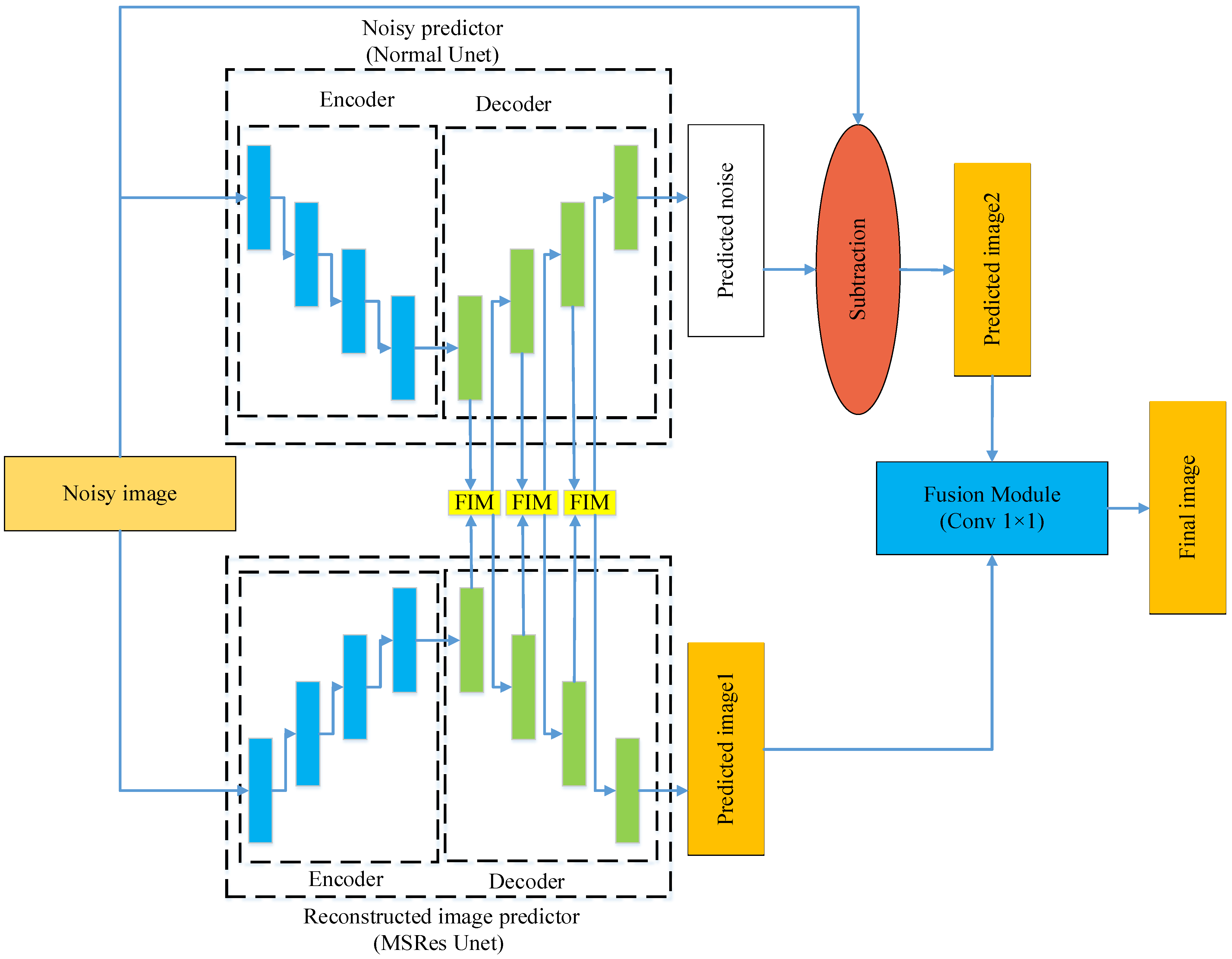
Figure 1. Structure diagram of feature interactive complementary learning (FICL) remote sensing image denoising strategy.
Remotesensing 16 03820 g001
Figure 2. (a) Res2Net module and (b) MSResNet module.
Remotesensing 16 03820 g002
Figure 3. RIP structure diagram based on multi-scale ResNet (MSResNet). MSResUnet adopts the unset structure improved by CBAM and MSResNet. The k, n, and s represent kernel size, channel number, and step of each cycle layer, respectively.
Remotesensing 16 03820 g003
Figure 4. Structure diagram of noise predictor (NP) based on Unet. The k, n, and s represent kernel size, channel number, and step of each convolution layer and deconvolution layer, respectively.
Remotesensing 16 03820 g004
Figure 5. Structure diagram of FIM.
Remotesensing 16 03820 g005
Figure 6. Structure diagram of fusion module.
Remotesensing 16 03820 g006
Figure 7. The figure shows the visual comparison of denoising performance of various methods on NWPU-RESISC45 dataset when the noise level σ = 15. (a) Noisy image. (b) Clean image. (c) BM3D. (d) DnCNN. (e) DUMNP. (f) CBDNet. (g) DGCL. (h) FICL. The red box marks the magnified area.
Remotesensing 16 03820 g007
Figure 8. The figure shows the visual comparison of denoising performance of various methods on NWPU-RESISC45 data set when the noise level σ = 50. (a) Noisy image. (b) Clean image. (c) BM3D. (d) DnCNN. (e) DUMNP. (f) CBDNet. (g) DGCL. (h) FICL. The red box marks the magnified area.
Remotesensing 16 03820 g008
Figure 9. The figure shows the visual comparison of the denoising performance of various methods on the UCMerced_LandUse dataset when the noise level σ = 15. (a) Noisy image. (b) Clean image. (c) BM3D. (d) DnCNN. (e) DUMNP. (f) CBDNet. (g) DGCL. (h) FICL. The red box marks the magnified area.
Remotesensing 16 03820 g009
Figure 10. The figure shows the visual comparison of the denoising performance of various methods on the UCMerced_LandUse dataset when the noise level σ = 50. (a) Noisy image. (b) Clean image. (c) BM3D. (d) DnCNN. (e) DUMNP. (f) CBDNet. (g) DGCL. (h) FICL. The red box marks the magnified area.
Remotesensing 16 03820 g010
Figure 11. The visual demonstration showcasing the effectiveness of diverse denoising methodologies applied to example 1 of the PolyU dataset is presented. (a) Noisy image. (b) Clean image. (c) BM3D. (d) DnCNN. (e) DUMNP. (f) CBDNet. (g) DGCL. (h) FICL. The red box marks the magnified area.
Remotesensing 16 03820 g011
Figure 12. The visual demonstration showcasing the effectiveness of diverse denoising methodologies applied to example 2 of the PolyU dataset is presented. (a) Noisy image. (b) Clean image. (c) BM3D. (d) DnCNN. (e) DUMNP. (f) CBDNet. (g) DGCL. (h) FICL. The red box marks the magnified area.
Remotesensing 16 03820 g012
Figure 13. The visual demonstration showcasing the effectiveness of diverse denoising methodologies applied to example 1 of the SIDD dataset is presented. (a) Noisy image. (b) Clean image. (c) BM3D. (d) DnCNN. (e) DUMNP. (f) CBDNet. (g) DGCL. (h) FICL. The red box marks the magnified area.
Remotesensing 16 03820 g013
Figure 14. The visual demonstration showcasing the effectiveness of diverse denoising methodologies applied to example 2 of the SIDD dataset is presented. (a) Noisy image. (b) Clean image. (c) BM3D. (d) DnCNN. (e) DUMNP. (f) CBDNet. (g) DGCL. (h) FICL. The red box marks the magnified area.
Remotesensing 16 03820 g014
Table 1. The evaluation metrics of different methods in the NWPU-RESISC45 dataset. The average PSNR (dB)/SSIM is utilized to measure the denoising performance in the table, and the bold font indicates the best effect. The bold font indicates the best effect.
KERRYPNXσ = 5σ = 10σ = 20σ = 30σ = 40σ = 50
BM3D37.46/0.958633.19/0.912129.35/0.832327.44/0.768526.04/0.719125.18/0.6826
DnCNN38.99/0.969635.10/0.930031.39/0.860329.60/0.811828.36/0.772927.33/0.7355
DUMRN36.34/0.965234.47/0.942331.65/0.889029.82/0.839428.51/0.793327.47/0.7523
CBDNet39.08/0.975735.35/0.945031.73/0.888729.69/0.834828.26/0.784727.15/0.7383
DGCL35.48/0.960233.60/0.932930.72/0.868729.12/0.819127.91/0.772026.88/0.7238
FICL (ours)39.14/0.979935.99/0.957032.48/0.907530.54/0.863529.23/0.825228.24/0.7913
Table 2. The evaluation metrics of different methods in the UCMerced_LandUse dataset. The average PSNR (dB)/SSIM is utilized to measure the denoising performance in the table, and the bold font indicates the best effect. The bold font indicates the best effect.
σ = 5σ = 10σ = 20σ = 30σ = 40σ = 50
BM3D36.27/0.965932.17/0.921828.43/0.873825.83/0.841122.57/0.809420.12/0.7719
DnCNN35.67/0.946732.77/0.899329.82/0.830228.39/0.794227.32/0.764526.46/0.7409
DUMRN33.53/0.943732.38/0.924030.31/0.879128.79/0.838027.58/0.799226.58/0.7633
CBDNet36.21/0.952333.19/0.924030.41/0.880728.78/0.833727.47/0.793426.40/0.7523
DGCL32.64/0.929531.41/0.904229.42/0.852728.11/0.813927.05/0.775426.08/0.7342
FICL(ours)36.34/0.949233.26/0.927930.87/0.885229.35/0.849928.23/0.819227.34/0.7912
Table 3. The average PSNR (dB) and SSIM of the various methods are presented herewith, in the PolyU test dataset. The bold font indicates the best effect.
PSNRSSIM
BM3D33.510.9027
DnCNN33.970.9142
DUMRN37.450.9489
CBDNet37.860.9621
DGCL38.110.9613
FICL (ours)38.410.9652
Table 4. The average PSNR (dB) and SSIM of the various methods are presented herewith, in the SIDD test dataset. The bold font indicates the best effect.
PSNRSSIM
BM3D33.900.8915
DnCNN32.590.8764
DUMRN36.750.9032
CBDNet36.630.9085
DGCL37.330.9133
FICL (ours)37.450.9146
Table 5. The image classification accuracy of AlexNet on the UCMerced LandUse dataset in noise free, noisy, and denoised scenarios. The bold font indicates the best effect.
σ = 0σ = 10σ = 20σ = 30σ = 40σ = 50
Accuracy with noisy0.76370.76370.72550.69450.63240.5417
Accuracy with denoising0.76130.73030.71830.6992
Table 6. FICL component validity studies in NWPU-RESISC45 dataset. The average PSNR (dB)/SSIM is utilized to measure the denoising performance in the table, and the bold font indicates the best effect.
σ = 5σ = 10σ = 20σ = 30σ = 40σ = 50
Only NP38.02/0.974835.12/0.951431.91/0.896530.11/0.843928.57/0.786227.14/0.7174
Only RIP37.36/0.973634.99/0.950931.87/0.900730.03/0.855628.76/0.815927.80/0.7807
Fusion without FIM38.20/0.976635.45/0.954132.12/0.903630.23/0.858528.94/0.818827.95/0.7825
FICL (ours)39.14/0.979935.99/0.957032.48/0.907530.54/0.863529.23/0.825228.24/0.7913
Table 7. FICL component validity studies in UCMerced_LandUse dataset. The Average PSNR (dB)/SSIM is utilized to measure the denoising performance in the table, and the bold font indicates the best effect.
σ = 5σ = 10σ = 20σ = 30σ = 40σ = 50
Only NP34.36/0.944732.73/0.923230.48/0.876628.93/0.834127.60/0.787426.32/0.7287
Only RIP33.93/0.944032.56/0.922130.39/0.877828.91/0.841227.82/0.809626.94/0.7809
Fusion without FIM34.44/0.947332.92/0.925730.62/0.881929.11/0.845227.99/0.813327.09/0.7838
FICL (ours)36.34/0.949233.26/0.927930.87/0.885229.35/0.849928.23/0.819227.34/0.7912
Table 8. FICL component validity studies in PolyU and SIDD datasets. The Average PSNR (dB)/SSIM is utilized to measure the denoising performance in the table, and the bold font indicates the best effect.
Only NPOnly RIPFusion without FIMFICL
PolyU37.47/0.955836.94/0.951637.76/0.959638.41/0.9652
SIDD36.60/0.904236.21/0.902336.93/0.908737.45/0.9146
Disclaimer/Publisher’s Note: The statements, opinions and data contained in all publications are solely those of the individual author(s) and contributor(s) and not of MDPI and/or the editor(s). MDPI and/or the editor(s) disclaim responsibility for any injury to people or property resulting from any ideas, methods, instructions or products referred to in the content.