Predicting Rock Hardness and Abrasivity Using Hyperspectral Imaging Data and Random Forest Regressor Model

Abstract

This study aimed to develop predictive models for rock hardness and abrasivity based on hyperspectral imaging data, providing valuable information without interrupting the mining processes. The data collection stage first involved scanning 159 rock samples collected from 6 different blasted rock piles using visible and near-infrared (VNIR) and short-wave infrared (SWIR) sensors. The hardness and abrasivity of the samples were then determined through Leeb rebound hardness (LRH) and Cerchar abrasivity index (CAI) tests, respectively. The data preprocessing involved radiometric correction, background removal, and staking VNIR and SWIR images. An integrated approach based on K-means clustering and the band ratio concept was employed for feature extraction, resulting in 28 band-ratio-based features. Afterward, the random forest regressor (RFR) algorithm was employed to develop predictive models for rock hardness and abrasivity separately. The performance assessment showed that the developed models can estimate rock hardness and abrasivity of unseen data with R² scores of 0.74 and 0.79, respectively, with the most influential features located mainly within the SWIR region. The results indicate that integrated hyperspectral data and RFR technique have strong potential for practical and efficient rock hardness and abrasivity characterization during mining processes.

1. Introduction

The interaction between rocks and mechanical equipment is one of the most predominant phenomena in geoengineering projects, such as mining, milling, and rock excavation, and it can greatly affect the lifetime of mechanical tools [1,2]. This dynamic interaction between rocks and mechanical equipment significantly impacts mechanical equipment’s performance, efficiency, lifetime, and maintenance. A thorough understanding of this interaction is critically important for optimizing geoengineering operations [3]. Three distinct factors determine this interaction: the properties of rocks, the properties of mechanical tools, and how mechanical tools interact with rocks [4]. Regarding these three factors, only rock properties may vary significantly in different parts of a specific project, and the latter two terms are generally constants.

From a geomechanical point of view, rock hardness and abrasivity are among the most critical properties of rocks that determine how rocks interact with mechanical tools. Rock hardness generally refers to the rock’s ability to resist scratching, penetration, or permanent deformation [5]. Various testing methods have been developed to measure rock hardness, which can be categorized into four categories based on the mechanism they use: indentation, rebound, scratch, and grinding. A comprehensive review of the existing rock hardness testing methods and their advantages and limitations can be found in [6]. Among the mentioned categories, rebound tests are flexible, practical, nondestructive, and economically viable; therefore, they have been extensively applied in many geoengineering applications [7,8,9,10,11,12,13]. The rebound hardness category consists of a variety of testing methods, including Schmidt hammer (SH), Shore scleroscope, and Leeb rebound hardness (LRH), which are among the most commonly used ones [14]. In contrast, abrasion refers to the wearing or tearing away of particles from a solid surface [15]. Abrasion is a process that could cause the removal or displacement of material at a solid surface, leading to wear, especially on tools used in mining, drilling, milling, and tunneling applications. The Cerchar abrasivity index (CAI) is among the most widely used abrasion tests in geoengineering projects [16].

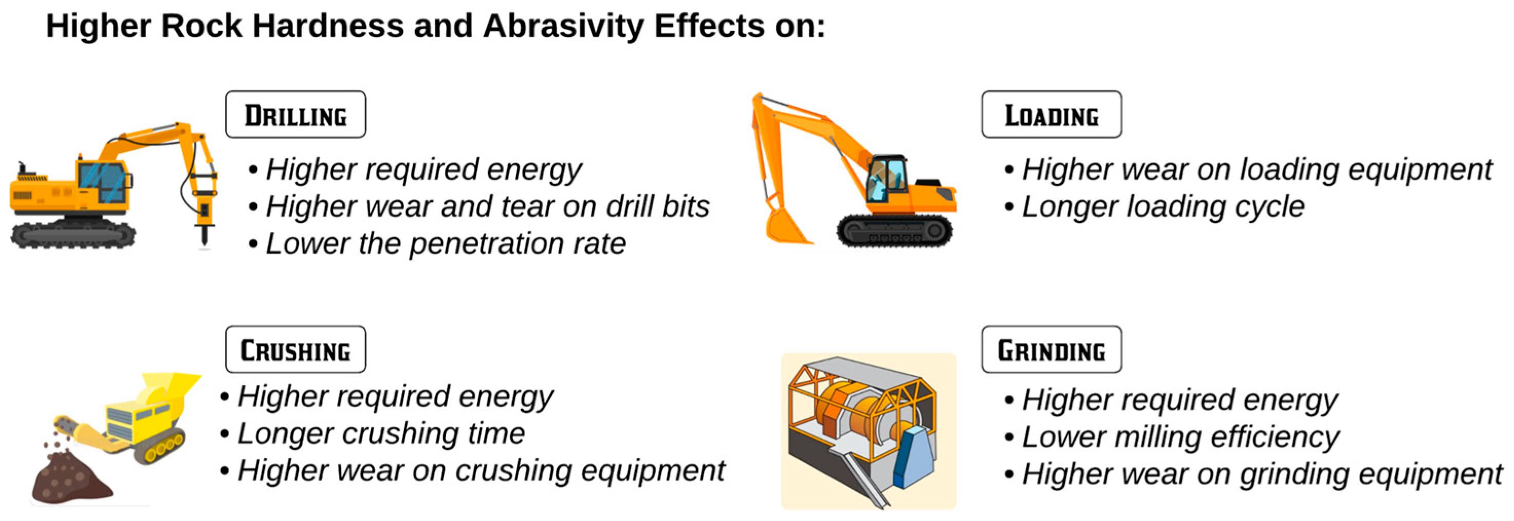
Rock hardness and abrasivity together could considerably affect all mining processes, from drilling to grinding. Figure 1 schematically illustrates how higher rock hardness and abrasivity could impact the entire mine-to-mill process. A brief description of the situation of facing high hardness and abrasive rock materials through each stage is provided here. In the drilling stage, the higher the hardness and abrasivity of the rocks, the higher the required energy for drilling, the lower the penetration rate, and the higher the wear and tear on drilling equipment (e.g., drill bit). Achieving acceptable fragmentation and blasting results (e.g., particle size distribution) requires more explosivity (higher blasting energy) in harder rocks than in softer ones. Increased wear and tear on the shovel bucket nails, loading cycling, and energy consumption are among the most adverse effects of hard rocks on shovels in the loading stage. Similar impacts can be seen in crushing and grinding. For example, feeding hard and more abrasive rock material into grinders for an extended period would decrease the efficiency of the comminution process, increase the comminution energy requirement, the wear of mill liners and ball consumption in ball mills, and increase the downtime for maintenance. More detailed information on the impacts of rock hardness and abrasivity on different mining and milling processes can be found in [6,17,18,19,20,21].

To date, numerous testing methods have been developed to assess rock hardness and abrasivity in the lab and on field scales. Like all other geomechanical testing methods, the proposed approaches for rock hardness and abrasivity have advantages and disadvantages [6]. On the one hand, these methods directly examine rock materials and provide engineers and decision-makers with insightful values. On the other hand, they are generally time-consuming, costly, and labor-demanding. To be more specific, these testing methods require rock samples to be collected, prepared, and tested, which in a mining operation environment simply means an interruption in the mining process, which is undesirable.

In this study, the primary focus is on the development of predictive models for rock hardness and abrasivity using remotely sensed hyperspectral imaging data. The aim is to provide decision-makers at mine sites with a nondestructive, contactless, and real-time method for estimating rock hardness and abrasivity. While previous research has explored the relationship between hyperspectral data and the mechanical properties of rocks, such as in references [22,23], these studies primarily utilized spectroradiometers for point measurements to investigate the correlation between rock properties and spectral information, which do not provide a sensing method. This study is one of the initial attempts to fill the gap in estimating rock hardness and abrasivity based on remotely sensed hyperspectral imaging data.

Hyperspectral imaging technology has emerged as a promising solution for automating the discrimination process in the past couple of decades. Hyperspectral imaging involves using an imaging spectrometer, also called a hyperspectral camera, to collect spectral information. A hyperspectral camera captures a scene’s light, separated into individual wavelengths or spectral bands. It provides a two-dimensional image of a scene while simultaneously recording the spectral information of each pixel in the image [24]. The rich spectral signatures obtained enable the differentiation of minerals based on their unique spectral patterns, i.e., absorption and reflectance. This capability paves the way for refined geological interpretations and resource assessments.

As a rapid, nondestructive, simultaneous multirange spectral technique, hyperspectral imaging can be applied in remote regions to rapidly collect a considerable amount of data, allowing engineers to better understand material characteristics throughout the entire mine-to-mill process. In the mining industry, hyperspectral remote sensing has been mainly used for mineral mapping, retrieving surface compositional information for mineral exploration, and for lithologic mapping and mine tailings with a focus on acid-generating minerals [25,26,27,28,29,30,31]. However, hyperspectral remote sensing has recently found its way into other geoengineering applications, such as characterizing rocks’ physical, geochemical, and mechanical properties [22,23,32,33,34,35,36,37,38,39].

Maras et al. [23] attempted to predict the physicomechanical properties of landscape rock samples using the mineralogical composition obtained as the arithmetic average of 16 spectroradiometer measurements. They claimed that although significant correlations were observed between the reflectance value of specific wavelengths and the physicomechanical properties of rocks, they could not confirm a cause-and-effect relationship, allowing them to predict the physicomechanical properties of rock through hyperspectral data. Schaefer et al. [32] explored the possibility of using reflectance spectroscopy to estimate the physical and mechanical properties of volcanic rocks, such as density, porosity, hardness, elasticity, and magnetic susceptibility. The authors assumed that these properties are related to the mineral composition and degradation of the rocks, which can be detected by the spectral signatures of iron-bearing minerals such as pyroxene, magnetite, and pyrite. The results of statistical analyses showed that reflectance spectroscopy has the potential to be a rapid and noninvasive method for characterizing volcanic rocks and suggested that aerial or satellite imaging spectroscopy could be used to map the geotechnical properties of volcanoes at a large scale. In similar studies, Kereszturi et al. [34] and Schaefer et al. [33] showed and confirmed the potential of hyperspectral imaging as a rapid and nondestructive method for characterizing the geomechanical properties of volcanic rocks. In another study by van Duijvenbode et al. [22] the use of material fingerprinting was discussed as a tool to investigate a link between rock hardness and rapidly acquired geochemical and hyperspectral data. The concept of material fingerprinting entails a fingerprint classification based on the similarity of the measured and constitutive material attributes. They concluded that the defined material fingerprints can explain material hardness, such as grindability. However, they did not propose a predictive model, and all conclusions were made based on visualization comparisons.

Considering that a mining project is an interconnected operation in which the performance of each stage impacts the performance of the downstream stages, the results of these predictive models could eventually help engineers and decision-makers better plan for the downstream processes. In fact, the hardness and abrasivity estimation from the hyperspectral scanning of a newly blasted rock pile could provide valuable information regarding the diggability, crushability, grindability of the materials, and their behavior during mining and processing in terms of ease and difficulty. For instance, knowing the hardness of ore rocks enables mineral processing engineers to make better decisions regarding the prioritizing of processing and mixing of different ore categories to reduce the milling time as the highest energy consumption sector in the entire mine-to-mill process. In addition, information obtained from the predictive models may also be used to optimize previous processes, such as drilling and blasting, by constantly updating and populating the mine database and block models, improving short-term mine planning. A good example of this situation could be using the obtained hardness and abrasivity information from each blasted rock pile to update and populate the geomechanical block model of the mine to better plan for future blast drillings.

2. Material and Methods

2.1. Framework of Study

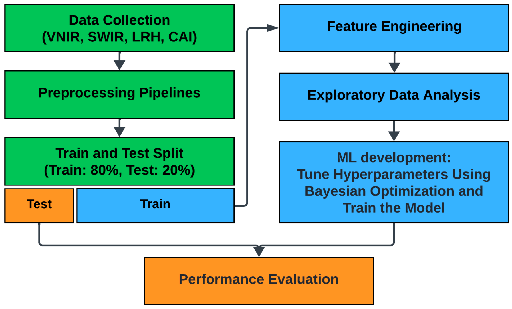
Figure 2 schematically illustrates the current research framework. The data collection comprises scanning rock samples using hyperspectral sensors and performing hardness and abrasivity tests on the collected rock samples. The preprocessing step mainly focuses on applying necessary filters on the hyperspectral data. Afterward, an appropriate train and test split is applied to the collected data, considering the distribution of rock hardness and abrasivity values. Next, a feature extraction approach based on K-means clustering and band ratio concept is developed to reduce the dimensionality of hyperspectral data. The last step deals with the development of predictive models and performance assessments. The specific approaches and methodologies applied in each step will be discussed in detail in the following.

2.2. Data Collection

A total of 159 handpicked rock samples were taken from 6 distinct blasted muck piles within a gold mine to cover all the rock types within the deposit. The collected rock samples mainly include sedimentary rocks with varying alteration degrees, mafic, ultramafic, and intrusive ones. To better understand the mineralogical composition of the studied area, 34 rock samples selected randomly from all six piles were sent for X-ray diffraction (XRD) analysis. The main reasons for sending only 34 rock samples are that not only is the XRD analysis a destructive, time- and cost-consuming process, but the rest of the rock samples are also required for other purposes. The obtained XRD results are provided in

Table 1. The results of XRD analysis on the selected 34 rock samples.

Sample	Q	B	M	Ch	D	Ca	P	T	M	H	A	Po
Pile1-01	13	1	0	0	0	6	3	0	0	0	47	30
Pile1-05	31	10	5	0	0	3	1	0	0	0	44	6
Pile1-10	19	16	12	1	0	1	1	0	0	0	38	12
Pile1-32	28	5	8	2	0	5	1	0	0	0	39	11
Pile1-48	20	1	2	1	0	7	4	0	0	0	22	43
Pile2-01	29	10	13	7	0	0	0	0	0	0	35	4
Pile2-02	31	9	24	5	0	0	0	0	0	0	28	2
Pile2-04	27	13	15	2	0	1	0	0	0	0	37	4
Pile2-08	18	16	1	2	0	0	1	0	0	0	55	5
Pile3-01	19	2	3	6	0	4	2	0	0	0	42	22
Pile3-02	0	0	0	23	6	7	0	51	3	9	1	0
Pile3-04	1	17	0	1	0	1	0	4	1	71	0	3
Pile3-06	0	0	0	24	5	3	0	59	4	3	1	0
Pile3-09	0	27	0	4	0	3	0	1	0	25	33	3
Pile3-12	24	2	4	0	0	0	0	0	0	0	64	5
Pile4-01	0	0	0	25	8	6	0	43	5	13	1	0
Pile4-03	0	35	0	2	0	5	0	2	0	7	39	4
Pile4-04	0	26	0	10	3	4	0	9	3	41	0	3
Pile4-05	13	3	4	0	0	3	0	0	0	0	72	5
Pile4-08	23	3	6	0	0	1	0	0	0	0	53	13
Pile4-10	10	3	3	0	0	3	1	0	0	0	70	8
Pile5-01	1	33	3	4	33	1	1	23	1	0	0	0
Pile5-02	30	12	13	3	0	0	0	0	0	0	37	4
Pile5-03	28	12	3	2	0	0	0	0	0	0	47	5
Pile5-04	0	1	0	24	10	0	0	11	6	48	0	0
Pile5-09	4	29	1	2	25	1	1	36	2	0	0	0
Pile5-10	2	2	0	24	6	1	0	16	5	31	13	0
Pile5-22	0	0	0	27	7	0	1	33	7	16	0	0
Pile5-37	0	10	0	8	0	0	0	0	0	76	1	2
Pile5-42	35	1	18	5	0	3	1	0	0	0	31	5
Pile6-01	0	5	0	22	8	4	0	48	4	9	1	0
Pile6-02	0	57	0	19	0	4	0	1	9	0	0	2
Pile6-08	0	4	0	19	9	5	0	40	3	20	0	0
Pile6-13	0	6	0	25	0	5	0	3	3	56	0	1

Q:quartz, B: biotite, M: muscovite, Ch: chlorite, D: dolomite, Ca: calcite, P: pyrite, T: talc, M: magnetite, H: hornblende, A: albite, Po: potassium feldspar (all in percent).

. XRD analysis carried out on the selected rock samples revealed that quartz, biotite, muscovite, chlorite, dolomite, calcite, pyrite, talc, magnetite, hornblende, albite, and potassium feldspar are the most common minerals. However, it should be noted that not all minerals are present in every sample. For example, most samples can be classified into two categories: have a great amount of quartz or quartz-free samples. Similar situations could be observed for other minerals such as dolomite, calcite, and potassium feldspar. This result could confirm the diversity among the collected rock samples.

The data collection then took place in three stages. First, the collected rock samples were scanned using the HySpex Mjolnir VS-620 (Oslo, Norway), a state-of-the-art imaging system that stands out due to its high-performance specifications and scientific-grade data quality. The VS-620 operates in the visible near-infrared (VNIR) to short-wave infrared (SWIR) range, covering a spectral range from 400 to 2500 nm. In the VNIR range, the camera features 1240 spatial pixels and 200 spectral channels at 3 nm for each pixel and 620 spatial pixels and 300 spectral channels at 5.1 nm for each pixel in the SWIR range [40]. The VS-620 was mounted on a lab rack specifically designed for hyperspectral scanning. 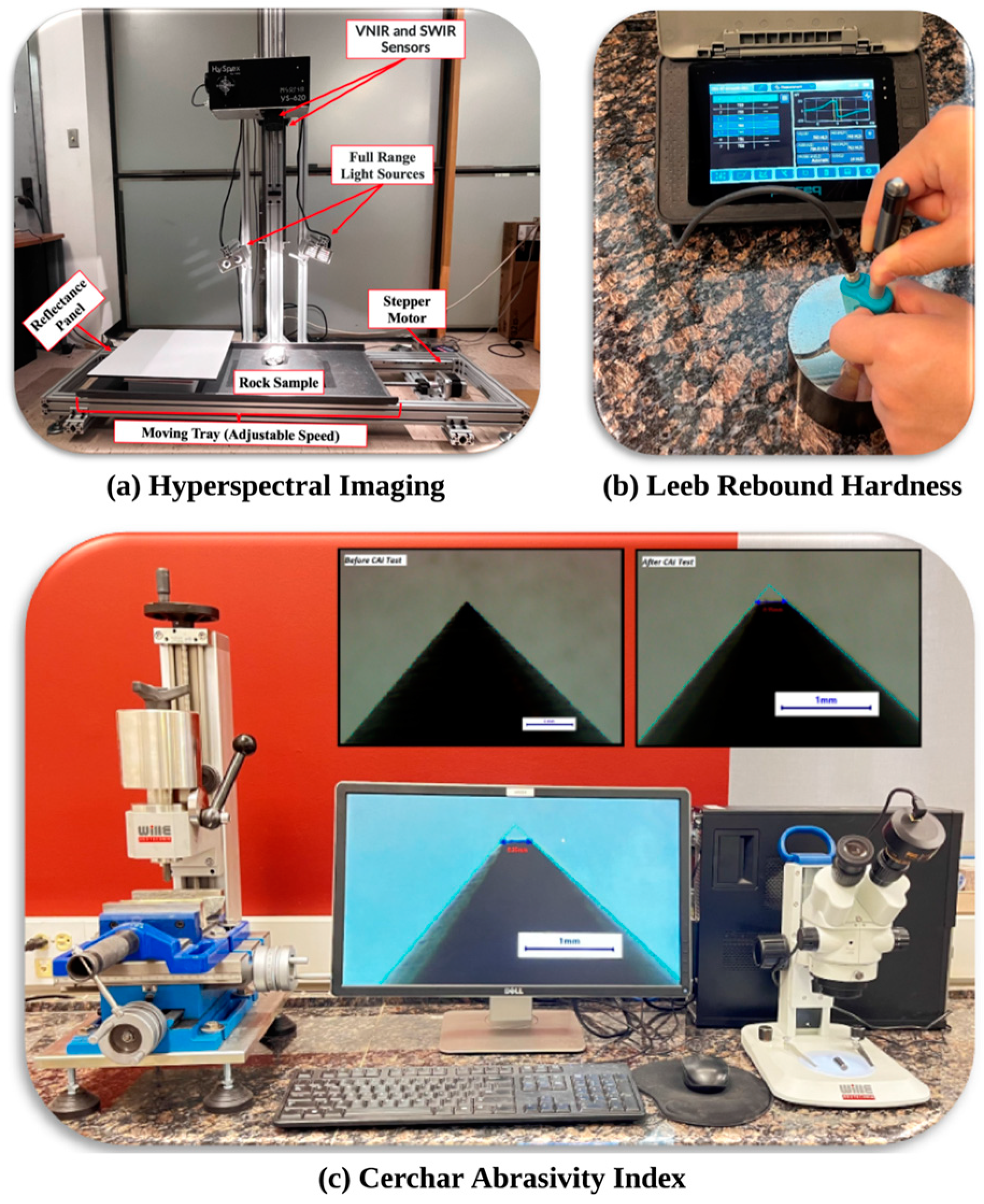Figure 3a details different parts of the designed hyperspectral imaging setup.

The differences in the rock types and mineralogical compositions of the collected rock samples could result in a wide range of albedo when scanning the sample in the lab. Three different diffuse reflectance panels with known spectral curves were used to ensure the proper scanning of the samples. The reference panels have 20, 50, and 90 percent nominal reflectance values. It also must be mentioned that the rock samples were scanned separately. The 20 percent diffuse reflectance panel was employed for darker samples, while the 90 percent was used for brighter samples.

In the second step, rock samples were subjected to the LRH test, a portable, fast, nondestructive dynamic impact-and-rebound test. LRH was originally developed to assess metallic materials’ hardness, and has recently been extensively applied to geoengineering projects [7,41,42,43,44,45,46]. The theoretical basis of the LRH test is based on the principle of energy consumption. In this test, the hardness value is reported as the ratio of the rebound velocity of a hard tungsten carbide spherical tip impact body to its impact velocity. While the impact velocity is always constant, the physicomechanical properties of the tested rock sample, such as surface elasticity and strength, act as a resistance factor and reduce the rebounding velocity [47].

LRH tests were conducted using an Equotip 550 Leeb D device (Proceq, Schwerzenbach, Switzerland) (Figure 3b) according to ASTM procedures and manufacturer testing guidelines [47,48]. For consistency, the term HLD will be used to report the hardness value measured by a D-type Leeb rebound device in this paper. An integrated approach based on the small sample theory and confidence interval was used to determine the representative mean HLD value for each sample [45]. Based on this approach, considering an error level and a specific confidence interval, one could find the minimum number of LRH measurements instead of performing a predefined number of measurements, resulting in the representative mean HLD value for each rock sample. Regarding calibration, it must be noted that the device was continually calibrated either after ten consecutive sample tests or at the beginning of the testing day.

CAI is one of the most used commonly abrasion tests for determining rock abrasivity and wear estimation on mechanical tools. As originally designed by the Center d’Etudes et Recherches des Charbonages (Cerchar) de France in the 1970s for coal mining applications, the test has gradually gained acceptance in other geoengineering fields, such as hard rock mining and tunneling [16,49,50]. The CAI test can be performed according to different standards, such as AFNOR. NF P 94-430-1 [51], ASTM D7625-10 [52], and ISRM [15]. Several modifications have been made to enhance the accuracy and practicality of the CAI test to date; among them, the original design developed by Cerchar Center and modified by West are the most widely used ones [16].

In this study, the CAI tests were performed using the West device employing pins of HRC 54 (Wille Geotehnik, Rosdorf, Germany) (Figure 3c). The device consists of a mechanical vice to firmly hold the specimen while a hardened steel stylus with a 90-degree cone tip interacts over the rock surface under a constant load of 70 N. Then, the rock sample moves under the stationary loaded stylus, ensuring a 10 mm scratch on the surface of the rock specimen. Testing was conducted on freshly broken rock surfaces resulting from the point load index test. However, CAI tests were conducted on saw-cut surfaces of rocks, which could not be broken using a point load device. A correction factor of 1.14 was used to account for the smooth surface produced by the saw cut, as recommended by ISRM [15]. The average of seven CAI tests was calculated for each specimen to measure the representative mean CAI value using the following equation:

$$\mathrm{CAI}=10\times {{\displaystyle \sum }}_{i=1}^7{d}_i$$

(1)

where $d_i$ is the average of measured wear on the stylus tip surface in two perpendicular profiles with an accuracy of 0.01 mm. A high-resolution calibrated camera mounted on a binocular microscope was used to measure the wear of the pins.

2.3. Data Preprocessing

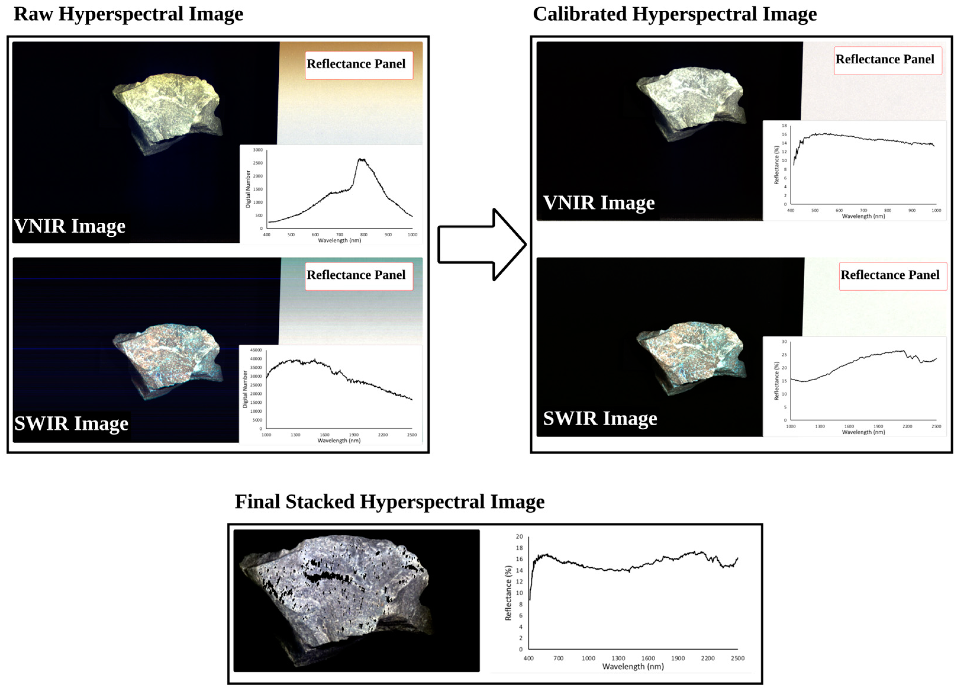
The preprocessing of raw data obtained from hyperspectral scanning involved four main steps. In the first step, the radiometric correction was applied to VNIR and SWIR scans, which included the reflectance calibration. It is important to note that the raw scan stores information about the amount of radiance reflected from the surface of the scanned rock sample. The reference panels considered material with known spectral curves and calibrated the reflectance values measured on the rock surface. The second step addressed the oversaturation problem, which occurs when the sensor cannot capture the amount of reflected energy in a single shot. There are two ways to deal with this problem. First, it can be prevented by adjusting the tray speed, reducing light intensity, and using an appropriate reflectance panel. However, in some cases, such as having bright minerals in very dark content, obtaining a high-quality scan of the darker part may lead to oversaturation in the brighter parts. Conversely, attempting to scan the brighter parts may result in noise scans of the darker portions. The second approach to dealing with oversaturation is to mask the oversaturated pixels and remove their values. During data collection, caution was taken to avoid oversaturation; however, oversaturation was inevitable in some of the samples for the sake of the spectral curve’s quality.

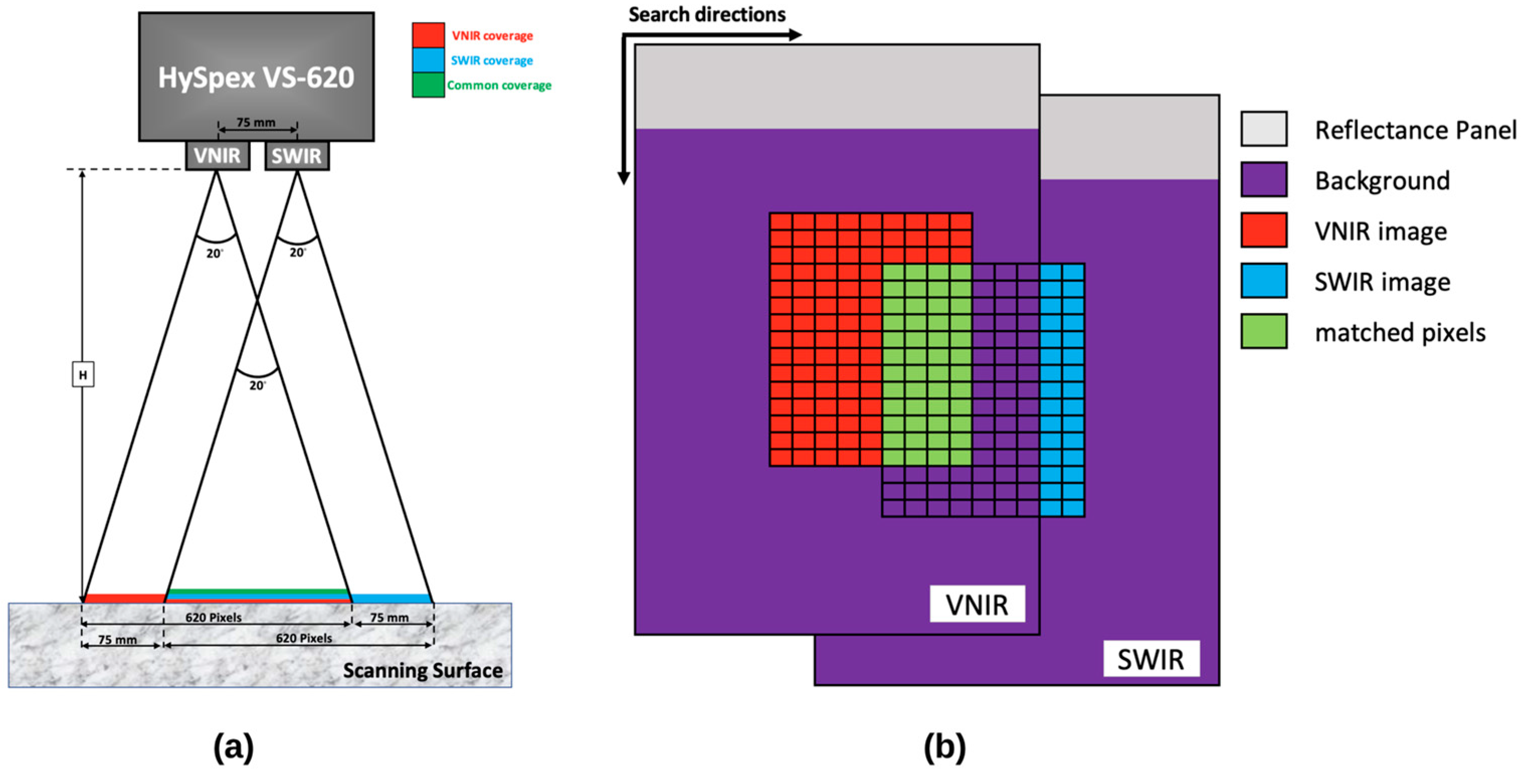
The third step was to stack the VNIR and SWIR scans. As was mentioned, the HySpex Mjolnir VS-620 can cover the full spectral range from 400 to 2500 nm using two hyperspectral sensors with different specifications. The VNIR sensor features a spectral resolution of 3 nm, covering the range from 400 to 1000 nm in 200 bands. In contrast, the SWIR sensor configures the range from 970 to 2500 nm in 300 bands, ensuring a spectral resolution of 5.1 nm. One way to address the difference in the obtained spectral resolutions is to resample at a desired spectral resolution when stacking images. On the other hand, while the spatial resolution of the VINR sensor is exactly double that of the SWIR one, these two sensors are not fully synchronized, resulting in the capturing of different lengths of images. This would result in having a few more lines in the VNIR image than in the SWIR image. Lastly, due to a baseline of 75 mm between the two sensors, their fields of view do not completely overlap, resulting in a common area smaller than the nominal coverage area for each sensor (Figure 4a). It must be noted that the common area’s size depends on the scanning distance (H). The shorter the scanning distance, the smaller the size of the common area.

These discrepancies prompted the need for the following preprocessing step, aimed at stacking these two hyperspectral images for further analysis. A Python algorithm was developed based on search theory and the maximum similarity between the two images to achieve this. Figure 4b demonstrates the concept behind the staking algorithm. As can be seen, the proposed algorithm tries to find the best match between two images by finding the maximum similarity between them. The algorithm was applied to all samples, resulting in a stacked image for each rock sample. It is worth noting that due to the overlapping of some part of the VNIR range with SWIR, the resulting stack image would contain 487 bands, slightly lower than 500 bands. The final preprocessing step focuses on cropping and removing background spectra to reduce the size of the stacked image. This is accomplished by limiting and cropping images to only the rock sample part. Figure 5 illustrates most of the preprocessing steps for one of the samples.

2.4. Train and Test Split

Data splitting is an essential step in developing machine learning (ML) models. It allows us to simulate the process of performance assessment by utilizing new data as we develop new models. To consider the testing dataset as unseen data, one simple requirement must be met: no information must leak into the development process from the testing dataset. Data leakage generally occurs during the data wrangling and exploratory data analysis (EDA) steps. For example, when the model is informed about the parameter range, data leakage occurs by knowing the information about the entire dataset. Therefore, it is obvious that the dataset must be split first to prevent any data leaks.

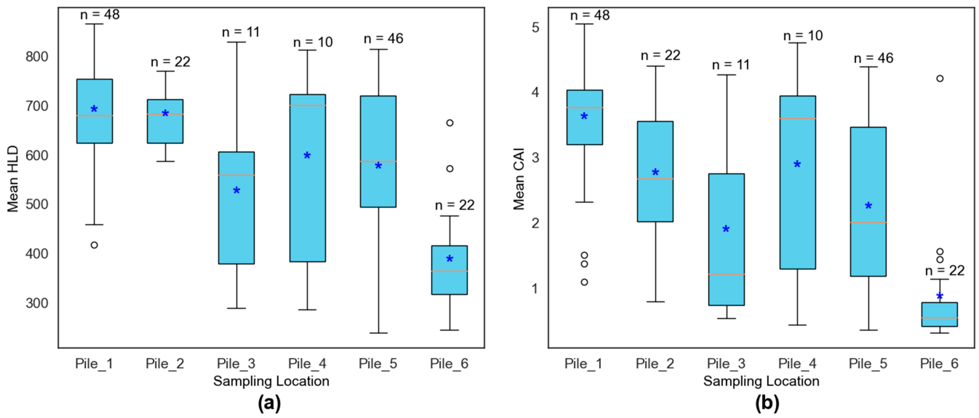
Datasets can be split in different ways depending on their characteristics. One of the most utilized approaches is the random split method, which is implemented to split the dataset by random shuffle. There could be two issues with using the random split. First, it is necessary to assess the split bias since 159 rock samples were collected at six different locations during the experimental stage. The random shuffle bias occurs when one data point is randomly selected as the training set, and its adjacent point is selected as the testing set, and this usually happens when data are geospatially correlated, such as core log data. It should be noted that the rock samples were randomly collected in different parts of blasted muck piles; therefore, it can be said that the collected samples are not geospatially related to each other.

Figure 6 shows the box plots of the mean HLD and CAI values of rock samples from each sampling location. In Figure 6, blue asterisks represent the mean value of the sampling location. In addition, the number of samples taken from each location is also shown above each box plot. Variation within the collected samples at each location can be seen for both mean HLD and CAI, indicating no geospatial correlation. Otherwise, each sampling location should have tighter box plots with lower variation.

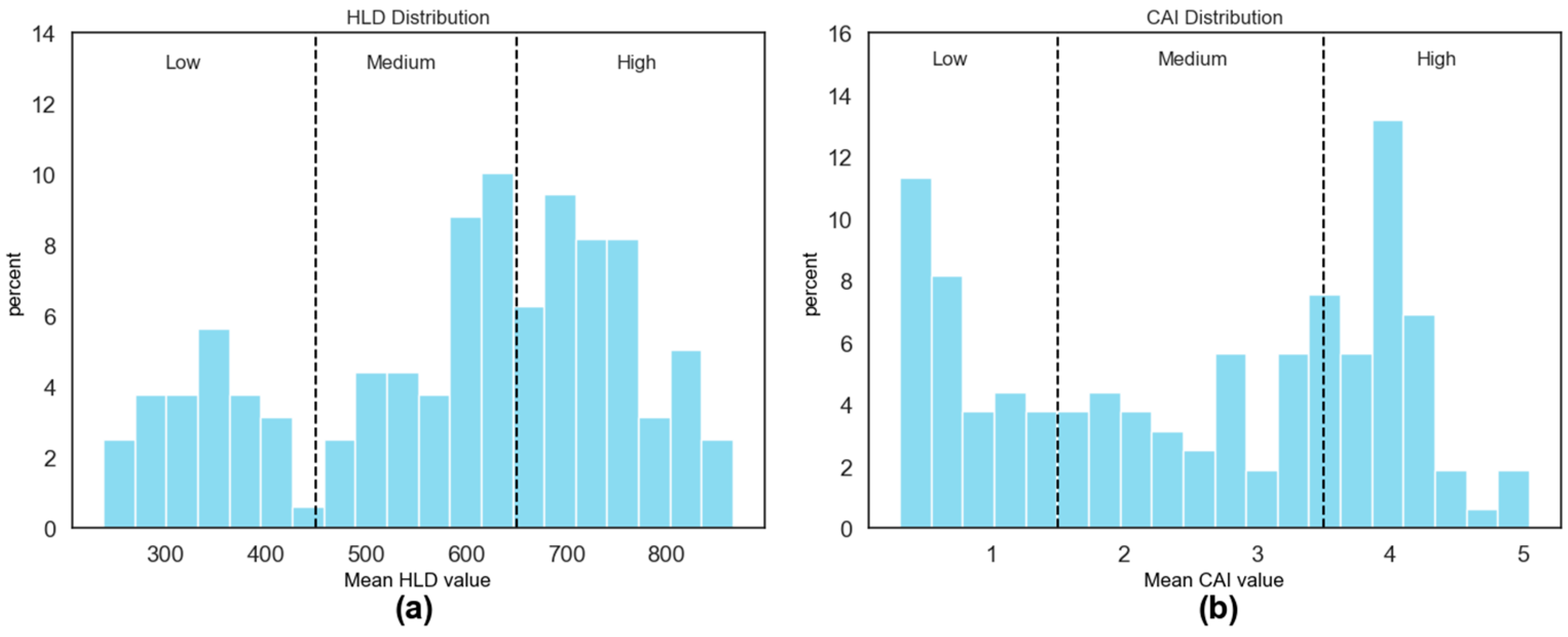
Secondly, imbalanced data may occur, which refers to the situation in which the data are not evenly distributed across the entire range of the target parameter. In this case, most data would be found in a certain range, while the remaining parts would have less data. Data imbalances can negatively affect the performance of predictive models since, typically, the more data that are introduced to a model, the better it performs. Therefore, if there is insufficient data for a specific range of the target parameter, the model cannot perform perfectly for that range. Various techniques can be used to address this issue, such as obtaining more data, which can be time-consuming and expensive. This study uses class weighting methods to ensure there is a similar ratio between the different classes in the training and testing dataset. 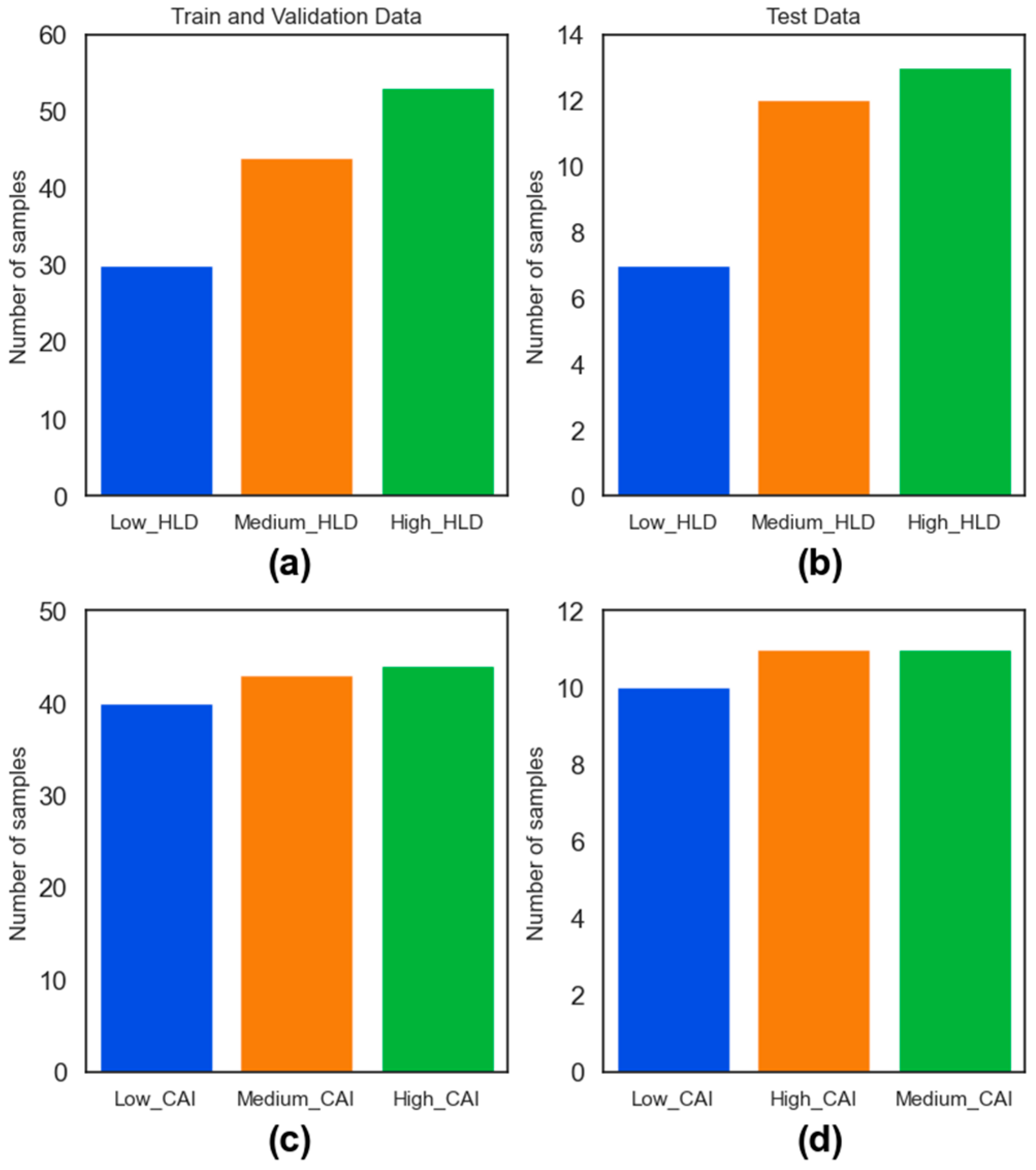As shown in Figure 7, two auxiliary thresholds are applied for both mean HLD and CAI values, dividing the distributions into three groups (low, medium, and high). For the HLD distribution, 450 and 650 are considered thresholds, and 1.5 and 3.5 are considered thresholds for the CAI distribution. It should be noted that these classes will only be used during the train and test split. As can be seen in Figure 8, the results of the random split addressing class imbalance for both HLD and CAI values are presented. In this study, 80 percent of the collected rock samples (127 rock samples) were considered for the training, and the remaining 20 percent (32 rock samples) were used only for performance assessment as unseen data.

2.5. Feature Extraction and Exploratory Data Analysis

One of the greatest challenges in developing predictive models using hyperspectral data is dealing with their high dimensionality. For instance, in this research, the final scan of each rock sample contains around 50,000 pixels with 487 channels each. Generally, developing machine learning or deep learning models using raw hyperspectral data requires more than thousands of records, which are impossible to collect in the field of geoengineering.

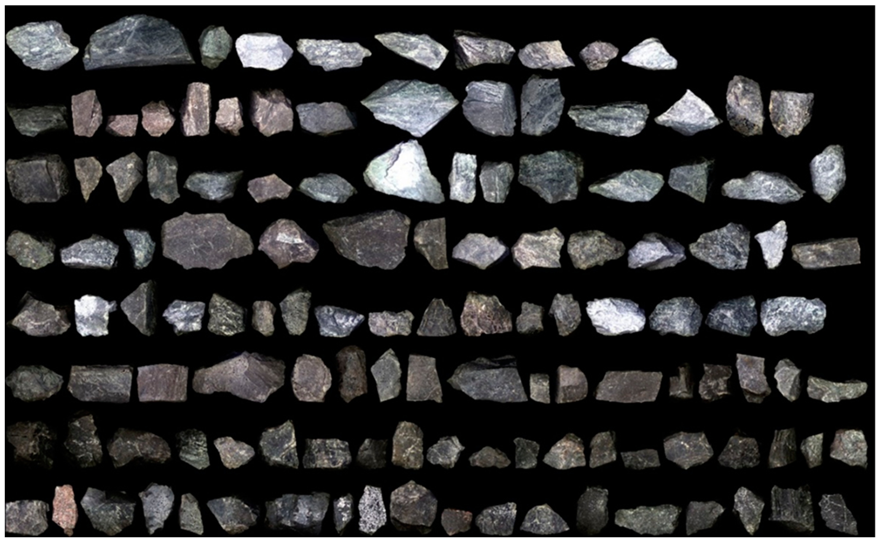
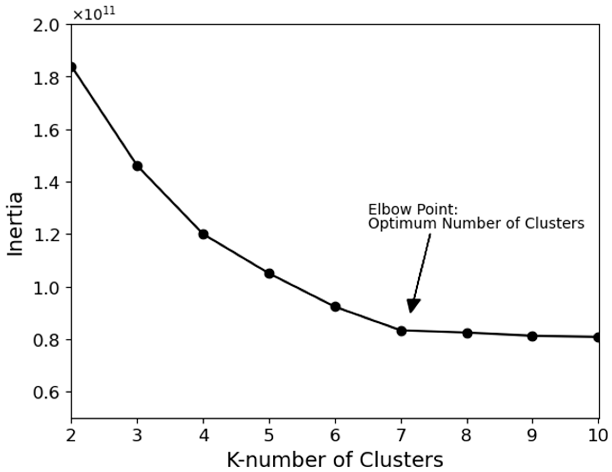
This study uses a feature extraction approach based on K-means clustering and the band ratio concept to extract the most important features. This section details the proposed feature extraction approach. The first step was to mosaic all stacked images of the training dataset. Figure 9 demonstrates the true RGB of the mosaic image used for the feature extraction purpose. Afterward, a K-means clustering was applied to this image to obtain the dominant spectral curves. The elbow method was employed to determine the optimum number of clusters. Hence, several K-means analyses with different numbers of clusters ranging from 2 to 10 were performed. 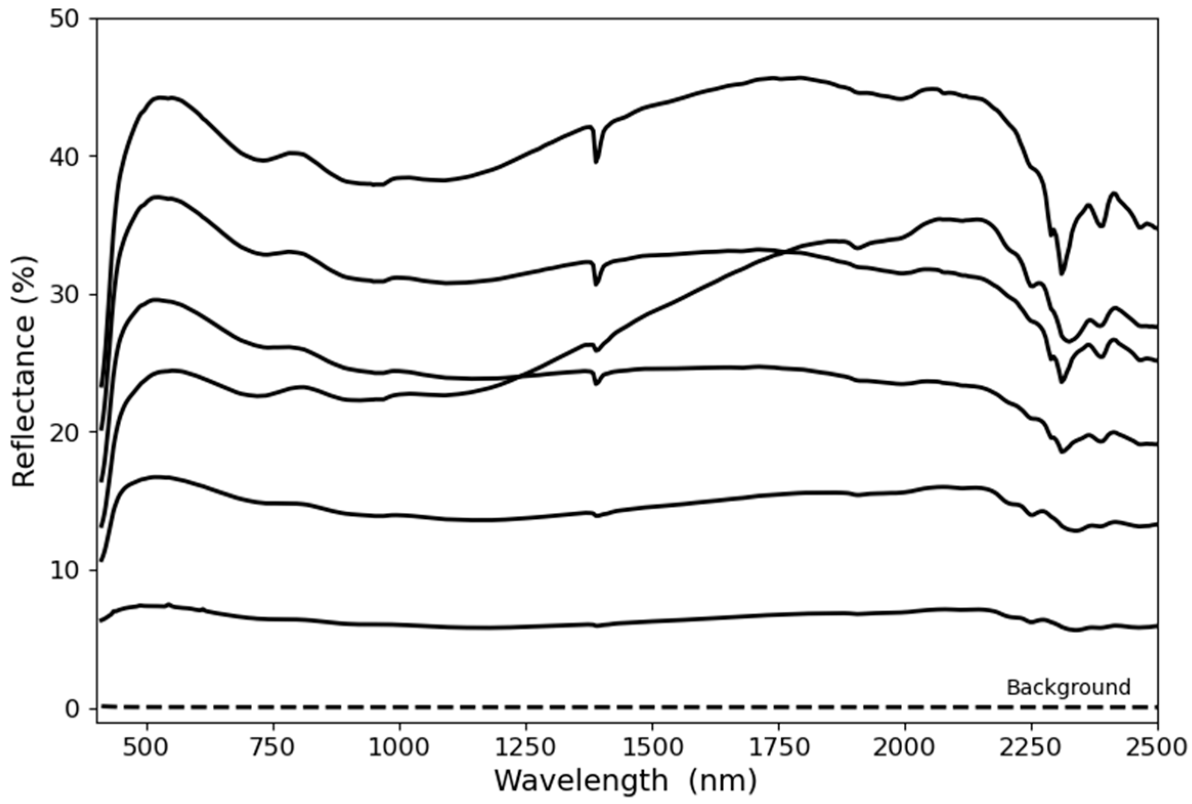As shown in Figure 10, a K-mean clustering with 7 clusters is the optimum way to obtain the dominant spectral curves. The mean spectral curves resulting from the K-means clustering with 7 clusters are shown in Figure 11. It should be noted that one of the spectral curves belongs to the image background and was excluded.

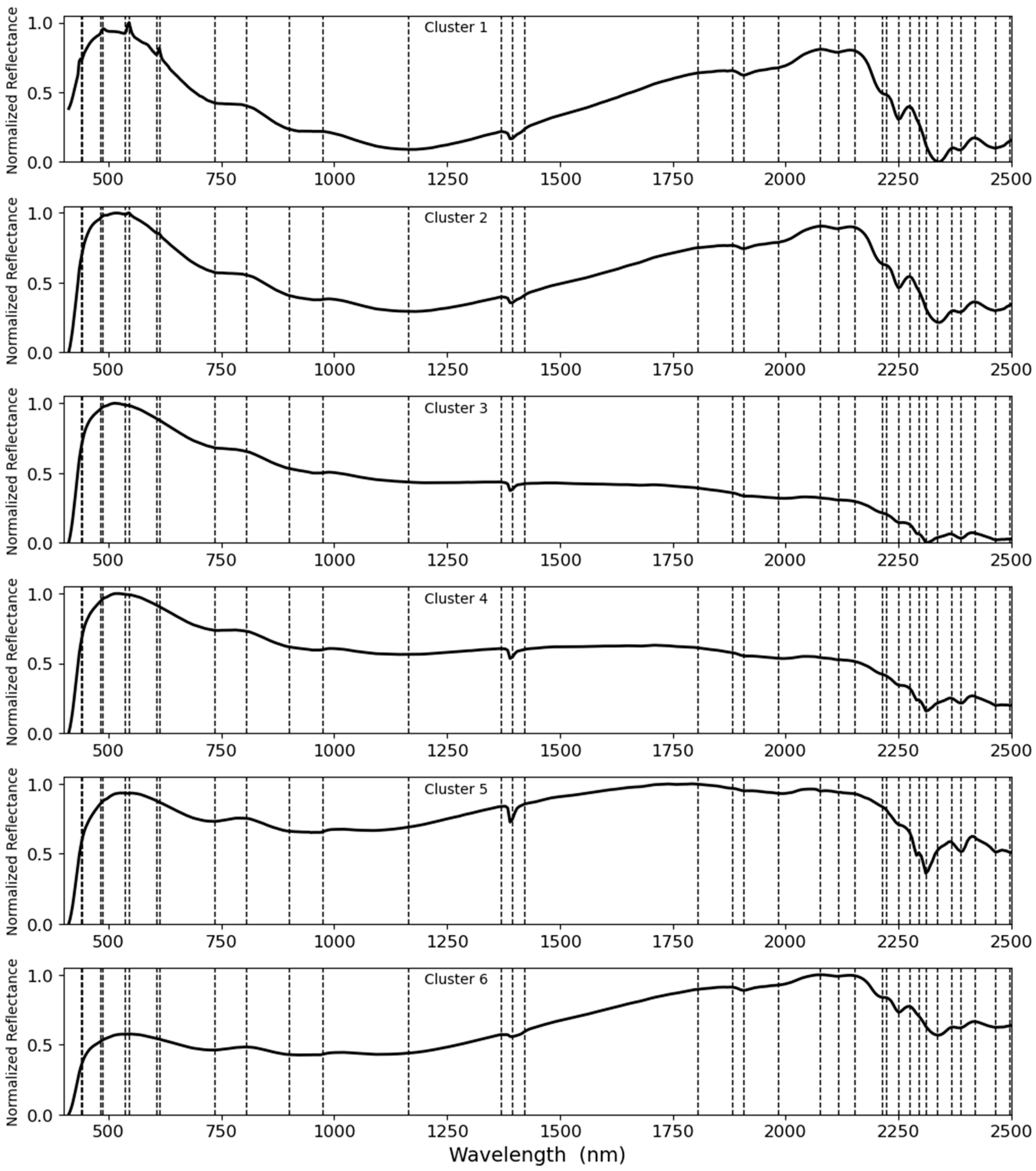
After retrieving the dominant spectral curves resulting from the K-means analysis, all six spectral curves were normalized and carefully studied for absorption peaks, reflectance peaks, and changes in slope. A feature was defined as a band ratio whenever a change was observed in the curves. Figure 12 shows the process of feature extraction.

Table 2. The obtained band ratios from the feature extraction approach.

Features	Band1	Band2	Source	Features	Band1	Band2	Source
F_1	437	440	VNIR	F_15	1420	1804	SWIR
F_2	481	487	VNIR	F_16	1880	1906	SWIR
F_3	440	487	VNIR	F_17	1983	2075	SWIR
F_4	536	545	VNIR	F_18	2075	2116	SWIR
F_5	606	612	VNIR	F_19	2116	2152	SWIR
F_6	551	603	VNIR	F_20	2152	2213	SWIR
F_7	621	734	VNIR	F_21	2213	2223	SWIR
F_8	734	804	VNIR	F_22	2223	2249	SWIR
F_9	804	900	VNIR	F_23	2249	2274	SWIR
F_10	900	975	VNIR	F_24	2295	2310	SWIR
F_11	975	1164	SWIR	F_25	2310	2336	SWIR
F_12	1164	1369	SWIR	F_26	2336	2366	SWIR
F_13	1369	1394	SWIR	F_27	2387	2418	SWIR
F_14	1394	1420	SWIR	F_28	2464	2494	SWIR

provides information regarding the obtained band ratios for further analysis. In the next step, the approach was applied to all samples, reducing the dimensionality from an order of 487 to 28. For each sample, the main representative feature values were considered as the mean of the features over all pixels, and the resultant dataset was used for developing the predictive models.

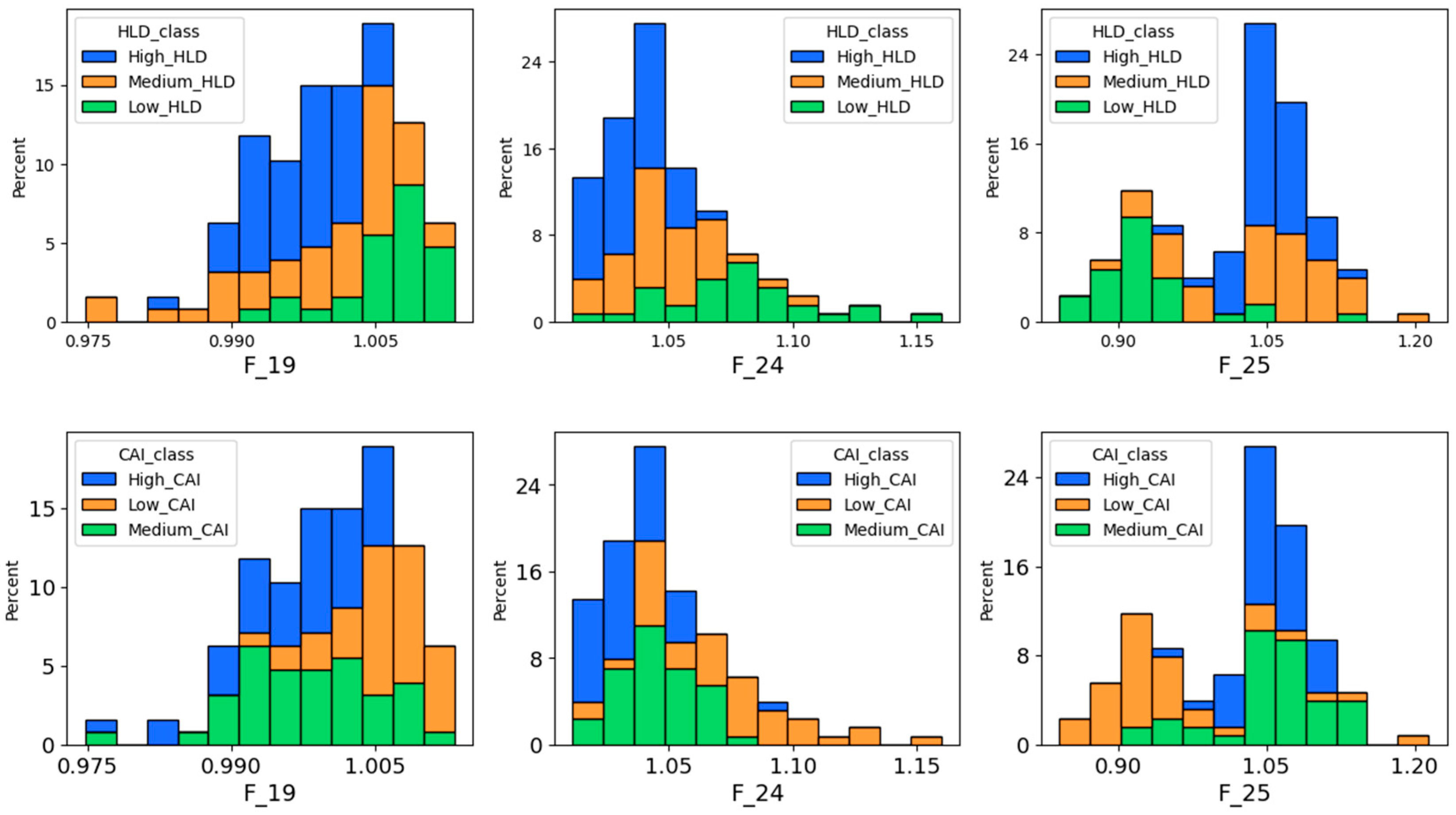
To explore and understand the relationship between the selected band ratios, as the input features, and HLD and CAI values, as the target parameters, the correlation between them was explored. Figure 13 illustrates the pairwise correlation matrix of the selected band ratios and HLD and CAI values. The absolute correlation between each feature was considered to make the interpretation easier. In this case, while 0, represented by blue, indicates no linear relationship, 1, represented by green, indicates a perfect linear relationship. Although there could be strong correlations between some of the band ratios, the pairwise matrix reveals moderate correlations between some of the band ratios with the target parameters, i.e., HLD and CAI. To better understand these relations, the distribution of each feature concerning HLD and CAI classes was studied (Figure 14). It must be noted that the HLD and CAI classes were defined based on the auxiliary thresholds established in the previous section. As can be seen, certain selected features, such as feature 25 (F_25), exhibit a trend towards HLD and CAI classes. However, a meaningful relationship could not be observed for most of the selected features. It is worth noting that these distribution graphs were developed using the training dataset, and the testing dataset is yet to be revealed.

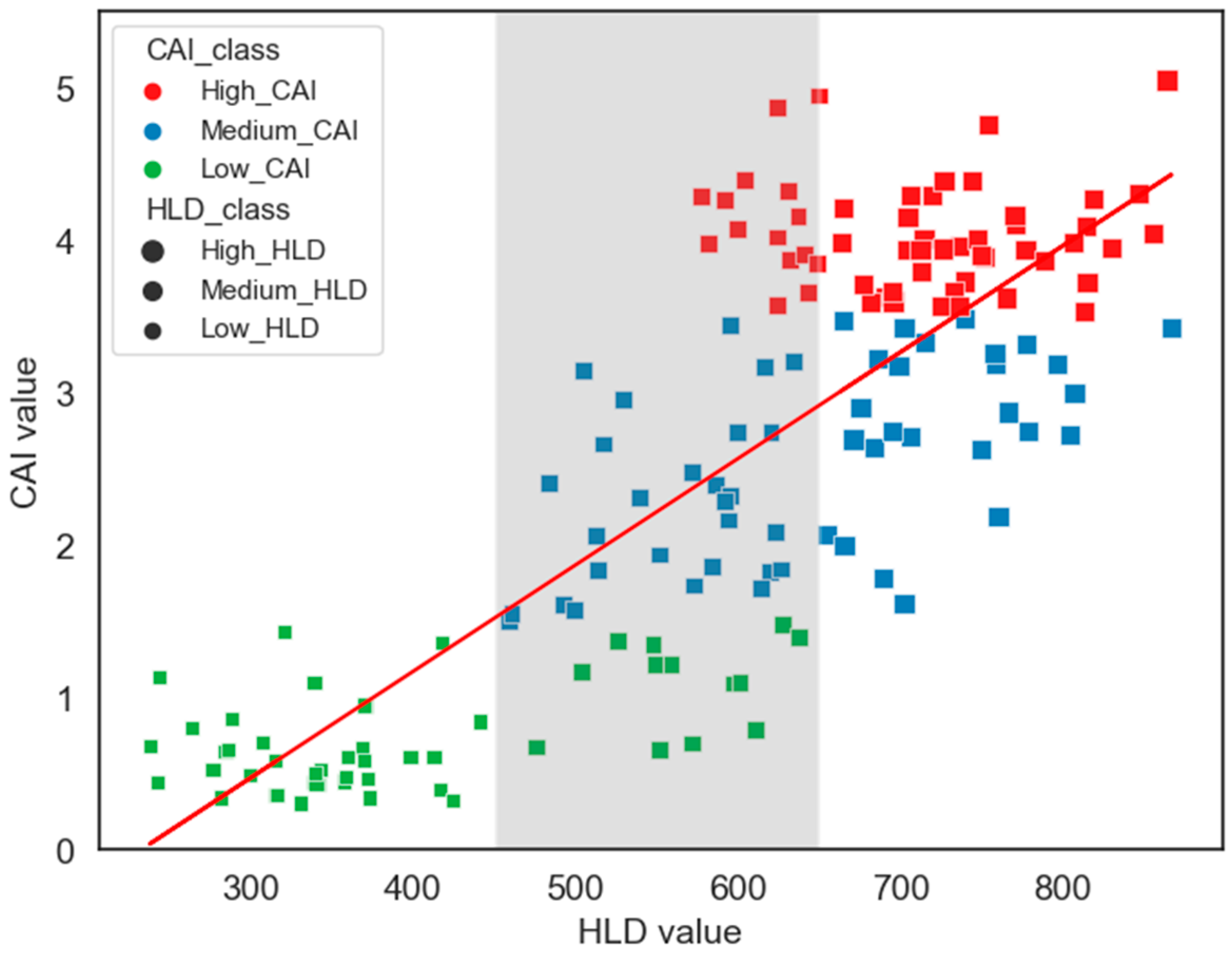
In Figure 13, a good correlation between HLD and CAI values can also be observed, which has a great deal of significance. Figure 15 provides a scatter plot of HLD and CAI values to better analyze this correlation. As can be seen, there is a noticeable linear relationship between HLD and CAI values. This aspect bears significance as establishing dependence between HLD and CAI could facilitate the development of a unified predictive model capable of simultaneously estimating both HLD and CAI values. To better understand their relationship, HLD and CAI values were categorized into three distinct groups using a similar approach used in the train and test split stage. A three-color system was used to distinguish between different classes of CAIs. In contrast, HLD classes were identified by varying marker sizes: the bigger the marker, the higher the HLD value. Despite the notable correlation, the relationship between HLD and CAI values is not quite clear. For instance, in the range 450 to 650 of HLD value, associated with medium hardness, CAI values range from 0.5 to 5, comprising all CAI classes. Therefore, separate predictive models were developed for each hardness variable instead of developing a unified predictive model capable of estimating both HLD and CAI values simultaneously.

2.6. Developing Predictive Models

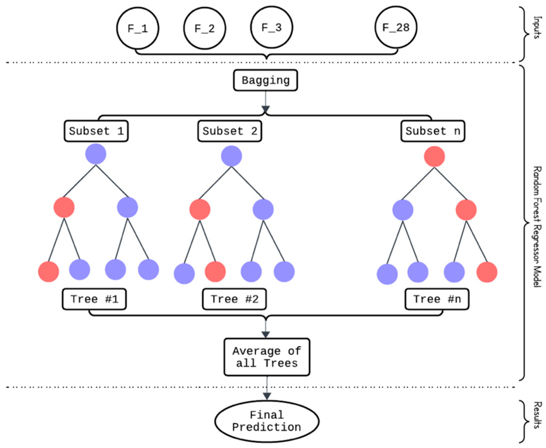
The random forest regressor (RFR) algorithm was employed to develop predictive models for HLD and CAI values based on hyperspectral data. This section explains the theoretical concept behind the RFR algorithm and the steps taken to tune it.

A random forest (RF) algorithm is an ensemble learning algorithm that can handle both classification and regression tasks [54]. The term ensemble learning refers to a method for combining predictions from multiple machine learning algorithms, called base learners. In the case of the RF algorithm, numerous decision trees are applied to different subsets of a dataset, leading to higher precision estimations. Using multiple trees overcomes the instability and substantial variability that can arise when using individual decision tree models. This leads to inconsistent generalization behavior even with insignificant changes in the dataset [55]. In fact, by forming an ensemble model from independent individual trees, one could expect more robust predictions.

For each decision tree within the RF algorithm, the data are recursively divided into more homogeneous groups, called nodes, aiming to enhance the predictability of the response variable [56]. A split is determined by the values of predictor variables with significant explanatory factors. Then, an RF model is constructed by training multiple decision trees on different bootstrapped subsets of the data. In the case of the regression analysis, the final predicted value is the mean of the fitted responses from all the individual decision trees generated by each bootstrapped sample. The foundational principles and formulations underlying the RFR are elaborated upon by [54]. Figure 16 schematically demonstrates the structure of the RF regressor algorithm.

The performance of machine learning algorithms is directly controlled by the hyperparameters, and one must first find the optimal hyperparameter values to obtain the best performance on a given dataset. This process is called hyperparameter tuning and can be categorized into uninformed and informed methods [57]. Uninformed hyperparameter tuning involves systematically exploring a predefined set of hyperparameter values without leveraging any information about the model’s performance. There are different uniformed hyperparameter tuning methods, such as grid search or random search. In grid search, the hyperparameter space is discretized into a grid, and the model is trained and evaluated for each combination of hyperparameters. While grid search is exhaustive, it can be computationally expensive and may not be efficient when dealing with high-dimensional hyperparameter spaces. To address this problem, a random search approach was proposed, which found that for most datasets, only a few hyperparameters matter. However, Bergstra and Bengio [58] showed that random search becomes unreliable as the complexity of the model increases.

Informed hyperparameter tuning, on the other hand, utilizes information gained during the tuning process to guide the search more efficiently. Bayesian optimization (BO) is a popular method in this category. In this situation, the tuning process could be considered as an optimization problem, and since the objective function is unknown, traditional techniques, such as gradient descent, cannot be applied. BO is a highly effective technique for solving optimization problems that do not have a closed-form objective function [59,60]. Optimization involves using prior information about the unknown objective function and sample information to determine the posterior distribution of the function. The objective function can eventually be optimized based on this posterior information [61]. This study uses BO based on the Gaussian process to tune hyperparameters of the RFR algorithm. A complete guide on how BO has been used in this study for hyperparameter tuning can be found in [57]. The following section explores the results of the predictive models and assesses their performance

3. Results and Discussion

In this study, the RFR algorithm was used to develop models for predicting HLD and CAI values using VNIR and SWIR data. This section presents the obtained results for each model and then provides a comprehensive performance assessment of the models. To achieve this, several statistical evaluation indices, including coefficient of determination (R²), root mean square error (RMSE), and variance account for (VAF) between the measured and predicted values, are employed for evaluating the accuracy of the predictive models. A model is considered ideal when R² is 1, RMSE is 0, and VAF is 100%. The following formulas for calculating the mentioned indices are presented in Equations (2)–(4).

$$R^2=1-{\displaystyle \frac{SSR}{SST}}$$

(2)

$$RMSE=\sqrt{\left({\displaystyle \frac{1}{N}}\right){\displaystyle \sum }_{i=1}^N{\left(A_i-P_i\right)}^2}$$

(3)

$$VAF=\left[1-{\displaystyle \frac{var\left(A_i-P_i\right)}{var\left(A_i\right)}}\right]\times 100$$

(4)

where SSR, SST, $A_i$, $P_i$, and N are sum squared regression, the sum of squares total, the actual value of ith sample, the predicted value of ith sample, and the number of samples used for testing models, respectively.

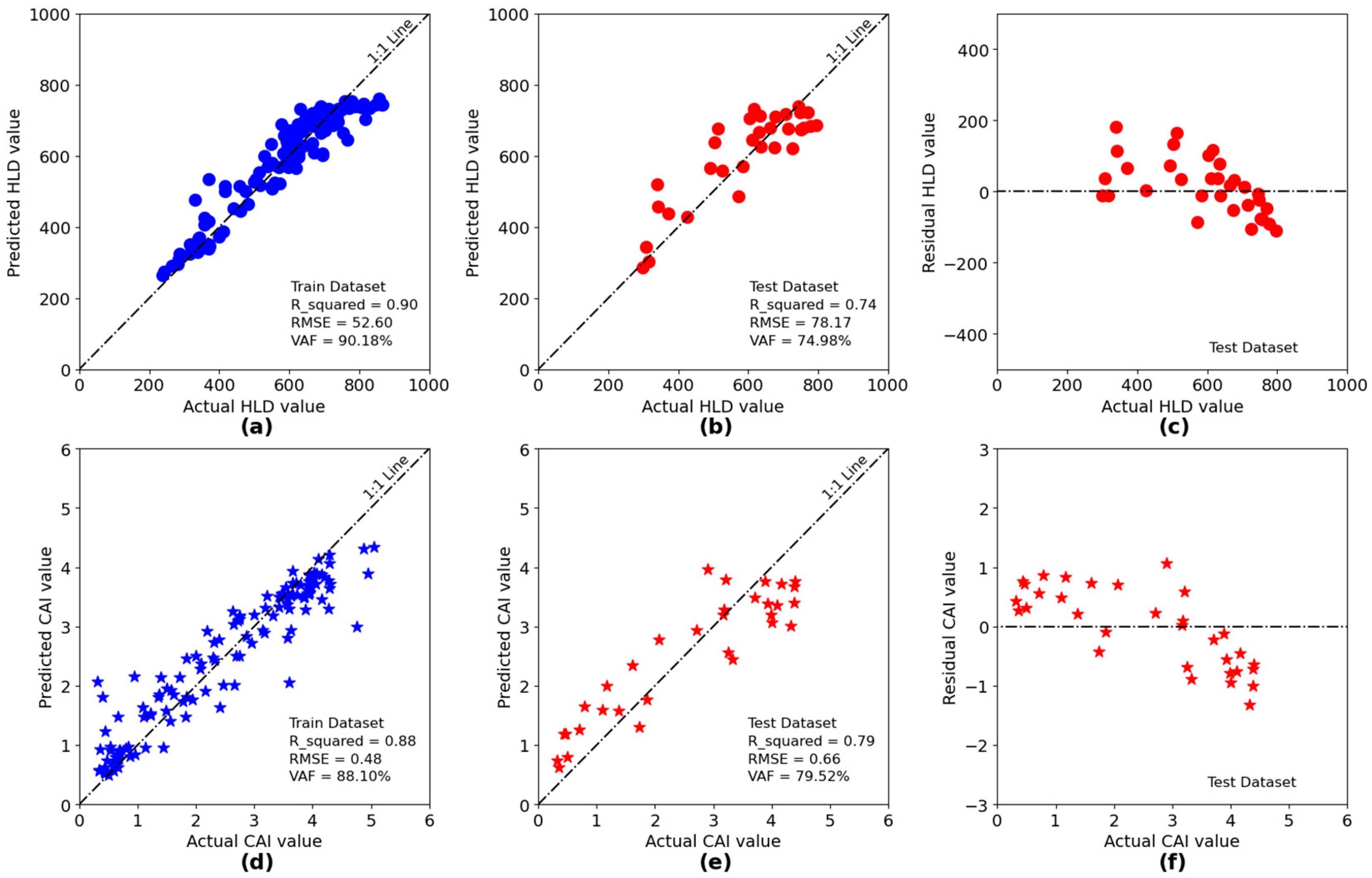
As mentioned before, 32 records representing 20 percent of datasets, which were not incorporated in the development/training of the predictive models, were considered for testing the developed models. Figure 17 illustrates the performance evaluation for the developed models. A 1:1 plot between the actual and predicted values provides a concise and straightforward way to evaluate the performance of predictive models. The closer the data to the 1:1 line, the better the performance of the model. In addition, in the case of projecting actual and predicted values on horizontal and vertical axes, respectively, data points located under and above the 1:1 line represent under- and overestimation, respectively. As can be seen on the testing dataset, Figure 17b,e, the data are well scattered around the 1:1 line.

Regarding the performance comparison, the developed model of CAI with an R² of 0.79 performs slightly better than the developed model for HLD with an R² of 0.74. Considering the hyperspectral data as nondestructive remotely sensed data, the obtained results are promising. In addition, Figure 17c,f show the residual plot between actual and predicted values for HLD and CAI models as a graphical means for analyzing the pattern of differences between actual and predicted values. In the ideal case, the residual plot should be randomly distributed around the $residual value=0,$ and no clear pattern should be observed. Evidently, no pattern can be observed in both cases, confirming that the predictive model is performing well, and the residuals are randomly distributed around zero.

The impact of input features on the performance of the developed models for predicting HLD and CAI values was studied using the concentration approach by SHAP analysis, which is a method that explains the output of machine learning models by attributing the contribution of each feature to the final prediction. It uses game theory to fairly distribute the “credit” of the prediction among the input features, making it easier to understand which features are most influential [62]. The obtained results could be used as the predictive power indicator of input features. With this, we can gain more insight into the problem and select features when there are too many variables for further studies. 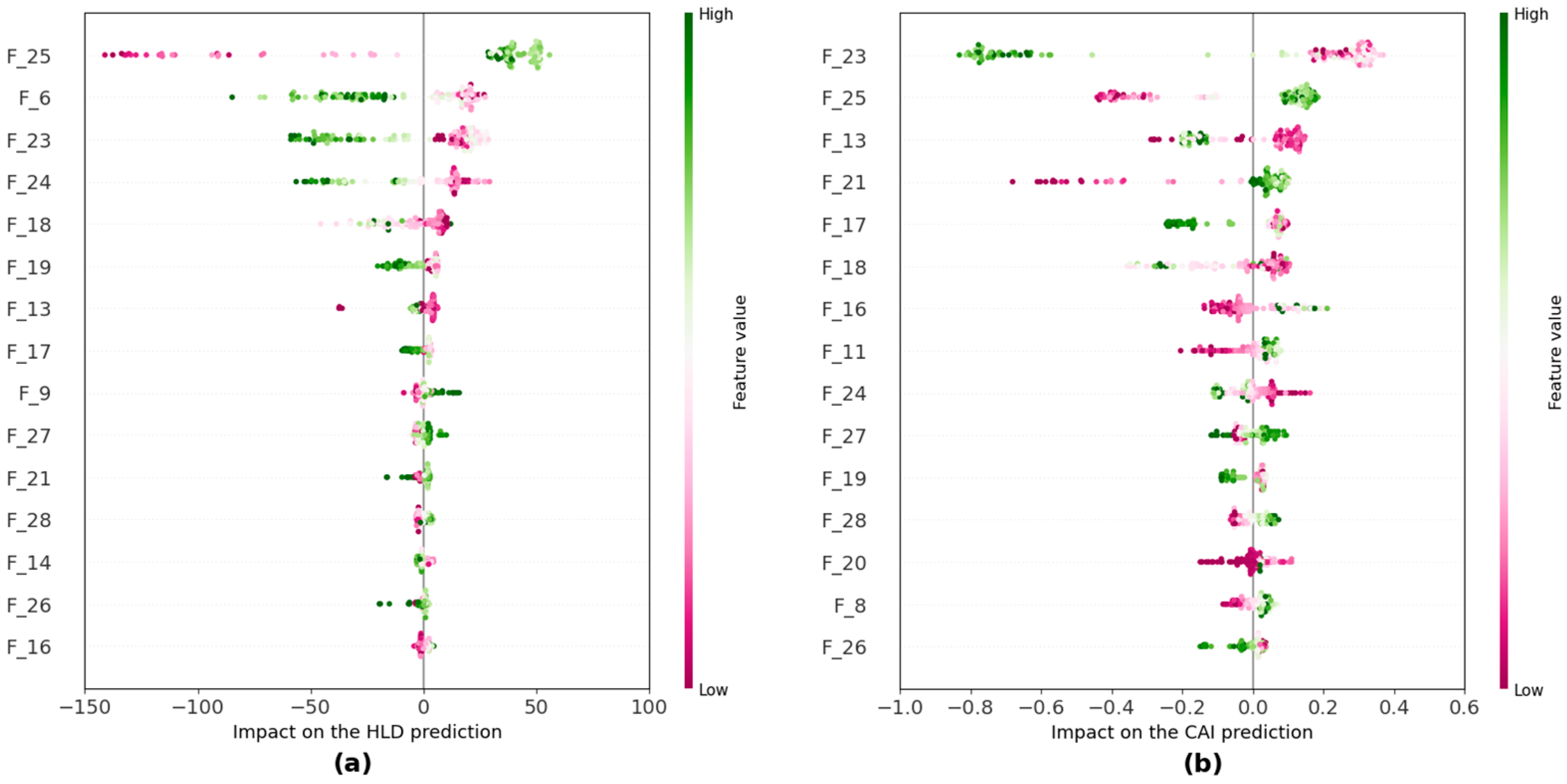Figure 18 shows the results of SHAP analysis on the predictive models for the top 15 features in each case. Red represents the lower value, and light green represents the higher value of each input feature. Regarding the degree of importance, the wider the distribution of the input feature, the greater the impact on the prediction. It should also be noted that the top 15 features are sorted from most to least predictive on the vertical axis, from top to bottom. Based on Figure 18, “F_25”, “F_6”, “F_23”, and “F_13” are among the most influential input features for both HLD and CAI. As can be seen, the higher the “F_25”, the higher both the predicted HLD and CAI values.

In addition, when referring to Table 2, the obtained band ratios from the feature extraction approach, one can easily see that the most important features are located within the SWIR region in both HLD and CAI cases. This aspect bears significance, as establishing accurate predictive models solely based on either VNIR or SWIR data could significantly enhance the practicality of the proposed method by reducing the dimensionality of the scanning data and speeding up the data processing. Therefore, an attempt was made to develop separate predictive models based solely on VNIR or SWIR and compare their performance with the initial case, i.e., predictive models based on VNIR and SWIR data. 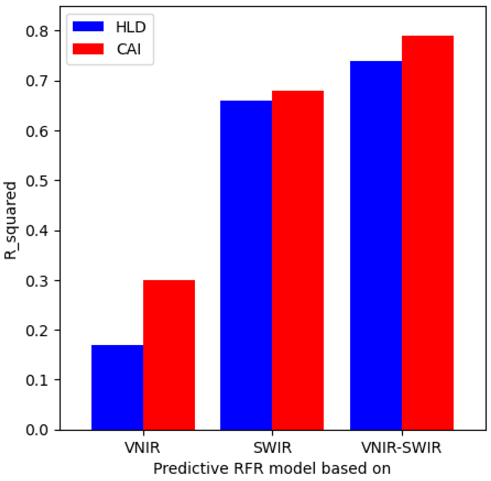Figure 19 illustrates the R² of different models on the testing dataset. Although the performance of the SWIR-based models is slightly lower than the initial case, the results of VNIR-based models are not within the acceptable range. In addition, for all three different situations, it was observed that the predictive models perform slightly better for CAI compared to HLD values, also highlighted in

Table 3. The performance assessment of HLD and CAI predictive models developed based on VNIR, SWIR, and VNIR-SWIR.

Model Developed Based on	R2		RMSE		VAF (%)
	HLD	CAI	HLD	CAI	HLD	CAI
VNIR	0.17	0.30	139.8	1.21	17	31
SWIR	0.66	0.68	88.4	0.81	67	68
VNIR-SWIR	0.74	0.79	78.2	0.66	75	80

.

The hyperspectral data used in this study for developing predictive models were acquired in a controlled laboratory environment, with ideal illumination, no moisture content, no atmospheric effects, and constant scanning distance, which could differ from the field conditions. Because such parameters could significantly affect the quality of hyperspectral data [63], investigating their effects on the performance of the developed models is of vital importance for developing more robust predictive models based on field conditions. It is recognized that the conditions mentioned above might affect the results of the developed predictive models based on field data.

Illumination generally affects the spectral intensity and does not significantly alter the spectral shape. Odermatt and Gege [64] investigated the effects of sun angle on the spectral curve and showed that a change in sun angle could only result in a change in spectral intensity. Similar results also can be observed in [65]. On the other hand, Philpot and Tian [66] studied the effects of soil water content on the spectral reflectance curves and explained that while the higher water content results in a lower intensity of the spectral curve, the shape of the spectral curve is almost the same.

The other factor affecting the quality of the hyperspectral images is the scanning distance (H), the distance between the sensors and the scanning surface, as shown in Figure 4a. This distance is longer in the field and can affect the spatial resolution of the scanned data. This factor could affect the hyperspectral images in two ways. First, the longer the scanning distance, the bigger the pixel size, which means more mixing of the spectral curves. Secondly, in field practices, increasing H would increase the potential for greater atmospheric effects. It must be noted that this study does not address the uncertainties associated with the atmospheric condition and only focuses on the effects of spatial resolution on the proposed approach. Regarding the effects of different pixel sizes, i.e., different scanning distances, a resampling approach was used to simulate the situation of scanning the collected rock samples from different H. The main reason for following such an approach is that it was not possible to increase the actual distance between VS620 and rock samples in the lab due to the lab rack’s limitations.

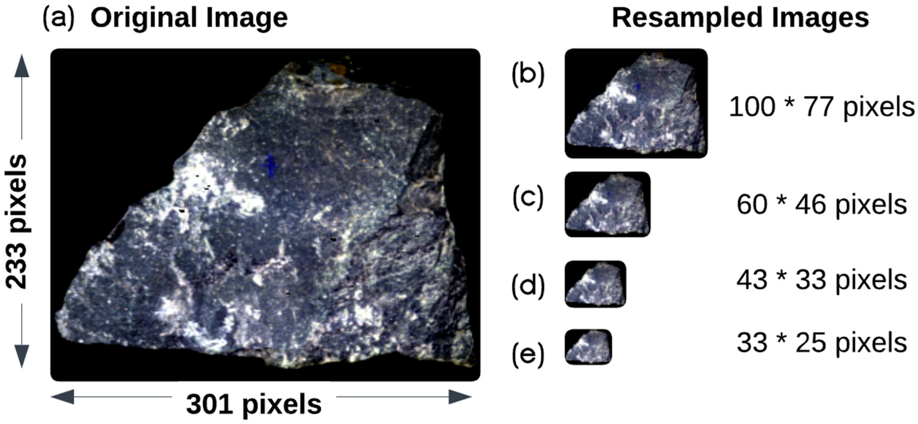
The utilized resampling approach consists of three steps: (1) considering a specific window size, (2) averaging the spectral curves within the window size, and then (3) assigning the average spectral curve to the new pixel. Four different window sizes, ranging from 1 to 4, were considered for the resampling purposes, representing a scanning distance ranging from 3 m to 9 m. A window size of 1 means considering a tile of 3-by-3 pixels of the original image and assigning the mean spectral value of that tile to a pixel in the new image. In this case, the pixel size will increase from 0.57 mm by 0.57 mm in the original image to 1.71 mm by 1.71 mm in the resampled image. It must be noted that the window size of 1 simulates the hyperspectral scanning from a scanning distance of 3 m. More detailed information regarding the considered window sizes is mentioned in

Table 4. The parameters considered in the employed resampling approach.

Reshaped Image	Pixels within the Window	Equivalent H (m)	New Pixel Size (mm2)
Window size of 1	3 × 3	3	1.71 × 1.71
Window size of 2	5 × 5	5	2.84 × 2.84
Window size of 3	7 × 7	7	3.98 × 3.98
Window size of 4	9 × 9	9	5.11 × 5.11

.

The resampling approach was only applied to the testing dataset, and the main reason for doing so was to see whether the lab-based predictive models could be applied in the field conditions or not. In fact, the scanning distance was tried to see how it could impact the proposed feature extraction approach and the performance of predictive models. Figure 20 shows the results of the resampling approach on sample GS1-17. 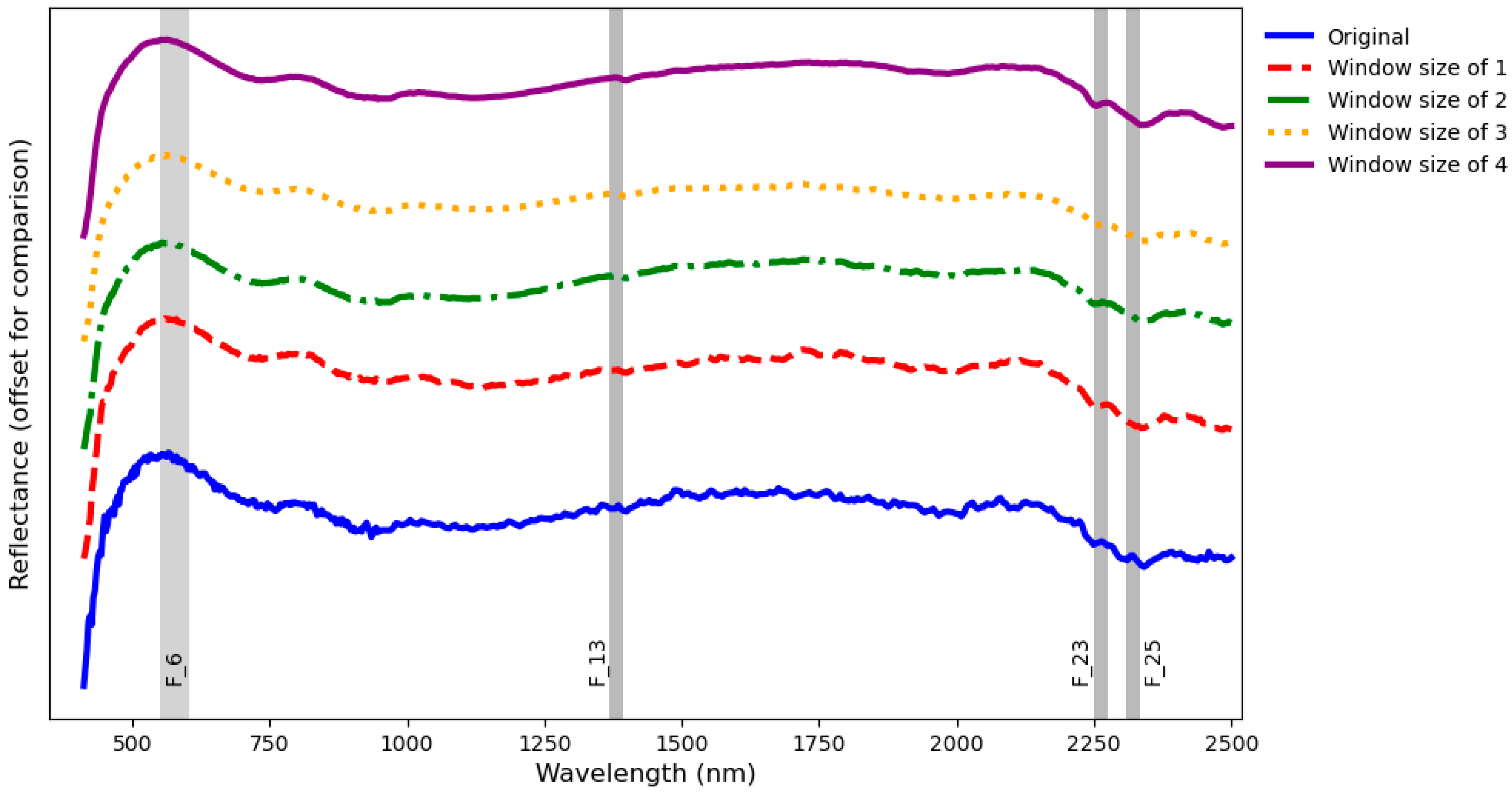To better illustrate the effects of the resampling approach on the spectral curve, Figure 21 compares the spectral curves of the specified spot in Figure 20 for the original and different resampled images. It is worth noting that spectral curves are shifted upward for better comparison only. As can be easily seen, the general trends of all spectral curves are the same, and the only obvious difference is that as the order of window size increases, the obtained spectral curves tend to be smoother. In addition, Figure 21 shows the four most influential extracted features of the proposed models (F_25, F_23, F_13, and F_6).

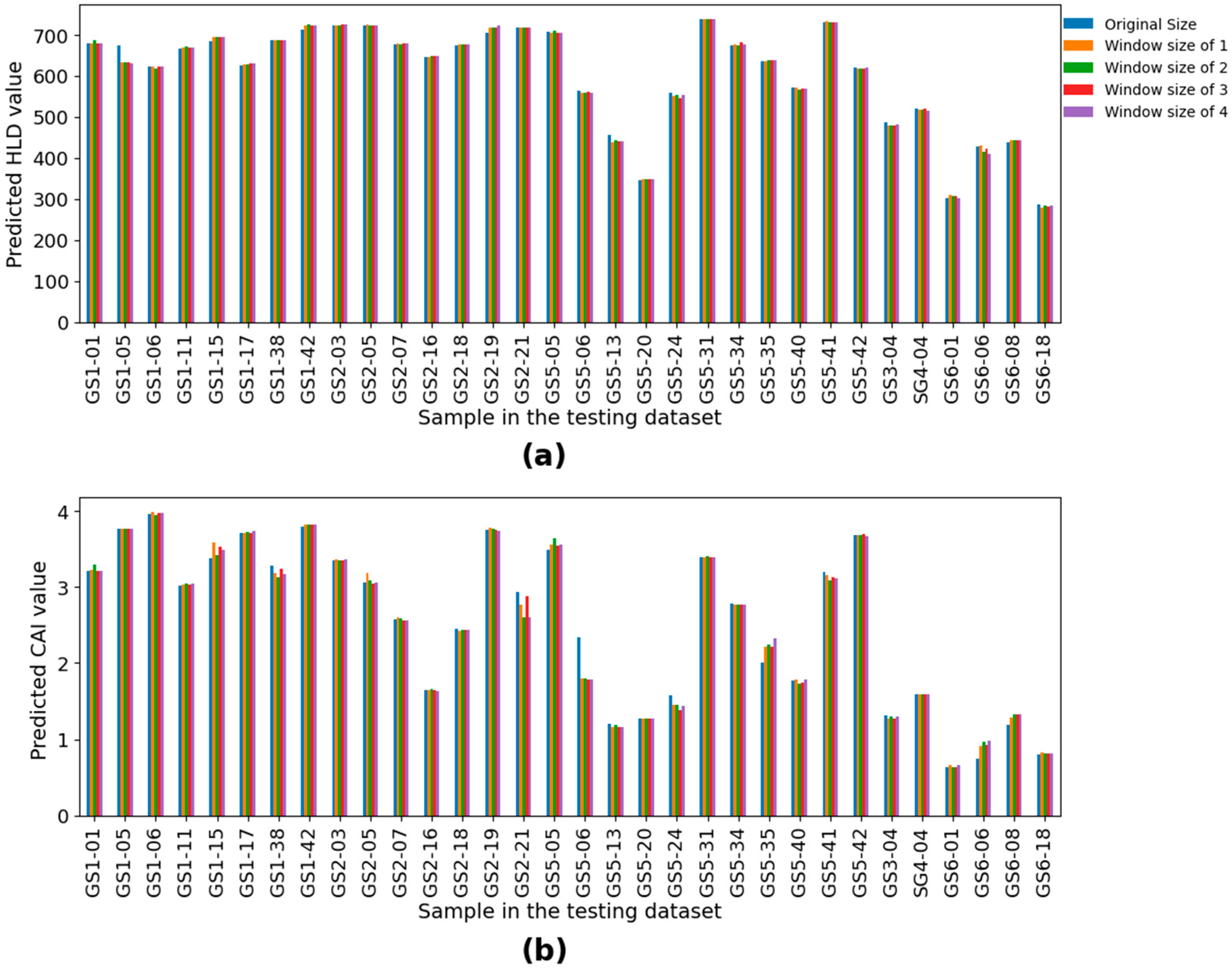
Afterward, the resulting hyperspectral images from the resampling approach were fed into the feature extraction approach, and then the obtained results were fed into the predictive models. Bar plots were used to compare the performance of predicted HLD and CAI values for different window sizes used in the resampling approach (Figure 22). No significant difference between the predicted values using original and resampled images can be observed, which confirms that the proposed model is not considerably affected by the scanning distance.

4. Conclusions

Rock hardness and abrasivity are among the most critical properties of rocks, and they can significantly impact the mine-to-mill process. Accurate and continuous estimation and understanding of the spatial variabilities of rock hardness and abrasivity within the ore deposit can lead to better planning and optimization of the entire mine-to-mill process by allowing informed decisions on equipment selection, process parameters, blending strategies, and maintenance schedules. Currently, there are no remote sensing methods to estimate the rock hardness and abrasivity. Hence, this study utilized the RFR algorithm to predict rock hardness and abrasivity based on hyperspectral imaging as a rapid, nondisruptive, large-scale, and multipurpose data accusation approach. To achieve this, 159 handpicked rock samples were collected from six distinct blasted muck piles within a gold mine, which are mainly sedimentary and ultramafic rocks. The testing procedure consisted of two stages: (1) scanning samples using the hyperspectral VNIR and SWIR sensors, and (2) performing LRH and CAI tests to quantify the hardness and abrasivity of rock samples. Due to the high dimensionality of hyperspectral data, 487 bands, a feature extraction approach based on K-means clustering and band ratio concept was applied to the training dataset, 80% of the samples, resulting in 28 band-ratio-based features.

The preliminary data assessment revealed a significant correlation between HLD and CAI. However, since their relationship was unclear, separate predictive models were developed for HLD and CAI. A Bayesian optimization technique based on the Gaussian process was used to tune the hyperparameters of the RFR algorithm. The performance of the proposed predictive models for HLD and CAI was checked using three statistical indices, including R², RMSE, and VAF, in each case. The obtained results showed that the developed models can effectively predict rock hardness and abrasivity. However, the proposed model for CAI with an R² of 0.79 performed slightly better than the model for HLD with an R² of 0.74. Considering the hyperspectral data as nondestructive remotely sensed data, the obtained results are promising. SHAP analysis was employed to assess the effects of the input features on the performance of predictive models. The obtained results showed that “F_25”, “F_6”, “F_23”, and “F_13” are among the most influential input features for both HLD and CAI models, mainly located within the SWIR region. Therefore, an attempt was made to develop predictive models based solely on SWIR data, which resulted in a 10 percent reduction in R² in both HLD and CAI cases. In the last step, the effects of scanning distance on the performance of proposed models were investigated. The results showed that the proposed feature extraction and predictive models are not affected by increasing the scanning distance up to 9 m. In future works, the effects of other factors, including moisture, dust, illumination, and different scanning distances, will be evaluated in the field.